Approximate Sparse Linear Regression

Abstract

In the Sparse Linear Regression (SLR) problem, given a $d\times n$ matrix ${{M}}$ and a $d$-dimensional query ${{q}}$, the goal is to compute a $k$-sparse $n$-dimensional vector ${{\tau}}$ such that the error $\left\|{{M}}{{\tau}}-{{q}}\right\|$ is minimized. This problem is equivalent to the following geometric problem: given a set $P$ of $n$ points and a query point ${{q}}$ in $d$ dimensions, find the closest $k$-dimensional subspace to ${{q}}$, that is spanned by a subset of $k$ points in $P$. In this paper, we present data-structures/algorithms and conditional lower bounds for several variants of this problem (such as finding the closest induced $k$ dimensional flat/simplex instead of a subspace).

In particular, we present approximation algorithms for the online variants of the above problems with query time $\scalerel*{\widetilde{O}}{j^{2}}(n^{k-1})$, which are of interest in the "low sparsity regime" where $k$ is small, e.g., $2$ or $3$. For $k=d$, this matches, up to polylogarithmic factors, the lower bound that relies on the affinely degenerate conjecture (i.e., deciding if $n$ points in $\mathbb{R}^{d}$ contains $d+1$ points contained in a hyperplane takes $\Omega(n^{d})$ time). Moreover, our algorithms involve formulating and solving several geometric subproblems, which we believe to be of independent interest.

1 Introduction

The goal of the Sparse Linear Regression (SLR) problem is to find a sparse linear model explaining a given set of observations. Formally, we are given a matrix ${{M}}\in\mathbb{R}^{d\times n}$, and a vector ${{q}}\in\mathbb{R}^{d}$, and the goal is to find a vector ${{\tau}}$ that is $k$-sparse (has at most $k$ non-zero entries) and that minimizes $\left\|{{q}}-{{M}}{{\tau}}\right\|_{2}$. The problem also has a natural query/online variant where the matrix ${{M}}$ is given in advance (so that it can be preprocessed) and the goal is to quickly find ${{\tau}}$ given ${{q}}$.

Various variants of SLR have been extensively studied, in a wide range of fields including (i) statistics and machine learning [Tib96, Tib11], (ii) compressed sensing [Don06], and (iii) computer vision [WYG⁺09]. The query/online variant is of particular interest in the application described by Wright et al. [WYG⁺09], where the matrix ${{M}}$ describes a set of image examples with known labels and ${{q}}$ is a new image that the algorithm wants to label.

If the matrix ${{M}}$ is generated at random or satisfies certain assumptions, it is known that a natural convex relaxation of the problem finds the optimum solution in polynomial time [CRT06, CDS98]. However, in general the problem is known to be NP-Hard [Nat95, DMA97], and even hard to approximate up to a polynomial factor [FKT15] (see below for a more detailed discussion). Thus, it is likely that any algorithm for this problem that guarantees "low" approximation factor must run in exponential time. A simple upper bound for the offline problem is obtained by enumerating ${n\choose k}$ possible supports of ${{\tau}}$ and then solving an instance of the $d\times k$ least squares problem. This results in $n^{k}(d+k)^{O(1)}$ running time, which (to the best of our knowledge) constitutes the fastest known algorithm for this problem. At the same time, one can test whether a given set of $n$ points in a $d$-dimensional space is degenerate by reducing it to $n$ instances of SLR with sparsity $d$. The former problem is conjectured to require $\Omega(n^{d})$ time [ES95] – this is the affinely degenerate conjecture. This provides a natural barrier for running time improvements (we elaborate on this below in Section 1.1.1).

In this paper, we study the complexity of the problem in the case where the sparsity parameter $k$ is constant. In addition to the formulation above, we also consider two more constrained variants of the problem. First, we consider the Affine SLR where the vector ${{\tau}}$ is required to satisfy $\left\|{{\tau}}\right\|_{1}=1$, and second, we consider the Convex SLR where additionally ${{\tau}}$ should be non-negative. We focus on the approximate version of these problems, where the algorithm is allowed to output a $k$-sparse vector ${{\tau}}^{\prime}$ such that $\left\|{{M}}{{\tau}}^{\prime}-{{q}}\right\|_{2}$ is within a factor of $1+\varepsilon$ of the optimum.

Geometric interpretation. The SLR problem is equivalent to the Nearest Linear Induced Flat problem defined as follows. Given a set ${{P}}$ of $n$ points in $d$ dimensions and a $d$-dimensional vector ${{q}}$, the task is to find a $k$-dimensional flat spanning a subset $B$ of $k$ points in ${{P}}$ and the origin, such that the (Euclidean) distance from ${{q}}$ to the flat is minimized. The Affine and Convex variants of SLR respectively correspond to finding the Nearest Induced Flat and the Nearest Induced Simplex problems, where the goal is to find the closest $(k-1)$-dimensional flat/simplex spanned by a subset of $k$ points in ${{P}}$ to the query.

Motivation for the problems studied. Given a large set of items (e.g., images), one would like to store them efficiently for various purposes. One option is to pick a relatively smaller subset of representative items (i.e., support vectors), and represent all items as a combination of this supporting set. Note, that if our data-set is diverse and is made out of several distinct groups (say, images of the sky, and images of children), then naturally, the data items would use only some of the supporting set for representation (i.e., the representation over the supporting set is naturally sparse). As such, it is natural to ask for a sparse representation of each item over the (sparse but still relatively large) supporting set. (As a side note, surprisingly little is known about how to choose such a supporting set in theory, and the problem seems to be surprisingly hard even for points in the plane.)

Now, when a new item arrives to the system, the task is to compute its best sparse representation using the supporting set, and we would like to do this as fast as possible (which admittedly is not going to be that fast, see below for details).

Comment Space Query See SLR $\Bigl{.}n^{k-1}{{{S}}}\left({n,\varepsilon}\right)$ $n^{k-1}{{T_{Q}}}\left({n,\varepsilon}\right)$ Theorem 3.7 Affine SLR $\Bigl{.}n^{k-1}{{{S}}}\left({n,\varepsilon}\right)$ $n^{k-1}{{T_{Q}}}\left({n,\varepsilon}\right)$ Theorem 3.6 Convex SLR $\Bigl{.}n^{k-1}{{{S}}}\left({n,\varepsilon}\right)\log^{k}n$ $n^{k-1}{{T_{Q}}}\left({n,\varepsilon}\right)\log^{k}n$ Lemma 4.15 $k=2$ & $\varepsilon\leq 1$ $\Bigl{.}n{{{S}}}\left({n,\varepsilon}\right)\log n$ $n{{T_{Q}}}\left({n,\varepsilon}\right)\varepsilon^{-2}\log n$ Theorem 7.7 Approximate nearest $k=2$ $\bigl{.}2(1+\varepsilon)$ Approx $n^{1+O(\frac{1}{(1+\varepsilon)^{2}})}$ Theorem 5.3 induced segment $d=O(1)$ $\Bigl{.}O(n\log n+n/\varepsilon^{d})$ Corollary 5.4

Table 1.1: Summary of results. Here, ${{{S}}}\left({n,\varepsilon}\right)$ denotes the preprocessing time and space used by a $(1+\varepsilon)$-ANN (approximate nearest-neighbor) data-structure, and ${{T_{Q}}}\left({n,\varepsilon}\right)$ denotes the query time (we assume all these bounds are at least linear in the dimension $d$). All the data-structures, except the last one, provide $(1+\varepsilon)$-approximation. In the nearest induced segment case (i.e., this is the offline convex SLR case) the algorithm answers a single query – in the specific case of Theorem 5.3, the query time is slighly better than the online variant, but significnatly, the space is better by a factor of $n$. Unfortunately, the quality of apprxoimation is worse.

1.1 Our results

Data-structures. We present data-structures to solve the online variants of the SLR, Affine SLR and Convex SLR problems, for general value of $k$. Our algorithms use a provided approximate nearest-neighbor (ANN) data-structure as a black box. The new results are summarized in Table 1.1. For example, for a point set in constant dimension, we get a near linear time algorithm that computes for a single point, the nearest induced segment to it in near linear time, see Corollary 5.4.

For small values of $k$, our algorithms offer notable improvements of the query time over the aforementioned naive algorithm, albeit at a cost of preprocessing. Below in Section 1.1.1, we show how our result matches the lower bound that relies on the affinely degenerate conjecture. Moreover, our algorithms involve formulating and solving several interesting geometric subproblems, which we believe to be of independent interest.

Conditional lower bound. We show a conditional lower bound of $\Omega(n^{k/2}/(e^{k}\log^{\Theta(1)}n))$, for the offline variants of all three problems. Improving this lower bound further, for the case of $k=4$, would imply a nontrivial lower bound for famous Hopcroft’s problem. See Section A for the description. Our lower bound result presented in Section 6, follows by a reduction from the $k$-sum problem which is conjectured to require $\Omega(n^{\lceil k/2\rceil}/\log^{\Theta(1)}n)$ time (see e.g., [PW10], Section 5). This provides further evidence that the off-line variants of the problem require $n^{\Omega(k)}$ time.

1.1.1 Detecting affine degeneracy

Given a point set ${{P}}$ in $\mathbb{R}^{d}$ (here $d$ is conceptually small), it is natural to ask if the points are in general position – that is, all subsets of $d+1$ points are affinely independent. The affinely degenerate conjecture states that this problem requires $\Omega(n^{d})$ time to solve [ES95]. This can be achieved by building the arrangement of hyperplanes in the dual, and detecting any vertex that has $d+1$ hyperplanes passing through it. This problem is also solvable using our data-structure. (We note that since the approximation of our data structure is multiplicative, and in the reduction we only need to detect distance of $0$ from larger than $0$, we are able to solve the exact degeneracy problem as described next). Indeed, we instantiate Theorem 3.6, for $k=d$, and using a low-dimensional $(1+\varepsilon)$-ANN data-structure of Arya et al. [AMN⁺98]. Such an ANN data-structure uses ${{{S}}}\left({n,\varepsilon}\right)=O(n)$ space, $O(n\log n)$ preprocessing time, and ${{T_{Q}}}\left({n,\varepsilon}\right)=O(\log n+1/\varepsilon^{d})=O(\log n)$ query time (for a fixed constant $\varepsilon<1$). Thus, by Theorem 3.6, our data structure has total space usage and preprocessing time of $\tilde{O}(n^{k})$ and a query time of $\tilde{O}(n^{k-1})$. Detecting affine degeneracy then reduces to solving for each point of ${{q}}\in{{P}}$, the problem of finding the closest $(d-1)$-dimensional induced flat (i.e., passing through $d$ points) of ${{P}}\setminus\left\{{{{q}}}\right\}$ to ${{q}}$. It is easy to show that this can be solved using our data-structure with an extra $\log$ factor. This means that the total runtime (including the preprocessing and the $n$ queries) will be $\tilde{O}(n^{k})=\tilde{O}(n^{d})$. Thus, up to polylogarithmic factor, the data-structure of Theorem 3.6 provides an optimal trade-off under the affinely degenerate conjecture. We emphasize that this reduction only rules out the existence of algorithms for online variants of our problems that improve both the preprocessing time from $O(n^{k})$, and query time from $O(n^{k-1})$ by much; it does not rule out for example the algorithms with large preprocessing time (in fact much larger than $n^{k}$) but small query time.

1.2 Related work

The computational complexity of the approximate sparse linear regression problem has been studied, e.g., in [Nat95, DMA97, FKT15]. In particular, the last paper proved a strong hardness result, showing that the problem is hard even if the algorithm is allowed to output a solution with sparsity $k^{\prime}=k2^{\log^{1-\delta}n}$ whose error is within a factor of $n^{c}m^{1-\alpha}$ from the optimum, for any constants $\delta,\alpha>0$ and $c>1$.

The query/online version of the Affine SLR problem can be reduced to the Nearest $k$-flat Search Problem studied in [Mag02, BHZM11, Mah15], where the database consists of a set of $k$-flats (affine subspaces) of size $N$ and the goal is to find the closest $k$-flat to a given query point ${{q}}$. Let ${{P}}$ be a set of $n$ points in $\mathbb{R}^{d}$ that correspond to the columns of ${{M}}$. The reduction proceeds by creating a database of all $N=\binom{n}{k}$ possible $k$-flats that pass through $k$ points of ${{P}}$. However, the result of [BHZM11] does not provide multiplicative approximation guarantees, although it does provide some alternative guarantees and has been validated by several experiments. The result of [Mag02], provides provable guarantees and fast query time of $(d+\log N+1/\varepsilon)^{O(1)}$, but the space requirement is quasi-polynomial of the form $2^{(\log N)^{O(1)}}=2^{(k\log n)^{O(1)}}$. Finally the result of [Mah15] only works for the special case of $k=2$, and yields an algorithm with space usage $O\left({n^{14}\varepsilon^{-3}{{{S}}}\left({n^{2},\varepsilon}\right)}\right)$ and query time $O\left({{{T_{Q}}}\left({{n^{2}\varepsilon^{-4}},\varepsilon}\right)\log^{2}n}\right)$. Similar results can be achieved for the other variants.

The SLR problem has a close relationship with the Approximate Nearest Neighbor (ANN) problem. In this problem, we are given a collection of $N$ points, and the goal is to build a data structure which, given any query point ${{q}}$, reports the data point whose distance to the query is within a $(1+\varepsilon)$ factor of the distance of the closest point to the query. There are many efficient algorithms known for the latter problem. One of the state of the art results for ANN in Euclidean space answers queries in time $(d\log(N)/\varepsilon^{2})^{O(1)}$ using $(dN)^{O(1/\varepsilon^{2})}$ space [KOR00, IM98].

1.3 Our techniques and sketch of the algorithms

Affine SLR (nearest flat). To solve this problem, we first fix a subset ${{B}}\subseteq P$ of $k-1$ points, and search for the closest $(k-1)$-flat among those that contain ${{B}}$. Note, that there are at most $n-k+1$ such flats. Each such flat ${{\mathsf{f}}}$, as well as the query flat $Q_{\mathrm{flat}}$ (containing ${{B}}$ and the query ${{q}}$), has only one additional degree of freedom, which is represented by a vector $v_{H}$ ($v_{Q}$, resp.) in a $d-k+1$ space. The vector $v_{H}$ that is closest to $v_{Q}$ corresponds to the flat that is closest to ${{q}}$. This can be found approximately using standard ANN data structure, resulting in an algorithm with running time $O(n^{k-1}\cdot{{T_{Q}}}\left({n,\varepsilon}\right))$. Similarly, by adding the origin to the set ${{B}}$, we could solve the SLR problem in a similar way.

Convex SLR (nearest simplex). This case requires an intricate combination of low and high dimensional data structures, and is the most challenging part of this work. To find the closest $(k-1)$-dimensional induced simplex, one approach would be to fix ${{B}}$ as before, and find the closest corresponding flat. This will work only if the projection of the query onto the closest flat falls inside of its corresponding simplex. Because of that, we need to restrict our search to the flats of feasible simplices, i.e., the simplices $S$ such that the projection of the query point onto the corresponding flat falls inside $S$. If we manage to find this set, we can use the algorithm for affine SLR to find the closest one. Note that finding the distance of the query to the closest non-feasible simplex can easily be computed in time $n^{k-1}$ as the closest point of such a simplex to the query lies on its boundary which is a lower dimensional object.

Let $S$ be the unique simplex obtained from ${{B}}$ and an additional point ${{p}}$. Then we can determine whether $S$ is feasible or not only by looking at (i) the relative positioning of ${{p}}$ with respect to ${{B}}$, that is, how the simplex looks like in the flat going through $S$, (ii) the relative positioning of ${{q}}$ with respect to ${{B}}$, and (iii) the distance between the query and the flat of the simplex. Thus, if we were given a set of simplices through ${{B}}$ such that all their flats were at a distance $r$ from the query, we could build a single data structure for retrieving all the feasible flats. This can be done by mapping all of them in advance onto a unified $(k-1)$ dimensional space (the “parameterized space”), and then using $k-1$ dimensional orthogonal range-searching trees in that space.

However, the minimum distance $r$ is not known in general. Fortunately, as we show the feasibility property is monotone in the distance: the farther the flat of the simplex is from the query point, the weaker constraints it needs to satisfy. Thus, given a threshold value $r$, our algorithm retrieves the simplices satisfying the restrictions they need to satisfy if they were at a distance $r$ from the query. This allows us to use binary search for finding the right value of $r$ by random sampling. The final challenge is that, since our access is to an approximate NN data structure (and not an exact one), the above procedure yields a superset of feasible simplices. The algorithm then finds the closest flat corresponding to the simplices in this superset. We show that although the reported simplex may not be feasible (the projection of ${{q}}$ on to the corresponding flat does not fall inside the simplex), its distance to the query is still approximately at most $r$.

Convex SLR for $k=2$ (offline nearest segment). Given a set of $n$ points ${{P}}$ and the query ${{q}}$ all at once, the goal is to find the segment composed of two points in ${{P}}$ that is closest to the query, in sub-quadratic time. To this end, we project the point set to a sphere around the query point, and preprocess it for ANN. For each point of ${{P}}$, we use its reflected point on the sphere, to perform an ANN query, and get another (projected) point. Taking the original two points, generates a segment. We prove that among these $n$ segments, there is a $O(1)$-ANN to the closest induced segment. This requires building ANN data-structure and answering $n$ ANN queries, thus yielding a subquadratic-time algorithm. See Section 5 for details.

Conditional Lower bound. Our reduction from $k$-sum is randomized, and based on the following idea. First observe that by testing whether the solution to SLR is zero or non-zero we can test whether there is a subset of $k$ numbers and a set of associated $k$ weights such that the weighted sum is equal to zero. In order to solve $k$-sum, however, we need to force the weights to be equal to $1$. To this end, we lift the numbers to vectors, by extending each number by a vector selected at random from the standard basis $e_{1}\ldots e_{k}$. We then ensure that in the selected set of $k$ numbers, each element from the basis is represented exactly once and with weight 1. This ensures that the solution to SLR yields a feasible solution to $k$-sum.

2 Preliminaries

2.1 Notations

Throughout the paper, we assume ${{P}}\subseteq\mathbb{R}^{d}$ is the set of input points which is of size $n$. In this paper, for simplicity, we assume that the point-sets are non-degenerate, however this assumption is not necessary for the algorithms. We use the notation $X\subset_{i}B$ to denote that $X$ is a subset of $B$ of size $i$, and use 0 to denote the origin. For two points ${{y}},{{u}}\in\mathbb{R}^{d}$, the segment the form is denoted by ${{y}}{{u}}$, and the line formed by them by $\mathrm{line}\left({{{y}},{{u}}}\right)$.

Definition 2.1.

For a set of points $S$, let ${{\mathsf{f}}}_{S}=\mathrm{aff}\left({S}\right)=\left\{\sum_{i=1}^{\left|{S}\right|}\alpha_{i}{{p}}_{i}\;\middle|\;{{p}}_{i}\in S,\text{ and }\sum_{i=1}^{\left|{S}\right|}\alpha_{i}=1\right\}$ be the $(\left|{S}\right|-1)$-dimensional flat (or $(\left|{S}\right|-1)$-flat for short) passing through the points in the set $S$ (aka the affine hull of $S$). The $(\left|{S}\right|-1)$-dimensional simplex ($({\left|{S}\right|}-1)$-simplex for short) that is formed by the convex-hull of the points of $S$ is denoted by ${{{{\triangle}}}}_{S}$. We denote the interior of a simplex ${{{{\triangle}}}}_{S}$ by $\mathrm{int}\left({{{{{\triangle}}}}_{S}}\right)$.

Definition 2.2 (distance and nearest-neighbor).

For a point ${{q}}\in\mathbb{R}^{d}$, and a point ${{p}}\in\mathbb{R}^{d}$, we use ${{\mathsf{d}}}({{q}},{{p}})=\left\|{{q}}-{{p}}\right\|_{2}$ to denote the distance between ${{q}}$ and ${{p}}$. For a closed set ${{X}}\subseteq\mathbb{R}^{d}$, we denote by ${{\mathsf{d}}}({{q}},{{X}})=\min_{{{p}}\in{{X}}}\left\|{{q}}-{{p}}\right\|_{2}$ the distance between ${{q}}$ and ${{X}}$. The point of ${{X}}$ realizing the distance between ${{q}}$ and ${{X}}$ is the nearest neighbor to ${{q}}$ in ${{X}}$, denoted by $\mathsf{nn}\left({{{q}},{{X}}}\right)$. We sometimes refer to $\mathsf{nn}\left({{{q}},{{X}}}\right)$ as the projection of ${{q}}$ onto ${{X}}$.

More generally, given a finite family of such sets ${{\mathcal{G}}}=\left\{{{X}}_{i}\subseteq\mathbb{R}^{d}\;\middle|\;i=1,\ldots,m\right\}$, the distance of ${{q}}$ from ${{\mathcal{G}}}$ is ${{\mathsf{d}}}({{q}},{{\mathcal{G}}})=\min_{{{X}}\in{{\mathcal{G}}}}{{\mathsf{d}}}({{q}},{{X}})$. The nearest-neighbor $\mathsf{nn}\left({{{q}},{{\mathcal{G}}}}\right)$ is defined analogously to the above.

Assumption 2.3.

Throughout the paper, we assume we have access to a data structure that can answer $(1+\varepsilon)$-ANN queries on a set of $n$ points in $\mathbb{R}^{d}$. We use ${{{S}}}\left({n,\varepsilon}\right)$ to denote the space requirement of this data structure, and by ${{T_{Q}}}\left({n,\varepsilon}\right)$ to denote the query time.

2.1.1 Induced stars, bouquets, books, simplices and flats

Definition 2.4.

Given a point ${{b}}$ and a set ${{P}}$ of points in $\mathbb{R}^{d}$, the star of ${{P}}$, with the base ${{b}}$, is the set of segments ${{\mathrm{star}}}\left({{{b}},{{P}}}\right)=\left\{{{b}}{{p}}\;\middle|\;{{p}}\in{{P}}\setminus\left\{{{{b}}}\right\}\right\}.$ Similarly, given a set ${{B}}$ of points in $\mathbb{R}^{d}$, with $\left|{{{B}}}\right|=k-1\leq d$, the book of ${{P}}$, with the base ${{B}}$, is the set of simplices ${{\bm{\Delta}}}\left({{{B}},{{P}}}\right)=\left\{{{{{\triangle}}}}_{{{B}}\cup\left\{{{{p}}}\right\}}\;\middle|\;{{p}}\in{{P}}\setminus{{B}}\right\}.$ Finally, the set of flats induced by these simplices, is the bouquet of ${{P}}$, denoted by ${{\mathrm{bqt}}}\left({{{B}},{{P}}}\right)=\left\{{{\mathsf{f}}}_{{{B}}\cup\left\{{{{p}}}\right\}}\;\middle|\;{{p}}\in{{P}}\setminus{{B}}\right\}.$

If ${{B}}$ is a single point, then the corresponding book is a star, and the corresponding bouquet is a set of lines all passing through the single point in ${{B}}$.

Definition 2.5.

For a set ${{P}}\subseteq\mathbb{R}^{d}$, let ${{\mathcal{L}_{k}\left({{{P}}}\right)}}=\left\{{{\mathsf{f}}}_{S\cup\{{{\textbf{0}}}\}}\;\middle|\;S\subset_{k}{{P}}\right\}$ be the set of all linear $k$-dimensional subspaces induced by ${{{P}}}$, and ${{\mathcal{F}_{k}\left({{{P}}}\right)}}=\left\{{{\mathsf{f}}}_{S}\;\middle|\;S\subset_{k}{{P}}\right\}$ be the set of all $(k-1)$-flats induced by ${{P}}$. Similarly, let ${{\bm{\Delta}_{k}\left({{{P}}}\right)}}=\left\{{{{{\triangle}}}}_{S}\;\middle|\;S\subset_{k}{{P}}\right\}$ be the set of all $(k-1)$-simplices induced by ${{P}}$.

2.2 Problems

In the following, we are given a set ${{P}}$ of $n$ points in $\mathbb{R}^{d}$, a query point ${{q}}$ and parameters $k$ and $\varepsilon>0$. We are interested in the following problems:

1. SLR (nearest induced linear subspace): Compute $\mathsf{nn}\left({{{q}},\bigl{.}{{\mathcal{L}_{k}\left({{{P}}}\right)}}}\right)$.

2. ANLIF (approximate nearest linear induced flat): Compute a $k$-flat ${{\mathsf{f}}}\in{{\mathcal{L}_{k}\left({{{P}}}\right)}}$, such that ${{\mathsf{d}}}({{q}},{{\mathsf{f}}})\leq(1+\varepsilon){{\mathsf{d}}}({{q}},\bigl{.}{{\mathcal{L}_{k}\left({{{P}}}\right)}})$.

3. Affine SLR (nearest induced flat): Compute $\mathsf{nn}\left({{{q}},\bigl{.}{{\mathcal{F}_{k}\left({{{P}}}\right)}}}\right)$.

4. ANIF (Approximate Nearest Induced Flat): Compute a $(k-1)$-flat ${{\mathsf{f}}}\in{{\mathcal{F}_{k}\left({{{P}}}\right)}}$, such that ${{\mathsf{d}}}({{q}},{{\mathsf{f}}})\leq(1+\varepsilon){{\mathsf{d}}}({{q}},\bigl{.}{{\mathcal{F}_{k}\left({{{P}}}\right)}})$.

5. Convex SLR (Nearest Induced Simplex): Compute $\mathsf{nn}\left({{{q}},\bigl{.}{{\bm{\Delta}_{k}\left({{{P}}}\right)}}}\right)$.

6. ANIS (Approximate Nearest Induced Simplex): Compute a $(k-1)$-simplex ${{\triangle}}\in{{\bm{\Delta}_{k}\left({{{P}}}\right)}}$, such that ${{\mathsf{d}}}({{q}},{{\triangle}})\leq(1+\varepsilon){{\mathsf{d}}}({{q}},\bigl{.}{{\bm{\Delta}_{k}\left({{{P}}}\right)}})$.

Here, the parameter $k$ corresponds to the sparsity of the solution.

3 Approximating the nearest induced flats and subspaces

In this section, we show how to solve approximately the online variants of SLR and affine SLR problems. These results are later used in Section 4. We start with the simplified case of the uniform star.

3.1 Approximating the nearest neighbor in a uniform star

Input & task. We are given a base point ${{b}}$, a set ${{P}}$ of $n$ points in $\mathbb{R}^{d}$, and a parameter $\varepsilon>0$. We assume that $\left\|{{b}}-{{p}}\right\|=1$, for all ${{p}}\in{{P}}$. The task is to build a data structure that can report quickly, for a query point ${{q}}$ that is also at distance one from ${{b}}$, the $(1+\varepsilon)$-ANN segment to ${{q}}$ in ${{\mathrm{star}}}\left({{{b}},{{P}}}\right)$.

Preprocessing. The algorithm computes the set ${{V}}=\left\{{{p}}-{{b}}\;\middle|\;{{p}}\in{{P}}\setminus\left\{{{{b}}}\right\}\right\}$, which lies on a unit sphere in $\mathbb{R}^{d}$. Next, the algorithm builds a data structure ${{\mathcal{D}}}_{{V}}$ for answering $(1+\varepsilon)$-ANN queries on ${{V}}$.

Answering a query. For a query point ${{q}}$, the algorithm does the following:

1. Compute ${{\tau}}={{q}}-{{b}}$.

2. Compute $(1+\varepsilon)$-ANN to ${{\tau}}$ in ${{V}}$, denoted by ${{u}}$ using ${{\mathcal{D}}}_{{V}}$.

3. Let ${{y}}$ be the point in ${{P}}$ corresponding to ${{u}}$.

4. Return $\min\left({\bigl{.}{{\mathsf{d}}}({{q}},{{b}}{{y}}),\,1}\right)$.

Lemma 3.1.

Consider a base point ${{b}}$, and a set ${{P}}$ of $n$ points in $\mathbb{R}^{d}$ all on ${{\mathbb{S}}}\left({{{b}},1}\right)$, where ${{\mathbb{S}}}={{\mathbb{S}}}\left({{{b}},1}\right)$ is the sphere of radius $1$ centered at ${{b}}$. Given a query point ${{q}}\in{{\mathbb{S}}}$, the above algorithm reports correctly a $(1+\varepsilon)$-ANN in ${{\mathrm{star}}}\left({{{b}},{{P}}}\right)$. The query time is dominated by the time to perform a single $(1+\varepsilon)$-ANN query.

Proof:

If ${{\mathsf{d}}}({{q}},{{\mathrm{star}}}\left({{{b}},{{P}}}\right))=1$ the correctness is obvious. Otherwise, ${{\mathsf{d}}}({{q}},{{\mathrm{star}}}\left({{{b}},{{P}}}\right))<1$, and assume for the sake of simplicity of exposition that ${{b}}$ is the origin. Let ${{x}}$ be the nearest neighbor to ${{q}}$ in ${{P}}$, and let ${{x}}^{\prime}$ be the nearest point on ${{b}}{{x}}$ to ${{q}}$. Similarly, let ${{y}}$ be the point returned by the ANN data structure for ${{q}}$, and let ${{y}}^{\prime}$ be the nearest point on ${{b}}{{y}}$ to ${{q}}$. Moreover, let $\alpha=\measuredangle{{q}}{{b}}{{x}}$ and $\beta=\measuredangle{{q}}{{b}}{{y}}$. As ${{\mathsf{d}}}({{q}},{{\mathrm{star}}}\left({{{b}},{{P}}}\right))<1$, we can also conclude that $\alpha$ is smaller than $\pi/2$.

We have that $\left\|{{q}}-{{x}}\right\|\leq\left\|{{q}}-{{y}}\right\|\leq(1+\varepsilon)\left\|{{q}}-{{x}}\right\|.$ Observe that $\left\|{{q}}-{{y}}\right\|=2\sin(\beta/2),$ and $\left\|{{q}}-{{x}}\right\|=2\sin(\alpha/2).$ As such, by the monotonicity of the $\sin$ function in the range $[0,\pi/2]$, we conclude that $\alpha\leq\beta$. This readily implies that ${{x}}$ is the point of ${{P}}$ that minimizes the angle $\measuredangle{{q}}{{b}}{{x}}$ (i.e., $\alpha$), which in turn minimizes the distance to ${{q}}$ on the induced segment. As such, we have ${{\mathsf{d}}}({{q}},{{\mathrm{star}}}\left({{{b}},{{P}}}\right))=\left\|{{q}}-{{x}}^{\prime}\right\|.$

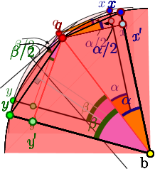
Figure 3.1:

As for the quality of approximation, first suppose that $\beta\leq\pi/2$. Then we have $\frac{\left\|{{q}}-{{y}}^{\prime}\right\|}{\left\|{{q}}-{{x}}^{\prime}\right\|}=\frac{\left\|{{q}}-{{y}}\right\|\cos(\beta/2)}{\left\|{{q}}-{{x}}\right\|\cos(\alpha/2)}\leq 1+\varepsilon,$ since $\left\|{{q}}-{{y}}\right\|/\left\|{{q}}-{{x}}\right\|\leq 1+\varepsilon$ and $\alpha/2\leq\beta/2\leq\pi/2$, which in turn implies that $\cos(\beta/2)\leq\cos(\alpha/2)$.

Otherwise, we know that $\beta>\pi/2$ and thus ${{\mathsf{d}}}({{q}},{{b}}{{y}})=1$. Now if $1\leq(1+\varepsilon)\left\|{{q}}-{{x}}^{\prime}\right\|$ we are done. Thus, we assume that $\left\|{{q}}-{{x}}^{\prime}\right\|\leq 1/(1+\varepsilon)$. Also, we have that $\left\|{{q}}-{{x}}\right\|\geq\left\|{{q}}-{{y}}\right\|/(1+\varepsilon)>\sqrt{2}/(1+\varepsilon)$ as $\beta>\pi/2$. This would imply that $\sqrt{2}/(1+\varepsilon)<\left\|{{q}}-{{x}}\right\|=\left\|{{q}}-{{x}}^{\prime}\right\|/\cos(\alpha/2)\leq 2/\sqrt{2}(1+\varepsilon)$, as $\alpha\leq\pi/2$, which is a contradiction. Hence, the lemma holds.  

3.2 Approximating the nearest flat in a bouquet

Definition 3.2.

For a set ${{X}}$ and a point ${{p}}$ in $\mathbb{R}^{d}$, let ${{p}}^{\prime}=\mathsf{nn}\left({{{p}},{{X}}}\right)$. We use $\mathsf{dir}({{X}},{{p}})$ to denote the unit vector $({{p}}-{{p}}^{\prime})/\left\|{{p}}-{{p}}^{\prime}\right\|$, which is the direction of ${{p}}$ in relation to ${{X}}$.

Input & task. We are given sets ${{B}}$ and ${{P}}$ of $k-1$ and $n$ points, respectively, in $\mathbb{R}^{d}$, and a parameter $\varepsilon>0$. The task is to build a data structure that can report quickly, for a query point ${{q}}$, a $(1+\varepsilon)$-ANN flat to ${{q}}$ in ${{\mathrm{bqt}}}\left({{{B}},{{P}}}\right)$, see Definition 2.4.

Preprocessing. Let ${{F}}={{\mathsf{f}}}_{{{B}}}$. The algorithm computes the set ${{V}}=\left\{\mathsf{dir}({{F}},{{p}}),-\mathsf{dir}({{F}},{{p}})\;\middle|\;{{p}}\in{{P}}\setminus{{B}}\right\},$ which lies on a $d-k+2$ dimensional unit sphere in $\mathbb{R}^{d-k+1}$, and then builds a data structure ${{\mathcal{D}}}_{{V}}$ for answering (standard) ANN queries on ${{V}}$.

Answering a query. For a query point ${{q}}$, the algorithm does the following:

1. Compute ${{\tau}}=\mathsf{dir}({{F}},{{q}})$.

2. Compute ANN to ${{\tau}}$ in ${{V}}$, denoted by ${{u}}$ using the data structure ${{\mathcal{D}}}_{{V}}$.

3. Let ${{p}}$ be the point in ${{P}}$ corresponding to ${{u}}$.

4. Return the distance ${{\mathsf{d}}}({{q}},{{\mathsf{f}}}_{{{B}}\cup\left\{{{{p}}}\right\}})$.

Definition 3.3.

For sets ${{X}},{{Y}}\subseteq\mathbb{R}^{d}$, let ${{\mathsf{proj}}}_{{{X}}}\left({{{Y}}}\right)=\left\{\mathsf{nn}\left({{{q}},{{X}}}\right)\;\middle|\;{{q}}\in{{Y}}\right\}$ be the projection of ${{Y}}$ on ${{X}}$.

Lemma 3.4.

Consider two affine subspaces ${{F}}\subseteq{{H}}$ with a base point ${{b}}\in{{F}}$, and the orthogonal complement affine subspace ${{{F}}}^{\bot}=\left\{{{b}}+{{\tau}}\;\middle|\;\bigl{.}\left\langle{{{{\tau}}},{{{u}}-{{v}}}}\right\rangle=0\text{ for all }{{u}},{{v}}\in{{F}},{{\tau}}\in\mathbb{R}^{d}\right\}\!.$ For an arbitrary point ${{q}}\in\mathbb{R}^{d}$, let ${{{q}}}^{\bot}={{\mathsf{proj}}}_{{{{F}}}^{\bot}}\left({{{q}}}\right)$.We have that ${{\mathsf{d}}}({{q}},{{H}})={{\mathsf{d}}}({{{q}}}^{\bot},{{\mathsf{proj}}}_{{{{F}}}^{\bot}}\left({{{H}}}\right)).$

Proof:

For the sake of simplicity of exposition, assume that ${{b}}$ is the origin. Let ${{G}}={{{F}}}^{\bot}\cap{{H}}$. We have that ${{F}}$ and ${{G}}$ are both contained in ${{H}}$, and are orthogonal to each other. Furthermore, we have ${{H}}={{F}}+{{G}}$. Setting $f=\mathrm{dim}\left({{{F}}}\right)$, $g=\mathrm{dim}\left({{{G}}}\right)$, and $h=\mathrm{dim}\left({{{H}}}\right)$, we have $h=f+g$, and ${{\mathsf{proj}}}_{{{{F}}}^{\bot}}\left({{{H}}}\right)={{\mathsf{proj}}}_{{{{F}}}^{\bot}}\left({{{F}}+{{G}}}\right)={{\mathsf{proj}}}_{{{{F}}}^{\bot}}\left({{{F}}}\right)+{{\mathsf{proj}}}_{{{{F}}}^{\bot}}\left({{{G}}}\right)={{G}}.$

So, assume that the ${{F}}$ spans the first $f$ coordinates of $\mathbb{R}^{d}$, and ${{G}}$ spans the next $g$ coordinates (i.e., ${{H}}$ is the linear subspace defined by the first $h$ coordinates). If ${{q}}=(q_{1},\ldots,q_{d})$, then ${{{q}}}^{\bot}=(0,\ldots,0,q_{f+1},\ldots,q_{d})$, and

$${{\mathsf{d}}}({{q}},{{H}})=\sqrt{\sum_{i=h+1}^{d}q_{i}^{2}}=\sqrt{\sum_{i=1}^{f}0^{2}+\sum_{i=h+1}^{d}q_{i}^{2}}={{\mathsf{d}}}({{{q}}}^{\bot},{{G}})={{\mathsf{d}}}({{{q}}}^{\bot},{{\mathsf{proj}}}_{{{{F}}}^{\bot}}\left({{{G}}}\right)).$$

 

Using the notation of Assumption 2.3 and Definition 2.4, we have the following:

Lemma 3.5 (ANN flat in a bouquet).

Given sets ${{B}}$ and ${{P}}$ of $k-1$ and $n$ points, respectively, in $\mathbb{R}^{d}$, and a parameter $\varepsilon>0$, one can preprocess them, using a single ANN data structure, such that given a query point, the algorithm can compute a $(1+\varepsilon)$-ANN to the closest $(k-1)$-flat in ${{\mathrm{bqt}}}\left({{{B}},{{P}}}\right)$. The algorithm space and preprocessing time is $O({{{S}}}\left({n,\varepsilon}\right))$, and the query time is $O({{T_{Q}}}\left({n,\varepsilon}\right))$.

Proof:

The construction is described above, and the space and query time bounds follow directly from the algorithm description. As for correctness, pick an arbitrary base point ${{b}}\in{{B}}$, and let ${{{F}}}^{\bot}$ be the orthogonal complement affine subspace to ${{F}}$ passing through ${{b}}$. Let ${{{P}}}^{\bot}={{\mathsf{proj}}}_{{{{F}}}^{\bot}}\left({{{P}}}\right)$, and observe that ${{\mathsf{proj}}}_{{{{F}}}^{\bot}}\left({{{B}}}\right)$ is the point ${{b}}$. In particular, the projection of ${{\mathcal{B}}}={{\mathrm{bqt}}}\left({{{B}},{{P}}}\right)$ to ${{{F}}}^{\bot}$ is the bouquet of lines ${{{\mathcal{B}}}}^{\bot}={{\mathrm{bqt}}}\left({\left\{{{{b}}}\right\},{{{P}}}^{\bot}}\right)$. Applying Lemma 3.4 to each flat of ${{\mathcal{B}}}$, implies that ${{\mathsf{d}}}({{q}},{{\mathcal{B}}})={{\mathsf{d}}}({{{q}}}^{\bot},{{{\mathcal{B}}}}^{\bot})$, where ${{{q}}}^{\bot}={{\mathsf{proj}}}_{{{{F}}}^{\bot}}\left({{{q}}}\right)$. Let ${{\mathbb{S}}}$ be the sphere of radius $r=\left\|{{{q}}}^{\bot}-{{b}}\right\|$ centered at ${{b}}$. Clearly, the closest line in the bouquet, is the closest point to the uniform star formed by clipping the lines of ${{{\mathcal{B}}}}^{\bot}$ to ${{\mathbb{S}}}$. Since all the lines of ${{{\mathcal{B}}}}^{\bot}$ pass through ${{b}}$, scaling space around ${{b}}$ by some factor $\alpha$, just scales the distances between ${{q}}$ and ${{{\mathcal{B}}}}^{\bot}$ by $x$. As such, scale space so that $r=1$. But then, this is a uniform star with radius $1$, and the algorithm of Lemma 3.1 applies (which is exactly what the current algorithm is doing). Thus, it correctly identifies a line in the bouquet that realizes the desired approximation, implying the correctness of the query algorithm.  

3.3 The result

Here, we show simple algorithms for the ANIF and the ANLIF problems by employing Lemma 3.5. We assume $\varepsilon>0$ is a prespecified approximation parameter.

Approximating the affine SLR. As discussed earlier, the goal is to find an approximately closest $(k-1)$-dimensional flat that passes through $k$ points of ${{P}}$, to the query. To this end, we enumerate all possible $k-1$ subsets of points of ${{B}}\subset_{k-1}{{P}}$, and build for each such base set ${{B}}$, the data structure of Lemma 3.5. Given a query, we compute the ANN flat in each one of these data structures, and return the closest one found.

Theorem 3.6.

The aforementioned algorithm computes a $(1+\varepsilon)$-ANN to the closest $(k-1)$-flat in ${{\mathcal{F}_{k}\left({{{P}}}\right)}}$, see Definition 2.5. The space and preprocessing time is $O(n^{k-1}{{{S}}}\left({n,\varepsilon}\right))$, and the query time is $O(n^{k-1}{{T_{Q}}}\left({n,\varepsilon}\right))$.

Approximating the SLR. The goal here is to find an approximately closest $k$-dimensional flat that passes through $k$ points of ${{P}}$ and the origin 0, to the query. We enumerate all possible $k-1$ subsets of points of ${{B}}^{\prime}\subset_{k-1}{{P}}$, and build for each base set ${{B}}={{B}}^{\prime}\cup\{{{\textbf{0}}}\}$, the data structure of Lemma 3.5. Given a query, we compute the ANN flat in each one of these data structures, and return the closest one found.

Theorem 3.7.

The aforementioned algorithm computes a $(1+\varepsilon)$-ANN to the closest $k$-flat in ${{\mathcal{L}_{k}\left({{{P}}}\right)}}$, see Definition 2.5, with space and preprocessing time of $O(n^{k-1}{{{S}}}\left({n,\varepsilon}\right))$, and the query time of $O(n^{k-1}\allowbreak{{T_{Q}}}\left({n,\varepsilon}\right))$.

4 Approximating the nearest induced simplex

In this section we consider the online variant of the ANIS problem. Here, we are given the parameter $k$, and the goal is to build a data structure, such that given a query point ${{q}}$, it can find a $(1+\varepsilon)$-ANN induced $(k-1)$-simplex.

As before, we would like to fix a set ${{B}}$ of $k-1$ points and look for the closest simplex that contains ${{B}}$ and an additional point from ${{P}}$. The plan is to filter out the simplices for which the projection of the query on to them falls outside of the interior of the simplex. Then we can use the algorithm of the previous section to find the closest flat corresponding to the feasible simplices (the ones that are not filtered out). First we define a canonical space and map all these simplices and the query point to a unique $(k+1)$-dimensional space. As it will become clear shortly, the goal of this conversion is to have a common lower dimensional space through which we can find all feasible simplices using range searching queries.

4.1 Simplices and distances

4.1.1 Canonical realization

In the following, we fix a sequence ${{B}}=\left({{{p}}_{1},\ldots,{{p}}_{k-1}}\right)$ of $k-1$ points in $\mathbb{R}^{d}$. We are interested in arguing about simplices induced by $k+1$ points, i.e., ${{B}}$, an additional input point ${{p}}_{k}$, and a query point ${{q}}$. Since the ambient dimension is much higher (i.e., $d$), it would be useful to have a common canonical space, where we can argue about all entities.

Definition 4.1.

For a given set of points ${{B}}$, let ${{F}}={{\mathsf{f}}}_{{{B}}}$. Let ${{p}}\notin{{F}}$ be a given point in $\mathbb{R}^{d}$, and consider the two connected components of ${{\mathsf{f}}}_{{{B}}\cup\{{{p}}\}}\setminus{{F}}$, which are halfflats. The halfflat containing ${{p}}$ is the positive halfflat, and it is denoted by ${{\mathsf{f}}}^{+}\left({{{B}},{{p}}}\right)$.

Fix some arbitrary point ${{\bm{s}}}^{*}\in\mathbb{R}^{d}\setminus{{F}}$, and let ${{G}}={{\mathsf{f}}}^{+}\left({{{B}},{{\bm{s}}}^{*}}\right)$ be a canonical such halfflat. Similarly, for a fixed point ${{\bm{s}}}^{**}\in\mathbb{R}^{d}\setminus{{\mathsf{f}}}_{{{B}}\cup\left\{{{{\bm{s}}}^{*}}\right\}}$, let ${{H}}={{\mathsf{f}}}^{+}\left({{{B}}\cup{{\bm{s}}}^{*},{{\bm{s}}}^{**}}\right)$. Conceptually, it is convenient to consider ${{H}}=\mathbb{R}^{k-2}\times\mathbb{R}\times\mathbb{R}^{+}$, where the first $k-2$ coordinates correspond to ${{F}}$, and the first $k-1$ coordinates correspond to ${{G}}$ (this can be done by applying a translation and a rotation that maps ${{H}}$ into this desired coordinates system). This is the canonical parameterization of ${{H}}$.

The following observation formalizes the following: Given a $(k-1)$ dimensional halfflat ${{G}}$ passing through ${{B}}$, a point on ${{G}}$ is uniquely identified by its distances from the points in ${{B}}$.

Observation 4.2.

Given a sequence of distances $\bm{{{\bm{\ell}}}}=\left({{{\ell}}_{1},\ldots,{{\ell}}_{k-1}}\right)$, there might be only one unique point ${{p}}={{p}}_{{{G}}}\left({{{\bm{\ell}}}}\right)\in{{G}}$, such that $\left\|{{p}}-{{p}}_{i}\right\|={{\ell}}_{i}$, for $i=1,\ldots,k-1$. Such a point might not exist at all.

Next, given ${{G}}$ and ${{H}}$, a point ${{q}}$ and a value ${{\ell}}<{{\mathsf{d}}}({{q}},{{F}})$, we aim to define the points ${{q}}_{{{G}}}\left({{{\ell}}}\right)$ and ${{q}}_{{{H}}}\left({{{\ell}}}\right)$. Consider a point ${{q}}\in\mathbb{R}^{d}\setminus{{F}}$ (not necessarily the query point), and consider any positive $(k-1)$-halfflat ${{\mathsf{g}}}$ that contains ${{B}}$, and is in distance ${{\ell}}$ from ${{q}}$. Furthermore assume that ${{\ell}}={{\mathsf{d}}}({{q}},{{\mathsf{g}}})<{{\mathsf{d}}}({{q}},{{F}}).$ Let ${{q}}_{{{\mathsf{g}}}}$ be the projection of ${{q}}$ to ${{\mathsf{g}}}$. Observe that, by the Pythagorean theorem, we have that $d_{i}=\left\|{{q}}_{{{\mathsf{g}}}}-{{p}}_{i}\right\|=\sqrt{\left\|{{q}}-{{p}}_{i}\right\|^{2}-{{\ell}}^{2}}$, for $i=1,\ldots,k-1$. Thus, the above observation implies, that the canonical point ${{q}}_{{{G}}}\left({{{\ell}}}\right)={{p}}_{{{G}}}\left({\bigl{.}d_{1},\ldots,d_{k-1}}\right)$ (see Observation 4.2) is uniquely defined. Note that this is somewhat counterintuitive as the flat ${{\mathsf{g}}}$ and thus the point ${{q}}_{{{\mathsf{g}}}}$ are not uniquely defined. Similarly, there is a unique point ${{q}}_{{{H}}}\left({{{\ell}}}\right)\in{{H}}$, such that: (i) the projection of ${{q}}_{{{H}}}\left({{{\ell}}}\right)$ to ${{G}}$ is the point ${{q}}_{{{G}}}\left({{{\ell}}}\right)$, (ii) $\left\|{{q}}_{{{H}}}\left({{{\ell}}}\right)-{{q}}_{{{G}}}\left({{{\ell}}}\right)\right\|={{\ell}}$, and these two also imply that (iii) $\left\|{{q}}_{{{H}}}\left({{{\ell}}}\right)-{{p}}_{i}\right\|=\left\|{{q}}-{{p}}_{i}\right\|$, for $i=1,\ldots,k-1$.

Therefore, given ${{G}}$ and ${{H}}$, a point ${{q}}$ and a value ${{\ell}}<{{\mathsf{d}}}({{q}},{{F}})$, the points ${{q}}_{{{G}}}\left({{{\ell}}}\right)$ and ${{q}}_{{{H}}}\left({{{\ell}}}\right)$ are uniquely defined. Intuitively, for a halfflat that passes through ${{B}}$ and is at distance ${{\ell}}$ from the query, ${{q}}_{{{G}}}\left({{{\ell}}}\right)$ models the position of the projection of the query onto the halfflat, and ${{q}}_{{{H}}}\left({{{\ell}}}\right)$ models the position of the query point itself with respect to this halfflat. Next, we prove certain properties of these points.

4.1.2 Orbits

Definition 4.3.

For a set of points ${{B}}$ in $\mathbb{R}^{d}$, define ${{\Phi}}_{{{B}}}$ to be the open set of all points in $\mathbb{R}^{d}$, such that their projection into ${{F}}$ lies in the interior of the simplex ${{{{\triangle}}}}_{{{B}}}={{\mathrm{ConvexHull}}}\left({{{B}}}\right)$. The set ${{\Phi}}_{{{B}}}$ is a prism.

Consider a query point ${{q}}\in{{\Phi}}_{{{B}}}$, and its projection ${{q}}_{{B}}=\mathsf{nn}\left({{{q}},{{F}}}\right)$. Let ${{r}}={{\mathrm{r}}}_{{B}}\left({{{q}}}\right)=\left\|{{q}}-{{q}}_{{B}}\right\|$ be the radius of ${{q}}$ in relation to ${{B}}$. Using the above canonical parameterization, we have that ${{q}}_{{{G}}}\left({0}\right)=({{q}}_{{B}},{{r}})$, and ${{q}}_{{{H}}}\left({0}\right)=({{q}}_{{{G}}}\left({0}\right),0)=({{q}}_{{B}},{{r}},0)$. More generally, for ${{\ell}}\in[0,{{r}}]$, we have

$${{q}}_{{{G}}}\left({{{\ell}}}\right)=\left({{{q}}_{{B}},\sqrt{{{r}}^{2}-{{\ell}}^{2}}}\right)\qquad\text{ and }\qquad{{q}}_{{{H}}}\left({{{\ell}}}\right)=\left({{{q}}_{{B}},\sqrt{{{r}}^{2}-{{\ell}}^{2}},{{\ell}}}\right).$$ (4.1)

The curve traced by ${{q}}_{{{H}}}\left({{{\ell}}}\right)$, as ${{\ell}}$ varies from $0$ to ${{r}}$, is the orbit of ${{q}}$ – it is a quarter circle with radius ${{r}}$. The following lemma states a monotonicity property that is the basis for the binary search over the value of ${{\ell}}$.

Lemma 4.4.

(i) Define ${{\widehat{q}}}({{\ell}})=\bigl{(}\sqrt{{{r}}^{2}-{{\ell}}^{2}},{{\ell}}\bigr{)}$, and consider any point ${{p}}=(x,0)$, where $x\geq 0$. Then, the function ${{{d}\left({{{\ell}}}\right)}}=\left\|{{\widehat{q}}}({{\ell}})-{{p}}\right\|$ is monotonically increasing for $\ell\in[0,{{r}}]$.

(ii) For any point ${{p}}$ in the halfflat ${{G}}$, the function $\left\|{{q}}_{{{H}}}\left({{{\ell}}}\right)-{{p}}\right\|$ is monotonically increasing.

Proof:

(i) $D({{\ell}})=({{{d}\left({{{\ell}}}\right)}})^{2}=\bigl{(}\sqrt{{{r}}^{2}-{{\ell}}^{2}}-x\bigr{)}^{2}+{{\ell}}^{2}={{r}}^{2}-2x\sqrt{{{r}}^{2}-{{\ell}}^{2}}+x^{2},$ and clearly this is a monotonically increasing function for $\ell\in[0,{{r}}]$.

(ii) Let ${{p}}_{{B}}=\mathsf{nn}\left({{{p}},{{F}}}\right)$, and let $x\geq 0$ be a number such that in the canonical representation, we have that ${{p}}=({{p}}_{{B}},x)$. Using Eq. (4.1), we have

$$D({{\ell}})=\left\|{{q}}_{{{H}}}\left({{{\ell}}}\right)-{{p}}\right\|^{2}=\left\|\bigl{(}{{q}}_{{B}},\sqrt{{{r}}^{2}-{{\ell}}^{2}},{{\ell}}\bigr{)}-\bigl{(}{{p}}_{{B}},x,0\bigr{)}\right\|^{2}=\left\|{{q}}_{{B}}-{{p}}_{{B}}\right\|^{2}+\left({\bigl{.}{{{d}\left({{{\ell}}}\right)}}}\right)^{2},$$

and the claim readily follows from (i) as ${{q}}_{{B}}$ and ${{p}}_{{B}}$ do not depend on ${{\ell}}$.  

4.1.3 Distance to a simplex via distance to the flat

Definition 4.5.

Given a point ${{q}}$, and a distance ${{\ell}}$, let ${{{{\triangle}}}}_{{{G}}}\left({{{q}},{{\ell}}}\right)$ be the unique simplex in ${{G}}$, having the points of ${{B}}$ and the point ${{q}}_{{{G}}}\left({{{\ell}}}\right)$ as its vertices. Similarly, let ${{{{\triangle}}}}_{{{G}}}\left({{{q}}}\right)={{{{\triangle}}}}_{{{G}}}\left({{{q}},0}\right)$.

Next, we provide the necessary and sufficient conditions for a simplex to be feasible. This lemma lies at the heart of our data structure.

Lemma 4.6.

Given a query point ${{q}}\in{{\Phi}}_{{{B}}}$, and a point ${{p}}_{k}\in{{P}}\setminus{{B}}$, for a number $0<x\leq{{\mathsf{d}}}({{q}},{{F}})$ we have

1. ${{{q}}_{{{G}}}\left({x}\right)}\in{{{{\triangle}}}}_{{{G}}}\left({{{p}}_{k}}\right)$ and ${{\mathsf{d}}}({{q}},{{\mathsf{f}}}^{+}\left({{{B}},{{p}}_{k}}\right))\leq x$ $\implies$ ${{\mathsf{d}}}({{q}},{{{{\triangle}}}}_{{{B}}\cup\left\{{{{p}}_{k}}\right\}})\leq x.$

2. ${{\mathsf{d}}}({{q}},{{{{\triangle}}}}_{{{B}}\cup\left\{{{{p}}_{k}}\right\}})\leq x$ and ${{q}}\in{{\Phi}}_{{{B}}\cup\left\{{{{p}}_{k}}\right\}}$ $\implies$ ${{{q}}_{{{G}}}\left({x}\right)}\in{{{{\triangle}}}}_{{{G}}}\left({{{p}}_{k}}\right)$ and ${{\mathsf{d}}}({{q}},{{\mathsf{f}}}^{+}\left({{{B}},{{p}}_{k}}\right))\leq x$.

Proof:

(A) Let ${{q}}^{{{*}}}=\mathsf{nn}\left({{{q}},{{\mathsf{f}}}^{+}\left({{{B}},{{p}}_{k}}\right)}\right)$. If ${{q}}^{{{*}}}\in{{F}}$ then ${{q}}^{{{*}}}\in\mathrm{int}\left({{{{{\triangle}}}}_{{{B}}}}\right)$ (see Definition 2.1), because ${{q}}\in{{\Phi}}_{{{B}}}$. But then, ${{\mathsf{d}}}({{q}},{{{{\triangle}}}}_{{{B}}\cup\left\{{{{p}}_{k}}\right\}})=\left\|{{q}}-{{q}}^{{{*}}}\right\|\leq x$, as desired.

Observe that by definition, the projection of ${{q}}_{{{H}}}\left({x}\right)$ to ${{G}}$ is the point ${{q}}_{{{G}}}\left({x}\right)$, and since ${{{q}}_{{{G}}}\left({x}\right)}\in{{{{\triangle}}}}_{{{G}}}\left({{{p}}_{k}}\right)$, it follows that ${{\mathsf{d}}}({{q}}_{{{H}}}\left({x}\right),{{{{\triangle}}}}_{{{G}}}\left({{{p}}_{k}}\right))=\left\|{{q}}_{{{G}}}\left({x}\right)-{{q}}_{{{H}}}\left({x}\right)\right\|=x.$ As such, let ${{\ell}}={{\mathsf{d}}}({{q}},{{\mathsf{f}}}^{+}\left({{{B}},{{p}}_{k}}\right))$, and observe that by definition of the parameterization ${{\mathsf{d}}}({{q}},{{{{\triangle}}}}_{{{B}}\cup\left\{{{{p}}_{k}}\right\}})={{\mathsf{d}}}({{q}}_{{{H}}}\left({{{\ell}}}\right),{{{{\triangle}}}}_{{{G}}}\left({{{p}}_{k}}\right))$. However, since ${{\ell}}\leq x$ and by Lemma 4.4 (ii), we have that ${{\mathsf{d}}}({{q}}_{{{H}}}\left({{{\ell}}}\right),{{{{\triangle}}}}_{{{G}}}\left({{{p}}_{k}}\right))\leq{{\mathsf{d}}}({{q}}_{{{H}}}\left({x}\right),{{{{\triangle}}}}_{{{G}}}\left({{{p}}_{k}}\right))=x.$

(B) Let ${{\ell}}={{\mathsf{d}}}({{q}},{{\mathsf{f}}}^{+}\left({{{B}},{{p}}_{k}}\right))$, and note that since ${{q}}\in{{\Phi}}_{{{B}}\cup\left\{{{{p}}_{k}}\right\}}$, we have that ${{\ell}}={{\mathsf{d}}}({{q}},{{{{\triangle}}}}_{{{B}}\cup\left\{{{{p}}_{k}}\right\}})\leq x,$ proving one part. Also, by definition of the parameterization, we have that ${{\mathsf{d}}}({{q}}_{{{H}}}\left({{{\ell}}}\right),{{{{\triangle}}}}_{{{G}}}\left({{{p}}_{k}}\right))={{\mathsf{d}}}({{q}},{{{{\triangle}}}}_{{{B}}\cup\left\{{{{p}}_{k}}\right\}})$ which is equal to ${{\ell}}$. As by definition ${{q}}_{{{G}}}\left({{{\ell}}}\right)$ is the projection of ${{q}}_{{{H}}}\left({{{\ell}}}\right)$ onto ${{G}}$ and that $\left\|{{q}}_{{{H}}}\left({{{\ell}}}\right)-{{q}}_{{{G}}}\left({{{\ell}}}\right)\right\|={{\ell}}$. Thus, ${{q}}_{{{G}}}\left({{{\ell}}}\right)$ is equal to $\mathsf{nn}\left({{{q}}_{{{H}}}\left({{{\ell}}}\right),{{{{\triangle}}}}_{{{G}}}\left({{{p}}_{k}}\right)}\right)$, and therefore ${{q}}_{{{G}}}\left({{{\ell}}}\right)\in{{{{\triangle}}}}_{{{G}}}\left({{{p}}_{k}}\right)$.

Moreover, Eq. (4.1) implies that ${{q}}_{{{G}}}\left({y}\right)$, for $y\in[0,{{\mathrm{r}}}_{{B}}\left({{{q}}}\right)]$, moves continuously and monotonically on a straight segment starting at ${{q}}_{{{G}}}\left({0}\right)$, and as $y$ increases, it moves towards ${{q}}_{{{G}}}\left({{{r}}}\right)={{q}}_{{B}}=\mathsf{nn}\left({{{q}},{{{{\triangle}}}}_{{{B}}}}\right)$. Since ${{\ell}}\leq x$, and by the assumption of the lemma, we have $x\leq{{\mathsf{d}}}({{q}},{{F}})={{r}}$. Thus we infer that ${{q}}_{{{G}}}\left({x}\right)$ lies on the segment ${{q}}_{{B}}{{q}}_{{{G}}}\left({{{\ell}}}\right)$. As ${{q}}\in{{\Phi}}_{{{B}}}$, we have that ${{q}}_{{B}}\in{{{{\triangle}}}}_{{{G}}}\left({{{p}}_{k}}\right)$ and ${{q}}_{{{G}}}\left({{{\ell}}}\right)\in{{{{\triangle}}}}_{{{G}}}\left({{{p}}_{k}}\right)$. Thus, by the convexity of ${{{{\triangle}}}}_{{{G}}}\left({{{p}}_{k}}\right)$, we have ${{q}}_{{{G}}}\left({x}\right)\in{{q}}_{{B}}{{q}}_{{{G}}}\left({{{\ell}}}\right)\subseteq{{{{\triangle}}}}_{{{G}}}\left({{{p}}_{k}}\right)$.  

4.2 Approximating the nearest page in a book

Definition 4.7.

Let ${{P}}$ be a set of $n$ points in $\mathbb{R}^{d}$, and let ${{B}}$ be a sequence of $k-1$ points. Consider the set of simplices having ${{B}}$ and one additional point from ${{P}}$; that is, ${{\bm{\Delta}}}={{\bm{\Delta}}}\left({{{B}},{{P}}}\right)=\left\{{{{{\triangle}}}}_{{{B}}\cup\left\{{{{p}}}\right\}}\;\middle|\;{{p}}\in{{P}}\setminus{{B}}\right\}.$ The set ${{\bm{\Delta}}}$ is the book induced by $({{B}},{{P}})$, and to a single simplex in this book is (naturally) a page.

The task at hand, is to preprocess ${{\bm{\Delta}}}$ for ANN queries, as long as (i) the nearest point lies in the interior of one of these simplices and (ii) ${{q}}\in{{\Phi}}_{{{B}}}$. To this end, we consider the canonical representation of this set of simplices ${{\bm{\Delta}}}_{{G}}=\left\{{{{{\triangle}}}}_{{{G}}}\left({{{p}}}\right)\;\middle|\;{{p}}\in{{P}}\setminus{{B}}\right\}.$

Idea. The algorithm follows Lemma 4.6 (A). Given a query point, using standard range-searching techniques, we extract a small number of canonical sets of the points, that in the parametric space, their simplex contains the parameterized query point. This is described in Section 4.2.1. For each of these canonical sets, we use the data structure of Lemma 3.5 to quickly query each one of these canonical sets for their nearest positive flat (see Remark 4.12 below). This would give us the desired ANN.

4.2.1 Reporting all simplices containing a point

Definition 4.8.

Let ${{B}}=\left({{{p}}_{1},\ldots,{{p}}_{k-1}}\right)$ be a sequence of $k-1$ points in $\mathbb{R}^{d}$. For a point ${{p}}\in\mathbb{R}^{d}$, consider the $(k-1)$-simplex ${{{{\triangle}}}}_{{{B}}\cup\left\{{{{p}}}\right\}}$, which is a full dimensional simplex in the flat ${{\mathsf{f}}}_{{{B}}\cup\left\{{{{p}}}\right\}}$ (see Definition 2.1). The base angles of ${{p}}$ (with respect to ${{B}}$), is the $(k-1)$-tuple ${{\bm{\alpha}}}_{{{B}}}\left({{{p}}}\right)=\left({\bigl{.}{{\alpha}}_{1}({{p}}),\ldots,{{\alpha}}_{k-1}({{p}})}\right),$ where ${{\alpha}}_{i}({{p}})$ is the dihedral angle between the facet ${{{{\triangle}}}}_{{{B}}\cup\left\{{{{p}}}\right\}\setminus\left\{{{{p}}_{i}}\right\}}$ and the base facet ${{{{\triangle}}}}_{{{B}}}$. See the figure on the right, where $k=3$.

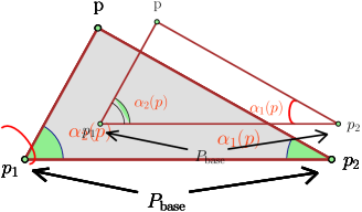
Figure 4.1: Example base angles when $k=3$

Observation 4.9 (Inclusion and base angles).

Let ${{B}}$ be a set of $k-1$ points in $\mathbb{R}^{k-1}$ all with their $(k-1)$th coordinate being zero, and let ${{p}}$ be an additional point with its $(k-1)$th coordinate being a positive number. Then, for a point ${{q}}\in\mathbb{R}^{k-1}$, we have that ${{q}}\in{{{{\triangle}}}}_{{{B}}\cup\left\{{{{p}}}\right\}}$ $\iff$ ${{\bm{\alpha}}}_{{{B}}}\left({{{q}}}\right)\leq{{\bm{\alpha}}}_{{{B}}}\left({{{p}}}\right)$ (i.e., $(\forall i:{{\alpha}}_{i}({{q}})\leq{{\alpha}}_{i}({{p}})$).

Lemma 4.10.

Given a set $n$ of $(k-1)$-simplices ${{\bm{\Delta}}}_{{G}}$ in $\mathbb{R}^{k-1}$, that all share common $k-1$ vertices, one can build a data structure of size $O(n\log^{k-1}n)$, such that given a query point ${{q}}\in\mathbb{R}^{k-1}$, one can compute $O(\log^{k-1}n)$ disjoint canonical sets, such that the union of these sets, is the set of all simplices in ${{\bm{\Delta}}}_{{G}}$ that contain ${{q}}$. The query time is $O(\log^{k-1}n)$.

Proof:

By a rigid transformation of the space, we can assume that ${{F}}$ is the hyperplane $x_{k-1}=0$, and furthermore, all the vertices of ${{\bm{\Delta}}}_{{G}}$ have $x_{k-1}\geq 0$ (we can handle the simplices $x_{k-1}\leq 0$ in a similar separate data structure). Let ${{P}}$ be the vertices of ${{\bm{\Delta}}}_{{G}}$ not lying on ${{F}}$. We generate the corresponding set of base angles ${{P}}_{{{\!\measuredangle}}}=\left\{{{\bm{\alpha}}}_{{{B}}}\left({{{p}}}\right)\;\middle|\;{{p}}\in{{P}}\right\}.$ Preprocess this set for orthogonal range searching, say, using range-trees [BCKO08]. Given a query point ${{q}}$, by Observation 4.9, the desired simplices correspond to all points in ${{p}}\in{{P}}$, such that ${{\bm{\alpha}}}_{{{B}}}\left({{{p}}}\right)\geq{{\bm{\alpha}}}_{{{B}}}\left({{{q}}}\right)$, which is an unbounded box query in the range tree of ${{P}}_{{{\!\measuredangle}}}$, with the aforementioned performance.  

Lemma 4.11.

The data structure of Lemma 4.10 can be used to report all simplices that contain a specific point ${{p}}$, and do not contain another point ${{p}}^{\prime}$, which is vertically above ${{p}}$ (i.e., the same point with larger $(k-1)$th coordinate). This corresponds to $k$ (possibly unbounded) box queries instead of quadrant query in the orthogonal data structure. The query time and number of canonical sets will be multiplied by at most $k$. The space bound remains the same. Moreover, we ensure these set of $k$ boxes are disjoint.

Proof:

If ${{p}}^{\prime}$ is vertically above ${{p}}$, we have that ${{\bm{\alpha}}}_{{{B}}}\left({{{p}}^{\prime}}\right)\geq{{\bm{\alpha}}}_{{{B}}}\left({{{p}}}\right)$. Let us denote ${{\bm{\alpha}}}_{{{B}}}\left({{{p}}}\right)$ by $\bm{\alpha}$ and ${{\bm{\alpha}}}_{{{B}}}\left({{{p}}^{\prime}}\right)$ by $\bm{\alpha}^{\prime}$. For $i=1,\ldots,k-1$, the algorithm would issue the box query

$$[\alpha_{1}^{\prime},\infty],[\alpha_{2}^{\prime},\infty],\cdots,[\alpha_{i-1}^{\prime},\infty],[\alpha_{i},\alpha_{i}^{\prime}],[\alpha_{i+1},\infty],\cdots,[\alpha_{k-1}^{\prime},\infty]$$

It is easy to verify that these boxes are disjoint and their union will correspond to all simplices that contain ${{p}}$ but not ${{p}}^{\prime}$. As each of these boxes correspond to polylogarithmic number of canonical sets, in total there are $O(k\log^{k-1}n)$ canonical sets.  

4.2.2 Data structure and correctness

Remark 4.12.

For a set of points ${{P}}$ and a base set ${{B}}$, consider the set of positive halfspaces (the positive bouquet) ${{\mathrm{bqt}^{+}}}\left({{{B}},{{P}}}\right)=\left\{{{\mathsf{f}}}^{+}\left({{{B}},{{p}}}\right)\;\middle|\;{{p}}\in{{P}}\setminus{{B}}\right\}.$ We can preprocess such a set for ANN queries readily, by using the data structure of Lemma 3.5. The only modification is that for every positive flat we assign one vector (in the positive direction), instead of two vectors in both directions which we put in the data structure of Section 3.2.

Preprocessing. The algorithm computes the set of canonical simplices ${{\bm{\Delta}}}_{{G}}$, see Eq. (4.2). Next, the algorithm builds the data structure of Lemma 4.10 for this set of simplices. For each canonical set ${{V}}$ in this data structure, for the corresponding set of original points, we build the data structure of Remark 4.12 to answer ANN queries on the positive bouquet ${{\mathrm{bqt}^{+}}}\left({{{B}},{{V}}}\right)$. (Observe that the total size of these canonical sets is $O(n\log^{k-1}n)$.)

Answering a query. Given a query point ${{q}}\in{{\Phi}}_{{{B}}}$, the algorithm computes its projection ${{q}}_{{B}}=\mathsf{nn}\left({{{q}},{{F}}}\right)$, where ${{F}}={{\mathsf{f}}}_{{{B}}}$. Let ${{r}}=\left\|{{q}}-{{q}}_{{B}}\right\|$ be the radius of ${{q}}$. The desired ANN distance is somewhere in the interval $[0,{{r}}]$, and the algorithm maintains an interval $[\alpha,\beta]$ where this distance lies, and uses binary search to keep pruning away on this interval, till reaching the desired approximation.

Observe that for every point ${{p}}\in{{P}}$, there is a critical value ${{\gamma}}\left({{{p}}}\right)$, such that for $x\geq{{\gamma}}\left({{{p}}}\right)$, the parameterized point ${{q}}_{{{G}}}\left({x}\right)$ is inside the simplex ${{{{\triangle}}}}_{{{G}}}\left({{{p}}}\right)$, and is outside if $x<{{\gamma}}\left({{{p}}}\right)$, see Definition 4.5. Note that this statement only holds for queries in ${{\Phi}}_{{{B}}}$ (otherwise it could have been false on simplices ${{{{\triangle}}}}_{{{B}}\cup\left\{{{{p}}}\right\}}$ with obtuse angles, see Remark 4.14 for handling the case of $q\notin{{\Phi}}_{{{B}}}$).

Now, by Lemma 4.11, we can compute a polylogarithmic number of canonical sets, such that the union of these sets, are (exactly) all the points with critical values in the range $[\alpha,\beta)$. As long as the number of critical values is at least one, we randomly pick one of these values (by sampling from the canonical sets – one can assume each canonical set is stored in an array), and let $\gamma$ be this value. We have to decide if the desired ANN is smaller or larger than $\gamma$. To this end, we compute a representation, by polylogarithmic number of canonical sets, of all the points of ${{P}}$ such that their simplex contains the parameterized point ${{q}}_{{{G}}}\left({\gamma}\right)$, using Lemma 4.10. For each such canonical set, the algorithm computes the approximate closest positive halfflat, see Remark 4.12. Let $\tau$ be the minimum distance of such a halfflat computed. If this distance is smaller than $\gamma$, then the desired ANN is smaller than $\gamma$, and the algorithm continues the search in the interval $[\alpha,\gamma)$, otherwise, the algorithm continues the search in the interval $[\gamma,\beta)$.

After logarithmic number of steps, in expectation, we have an interval $[\alpha^{\prime},\beta^{\prime})$, that contains no critical value in it, and the desired ANN distance lies in this interval. We compute the ANN positive flats for all the points that their parameterized simplex contains ${{q}}_{{{G}}}\left({\beta^{\prime}}\right)$, and we return this as the desired ANN distance.

Correctness. For the sake of simplicity, we first assume the ANN data structure returns the exact nearest-neighbor. Lemma 4.6 (A) readily implies that whatever simplex is being returned, its distance from the query point is the closeset, as claimed by the data structure. The other direction is more interesting – consider the unknown point ${{p}}_{k}$, such that the (desired) nearest point to the query point lies in the interior of the simplex ${{{{\triangle}}}}_{{{B}}\cup\left\{{{{p}}_{k}}\right\}}$ (we made this assumption at the beginning of Section 4.2). Lemma 4.6 (B) implies that the distance to this simplex is always going to be inside the active interval, as the algorithm searches (if not, then the algorithm had found even closer simplex, which is a contradiction).

To adapt the proof to the approximate case, suppose that the data structure of Remark 4.12 returns a $(1+\varepsilon)$ approximate nearest neighbor. Consider some iteration of the algorithm. Let ${{U}}\subseteq{{P}}$ be the set of all points ${{p}}$ such that the simplex ${{{{\triangle}}}}_{{{G}}}\left({{{p}}}\right)$ contains ${{q}}_{{{G}}}\left({\gamma}\right)$, and let ${{X}}$ be the set of simplices ${{{{\triangle}}}}_{{{B}}\cup\left\{{{{p}}}\right\}}$ corresponding to the points in ${{U}}$, and ${{\mathcal{F}}}$ be the set of half-flats ${{\mathsf{f}}}^{+}\left({{{B}},{{p}}}\right)$ corresponding to the points in ${{U}}$.

Suppose that $\ell^{*}$ is the minimum distance of the half-flats in ${{\mathcal{F}}}$ to the query, and let $\tau$ be the distance of the half-flat reported by the ANN data structure to the query. Thus, we have $\tau\leq\ell^{*}(1+\varepsilon)$. Note that, if $\tau<\gamma$, the optimal distance $\ell^{*}$ is also less than $\gamma$ and recursing on the interval $[\alpha,\gamma)$ works as it satisfies the precondition. However, if $\tau\geq\gamma$, then either $\ell^{*}\geq\gamma$ as well, in which case the recursion would work for the same reason, or $\ell^{*}<\gamma\leq\tau\leq\ell^{*}(1+\varepsilon)$.

In the latter case, let ${{p}}$ be the reported point corresponding to $\tau$. We know that the distance of the query to the half-flat ${{\mathsf{f}}}^{+}\left({{{B}},{{p}}}\right)$ is $\tau$ which is at most $\ell^{*}(1+\varepsilon)$. Now, if the simplex ${{{{\triangle}}}}_{{{G}}}\left({{{p}}}\right)$ contains the point ${{q}}_{G}(\tau)$, as well, then the distance of the query to the simplex ${{{{\triangle}}}}_{{{B}}\cup\left\{{{{p}}}\right\}}$ is equal to its distance to the half-flat ${{\mathsf{f}}}^{+}\left({{{B}},{{p}}}\right)$ which is $\tau\leq\ell^{*}(1+\varepsilon)$. Therefore, we can assume that ${{q}}_{G}(\tau)$ is outside of the simplex ${{{{\triangle}}}}_{{{G}}}\left({{{p}}}\right)$. However in this case, we get that the distance of the query to the simplex ${{{{\triangle}}}}_{{{B}}\cup\left\{{{{p}}}\right\}}$ is

$$\rho ={{\mathsf{d}}}({{q}},{{{{\triangle}}}}_{{{B}}\cup\left\{{{{p}}}\right\}})={{\mathsf{d}}}({{q}}_{{{H}}}\left({\tau}\right),{{{{\triangle}}}}_{{{G}}}\left({{{p}}}\right))\leq{{\mathsf{d}}}({{q}}_{{{H}}}\left({\tau}\right),{{q}}_{{{G}}}\left({\gamma}\right))=\sqrt{\tau^{2}+{{\mathsf{d}}}({{q}}_{G}(\tau),{{q}}_{G}(\gamma))^{2}}$$

$$=\sqrt{\tau^{2}+(\sqrt{{{r}}^{2}-\gamma^{2}}-\sqrt{{{r}}^{2}-\tau^{2}})^{2}}\leq\sqrt{\tau^{2}+\tau^{2}-\gamma^{2}}\leq\ell^{*}\sqrt{2(1+\varepsilon)^{2}-1}<\ell^{*}(1+2\varepsilon),$$

using ${{q}}_{{{G}}}\left({\gamma}\right)\in{{{{\triangle}}}}_{{{G}}}\left({{{p}}}\right)$, Eq. (4.1), and $\gamma\leq\tau\leq{{r}}$. The above implies that the distance of the query to the simplex ${{{{\triangle}}}}_{{{B}}\cup\left\{{{{p}}}\right\}}$ is a good approximation to the distance to the closest simplex. Thus, it is sufficient to modify the algorithm so that at each iteration, it checks the distance of simplex it finds to the query, and reports the best one found in all iterations.

Query time. In order to sample a value from $[\alpha,\beta)$ the algorithm uses Lemma 4.11 which has running time of $O(k\log^{k-1}n)$. Moreover, the algorithm performs $O(\log^{k-1}n)$ ANN queries in each iteration of the search corresponding to Lemma 4.10. As the search takes $O(\log n)$ iterations in expectation (and also with high-probability), the query time is $O({{T_{Q}}}\left({n,\varepsilon}\right)\log^{k}n)$. Note that this assumes $k$ is smaller than ${{T_{Q}}}\left({n,\varepsilon}\right)$ which holds as we are working in a low sparsity regime.

Lemma 4.13 (Approximate nearest induced page).

Given a set ${{P}}$ of $n$ points in $\mathbb{R}^{d}$, a set ${{B}}$ of $k-1$ points, and a parameter $\varepsilon>0$, one can preprocess them, such that given a query point, the algorithm computes an $(1+\varepsilon)$-ANN to the closest page in ${{\bm{\Delta}}}\left({{{B}},{{P}}}\right)$, see Definition 4.7. This assumes that (i) the nearest point to the query lies in the interior of the nearest page, and (ii) ${{q}}\in{{\Phi}}_{{{B}}}$. The algorithm space and preprocessing time is $O({{{S}}}\left({n,\varepsilon}\right)\log^{k}n)$, and the query time is $O({{T_{Q}}}\left({n,\varepsilon}\right)\log^{k}n)$.

4.3 Result: nearest induced simplex

The idea is to use brute-force to handle the distance of the query to the $\leq(k-2)$-simplices induced by the given point set which takes $O(n^{k-1})$ time. As such, the remaining task is to handle the $(k-1)$-simplices, and thus we can assume that the nearest point to the query lies in the interior of the nearest simplex, as desired by Lemma 4.13. To this end, we generate the $\binom{n}{k-1}=O(n^{k-1})$ choices for ${{B}}\subseteq{{P}}$, and for each one of them we build the data structure of Lemma 4.13, and query each one of them, returning the closet one found.

Remark 4.14.

Note that for a set of $k$ points ${{X}}\subset_{k}{{P}}$, if the projection of the query onto the simplex ${{{{\triangle}}}}_{A}$ falls inside the simplex, i.e. ${{q}}\in{{\Phi}}_{A}$, then there exists a subset of $k-1$ points ${{B}}\subset_{k-1}{{X}}$ such that the projection of the query onto the simplex ${{{{\triangle}}}}_{{{B}}}$ falls inside the simplex, i.e., ${{q}}\in{{\Phi}}_{{{B}}}$. Therefore, either the brute-force component of the algorithm finds an ANN, or there exists a set ${{B}}$ for which the corresponding data structure reports the correct ANN.

We thus get the following result.

Theorem 4.15 (Convex SLR).

Given a set ${{P}}$ of $n$ points in $\mathbb{R}^{d}$, and parameters $k$ and $\varepsilon>0$, one can preprocess them, such that given a query point, the algorithm can compute a $(1+\varepsilon)$-ANN to the closest $(k-1)$-simplex in ${{\bm{\Delta}_{k}\left({{{P}}}\right)}}$, see Definition 2.5. The algorithm space and preprocessing time is $O(n^{k-1}{{{S}}}\left({n,\varepsilon}\right)\log^{k}n)$, and the query time is $O(n^{k-1}{{T_{Q}}}\left({n,\varepsilon}\right)\log^{k}n)$.

5 Offline nearest induced segment problem

In this section, we consider the offline variant of the convex SLR problem, for the case of $k=2$. We present an algorithm which achieves constant factor approximation and has sub-quadratic running time.

Input & task. We are given a set of $n$ points ${{P}}=\left\{{{{p}}_{1},\cdots,{{p}}_{n}}\right\}$, along with the query point ${{q}}$, and a parameter $\varepsilon>0$. The task is to find the (approximate) closest segment ${{p}}_{i}{{p}}_{j}$ to the query point ${{q}}$, where ${{p}}_{i},{{p}}_{j}\in{{P}}$.

Notation.Fix a point ${{q}}$, and let $r>0$ be a parameter. For the sphere ${{\mathbb{S}}}={{\mathbb{S}}}\left({{{q}},r}\right)$, and a point ${{y}}\in\mathbb{R}^{d}$, let ${{{y}}}_{|{{\mathbb{S}}}}$ be the intersection point of $\mathrm{line}\left({{{y}},{{q}}}\right)$ with the sphere ${{\mathbb{S}}}$ that is closer to ${{y}}$. The other intersection point is the spherical reflection of ${{y}}$, and is denoted by $\mathrm{ref}\left({{{y}}}\right)={\left({{{q}}-({{y}}-{{q}})}\right)}_{|{{\mathbb{S}}}}$.

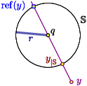
Figure 5.1:

Algorithm. The algorithm picks a value $r>0$ (any value works), and let ${{\mathbb{S}}}={{\mathbb{S}}}\left({{{q}},r}\right)$. Let ${{V}}=\{{{{p}}}_{|{{\mathbb{S}}}}\;|\;{{p}}\in{{P}}\}$ be the spherical projection of ${{P}}$ on ${{\mathbb{S}}}$. Next, the algorithm builds a data structure ${{\mathcal{D}}}$ for answering $(1+\varepsilon)$-ANN queries on ${{V}}$.

Now, the algorithm queries this data structure $n$ times. For each point ${{p}}_{i}\in{{P}}$, let ${{p}}_{i}^{\prime}=\mathrm{ref}\left({{{p}}_{i}}\right)$ be the spherical reflection of ${{p}}_{i}$. The algorithm queries the data structure ${{\mathcal{D}}}$ for the point ${{p}}_{i}^{\prime}$, and let ${{v}}_{i}\in{{V}}$ be the approximate nearest neighbor of ${{p}}_{i}^{\prime}$. Let $\widehat{{{p}}_{i}}$ be the original point of ${{P}}$ that induced the point ${{v}}_{i}$. The algorithm then computes the distance of the query ${{q}}$ to the segment ${{p}}_{i}\widehat{{{p}}_{i}}$ to see if it improves the closest segment found so far.

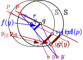
Figure 5.2:

5.1 Correctness

For points ${{p}},{{y}}\in\mathbb{R}^{d}$, let $r=\left\|{{q}}-{{p}}\right\|$, and let

$$f({{y}})={{\mathsf{d}}}({{q}},{{p}}{{y}})\qquad\text{ and }\qquad g({{y}})=\|{\mathrm{ref}\left({{{p}}}\right)-{{{y}}}_{|{{\mathbb{S}}}}}\|,$$

see Figure 5.2 (note, that ${{\mathbb{S}}}$ is determined by the value of $r$ specified). The task at hand is to approximate the minimum of $f({{y}})$, over all ${{p}},{{y}}\in{{P}}$. The key observation is that $g({{y}})$ is a good approximation to $f({{y}})$.

Lemma 5.1.

Using the above notations, consider a point ${{y}}\in\mathbb{R}^{d}$, such that $\left\|{{y}}-{{q}}\right\|\geq r$. Then, $f({{y}})\leq g({{y}})\leq 2f({{y}})$.

   (A) (B)

figure

Proof:

As ${{y}}$ moves away from ${{q}}$ along $\mathrm{line}\left({{{q}},{{y}}}\right)$, the quantity $g({{y}})$ remains the same, while $f({{y}})$ increases.

In particular, let $\ell$ be the limit line of $\mathrm{line}\left({{{p}},{{y}}}\right)$, as ${{y}}$ moves to infinity. Let ${{u}}$ be a point in distance $r$ along $\ell$ from ${{p}}$, see Figure 5.1 (A). Clearly, the two triangles $\triangle{{p}}{{q}}{{u}}$ and $\triangle{{q}}\mathrm{ref}\left({{{p}}}\right){{{y}}}_{|{{\mathbb{S}}}}$ are the same up to translation. As such, $f({{y}})$ is bounded by the height of ${{q}}$ in $\triangle{{p}}{{q}}{{u}}$, as this is the limit value of $f({{y}})$ as ${{y}}$ moves to infinity. Thus, $f({{y}})$ is bounded by the length of the edge ${{u}}{{q}}$, which is equal to $g({{y}})$. Implying that $f({{y}})\leq g({{y}})$.

Similarly, $f({{y}})$ is minimized when ${{y}}\in{{\mathbb{S}}}\left({{{q}},r}\right)$; that is, $\left\|{{q}}-{{y}}\right\|=r$, see Figure 5.1 (B). Letting $\alpha=\measuredangle{{q}}{{p}}{{y}}$, we have that $f({{y}})=r\sin\alpha$ and $g({{y}})=2r\sin(\alpha)=2f({{y}}),$ which implies the claim.  

Lemma 5.2.

The above algorithm $2(1+\varepsilon)$-approximates the closest induced segment of ${{P}}$.

Proof:

Let ${{p}}{{y}}$ be the two points such that the segment ${{p}}{{y}}$ is the closest to ${{q}}$ among all the induced segments of ${{P}}$. Assume that $\left\|{{q}}-{{p}}\right\|\leq\left\|{{q}}-{{y}}\right\|$. Note, that the algorithm works the same for any value of $r$. Indeed, the point set ${{V}}$ scales up with the value of $r$, but the nearest-neighbor queries are also scaled accordingly, and the answers returned by the ANN data-structure are the same.

In particular, for the analysis, we set $r=\left\|{{q}}-{{p}}\right\|$. Assume ${{\mathcal{D}}}$ returned the point ${{{u}}}_{|{{\mathbb{S}}}}$, and as such, the data-structure computed the distance $\Delta={{\mathsf{d}}}({{q}},{{p}}{{u}})=f({{u}})$, while the desired distance is $\delta={{\mathsf{d}}}({{q}},{{p}}{{y}})=f({{y}})$. If $\delta\geq r/[2(1+\varepsilon)],$ then we are done as the algorithm always returns a distance $\leq r$ (since the point ${{p}}$ is in distance $r$ from ${{q}}$), and thus get the desired approximation. As such, assume that $\delta<r/[2(1+\varepsilon)]$. By Lemma 5.1, we have that $\delta=f({{y}})\leq g({{y}})\leq 2f({{y}})<r/(1+\varepsilon)$. As $g({{y}})=\|{\mathrm{ref}\left({{{p}}}\right)-{{{y}}}_{|{{\mathbb{S}}}}}\|$, and since we are using $(1+\varepsilon)$-ANN data-structure, we have that $g({{u}})=\|{\mathrm{ref}\left({{{p}}}\right)-{{{u}}}_{|{{\mathbb{S}}}}}\|\leq(1+\varepsilon)g({{y}})\leq r.$

If $\left\|{{q}}-{{u}}\right\|\geq r$, then Lemma 5.1 readily implies that $f({{u}})\leq g({{u}})\leq(1+\varepsilon)g({{y}})\leq 2(1+\varepsilon)f({{y}}),$ which implies the claim.

If $\left\|{{q}}-{{u}}\right\|<r$, then observe that $f({{u}})\leq f({{{u}}}_{|{{\mathbb{S}}}})$, as moving $u$ in the direction of vector from ${{u}}$ to ${{{u}}}_{|{{\mathbb{S}}}}$ only increases the distance of the segment ${{p}}{{u}}$ from ${{q}}$. As such, by the same argument as above, we have that $f({{u}})\leq f({{{u}}}_{|{{\mathbb{S}}}})\leq g({{u}})\leq(1+\varepsilon)g({{y}})\leq 2(1+\varepsilon)f({{y}}),$ as desired.  

We thus get the following.

Theorem 5.3.

Given a set ${{P}}$ of $n$ points in $\mathbb{R}^{d}$, a query point ${{q}}$, and a parameter $\varepsilon>0$, one can compute $2(1+\varepsilon)$-ANN to the closest induced segment by ${{P}}$. The algorithm uses $O({{{S}}}\left({n,\varepsilon}\right))$ space, and its running time is $O\left({n{{T_{Q}}}\left({n,\varepsilon}\right)+{{{S}}}\left({n,\varepsilon}\right)}\right)$, where ${{{S}}}\left({n,\varepsilon}\right)$ is the space and ${{T_{Q}}}\left({n,\varepsilon}\right)$ is the query time for a $(1+\varepsilon)$-ANN data-structure for $n$ points in $\mathbb{R}^{d}$.

In particular, using the ANN data-structure of [AI06] for the ANN in the Euclidean space, the resulting running time is $n^{1+O({1}/{(1+\varepsilon)^{2}})}$ (i.e., sub-quadratic in $n$).

Corollary 5.4.

In constant dimension, using the ANN data-structure of Arya et al. [AMN⁺98], Theorem 5.3 yields a data-structure with $O(n)$ preprocessing, and $O(n\log n+n/\varepsilon^{d})$ running time.

6 Conditional lower bound

In this section, we reduce the $k$-sum problem to offline variant of all of our problems, ANLIF, ANIF and ANIS problems, providing an evidence that the time needed to solve these problems is $\tilde{\Omega}(n^{k/2}/e^{k})$. In the $k$-sum problem, we are given $n$ integer numbers $a_{1},\cdots,a_{n}$. The goal is to determine if there exist $k$ numbers among them $a_{i_{1}},\cdots,a_{i_{k}}$ such that their sum equals zero. The problem is conjectured to require $\Omega(n^{\lceil k/2\rceil}/\log^{\Theta(1)}n)$ time, see [PW10], Section 5.

We reduce this problem as follows. Let ${{P}}=\left\{{v_{1},\cdots,v_{n}}\right\}$ be a set of $n$ vectors of dimension $k+1$. More precisely, each $v_{i}\in\mathbb{R}^{k+1}$ has its first coordinate equal to $a_{i}$ and all the other coordinates are $0$ except for one coordinate chosen uniformly at random from $\{2,\ldots,k+1\}$, whose value we set to $1$. The query is also a vector of dimension $(k+1)$ and is of the form ${{q}}=[0,1/k,1/k,\cdots,1/k]^{T}$. We query the point ${{q}}$ and let $v_{i_{1}},\cdots,v_{i_{k}}$ be the points corresponding to the approximate closest flat/simplex reported by the algorithm. We then check if $\sum_{j=1}^{k}a_{i_{j}}=0$, and if so, we report $\left\{{a_{i_{1}},\cdots,a_{i_{k}}}\right\}$. Otherwise, we report that no such $k$ numbers exist. Next, we prove the correctness via the following two lemmas.

Lemma 6.1.

If there is no solution to the $k$-sum problem, that is if there is no set $\left\{{i_{1},\cdots,i_{k}}\right\}$ such that $\sum_{j=1}^{k}a_{i_{j}}=0$, then the distance of the query to the closest flat/simplex is non-zero.

Proof:

Suppose that the distance of the query to the closest flat/simplex is zero. Thus, there exist $k$ vectors $v_{i_{1}},\cdots,v_{i_{k}}$ and the coefficients $c_{1},\cdots,c_{k}$, such that $c_{1}v_{i_{1}}+\cdots+c_{k}v_{i_{k}}=q$. Let $t_{1},\cdots,t_{k}$ be the coordinates ($t_{i}$ has value from $2$ to $(k+1)$) such that $v_{i_{j}}$ has nonzero value in its $t_{j}$th coordinate. Note that ${{q}}$ has exactly $k$ nonzero coordinates, and each $v_{i_{j}}$ has exactly one non-zero coordinate from $2$ to $(k+1)$th coordinates, and there are $k$ such vectors. Thus $t_{1},\cdots,t_{k}$ should be a permutation from $2$ to $k+1$. Therefore all $c_{j}$’s should be equal to $1/k$. Hence, we also have that $a_{i_{1}}+\cdots+a_{i_{k}}=0$ which is a contradiction. Therefore the lemma holds.  

Lemma 6.2.

If there exist $a_{i_{1}},\cdots,a_{i_{k}}$ such that $\sum_{j=1}^{k}a_{i_{j}}=0$, then with probability $e^{-k}$ the solution of the affine SLR/convex SLR/SLR would be a flat/simplex which contains the query ${{q}}$.

Proof:

We consider the sum of $\frac{1}{k}v_{i_{1}}+\cdots+\frac{1}{k}v_{i_{k}}$ and show that it equals ${{q}}$ with probability $e^{-k}$. Let $t_{j}$ be the position (from $2$ to $(k+1))$ of the coordinate with value $1$ in vector $v_{i_{j}}$. Then if $t_{1},\cdots,t_{k}$ is a permutation from $2$ to $k+1$, we have that $\sum_{j=1}^{k}\frac{1}{k}\cdot v_{i_{j}}=q$ and thus the solution of the affine SLR/convex SLR/SLR would contain ${{q}}$ (notice that the coefficients are positive and they sum to $1$, so they satisfy the required constraints). The probability that $t_{1},\cdots,t_{k}$ is a permutation is ${k!\over k^{k}}\approx{\sqrt{2\pi k}(k/e)^{k}\over k^{k}}\geq e^{-k}$.  

Therefore we repeat this process $e^{k}$ times, and if any of the reported flats/simplices contained the query point, then we report the corresponding solution $\left\{{a_{i_{1}},\cdots,a_{i_{k}}}\right\}$. Otherwise, we report that no such $a_{i_{1}},\cdots,a_{i_{k}}$ exists. This algorithm reports the answer correctly with constant probability by the above lemmas. Moreover as the algorithm needs to detect the case when the optimal distance is zero or not, this lower bound works for any approximation of the problem. Thus we get the following theorem.

Theorem 6.3.

There is an algorithm for the $k$-sum problem with the running time bounded by $O(e^{k})$ times the required time to solve any of the three variants of the approximate SLR problem.

7 Approximating the nearest induced segment

In this section, we consider the online / query variant of the ANIS problem for the case of $k=2$. That is, given a set of $n$ points ${{P}}\subset\mathbb{R}^{d}$, the goal is to preprocess ${{P}}$, such that given a query point ${{q}}$, one can approximate the closest segment formed by any of the two points in ${{P}}$ to ${{q}}$.

7.1 Approximating the nearest neighbor in a star

Here, we show how to handle the non-uniform star case – namely, we have a set of $n$ segments (of arbitrary length), all sharing an endpoint, and given a query point, we would like to compute quickly the ANN on the star to this query.

7.1.1 Preliminaries

Lemma 7.1.

Let ${{P}}=\left\{{{{p}}_{1},\ldots,{{p}}_{n}}\right\}$ be an ordered set of $n$ points in $\mathbb{R}^{d}$. Given a data structure that can answer $(1+\varepsilon)$-ANN queries for $n$ points in $\mathbb{R}^{d}$, with space ${{{S}}}\left({n,\varepsilon}\right)$ and query time ${{T_{Q}}}\left({n,\varepsilon}\right)$, then one can build a data structure, such that for any integer $i$ and a query ${{q}}$, one can answer $(1+\varepsilon)$-ANN queries on the prefix set ${{P}}_{i}=\left\{{{{p}}_{1},\ldots,{{p}}_{i}}\right\}$. The query time and space requirement becomes $O({{{S}}}\left({n,\varepsilon}\right)\log n)$ and $O({{T_{Q}}}\left({n,\varepsilon}\right)\log n)$, respectively.

Proof:

This is a standard technique used for example in building range trees [BCKO08]. Build a balanced binary tree over ${{P}}$, with the leafs of the tree ordered in the same way as in ${{P}}$. Build for any internal node in this tree, the ANN data structure for the canonical set of points stored in this subtree. Now, an $(i,{{q}})$-ANN query, can be decomposed into ANN queries over $O(\log n)$ such canonical sets. For each canonical set, the algorithm uses the ANN data structure built for it. The algorithm returns the best ANN found.  

Given a set of points ${{P}}$, and a base point ${{c}}$, its star is the collection of segments ${{\mathrm{star}}}\left({{{c}},{{P}}}\right)=\bigcup_{{{y}}\in{{P}}}{{c}}{{y}}$ as defined in Definition 2.4. The set of points in such a star at distance $r$ from ${{c}}$, is the set of points

$${{\circledcirc}}\left({{{c}},r,{{P}}}\right)=\left\{{{v}}\;\middle|\;\Bigl{.}{{y}}\in{{P}},\|{{c}}-{{y}}\|\geq r,\text{ and }{{v}}={{c}}{{y}}\cap{{\mathbb{S}}}\left({{{c}},r}\right)\right\},$$ (7.1)

where ${{\mathbb{S}}}\left({{{c}},r}\right)$ denotes the sphere of radius $r$ centered at ${{c}}$.

Lemma 7.2.

Let ${{c}}$ be a point, and let ${{P}}$ be a set of $n$ points in $\mathbb{R}^{d}$. Given a data structure that can answer $(1+\varepsilon)$-ANN queries for $n$ points in $\mathbb{R}^{d}$, with space ${{{S}}}\left({n,\varepsilon}\right)$ and query time ${{T_{Q}}}\left({n,\varepsilon}\right)$, then one can build a data structure, such that given a query point ${{q}}$ and radius $r$, one can answer $(1+\varepsilon)$-ANN queries on the set of points ${{\circledcirc}}\left({{{c}},r,{{P}}}\right)$ (see Eq. (7.1)). The query time and space bounds are $O({{{S}}}\left({n,\varepsilon}\right)\log n)$ and $O({{T_{Q}}}\left({n,\varepsilon}\right)\log n)$, respectively.

Proof:

Let ${{P}}=\left\{{{{p}}_{1},\ldots,{{p}}_{n}}\right\}$ be the ordering of ${{P}}$ such that the points are in decreasing distance from ${{c}}$. Let ${{V}}=\left\{{{{v}}_{1},\ldots,{{v}}_{n}}\right\}$, be the ordering of the direction vectors of the points of ${{P}}$, where ${{v}}_{i}=({{p}}_{i}-{{c}})/\left\|{{p}}_{i}-{{c}}\right\|$. Build the data structure of Lemma 7.1 on the (ordered) point set ${{V}}$.

Given a query point ${{q}}$, using a balanced binary search tree, find the maximal $i$, such that $\ell=\left\|{{c}}-{{p}}_{i}\right\|\geq r$. Compute the affine transformation ${{M}}\left({{{q}}}\right)=({{q}}-{{c}})/r$, and compute the $(1+\varepsilon)$-ANN to ${{M}}\left({{{q}}}\right)$ in ${{V}}_{i}$, and let ${{v}}_{j}$ be this point. The algorithm returns ${{p}}_{j}$ is the desired ANN.

To see why this procedure is correct, observe that ${{\circledcirc}}\left({{{c}},r,{{P}}_{i}}\right)={{\circledcirc}}\left({{{c}},r,{{P}}}\right)$, where ${{P}}_{i}=\left\{{{{p}}_{1},\ldots,{{p}}_{i}}\right\}$. Furthermore, ${{V}}_{i}=\left\{{{{v}}_{1},\ldots,{{v}}_{i}}\right\}={{M}}\left({{{\circledcirc}}\left({{{c}},r,{{P}}_{i}}\right)}\right)$. In particular, since ${{M}}$ is only translation and scaling, it preserves order between distances of pairs of points. In particular, if ${{y}}$ is the ANN to ${{q}}$ in ${{\circledcirc}}\left({{{c}},r,{{P}}}\right)$, then ${{M}}\left({{{y}}}\right)$ is an ANN to ${{M}}\left({{{q}}}\right)$ in ${{M}}\left({{{\circledcirc}}\left({{{c}},r,{{P}}}\right)}\right)={{V}}_{i}$, implying the correctness of the above.  

7.1.2 The query algorithm

The algorithm in detail.

We are given a set of $n$ points ${{P}}$ and a center point ${{c}}\in{{P}}$, and we are interested in answering $(1+\varepsilon)$-ANN queries on ${{\star}}={{\mathrm{star}}}\left({{{c}},{{P}}}\right)$.

Preprocessing. We sort the points of ${{P}}$ to be in decreasing distance from ${{c}}$, and let ${{P}}=\left\{{{{p}}_{1},\ldots,{{p}}_{n}}\right\}$ be the points in this sorted order. We build the data structure ${{\mathcal{D}}}$ of Lemma 7.2 for the points of ${{P}}$ to answer $(1+\varepsilon/4)$-ANN queries.

Answering a query. Given a query point ${{q}}$, let $r=\left\|{{q}}-{{c}}\right\|$. As a first step, we perform $(1+\varepsilon/4)$-ANN query on ${{P}}$. Next, let $r_{i}=i(\varepsilon^{2}/16)r$, for $i=1,\ldots,N=32/\varepsilon^{2}$. For each $i$, find the $(1+\varepsilon/4)$-ANN in the point set ${{\circledcirc}}\left({{{c}},r_{i},{{P}}}\right)$, using the data structure ${{\mathcal{D}}}$. Return the nearest point to ${{q}}$ found as the desired ANN.

7.1.3 Correctness

Observe that ${{\mathsf{d}}}({{q}},{{\star}})\leq r$, since ${{c}}\in{{P}}\subseteq{{\star}}={{\mathrm{star}}}\left({{{c}},{{P}}}\right)$.

Lemma 7.3.

If ${{\mathsf{d}}}({{q}},{{\star}})\geq r\sqrt{\varepsilon}/2$ then the above algorithm returns a point ${{p}}\in{{\star}}$, such that $\left\|{{q}}-{{p}}\right\|\leq(1+\varepsilon){{\mathsf{d}}}({{q}},{{\star}})$, for any $0<\varepsilon\leq 1$.

Proof:

Let $\ell={{\mathsf{d}}}({{q}},{{\star}})$. Consider the point set ${{U}}_{i}=\bigcup_{i=1}^{N}{{\circledcirc}}\left({{{c}},r_{i},{{P}}}\right)$. The algorithm effectively performs $(1+\varepsilon/4)$-ANN query over this point set. So, let ${{q}}^{\prime}=\mathsf{nn}\left({{{q}},{{\star}}}\right)$, and let ${{y}}\in{{P}}$ be the point, such that ${{q}}^{\prime}\in{{c}}{{y}}$.

By construction, there is a choice of $i$, and a point ${{u}}\in{{U}}_{i}\cap{{c}}{{y}}$, such that $\left\|{{u}}-{{q}}^{\prime}\right\|\leq(\varepsilon^{2}/16)r$. Namely, we have ${{\mathsf{d}}}({{q}},{{U}})\leq{{\mathsf{d}}}({{q}},{{\star}})+(\varepsilon^{2}/16)r$. As such, the $(1+\varepsilon/4)$-ANN point returned for ${{q}}$ in ${{U}}$, is in distance at most

$$(1+\varepsilon/4)\left\|{{q}}-{{u}}\right\| \leq(1+\varepsilon/4)\left({\bigl{.}\left\|{{q}}-{{q}}^{\prime}\right\|+(\varepsilon^{2}/16)r}\right)\leq(1+\varepsilon/4)\left\|{{q}}-{{q}}^{\prime}\right\|+(\varepsilon^{2}/8)r$$

$$\leq(1+\varepsilon/2){{\mathsf{d}}}({{q}},{{\star}}),$$

since ${{\mathsf{d}}}({{q}},{{c}}{{y}})={{\mathsf{d}}}({{q}},{{\star}})$.  

The above lemma implies that (conceptually) the hard case is when the ANN distance is small (i.e., $O(\sqrt{\varepsilon}r)$). The intuition is that in this case the (regular) ANN query on ${{P}}$ and ${{\circledcirc}}\left({{{c}},r,{{P}}}\right)$ would “capture” this distance, and returns to us the correct ANN. The following somewhat tedious lemma testifies to this effect.

Lemma 7.4.

Let ${{c}},{{q}}$ be two given points, where $r=\left\|{{q}}-{{c}}\right\|$, and let $0<\varepsilon\leq 1$ be a parameter. Consider a set of $n$ points ${{Z}}=\left\{{{{p}}_{1},\ldots,{{p}}_{n}}\right\}\subseteq{{\bm{b}}}\left({{{c}},r}\right)$, where ${{\bm{b}}}\left({{{c}},r}\right)$ denotes the ball centered at ${{c}}$ of radius $r$. Let ${{\star}}={{\mathrm{star}}}\left({{{c}},{{Z}}}\right)$, and assume that ${{\mathsf{d}}}({{q}},{{\star}})\leq r\sqrt{\varepsilon}/2$. Then, we have that ${{\mathsf{d}}}({{q}},{{Z}})\leq(1+\varepsilon/4){{\mathsf{d}}}({{q}},{{\star}}).$

Proof:

Observe that by definition ${{\mathsf{d}}}({{q}},{{\star}})\leq{{\mathsf{d}}}({{q}},{{Z}})$. Let ${{q}}^{\prime}=\mathsf{nn}\left({{{q}},{{\star}}}\right)$, and consider the clipped cone ${{C}}$ of all points ${{y}}\in{{Z}}$ in distance at most $r$ from ${{c}}$, such that $\measuredangle{{y}}\hskip 0.6pt{{c}}\hskip 0.6pt{{q}}\leq\phi=\sqrt{\varepsilon}/2$.

Assume that ${{q}}^{\prime}$ is in ${{C}}$. Then, there must be a point ${{y}}\in{{Z}}\cap{{C}}$ such that ${{q}}^{\prime}\in{{c}}{{y}}$. Observe that ${{\mathsf{d}}}({{q}},{{\star}})=\left\|{{q}}-{{q}}^{\prime}\right\|={{\mathsf{d}}}({{q}},{{c}}{{y}})$. If ${{\mathsf{d}}}({{q}},{{c}}{{y}})=\left\|{{q}}-{{y}}\right\|\geq{{\mathsf{d}}}({{q}},{{Z}})$, which implies that ${{\mathsf{d}}}({{q}},{{Z}})={{\mathsf{d}}}({{q}},{{\star}})$, and we are done.

As such, consider the case that ${{\mathsf{d}}}({{q}},{{c}}{{y}})<\left\|{{q}}-{{y}}\right\|$, which is depicted in Figure 7.1. Clearly, $\beta=\measuredangle{{q}}{{y}}{{c}}$ is minimized when $\left\|{{c}}-{{y}}\right\|=r$, and $\measuredangle{{y}}{{c}}{{q}}=\phi$. But then, this angle is equal to $\pi/2-\phi/2$, which implies that $\beta\geq\pi/2-\phi/2$.

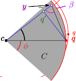
Figure 7.1: Illustration.

Now, $\|{{q}}-{{q}}^{\prime}\|=\|{{q}}-{{y}}\|\sin\beta$, and $\|{{q}}-{{y}}\|\leq 2r\sin(\phi/2)$. As such,

$$\Delta=\|{{q}}-{{y}}\|-\|{{q}}-{{q}}^{\prime}\|=\|{{q}}-{{y}}\|-\|{{q}}-{{y}}\|\sin\beta=\|{{q}}-{{y}}\|\left({\bigl{.}1-\sin\beta}\right).$$

In particular, we have ${1-\sin\beta}\leq{\Bigl{.}1-\sin(\pi/2-\phi/2)}={\Bigl{.}1-\cos(\phi/2)}\leq 1-(1-(\phi/2)^{2}/2)=\phi^{2}/8=\varepsilon/32,$ since $\cos(x)\geq 1-x^{2}/2$, for $x\leq\pi/4$. We conclude that $\Delta\leq(\varepsilon/32)\|{{q}}-{{y}}\|,$ which implies that $(1-\varepsilon/32)\left\|{{q}}-{{y}}\right\|\leq\|{{q}}-{{q}}^{\prime}\|.$ But then, we have ${{\mathsf{d}}}({{q}},{{Z}})\leq\left\|{{q}}-{{y}}\right\|\leq\frac{1}{1-\varepsilon/32}\|{{q}}-{{q}}^{\prime}\|\leq(1+\varepsilon/16){{\mathsf{d}}}({{q}},{{\star}}),$ implying the claim.

The remaining case is that ${{q}}^{\prime}$ is in ${{\bm{b}}}\left({{{c}},r}\right)\setminus{{C}}$. This implies that ${{\mathsf{d}}}({{q}},{{\star}})\geq{{\mathsf{d}}}({{q}},{{\bm{b}}}\left({{{c}},r}\right)\setminus{{C}})$, which is at least $r\sin\phi\geq r\sqrt{\varepsilon}/4$, since $\sin x\geq x/2$, for $x\leq 1/2$. But this is a contradiction to the assumption that ${{\mathsf{d}}}({{q}},{{\star}})\leq r\sqrt{\varepsilon}/2$.  

Lemma 7.5.

The query algorithm of Section 7.1.2 returns a $(1+\varepsilon)$-ANN to ${{\mathsf{d}}}({{q}},{{\star}})$, for any $\varepsilon\in(0,1)$.

Proof:

If ${{\mathsf{d}}}({{q}},{{\star}})\geq r\sqrt{\varepsilon}/2$ then the claim follows from Lemma 7.3. Otherwise, consider the point ${{p}}\in{{P}}$, such that $\mathsf{nn}\left({{{q}},{{\star}}}\right)$ lies on ${{c}}{{p}}$. If $\left\|{{c}}-{{p}}\right\|\leq r$, then by Lemma 7.4, the $(1+\varepsilon/4)$-ANN query on ${{\bm{b}}}\left({{{c}},r}\right)\cap{{P}}\subseteq{{P}}$ would return the desired ANN. (Formally, the result is worse by a factor of $(1+\varepsilon/4)$, which is clearly smaller than the desired threshold of $(1+\varepsilon)$.) Note, that the algorithm performs ANN query on ${{P}}$, and this resolves this case.

As such, we remain with the long case, that is $\left\|{{c}}-{{p}}\right\|>r$. But then, ${{q}}^{\prime}=\mathsf{nn}\left({{{q}},{{\star}}}\right)$ must lie inside ${{\bm{b}}}\left({{{c}},r}\right)$, where ${{\star}}={{\mathrm{star}}}\left({{{c}},{{P}}}\right)$. As such, in this case $\mathsf{nn}\left({{{q}},{{\star}}}\right)=\mathsf{nn}\left({{{q}},{{\mathrm{star}}}\left({{{c}},{{\circledcirc}}\left({{{c}},r,{{P}}}\right)}\right)}\right)$. As such, again by Lemma 7.4, the $(1+\varepsilon/4)$-ANN to ${{\circledcirc}}\left({{{c}},r,{{P}}}\right)$ is the desired approximation. Note, that the algorithm performs explicitly an ANN query on this point-set, implying the claim.  

Running time analysis and result. The algorithm built the data structure of Lemma 7.1 once, and we performed $O(1/\varepsilon^{2})$ ANN queries on it. This results in $O((\log n)/\varepsilon^{2})$ queries on the original ANN data structure. We thus conclude the following:

Lemma 7.6 (ANN in a star).

Let ${{P}}=\left\{{{{p}}_{1},\ldots,{{p}}_{n}}\right\}$ be a set of $n$ points in $\mathbb{R}^{d}$ and let $0<\varepsilon\leq 1$ be a parameter. Given a data structure that can answer $(1+\varepsilon)$-ANN queries for $n$ points in $\mathbb{R}^{d}$, using ${{{S}}}\left({n,\varepsilon}\right)$ space and ${{T_{Q}}}\left({n,\varepsilon}\right)$ query time, then one can build a data structure, such that for any query point ${{q}}$, it returns the $(1+\varepsilon)$-ANN to ${{q}}$ in ${{\star}}={{\mathrm{star}}}\left({{{c}},{{P}}}\right)$. The space needed is $O({{{S}}}\left({n,\varepsilon}\right)\log n)$, and the query time is $O({{T_{Q}}}\left({n,\varepsilon}\right)\varepsilon^{-2}\log n)$.

7.2 The result – approximate nearest induced segment

By building the data structure of Lemma 7.6 around each point of ${{P}}$, and querying each of these data structures, we get the following result.

Theorem 7.7.

Let ${{P}}=\left\{{{{p}}_{1},\ldots,{{p}}_{n}}\right\}$ be a set of $n$ points in $\mathbb{R}^{d}$ and let $0<\varepsilon\leq 1$ be a parameter. Given a data structure that can answer $(1+\varepsilon)$-ANN queries for $n$ points in $\mathbb{R}^{d}$, using ${{{S}}}\left({n,\varepsilon}\right)$ space and ${{T_{Q}}}\left({n,\varepsilon}\right)$ query time, then one can build a data structure, such that for any query point ${{q}}$, it returns a segment induced by two points of ${{P}}$, which is $(1+\varepsilon)$-ANN to the closest such segment. The space needed is $O({{{S}}}\left({n,\varepsilon}\right)n\log n)$, and the query time is $O({{T_{Q}}}\left({n,\varepsilon}\right)n\varepsilon^{-2}\log n)$.

Acknowledgements.

We thank Arturs Backurs for useful discussions on how the problem relates to the Hopcroft’s problem.

Appendix A Connection to Hopcroft’s problem

In the Hopcroft’s problem, we are given two sets $U$ and $V$, each consisting of $N$ vectors in $\mathbb{R}^{d}$ and the goal is to check whether there exists $u\in U$ and $v\in V$ such that $u$ and $v$ are orthogonal.

Given an instance of the Affine SLR with $n$ points and $k=4$, we proceed as follows. Suppose that the input is a set of $n$ points in $\mathbb{R}^{d}$ and the query is the origin 0. Moreover, suppose that $d=4$. So the goal is to decide whether there exist four points $a,b,c,d$ such that the three dimensional flat that passes through them also passes through the origin. This is equivalent to checking whether the determinant of the matrix which is formed by concatenating these four points as its columns, is zero or not. We can pre-process pairs of points to solve it fast.

Take all ${n\choose 2}$ pairs of points $a=(a_{1},a_{2},a_{3},a_{4})$ , $b=(b_{1},b_{2},b_{3},b_{4})$ and preprocess them by constructing a vector $u$ in 24 dimensional space such that $u=(a_{1}b_{2},-a_{1}b_{2},-a_{1}b_{3},a_{1}b_{3},\cdots,-a_{4}b_{3},a_{4}b_{3})$ and let $U$ be the set of such vectors $u$. Also, for each pair of points $c=(c_{1},c_{2},c_{3},c_{4})$ , $d=(d_{1},d_{2},d_{3},d_{4})$, we construct $v=(c_{3}d_{4},c_{4}d_{3},c_{2}d_{4},c_{4}d_{2},\cdots,c_{1}d_{2},c_{2}d_{1})$ and let $V$ be the set of ${n\choose 2}$ such vectors $v$. It is easy to check that the determinant is zero, if and only if the inner product of $u$ and $v$ is zero.

Thus, we have two collections $U$ and $V$ of $N={n\choose 2}$ vectors in $\mathbb{R}^{24}$ and would like to check whether there exists two points, one from each collection, that are orthogonal. So any lower bound better than $\omega(n^{k/2})=\omega(n^{2})$ would imply a super linear lower bound $\omega(N)$ for the Hopcroft’s problem.

References

- [AI06] A. Andoni and P. Indyk. Near-optimal hashing algorithms for approximate nearest neighbor in high dimensions. In Proc. 47th Annu. IEEE Sympos. Found. Comput. Sci. (FOCS), pages 459–468. IEEE Computer Society, 2006.
- [AMN+98] S. Arya, D. M. Mount, N. S. Netanyahu, R. Silverman, and A. Y. Wu. An optimal algorithm for approximate nearest neighbor searching in fixed dimensions. J. Assoc. Comput. Mach., 45(6):891–923, 1998.
- [BCKO08] M. de Berg, O. Cheong, M. van Kreveld, and M. H. Overmars. Computational Geometry: Algorithms and Applications. Springer-Verlag, Santa Clara, CA, USA, 3rd edition, 2008.
- [BHZM11] Ronen Basri, Tal Hassner, and Lihi Zelnik-Manor. Approximate nearest subspace search. IEEE Transactions on Pattern Analysis and Machine Intelligence, 33(2):266–278, 2011.
- [CDS98] Scott Shaobing Chen, David L. Donoho, and Michael A. Saunders. Atomic decomposition by basis pursuit. SIAM J. Sci. Comput., 20(1):33–61, 1998.
- [CRT06] E. J. Candes, J. Romberg, and T. Tao. Robust uncertainty principles: Exact signal reconstruction from highly incomplete frequency information. IEEE Trans. Inf. Theor., 52(2):489–509, February 2006.
- [DMA97] G. Davis, S. Mallat, and M. Avellaneda. Adaptive greedy approximations. Constructive Approx., 13(1):57–98, 1997.
- [Don06] David L. Donoho. Compressed sensing. IEEE Trans. Inf. Theor., 52(4):1289–1306, 2006.
- [ES95] J. Erickson and R. Seidel. Better lower bounds on detecting affine and spherical degeneracies. Discrete Comput. Geom., 13:41–57, 1995.
- [FKT15] Dean P. Foster, Howard J. Karloff, and Justin Thaler. Variable selection is hard. In Peter Grünwald, Elad Hazan, and Satyen Kale, editors, Proc. 28th Annu. Conf. Comp. Learn. Theo. (COLT), volume 40 of JMLR Proceedings, pages 696–709. JMLR.org, 2015.
- [IM98] P. Indyk and R. Motwani. Approximate nearest neighbors: Towards removing the curse of dimensionality. In Proc. 30th Annu. ACM Sympos. Theory Comput. (STOC), pages 604–613, 1998.
- [KOR00] E. Kushilevitz, R. Ostrovsky, and Y. Rabani. Efficient search for approximate nearest neighbor in high dimensional spaces. SIAM J. Comput., 2(30):457–474, 2000.
- [Mag02] Avner Magen. Dimensionality reductions that preserve volumes and distance to affine spaces, and their algorithmic applications. In International Workshop on Randomization and Approximation Techniques in Computer Science, pages 239–253. Springer, 2002.
- [Mah15] Sepideh Mahabadi. Approximate nearest line search in high dimensions. In Proc. 26th ACM-SIAM Sympos. Discrete Algs. (SODA), SODA ’15, pages 337–354. SIAM, 2015.
- [Nat95] Balas Kausik Natarajan. Sparse approximate solutions to linear systems. SIAM J. Comput., 24(2):227–234, April 1995.
- [PW10] Mihai Patrascu and Ryan Williams. On the possibility of faster SAT algorithms. In Moses Charikar, editor, Proc. 21st ACM-SIAM Sympos. Discrete Algs. (SODA), pages 1065–1075. SIAM, 2010.
- [Tib96] R. Tibshirani. Regression shrinkage and selection via the lasso. J. Royal Stat. Soc. Series B, 58(1):267–288, 1996.
- [Tib11] Robert Tibshirani. Regression shrinkage and selection via the lasso: a retrospective. J. Royal Stat. Soc. Series B, 73(3):273–282, 2011.
- [WYG+09] John Wright, Allen Y Yang, Arvind Ganesh, Shankar S Sastry, and Yi Ma. Robust face recognition via sparse representation. IEEE Trans. Pattern Anal. Machine Intel., 31(2):210–227, 2009.