No Conclusive Evidence for Transits of Proxima b in MOST photometry

Abstract

The analysis of Proxima Centauri’s radial velocities recently led Anglada-Escudé et al. (2016) to claim the presence of a low mass planet orbiting the Sun’s nearest star once every 11.2 days. Although the a-priori probability that Proxima b transits its parent star is just 1.5%, the potential impact of such a discovery would be considerable. Independent of recent radial velocity efforts, we observed Proxima Centauri for 12.5 days in 2014 and 31 days in 2015 with the MOST space telescope. We report here that we cannot make a compelling case that Proxima b transits in our precise photometric time series. Imposing an informative prior on the period and phase, we do detect a candidate signal with the expected depth. However, perturbing the phase prior across 100 evenly spaced intervals reveals one strong false-positive and one weaker instance. We estimate a false-positive rate of at least a few percent and a much higher false-negative rate of $20$-$40$%, likely caused by the very high flare rate of Proxima Centauri. Comparing our candidate signal to HATSouth ground-based photometry reveals that the signal is somewhat, but not conclusively, disfavored (1-2 $\sigma$) leading us to argue that the signal is most likely spurious. We expect that infrared photometric follow-up could more conclusively test the existence of this candidate signal, owing to the suppression of flare activity and the impressive infrared brightness of the parent star.

1 INTRODUCTION

Proxima Centauri is the Sun’s nearest stellar neighbor at a distance of 1.295 parsecs (van Leeuwen, 2007). Despite this, Proxima’s late spectral type (M5.5; Bessell 1991) makes it too faint to be seen by the naked eye ($V=11.1$; Jao et al. 2014), elucidating why this is not the easiest target in the search for extrasolar planets. This challenge is exacerbated by the activity of Proxima itself, being a classic flare star (Christian et al., 2004).

Nevertheless, Proxima is one of the best studied low-mass stars and its diminutive mass offers an enhanced radial velocity semi-amplitude, $K$, scaling as $M_{\star}^{-2/3}$. Accordingly, translating the same planet from the Sun to Proxima would cause $K$ to increase by a factor of four. Early radial velocity campaigns, such as those of Endl & Kürster (2008) and Zechmeister et al. (2009) found no signals at the few m s^-1 level, ruling out Super-Earths in the habitable-zone.

The hunt for planets around our nearest star fell to the sidelines in the following years, notably during the era of NASA’s Kepler Mission. With thousands of planetary candidates detections pouring in (Batalha et al., 2013), the exoplanet community reasonably focussed on these immediate discoveries. Although only a few thousand M-dwarfs were observed by Kepler (out of $\sim$200,000 targets), the Kepler results ultimately rekindled our team’s interest in the prospect of planets around Proxima.

First, the discovery of a planetary system around one of Kepler’s lowest mass stars, Kepler-42 (M5 dwarf), Muirhead et al. (2012) illustrated a putative template for what a potential planetary system around Proxima could resemble. Notably, the planets were all sub-Earth sized, and would thus have eluded the radial velocity search efforts of Endl & Kürster (2008) and Zechmeister et al. (2009), should similar planets orbit Proxima. More over, the planets were at extreme proximity to the star, with periods ranging from 0.45 d to 1.86 d, leading to sizable geometric transit probabilities. Indeed, should Proxima harbor a Kepler-42 like system, the transit probability would be $\sim$10%.

Second, Kepler occurrence rate statistics showed that planets around early M-dwarfs are very common, with an average of $(2.5\pm 0.2)$ planets per star (Dressing & Charbonneau, 2015). Radial velocity campaigns come to similar conclusions, finding evidence for at least one planet per M-dwarf (Tuomi et al., 2014). Together then, this implies that Proxima not only has an excellent chance of harboring a planetary system but such planets have a reasonable probability of transiting and producing mmag level signals. These arguments inspired our team to conduct a transit survey of Proxima starting in 2014 with the Microwave and Oscillations of Stars (hereafter MOST) telescope.

MOST is a 53 kg satellite in Low Earth Orbit (LEO) with a 15 cm aperture visible band camera (35-750 nm). MOST is able to deliver mmag level photometry (for $V\lesssim 12$) at high cadence over several weeks baselines, although observations are typically interrupted once per 101 minute orbit as the spacecraft passes behind the Earth. MOST has been successful in discovering several new transiting systems, such as 55 Cnc e (Winn et al., 2011), HD 97658 b (Dragomir et al., 2013) and most recently HIP 116454 b (Vanderburg et al., 2015). For Proxima Centauri, we estimated MOST should deliver $\sim 0.3$ mmag precision photometry on an hour timescale, making it well suited for detecting the 4.2 mmag transit expected to be caused by an Earth-sized planet and thus two seasons of observations were undertaken in 2014 and 2015.

Evidently, our team was not alone in returning to Proxima, with the Pale Red Dot campaign (PRD hereafter) conducting their own intensive search using radial velocities in 2016. By combining the PRD data with previous radial velocities, Anglada-Escudé et al. (2016) recently announced the detection of a 11.2 d planetary candidate- Proxima b. Since radial velocities do not reveal the inclination of the planetary orbit, only the minimum mass of Proxima b is presently known at $M_{P}\sin i=1.27_{-0.17}^{+0.19}$ $M_{\oplus}$. Since the transition from Terran (solid-like) to Neptunian worlds occurs at $(2.1\pm 0.6)$ $M_{\oplus}$ (Chen & Kipping, 2016), the compositional nature of Proxima b is presently ambiguous. If transits of Proxima b were observed, the inclination could be resolved, as well as offering the opportunity to further characterize this remarkable world.

In this work, we present the results of our search for transiting planets around Proxima Centauri with MOST photometry. We describe the observations and data treatment stages in Section 2 and our photometric model in Section 3. In Section 4, we present the results of a localized search using the reported Proxima b ephemeris, followed by two sets of tests in Sections 5&6. Finally, we discuss the constraints our data place on Proxima b in Section 7.

2 OBSERVATIONS

2.1 MOST Observations

MOST observed Proxima Centauri in May 2014 (beginning on HJD(2000) 2456793.18) for about 12.5 days. Proxima Centauri falls outside of the Continuous Viewing Zone of MOST ($-19^{\deg}$ to $+36^{\deg}$ in declination; see Walker et al. 2003) and can only be observed for a fraction of the satellite’s 101 min orbit. For this reason, and for other science queue considerations, data was collected for about 30% of each MOST orbit and was sampled at an average rate of 63.4 seconds. MOST again observed Proxima Centauri in May 2015 (starting on HJD(2000) 2457148.54), this time for a total of 31 days with extended coverage to almost 50% of every MOST orbit. Data were again sampled at an average rate of about 63 seconds.

Flux measurements were extracted from each image using aperture photometry techniques outlined by Rowe et al. (2006). Background counts, inter-pixel correlations, and pointing drifts were accounted for by subtracting polynomials fitted through correlations between the measured target flux and those parameters. Removal of stray Earth-shine onto the CCD was done by folding the time series at the orbital period of MOST and subtracting a running mean through 30 orbital bins. Any remaining statistical outliers were removed, resulting in $\sim$2600 individual time series measurements from the 2014 data set and $\sim$13000 data points from 2015.

The time series was then inspected for flare-like events using v1.3.11 of the flare-finding suite FBEYE from Davenport et al. (2014). The results of this exercise are discussed in detail in the accompanying paper of Davenport et al. (2016), but for the purposes of this work these points are removed in all subsequent analyses of the photometry. The location of these events are highlighted in Figure 1.

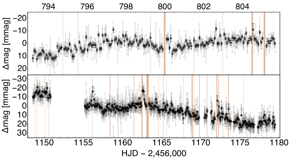
Figure 1: Corrected photometric observations of Proxima with MOST in 2014 (top) and 2015 (bottom) shown with 5$\times$cadence binning ($\sim 5.3$ minutes). Each orbital visit of MOST is binned together in black. The vertical colored regions denote regions ignored in this work, since flares were identified by Davenport et al. (2016).

2.2 Time-Correlated Structure and Trends

After correcting the photometry and removing the flares, it is clear that our MOST data exhibits time-correlated structure in both seasons (see Figure 1 and Table 1). Long-term trends are pronounced in both seasons, with 2014 displaying a slow brightness increase along with a sinusoidal-like few mmag variation on the timescale of a week. In 2015, the structure appears more complex and exhibits a slow brightness decrease. These trends are not seen in any of the comparison stars and thus we identify them as being astrophysical in nature.

The slow brightness trends may be associated with the claimed 83 d rotation period of Proxima Centauri (Benedict et al., 1998). The remaining, and quite pronounced, structure may be a result of frequent flaring (Davenport et al., 2016) and associated corononal mass ejections, as well as magnetic activity such as evolving spots, plages and networks.

Interpreting the origin of the observed structure is beyond the scope of this work, for which this structure represents a impediment in our ability to detect putative transits of Proxima.

Table 1: Reduced MOST photometry used in this work, excluding times afflicted by large flares. A portion of the table is shown here, the full version is available in the electronic version of the paper and at this URL.

HJDUTC - 2,451,545	$\Delta$mag	Uncertainty
5248.197851471566	0.0118	0.0030
5248.200048126498	0.0116	0.0030
5248.259628134210	0.0028	0.0026
5248.262194952687	0.0092	0.0030
5248.270990357013	0.0065	0.0030
5248.329765768074	0.0072	0.0026
5248.332326375948	0.0054	0.0030
5248.399228360851	0.0155	0.0030
⋮	⋮	⋮

2.3 Gaussian Process (GP) Regression

In order to search for transits, the structure and trends present in our data require modeling. For reasons described in what follows, we elected to use Gaussian Process (GP) regression to model out this structure. Here, one assumes the data is distributed around the transit model as a multivariate Gaussian including off-diagonal elements within its covariance matrix, $\boldsymbol{\Sigma}$. This eliminates the assumption of independent uncertainties and allows each point in the time series to have some degree of correlation with every other point. The log-likelihood function, used for subsequent regression, may be written as

$$\log\mathcal{L} =-\tfrac{1}{2}\mathbf{r}^{T}\boldsymbol{\Sigma}^{-1}\mathbf{r}-\tfrac{1}{2}\log\mathrm{det}\boldsymbol{\Sigma}-\tfrac{n}{2}\log 2\pi,$$ (1)

where $\mathbf{r}$ is a vector of the residuals between the transit model and the data. The very large number of covariance matrix elements are a-priori unknown to us, but GPs model the covariance matrix with some assumed smooth, functional form, known as the kernel. The kernel, $\mathbf{K}$, is described by one or more hyper-parameters, $\boldsymbol{\theta}_{\mathrm{hyper}}$, which are freely explored along with the usual model parameters, $\boldsymbol{\theta}_{\mathrm{transit}}$, during the fitting procedure.

GPs have emerged as one of the most popular and successful methods of modeling time correlated noise in the analysis of transit photometry (Gibson et al., 2012; Evans et al., 2015; Berta-Thompson et al., 2015) and are appealing for their ability to model complex structure with relatively few new regression parameters. However, inverting the covariance matrix at each realization is computationally expensive and typically GPs are computationally prohibitive for $n\gtrsim\mathcal{O}[10^{3}]$ data points, which is particularly relevant in this work given that we have over $10^{4}$ photometric measurements.

2.4 Binning and Kernel Selection

To overcome the computational challenge of inverting the covariance matrix, one may first apply modest binning to the time series. Ideally, the relevant correlation time scale(s) should be significantly greater than the time scale used for binning, such that correlations are preserved.

The native cadence of our photometric measurements is 63.5 seconds and after removing outliers and flares, we have 2461 data points in the 2014 season and 11473 points in 2015. We first assume the kernel parameters for each season are wholly independent, given the large change in time. We then focus on the null model of a transit-free case, where the data is solely described by an offset parameter, $a$, and the GP. Accordingly, the 2014 season can be treated independent of 2015.

We found that 2461 data points was not a computationally prohibitive number of points for GP regression, which allows us to directly compare the inferred GP kernel parameters between the binned and unbinned data. We set a binning time scale equal to 317.5 seconds (equivalent to 5 consecutive cadences), or approximately five minutes, and employ temporal windows for the binning rather than $N$-point binning, due to the considerable number of data gaps present. For the GP kernel, we adopted the popular Matérn-3/2 kernel given by

$$\mathbf{K}_{i,j}(\alpha,l) =\alpha^{2}\Bigg{(}1+\frac{\sqrt{3}|t_{i}-t_{j}|}{l}\Bigg{)}\exp\Bigg{(}-\frac{\sqrt{3}|t_{i}-t_{j}|}{l}\Bigg{)},$$ (2)

where $l$ controls the time scale of correlations and $\alpha$ controls the magnitude. The full covariance matrix, $\boldsymbol{\Sigma}$, is the sum of the matrix $\mathbf{K}$ and a diagonal matrix of the square of the measurement uncertainties. We then regressed both versions of the 2014 time series using MultiNest (Feroz & Hobson, 2008; Feroz et al., 2009) and computed parameter posteriors. The agreement between the two is excellent, with $a=0.79_{-0.57}^{+0.59}$ mmag from the unbinned data versus $a=0.78_{-0.58}^{+0.58}$ mmag using the binned. Similarly, the $l$ correlation time scale is almost identical- $l=130_{-15}^{+16}$ mins in the unbinned versus $l=130_{-15}^{+17}$ mins in the binned. Further, this time scale is much greater than the 5 minute binning time scale adopted, ensuring key correlations are not affected by the binning procedure.

For the 2015 data, we are unable to repeat this test given the much larger number of unbinned points. However, regressing the same model and GP on the 2015 binned data reveals $l=269_{-15}^{+15}$ mins, which is again much greater than the binning time scale (in fact even more so than before). Accordingly, we conclude that the 5 minute binning procedure does not affect the GP inference nor should affect our ability to detect transits, given that such events occur on significantly longer time scales too. Our final binned time series includes 709 points in the 2014 season and 2850 points in 2015, which are the points plotted in gray in Figure 1.

Although we assumed a Matérn-3/2 kernel in these tests, several other commonly used kernels are investigated before continuing. We compared the Bayesian evidence (or marginal likelihood) resulting from re-fitting both seasons of data for a Matérn-3/2 kernel, Matérn-3/2 quasi-periodic kernel, a Matérn-5/2 kernel and a squared-exponential kernel. After conducting these fits on the 2014 unbinned, 2014 binned and 2015 binned data, with identical priors, we find in all cases that the Matérn-3/2 kernel is favored, as shown in Table 2. We therefore adopt the Matérn-3/2 kernel in all subsequent photometric analysis of Proxima Centauri and show this favored GP over-plotted with the data in Figure 2.

Table 2: Comparison of Bayesian evidences, $\mathcal{Z}$, for four commonly used kernel choices. The preferred model for each data set is emboldened.

Kernel	$\log\mathcal{Z}$
2014 unbinned
Squared-Exponential	$9856.304\pm 0.088$
Matérn-3/2	$\mathbf{9865.807\pm 0.083}$
Matérn-5/2	$9862.166\pm 0.085$
Quasi-periodic Matérn-3/2	$9865.513\pm 0.084$
2014 binned
Squared-Exponential	$2989.686\pm 0.088$
Matérn-3/2	$\mathbf{2998.977\pm 0.084}$
Matérn-5/2	$2995.398\pm 0.085$
Quasi-periodic Matérn-3/2	$2998.795\pm 0.084$
2015 binned
Squared-Exponential	$11192.194\pm 0.109$
Matérn-3/2	$\mathbf{11337.855\pm 0.100}$
Matérn-5/2	$11284.873\pm 0.102$
Quasi-periodic Matérn-3/2	$11337.101\pm 0.103$

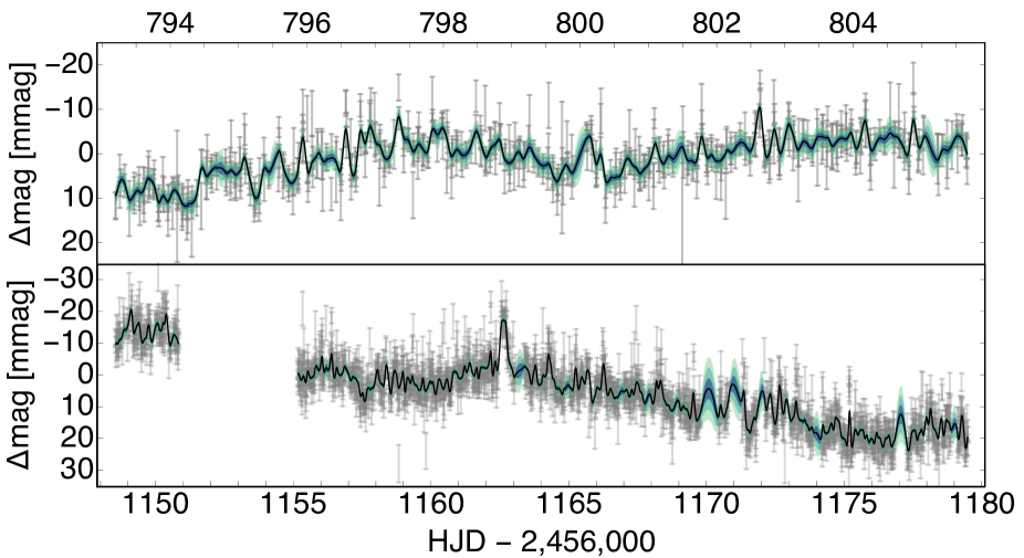
Figure 2: Corrected photometric observations of Proxima with MOST in 2014 (top) and 2015 (bottom) shown with 5$\times$cadence binning ($\sim 5.3$ minutes) with large flares excluded. The black line is the maximum likelihood fit of a GP using a Matérn-3/2 kernel, with the 0.5, 1.0 and 1.5 $\sigma$ confidence regions denoted by the gray regions (GP shown is from model $\mathcal{M}_{2}$).

3 PRIORS, MODELS & TESTS

3.1 Predicting the Transit Ephemeris

The radial velocity solution of Anglada-Escudé et al. (2016) provides joint posterior distributions for numerous parameters including the orbital period, $P$, and the mean anomaly at a reference time $t_{0}$, $M_{0}$. We first converted the $M_{0}$ column into a time of inferior conjunction, $t_{\mathrm{IC}}$, via Kepler’s equation. For low-eccentricity orbits, such as that of Proxima b ($e<0.3$ to 95% confidence; Anglada-Escudé et al. 2016), the time of transit minimum, $\tau$, is equal to the time of inferior conjunction (Kipping, 2011).

The time of inferior conjunction can be computed at any epoch of our choosing by adding on some integer number of periods. We therefore elected to calculate $t_{\mathrm{IC}}$ at every possible epoch from $-200$ to $+200$ orbital periods. For each realization, we computed the standard deviation of the resulting posterior and also the correlation with respect to the $P$ posterior samples. We found that both are minimized for $-65^{\mathrm{th}}$ epoch, for which $t_{\mathrm{IC}}=2,456,678.78\pm 0.56$ HJD. Both this term, and the orbital period of $P=(11.1856\pm 0.0013)$ d, are well approximated as two independent normal distributions.

3.2 Predicting the Radius

In order to guide our targeted search for transits of Proxima b, we first estimate the amplitude of the transit signal expected. If the mass of a planet is known, the radius can be predicted using an empirical mass-radius relation. In this work, we use the relation of Chen & Kipping (2016) which is probabilistic, includes freely inferred transitional regions and was calibrated on the widest range of data available.

If the planet is transiting, this imposes the condition that $b<1+p$. Given that Proxima b is an Earth-mass planet, we expect $p\simeq 0.06$ and thus $p\ll 1$. This allows us to write that a transiting Proxima b must satisfy

$$\cos i<\frac{1}{a_{R}}\frac{1-e^{2}}{1+e\sin\omega}.$$ (3)

Using the joint posterior distribution samples for $P$, $e$ and $\omega$ from Anglada-Escudé et al. (2016), this condition requires $i<89.1^{\circ}$ to 95.45% confidence. For any transiting planet then, the $\sin i$ effect on the true mass is much smaller than the present measurement uncertainty on $M_{P}\sin i$. Accordingly, we may simply adopt $M_{P}\simeq M_{P}\sin i$ in estimating the radius of a transiting Proxima b.

We now use the posterior samples of $M_{P}\sin i$ to estimate a probabilistic range for $R_{P}$ using the Forecaster code of Chen & Kipping (2016). This estimate accounts for the measurement uncertainty of Anglada-Escudé et al. (2016), the measurement uncertainties in the calibration of Chen & Kipping (2016) and the intrinsic dispersion in radii observed as a function of mass (Chen & Kipping, 2016). Under the assumption that Proxima b is transiting, we estimate that $R_{P}=1.06_{-0.11}^{+0.13}$ $R_{\oplus}$. Normalizing by the radius of the star (Demory et al., 2009), we predict $p=R_{P}/R_{\star}=0.0693_{-0.0083}^{+0.0095}$, which is well fit by a logistic distribution with shape parameters $\mu=0.069$ and $s=0.0051$. We also find that 99% of the posterior samples for $p$ satisfy $p<0.1$ and conservatively double this limit to $p<0.2$ as a truncation point to our prior. This also provides a cut-off for the impact parameter of $b<1.2$.

3.3 Models Considered and Associated Priors

We considered three different transit models in our targeted search for transits of Proxima b, where we varied the degree of prior information we used from the Anglada-Escudé et al. (2016) discovery. We label the models as $\mathcal{M}_{1}$, $\mathcal{M}_{2}$ and $\mathcal{M}_{3}$, where the subscript increases with increased use of prior information. These fits may be compared directly to the null fit of $\mathcal{M}_{0}$, where no transit is included and only the GP hyper-parameters, $\boldsymbol{\theta}_{\mathrm{hyper}}$, are fitted.

We list the priors used in Table 3, where it can be seen that the GP hyper-priors are identical in all fits. This allows us to compare the Bayesian evidences between each model to aid model selection. All three transit models used the normal prior on orbital period, otherwise the search would be blind rather than targeted. $\mathcal{M}_{2}$ uses an informative prior on the time of transit minimum, unlike $\mathcal{M}_{1}$. The final model, $\mathcal{M}_{3}$, also uses these period and phase informative priors plus an informative prior on the radius of the planet, as computed earlier in Section 3.2.

Table 3: Priors used in the targeted transit search of Proxima b, spanning four different models (each column). $\mathcal{U}$ denotes a uniform prior, $\mathcal{W}$ a wrap-around uniform, $\mathcal{J}$ a log-uniform, $\delta$ a Delta function prior and $\mathcal{X}$ a logistical distribution prior. We set the reference time to $t_{\mathrm{ref}}=2457165.385$ HJD.

Parameter	$\mathcal{M}_{0}$	$\mathcal{M}_{1}$	$\mathcal{M}_{2}$	$\mathcal{M}_{3}$
$a_{\mathrm{2014}}$ [mmag]	$\mathcal{U}[-10^{-2},10^{-2}]$	$\mathcal{U}[-10^{-2},10^{-2}]$	$\mathcal{U}[-10^{-2},10^{-2}]$	$\mathcal{U}[-10^{-2},10^{-2}]$
$\alpha_{\mathrm{2014}}$	$\mathcal{J}[-10^{-1},10^{1}]$	$\mathcal{J}[-10^{-1},10^{1}]$	$\mathcal{J}[-10^{-1},10^{1}]$	$\mathcal{J}[-10^{-1},10^{1}]$
$l_{\mathrm{2014}}$	$\mathcal{J}[-10^{-2},10^{0}]$	$\mathcal{J}[-10^{-2},10^{0}]$	$\mathcal{J}[-10^{-2},10^{0}]$	$\mathcal{J}[-10^{-2},10^{0}]$
$a_{\mathrm{2015}}$ [mmag]	$\mathcal{U}[-10^{-2},10^{-2}]$	$\mathcal{U}[-10^{-2},10^{-2}]$	$\mathcal{U}[-10^{-2},10^{-2}]$	$\mathcal{U}[-10^{-2},10^{-2}]$
$\alpha_{\mathrm{2015}}$	$\mathcal{J}[-10^{-1},10^{1}]$	$\mathcal{J}[-10^{-1},10^{1}]$	$\mathcal{J}[-10^{-1},10^{1}]$	$\mathcal{J}[-10^{-1},10^{1}]$
$l_{\mathrm{2015}}$	$\mathcal{J}[-10^{-2},10^{0}]$	$\mathcal{J}[-10^{-2},10^{0}]$	$\mathcal{J}[-10^{-2},10^{0}]$	$\mathcal{J}[-10^{-2},10^{0}]$
$p=(R_{P}/R_{\star})$	-	$\mathcal{J}[10^{-3},10^{-0.70}]$	$\mathcal{J}[10^{-3},10^{-0.70}]$	$\mathcal{X}[0.069,0.0050]$
$b$	-	$\mathcal{U}[0,1.2]$	$\mathcal{U}[0,1.2]$	$\mathcal{U}[0,1.2]$
$\tau$ [HJD-2,456,000]	-	$\mathcal{W}[t_{\mathrm{ref}},t_{\mathrm{ref}}+P]$	$\mathcal{N}[678.78,0.59]$	$\mathcal{N}[678.78,0.59]$
$P$ [days]	-	$\mathcal{N}[11.1856,0.0013]$	$\mathcal{N}[11.1856,0.0013]$	$\mathcal{N}[11.1856,0.0013]$
$\rho_{\star}$ [kg m-3]	-	$\delta[10^{4.792}]$	$\delta[10^{4.792}]$	$\delta[10^{4.792}]$
$e$	-	$\delta[0]$	$\delta[0]$	$\delta[0]$
$\log\mathcal{Z}$ - 14,300	$36.763\pm 0.065$	$46.286\pm 0.089$	$38.290\pm 0.079$	$41.336\pm 0.077$

Limb darkened transits are generated using the Mandel & Agol (2002) algorithm. Two quadratic limb darkening coefficients are kept fixed at $u_{1}=0.7948$ and $u_{2}=0.0825$, estimated by finding nearest neighbor interpolation of the PHOENIX model grids for MOST generated in Claret et al. (2014) (using $\log g=5.25$ and $T_{\mathrm{eff}}=3050$ K). Eccentricity is kept fixed at zero, since Proxima b has a low eccentricity (Anglada-Escudé et al., 2016). Similarly, we fix the mean stellar density of the star, which is very well constrained given that Proxima is one of the most well-studied M-dwarfs. These fixed parameters significantly reduce the number of parameters to explore, making the calculation of the Bayesian evidence of models using Gaussian processes with several thousand data points computationally feasible. By fixing these terms, transit parameter inferences may slightly underestimate the true uncertainties but since our primary objective is signal detection, the ability to be able to feasibly compute evidences outweighs this cost, in our view.

3.4 Mis-specified Likelihood Function

As discussed earlier, the likelihood function used in this work is that of a Gaussian process, described in Section 2.3, and given by Equation 1. Additionally, we are computing evidences using MultiNest, in order to conduct model comparison. Note that the compuational expense of this work prohibited us from computing evidences with several different methods, and thus we adopt those from MultiNest only in what follows.

A common perception of GPs is that they are extremely flexible models, seemingly able to model out just about any observed correlated noise structure, particularly when one regresses the GP kernel hyper-parameters simultaneously with the model. Indeed, Feng et al. (2016) go as far as to actively caution against using GPs since they lead to frequently missing true signals due their over-zealous ability to fit out time series structure. This logic suggests that a GP-only model ($\mathcal{M}_{0}$) would generally be favored over a GP+transit model ($\mathcal{M}_{2}$ & $\mathcal{M}_{3}$) even when real signals are present. Or, equivalently, it implies that our evidences may be conservative and the actual weight of evidence for the transit models may be higher than that formally calculated.

This logic can be flawed if our likelihood function is mis-specified, which means that the marginal likelihood would be inaccurate. This can occur if the assumed functional form of the GP kernel is a poor approximation of the true (and unknown) covariance matrix. In this study, the high flare activity of Proxima makes this a plausible scenario. By extrapolating the rates of large flares, Davenport et al. (2016) estimate that Proxima exhibits a 0.5% brightness increase once every $\sim$20 minutes (on average). Note that this issue is not limited to just MOST data but implies that any visible light photometry of Proxima will be affected by ostensibly constant stochastic deviations at the level of 5 mmag, as a result of flares. A Matérn 3/2 kernel is not designed to describe a superposition of flare events and thus formally we expect our likelihood function to be mis-specified for this reason.

In conclusion, the marginal likelihoods from our fits will not be accurate. It is not clear what alternative kernel or likelihood function could deal with this kind of noise structure either, and thus we still favor GPs over any alternatives. Although our evidences will be inaccurate, they may still be useful in guiding which models are preferred. Even if the Bayes factor is inaccurate, this does not mean it cannot be used to rank models in order of preference, since, after all, the majority of the residuals are indeed normally distributed. However, any candidate solutions from this process must be treated with great caution and subject to higher scrutiny and skepticism than usual.

4 RESULTS

4.1 Signal S

We first discuss the results of model $\mathcal{M}_{1}$, where the transit phase is described by an uninformative prior. The marginal likelihood indicates a strong preference for $\mathcal{M}_{1}$ over $\mathcal{M}_{0}$, with $\Delta\log\mathcal{Z}=9.52\pm 0.11$. Hereafter, we refer to this solution as signal S.

The $\mathcal{M}_{1}$ ephemeris yields four transit epochs within our MOST time series, although one of these occurs during a data gap, as shown in Figure 3. We note that signal S is primarily driven by a large feature in the fourth epoch, at HJD $2457173.3$. To ensure that the recovered signal was not an artifact of our data processing method, one of us (J. Rowe) re-processed the data independently. As shown by the square points in Figure 3, the signal appears coherent in both data products.

Figure 3: Left: Zoom-in of the Proxima b transits for the spurious signal (signal S) from models $\mathcal{M}_{1}$. The GP+transit model 0.5, 1.0 and 1.5 $\sigma$ confidence regions are shown by the colored regions, whereas the GP-only (model $\mathcal{M}_{0}$) is depicted in gray. Right: Phase folded light curve of the transit signal S after removing the GP component of model $\mathcal{M}_{1}$ using the nominal MOST data (upper panel) and an independent re-processing (lower panel).

The time of transit minimum, $\tau$, has a non-Gaussian but narrow marginal posterior with a 1 $\sigma$ credible interval of $\tau=1150.9348_{-0.0026}^{+0.0019}$ (HJD-2,456,000), which deviates substantially from the predicted time based on the radial velocity fits of Anglada-Escudé et al. (2016). For reference, all of the model parameter credible intervals, from all four models, are listed in Table 4.

Table 4: A-posteriori median and 68.3% credible intervals of each model parameter for the four models regressed to the MOST photometry. Full posterior samples are available at this URL. ^† = assuming a fixed stellar radius of $0.123$ $R_{\odot}$.

Parameter	$\mathcal{M}_{0}$	$\mathcal{M}_{1}$	$\mathcal{M}_{2}$	$\mathcal{M}_{3}$
$a_{\mathrm{2014}}$ [mmag]	$0.78_{-0.59}^{-0.59}$	$0.78_{-0.54}^{+0.55}$	$0.77_{-0.57}^{+0.57}$	$0.78_{-0.58}^{+0.58}$
$\alpha_{\mathrm{2014}}$	$1.44_{-0.10}^{+0.12}$	$1.44_{-0.09}^{+0.10}$	$1.44_{-0.10}^{+0.11}$	$1.45_{-0.10}^{+0.11}$
$l_{\mathrm{2014}}$ [mins]	$131_{-15}^{+16}$	$131_{-14}^{+15}$	$130_{-14}^{+15}$	$130_{-15}^{+16}$
$a_{\mathrm{2015}}$ [mmag]	$5.41_{-0.87}^{+0.87}$	$5.38_{-0.80}^{+0.82}$	$5.40_{-0.85}^{+0.86}$	$5.40_{-0.89}^{+0.89}$
$\alpha_{\mathrm{2015}}$	$2.30_{-0.10}^{+0.11}$	$2.30_{-0.09}^{+0.11}$	$2.34_{-0.10}^{+0.11}$	$2.34_{-0.10}^{+0.11}$
$l_{\mathrm{2015}}$ [mins]	$269_{-14}^{+16}$	$268_{-13}^{+15}$	$274_{-14}^{+16}$	$274_{-15}^{+16}$
$R_{P}$ $[R_{\oplus}]^{\dagger}$	-	$1.38_{-0.12}^{+0.11}$	$1.23_{-0.15}^{+0.13}$	$1.14_{-0.10}^{+0.10}$
$b$	-	$0.22_{-0.14}^{+0.19}$	$0.28_{-0.19}^{+0.24}$	$0.25_{-0.18}^{+0.24}$
$\tau$ [HJD-2,456,000]	-	$983.1656_{-0.0330}^{+0.0064}$	$980.0554_{-0.0023}^{+0.0027}$	$980.0552_{-0.0026}^{+0.0029}$
$P$ [days]	-	$11.18467_{-0.00039}^{+0.00200}$	$11.18725_{-0.00016}^{+0.00012}$	$11.18723_{-0.00019}^{+0.00014}$

To quantify the ephemeris disagreement, we used the posterior samples of the radial velocity predicted time of transit minimum, computed earlier in Section 3.1, and propagated the joint posterior of $P$ and $\tau$ to the equivalent epoch, giving $\tau=1148.59_{-0.59}^{+0.59}$ (HJD-2,456,000). The $p$-value of signal S’s $\tau$ posterior exceeds 4 $\sigma$ and is difficult to reconcile with radial velocity solution. Note that the radial velocity posteriors include a floating eccentricity and thus this effect is accounted for here. This is point is formally established in the Bayesian framework by the fact that models $\mathcal{M}_{2}$ and $\mathcal{M}_{3}$ do not recover signal S when using the radial velocity derived $\tau$ prior.

We also note that the inferred planetary radius is at the 2 $\sigma$ upper limit of the Forecaster prediction, which although not concerning in isolation does compound upon these earlier concerns. Further, visual inspection of the transits (Figure 3) shows that the signal is primarily driven by an apparent flux increase around the times of transit, rather than a flux decrease, which raises additional skepticism.

Whilst one could, in principle, refit the radial velocities imposing this transit phase as a prior, that model would be implicitly assuming that signal S is real - an assumption which is not warranted given the challenging noise structure of our data set and the arguments made above. The incompatibility of the transit phase, and to a lesser degree the poor phase coverage and inflated radius, lead us to conclude that signal S is unlikely associated with Proxima b and is either spurious due to flare-induced likelihood mis-specification or potentially an additional transiting planet, driven by a single event within our data.

4.2 Signal C

We next consider the results of models $\mathcal{M}_{2}$ and $\mathcal{M}_{3}$, both of which recover the same transit signal, which we hereafter refer to as signal C. Three modes are recovered by the fit of $\mathcal{M}_{2}$, but the dominant mode is strongly favored at a Bayes factor of 20.1. Of the three modes, only the dominant is preferred over the null model of $\mathcal{M}_{0}$ and it is this mode which is compatible with the signal recovered by model $\mathcal{M}_{3}$. We therefore ignore the other two modes in what follows.

Whilst the two models recover the same signal, $\mathcal{M}_{2}$ is favored over the null hypothesis with a Bayes factor of 4.6 whereas $\mathcal{M}_{3}$ is much stronger at 96.8. This can be understood by the fact the two models recover very similar $p$ posteriors ($R_{P}(\mathcal{M}_{2})=1.23_{-0.15}^{+0.13}$ $R_{\oplus}$ versus $R_{P}(\mathcal{M}_{2})=1.14_{-0.10}^{+0.10}$ $R_{\oplus}$) but $\mathcal{M}_{2}$ used a broad, uninformative prior over which the average likelihood is lower, thus penalizing the model for effectively being more complicated.

The signal is shown in Figure 4 where we highlight how once again the independent re-processing of the MOST data produces a consistent signal.

Figure 4: Same as Figure 3 except for the candidate transit signal of Proxima b, signal C. Right panels reproduce the left panels, except including the independently processed MOST data in lilac for comparison.

The phase from both models is not incompatible with the radial velocity constraints, giving a $p$-value of 1.56 $\sigma$, although this is to be expected since it was imposed as an informative prior. A more useful test is that the freely fitted radius from model $\mathcal{M}_{2}$ is compatible with the radius prediction from Forecaster.

We also note that the impact parameter of the signal is non-grazing (see Figure 5). This is important because observational bias of the transit method, given the Forecaster size prediction, makes it less likely a detected signal would be caught on the limb. Integrating the conditional probability distribution of Kipping & Sandford (2016), we are able to estimate that it is in fact 35 times more likely a real signal would be non-grazing that grazing.

In conclusion, analysis of signal C shows it be compatible with that expected if Proxima b were observed to transit. Whilst promising, this in itself does not prove the signal is genuinely the transit of Proxima b, however, for reasons discussed earlier in Section 3.4.

Figure 5: Corner plot of the joint posterior distribution of the fitted parameters retrieved for model $\mathcal{M}_{2}$. The parameters are consistent with those returned by $\mathcal{M}_{3}$.

5 TYPE I & II ERROR RATES

5.1 Evaluating the False-Positive (Type I) Rate

In Section 3.4, it was established that the Bayesian evidence may not be a fully reliable tool for model selection in our case. Accordingly, we seek alternative methods to interpret the significance of signal C. Whilst cross-validation would be a powerful alternative, Proxima b’s period means that that only two transits of signal C occur in our MOST photometry and ignoring some fraction of the data is undesirable. Instead, we elected to perform a bootstrapping procedure to emulate our detection approach in the presence/absence of an injected signal.

We first consider the case of type I errors, which is the most critical term in assessing the credibility of any signals inferred by our approach. We specifically considered evaluating the type I error of model $\mathcal{M}_{2}$, which uses an informatively priored ephemeris but uninformative priors on the radius of Proxima b (see Table 3). To do this, we need a set of representative, synthetic fits of null data.

Since the GP model is argued to not represent a complete noise model (see Section 3.4), we cannot use the GP to generate synthetic, representative data sets. We also cannot randomly scramble the original data to create fake data, as this would remove the time-correlated noise structure clearly seen in our data. Performing a search for inverted-transits is also not useful, since flares are asymmetric flux increases mimiccing such events. The best option remaining is to move along the data in a rolling-window style.

Accordingly, we use the original, unmodified MOST time series and simply modify the priors used. Specifically, in 100 fits, we iteratively translate the prior on $\tau$ by $0.01P$ until we loop back round to the original phase in the $100^{\mathrm{th}}$ trial. The disadvantage of this approach is that we can’t ensure the null data is actually absent of signal (in fact, we already have established the presence of a spurious signal in the form of signal S; see Section 4.1). Consequently, our false-positive rate estimate may be an overestimate if latent but genuine transit signals reside in our MOST photometry.

In each fit, we re-run an identical fit as before, using MultiNest to explore the transit parameters and GP hyper-parameters using otherwise identical priors. As before, we also compute the marginal likelihood. These tests, and the others needed to evaluate the type II error rate, demanded significant computational resources of tens of thousands of core hours on the NASA PLEIADES supercomputer and is why we are practically limited to only running 100 such tests.

Figure 6: 1 (dark bars) and 2 (light bars) $\sigma$ credible intervals from 100 model $\mathcal{M}_{2}$ fits on the original MOST data but slightly perturbing the informative prior on $\tau$ ($x$-axis). Color code key is at the top. The horizontal region on the second panel denotes the Forecaster prediction for the planetary radius (Chen & Kipping, 2016).

In order to calculate the false-positive rate, we need to define what constitutes a “detection”. A useful metric is to inspect the convergence of the time of transit minimum posterior. Detections will have a narrow posterior with most of the density located on a single mode. In contrast, the $\tau$ posterior of null detections will broadly reproduce the prior or display a broad, unconverged and structured form.

To more explicitly define what we mean by a “narrow” posterior, we demand that the range of the central 50% quantile, thereby constituting the majority of the samples is less than one half of the characteristic transit duration, $\mathbb{T}$. Assuming a circular orbit, adopting a representative impact parameter of $b=0.5$ and using the mode of our stellar density prior (see Table 3) gives a characteristic transit duration of $\mathbb{T}=65.3$ minutes. Further, we require that the Bayes factor between the fit and the null model $(\mathcal{M}_{0})$ exceeds $e$. We therefore require that:

• The interval from the 25% quantile to 75% quantile of the $\tau$ posterior to be less than one half of the characteristic transit duration, $\mathbb{T}/2$.

• The evidence ratio satisfies $\Delta\log\mathcal{Z}>1$.

Turning to the results, we first note that from inspecting the $\tau$ posteriors of the 100 fits ran, it was immediately obvious that a considerable fraction of the fits recovered the signal S and C discussed in Section 4.1 & 4.2. This can be seen from Figure 6, upper panel, where the $\tau$ posteriors latch onto a single solution and exhibit a linear-like trend on signals S and C. Since the $\tau$ prior (x-axis) is shifted each time but the best-fitting solution is the same, this creates the linear structure observed.

As a result of this behavior, it is necessary to establish a criterion to identify fits which recovered previously recognized signals, namely signals S and C. We define such fits as those for which the median posterior $\tau$ sample lies within $\pm 0.5$ transit durations of signal S/C’s median posterior $\tau$ sample. Note that here it is unnecessary to use the characteristic duration, but instead we can use the actual duration measured from our earlier model fits. We thus define spurious signals as those satisfying this and also [i] & [ii] (to remove unconverged cases):

• The median posterior $\tau$ sample of the fit is within $\pm 0.5$ transit durations of the median posterior $\tau$ sample of either signal S or C.

Using this criterion, we found that 26 of the 100 fits converged to signal S and another 14 converged to signal C. Inspection of Figure 6 reveals that a third signal appears to exist in the data, located around a phase of 0.4, causing 12 additional tests to converge to the same solution. We label this new signal as signal T. We show the credible intervals of the fitted parameters $\tau$, $p$ (converted to planetary radii) and $b$ in Figure 6, with each realization color coded to the aforementioned identities. We also plot the maximum a-posteriori solution for signal T in Figure 7.

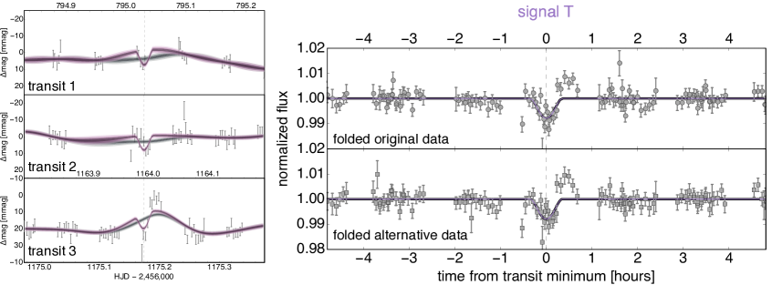
Figure 7: Same as Figure 3 except for the third transit signal found, signal T. The signal is far less convincing than than signals S and C.

Signal T immediately raises skepticism about its validity. Over 95% of the posterior trials correspond to a grazing geometry, as evident from the shape of signal T in Figure 7. As discussed earlier in Section 4.2, observational biases mean that it is 35 times more likely a detected transit would be non-grazing rather grazing. Moreover, it is generally easier for sharp data artifacts to mimic a V-shaped event than a full transit morphology, by virtue of the former’s simpler shape. The ratio-of-radii posterior is pushed up against the upper bounds of the prior, favoring a planet of $2.35_{-0.55}^{+0.48}$ $R_{\oplus}$, which is highly incompatible with the Forecaster prediction. Finally, inspection of the data itself reveals a far less convincing signal than signals C and T. We assert that signal T would never be genuinely considered a candidate transit signal of Proxima b, even if the phase had matched with the radial velocity prediction.

Because signal T would not be considered a detection if it’s phase had been compatible, we not consider is to be a false-positive signal in what follows and simply discount it from the false-positive evaluations. In contrast, signal S shows no features that would have caused us to dismiss it as a false-positive, had it landed at the correct phase. Therefore, of the 74 realizations not affected by signals C and T, 26 converge to a single spurious solution. Counting these cases as unique false-positives would imply a false-positive rate of $\mathrm{FPR}=(35\pm 7)$%, whereas counting them as belonging to a single false-positive would give $\mathrm{FPR}=(2\pm 2)$%. In conclusion, it is unclear precisely how to define the false-positive rate from these tests, but certainly the false-positive rate is non-zero and at least a few percent.

5.2 Evaluating the False-Negative (Type II) Rate

To evaluate the false-negative rate, we used the same setup as for the type I tests except we inject a 1.06 $R_{\oplus}$ planet (see Section 3.2) with $b=0.5$ into the time series at each phase point. In each of the 100 tests we ran, the model is seeking an injected Proxima b like transit signal located within the specified phase prior. Since the data has been perturbed, it was necessary to re-run the null model, $\mathcal{M}_{0}$, on each of these synthetic data sets, in addition to model $\mathcal{M}_{2}$.

We classify null detections (i.e. the false-negatives) as being any case for which criteria i & ii are not both satisfied, which occurs for 23 of our 100 simulations. This sets a minimum limit on the false-negative rate of $\mathrm{FNR}=(23\pm 5)$%.

We classify successful recoveries as cases where criteria i & ii are both satisfied and that the median of the fit’s $\tau$ posterior is less than one half of the injected transit duration from the the injected transit time. However, we exclude cases where signal C, S or T is recovered using criterion [iii] (and extended now to include signal T). Defined in this way, we count 40 successful recoveries.

In addition to 21 re-detections of signal S, 6 re-detections of signal T and 8 re-detections of signal C, we find 2 additional “detections” which do not correspond to the injected signal i.e. false-positives. We plot the credible intervals of these simulations for three key transit parameters in Figure 8, where we color code each of these cases.

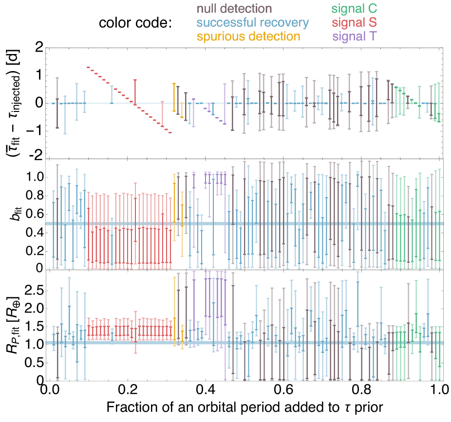
Figure 8: 1 (dark bars) and 2 (light bars) $\sigma$ credible intervals from 100 model $\mathcal{M}_{2}$ fits on the original MOST data with a Proxima-b-like transit injected at different phases ($x$-axis). Color coded key is at the top. The horizontal bars on each plot denote the value of the injected signal.

Ignoring the previous re-detections, leaves 65 simulations, of which 2 are false-positives and 40 are successful recoveries. First, this supports the previous argument for a false-positive rate of a few percent (here $(3\pm 3)$%). Second, it implies that the false-negative rate may be as high as $\mathrm{FNR}=(39\pm 8)$%.

5.3 Summary

Since we lack a complete model to describe the noise structure of our data, new synthetic, representative data sets cannot be generated to evaluate the false-positive and negative rate of our putative Proxima b transit (signal C). This limits our options to using the original data itself, which is unfortunately contaminated by three signals - the putative signal itself and two additional, likely spurious, signals.

Although these signals severely impede our ability to investigate the error rates of signal C, we estimate that the false-positive rate is at least a few percent, whereas the false-negative rate is considerably higher at $\sim 20$-$40\%$. Both of these numbers are sufficiently high to warrant serious skepticism regarding the reality of signal C.

At this point, we concluded that the MOST data alone were unable to conclusively confirm or reject this candidate signal. Whilst MOST data has some unique challenges due to the orbital motion and data sparsity, we consider that the most likely reason why this analysis is so challenging is not associated with MOST itself but rather with Proxima’s high flare activity, which leads to likelihood mis-specification.

Cross-validation is perhaps the model selection tool least likely to suffer from the affects of likelihood mis-specification. As mentioned earlier, this is impractical with just two transits observed by MOST for signal C. However, cross-validating the signal against other data sets would be a viable and robust way to establish the reality of signal C. Accordingly, we discuss such a test in the next section.

6 CROSS-VALIDATING WITH HATSouth DATA

6.1 Observations

Independent of the MOST observations, Proxima Cen was also monitored by the HATSouth ground-based telescope network (Bakos et al., 2013). The network consists of six wide-field photometric instruments located at three observatories in the Southern hemisphere (Las Campanas Observatory (LCO) in Chile, the High Energy Stereoscopic System (HESS) site in Namibia, and Siding Spring Observatory (SSO) in Australia) with two instruments per site. Each instrument consists of four 18 cm diameter astrographs and associated 4K$\times$4K backside-illuminated CCD cameras and Sloan $r$-band filters, placed on a common robotic mount. The four astrographs and cameras together cover a $8.2^{\circ}\times 8.2^{\circ}$ mosaic field of view at a pixel scale of $3\farcs 7$ pixel^-1.

Observations of a field containing Proxima Cen were collected as part of the general HATSouth transit survey, with a total of 11071 composite $3\times 80$ s exposures gathered between 2012 June 14 and 2014 September 20. These include 3430 observations made with the HS-2 unit at LCO, 4630 observations made with the HS-4 unit at the HESS site, and 3011 observations made with the HS-6 unit at the SSO site. Due to weather, and other factors, the cadence was non uniform. The median time difference between consecutive observations in the full time series is 368 s.

The data were reduced to trend-filtered light curves using the aperture photometry pipeline described by Penev et al. (2013) and making use of the External Parameter Decorrelation (EPD) procedure described by Bakos et al. (2010) and the Trend Filtering Algorithm (TFA) due to Kovács et al. (2005). One notable change with respect to the procedure described by Penev et al. (2013) is that we made use of the proper-motion-corrected positions of celestial sources from the UCAC4 catalog (Zacharias et al., 2013) to determine the astrometric solution for each image and to position the photometric apertures. This modification was essential for Proxima Cen which, at the start of the HATSouth observations, was displaced by 48″ (13 pixels) from its J2000.0 location, and moved a total of $8\farcs 7$ (2.4 pixels) over the 828 days spanned by the observations. In this paper we use these data solely to cross-validate the candidate transit signals seen in the MOST light curve. The stellar variability of Proxima Cen as revealed by HATSouth, and a general search for transits in its light curve, will be discussed elsewhere. The EPS and TFA processed data are made available in Table 5.

Table 5: Reduced HATSouth photometry used in this work, after correction for systematic trends by TFA. A portion of the table is shown here, the full version is available in the electronic version of the paper and at this URL.

HJDUTC - 2,451,545	TFA Magnitude	Uncertainty
4547.6443629	7.17666	0.0018
4547.6501446	7.18168	0.0018
4595.5309943	7.22295	0.0016
4598.5210661	7.20900	0.0017
4598.5250688	7.22170	0.0014
4598.5290578	7.23077	0.0014
4598.5333811	7.22926	0.0015
4598.5360740	7.23682	0.0027
⋮	⋮	⋮

We passed the TFA light curve through a median filter to remove 4 $\sigma$ outliers and the final photometric light curve contains 10869 data points spanning 206 nights (see Figure 9). We find that the formal measurement uncertainties greatly underestimate the observed scatter with $\sqrt{\chi^{2}/n}=7.3$ and thus, in what follows, we treat these uncertainties as relative weights but not as reliable estimates of the uncertainty on each point.

We note that the light curve of Proxima Cen shows higher scatter at short time scales than most stars observed by HATSouth in the same field with comparable brightness. Stars within $0.1$ mag of Proxima Cen have a median post-TFA r.m.s. at the same cadence of 5.3 mmag. For comparison Proxima Cen has an r.m.s. of 13.4 mmag without the additional 4 sigma clipping and median filtering, or 10.1 mmag after these additional cleaning procedures are applied. This high scatter is likely astrophysical in nature, and may be attributable to rapid low-amplitude variations in brightness due to magnetic activity such as flaring.

Figure 9: TFA-corrected photometric observations of Proxima with HATSouth from three observing seasons shown at native 240 s cadence (gray bars) and nightly averages (circles). The TFA procedure suppresses real low-frequency variability in addition to removing instrumental trends. The variation seen at $HJD-2456850$ is the residual, after TFA, of a much larger 79 mmag low-frequency astrophysical variation caused by the rotation of star spots.

6.2 Detrending

In order to look for the signal C transit, the TFA light curve requires detrending. We initially attempted to use a Gaussian process, as was used for the MOST data and experimentation with different kernels again favored the Matérn-3/2 with a characteristic covariance time scale of $s=5.6\pm 0.4$ hours.

Unlike with the analysis of the MOST data though, we are not attempting to conduct a joint fit of a GP+transit model but rather simply wish to detrend the light curve using a GP-only model. This difference is important because GPs are highly flexible and as a detrending tool can actually remove the signals we seek.

In our case, we wish to fold the detrended data upon signal C’s ephemeris and look for coherent signal. The GP, particularly with a covariance time scale of just a few hours, is sufficiently flexible to detrend both the long-term changes and potential transits themselves. Indeed, we can verify this is true since we initially attempted to perform the cross-validation using the GP detrended curves but were unable to recover any injected signals in 100 attempts.

Instead, we used a more tried and tested method for HATSouth data: median filtering. Based on previous experience with HATSouth data, a 2 day window was selected. By injecting fake transits into the HATSouth data and applying the median filtering, we found that 2 days did not remove the injected events. In contrast, when we set the median filtering time scale to 6-12 hours, we observed many injected signals were not recovered. For these reasons, we ultimately settled on the 2 day window.

6.3 Cross-validation

Phase-folding the detrended HATSouth light curve on the maximum a-posteriori ephemeris of signal C reveals visually evident disagreement between the expected model and the observations, as shown in Figure 10. Note that the phase-folded light curve modifies the limb darkening coefficients to account for the fact HATSouth is nearly a Sloan r’ bandpass (we used the nearest $T_{\mathrm{eff}}$-$\log g$ grid entry from the tabulated list of limb darkening coefficients in Claret (2004) for the PHOENIX stellar atmosphere results).

We binned the phase-folded light curve of 10869 points to 6-point bins in phase and computed the weighted mean and weighted standard deviation on each bin. This process enables us to compute realistic uncertainties on each binned point, to overcome the fact the formal uncertainties on the unbinned data are underestimates. Against a simple flat line model though, the 1806 binned points have a $\chi^{2}=2966$, indicating these weighted standard deviation still somewhat underestimate the true uncertainty. Accordingly, we scale them up by a factor of 1.645 such that $\chi^{2}=n$.

The $\chi^{2}$ of the maximum a-posteriori solution of model $\mathcal{M}_{2}$ should be lower than a simple flat line, if the transit were real, but instead it is slightly higher at $\chi_{\mathcal{M}2}^{2}-\chi_{0}^{2}=8.4$ for 1803 binned points. As a likelihood ratio, this corresponds to a 2.4 $\sigma$ preference for the null model. Repeating for $\mathcal{M}_{3}$ reveals a similar situation, with $\chi_{\mathcal{M}3}^{2}-\chi_{0}^{2}=4.4$, or a 1.6 $\sigma$ preference for the null model. The slight dip seen around the time of transit minimum i Figure 10 can be understood as due to autocorrelation, which detect a very significant $p$-value for in the phase-folded data.

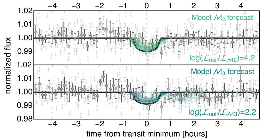
Figure 10: Phase-folded light curve of the detrended HATSouth data on the maximum a-posteriori ephemeris from model $\mathcal{M}_{2}$ (upper) and $\mathcal{M}_{3}$ (lower), corresponding to signal C. The HATSouth data does not favor a model with signal C included.

However, this single realization does not capture the range of plausible models allowed by models $\mathcal{M}_{2}$ & $\mathcal{M}_{3}$. To assess this, we took each posterior sample, performed a phase fold and re-binning of the unbinned data, and then calculated the $\chi^{2}$ of each model draw relative to the phase-binned HATSouth data. At each trial, we re-normalized the errors such that a flat line through the data yielded a $\chi^{2}$ equal to the number of data points, in order to fairly reproduce the procedure described earlier. The resulting distributions in $\Delta\log\mathcal{L}=-\Delta\chi^{2}/2$ for models $\mathcal{M}_{2}$ and $\mathcal{M}_{3}$ are shown in Figure 11.

Figure 11 reveals that signal C is clearly not confirmed by this cross-validation exercise. Indeed, for both $\mathcal{M}_{2}$ and $\mathcal{M}_{3}$, the majority of the draws favor a null model over the transit model (73% of samples for $\mathcal{M}_{2}$; 70% of samples for $\mathcal{M}_{3}$).

To provide some context, we injected 100 signal C-like transits into the HATSouth at equally spaced phases and found greater $\Delta\log\mathcal{L}$ values than those observed even in the tail of signal C’s predictions.

Figure 11: Histogram of the likelihood ratio between a null model and the phase-folded transit of signal C conditioned on the HATSouth data using the posterior samples from models $\mathcal{M}_{2}$ (light green) and $\mathcal{M}_{3}$ (dark green). The gray smoothed histogram shows the distribution from 100 injections of a signal-C-like planet phase-folded upon the injected ephemeris.

We conclude that the HATSouth data do not provide compelling supporting evidence for the existence of signal C and moderately disfavor it’s existence at the 1-2 $\sigma$ level. Excluding the signal to greater confidence will likely require far-red, near-infrared, or infrared photometry, such as that which could be provided by MEarth or Spitzer. Given the sizable false-positive/negative rate of the MOST data, the high rate and amplitude of flares produced by Proxima, the a-priori low transit probability (1.5%) and the lack of support from independent ground-based photometry, we conclude that there is not a compelling case to be made that our best candidate signal for a transit of Proxima b is genuine.

7 DISCUSSION & CONCLUSIONS

In this work, we have searched for the transits of the recently announced planetary candidate, Proxima b (Anglada-Escudé et al., 2016), in two seasons (2014 & 2015) of space-based photometry obtained using the MOST satellite. Proxima b has an a-priori transit probability of 1.5%, an expected depth of 5 mmag lasting up to an hour (Anglada-Escudé et al., 2016). Accordingly, the signal, should it exist, was expected to be quite detectable with our photometry, which after detrending exhibits an RMS of 2-3 mmag per minute with over 15,000 photometric points spanning 43.5 days at a duty cycle of $\sim 30$%.

Proxima Centauri exhibits a few percent level photometric variability in the MOST bandpass and displays dozens of detectable flares (Davenport et al., 2016). After removing obvious flares detected with the FBEYE approach (Davenport et al., 2014), we still expect a much greater number of smaller flares to exist in our data. Indeed, Davenport et al. (2016) predict 5 mmag flares (the expected transit depth of Proxima b) to occur every 20 minutes, on average. The sheer volume of such large flare events greatly complicates our analysis and we argue in this work that even our preferred model for the time correlated variability, a Gaussian process (GP) with a Matérn-3/2 kernel, is unlikely to be an accurate description of the star’s true behavior.

We conduct Bayesian model selection of a GP-only versus GP+transit model using the multimodal nested sampling algorithm MultiNest (Feroz & Hobson, 2008; Feroz et al., 2009). However, the mis-specified likelihood function formally invalidates the Bayes factors which result. Nevertheless, if we assume that the sign of the Bayes factor is correct and impose an informative prior on the period and transit mid-time based of the radial velocity fits of Anglada-Escudé et al. (2016), then we do find a candidate transit signal for Proxima b in our data, which we label as signal C.

Signal C’s freely fitted planetary radius is consistent with that expected based on the empirical, probabilistic mass-radius relation of Chen & Kipping (2016) using the Forecaster package, at $1.23_{-0.15}^{+0.13}$ $R_{\oplus}$. As expected, repeating the fits but imposing an extra informative prior on the radius using Forecaster recovers the same signal. However, when we relax the transit mid-time (or phase) informative prior, a stronger transit signal is detected at a phase incompatible (at 4 $\sigma$) with that expected from the radial velocities, which we label as signal S.

Since our noise model is argued to be inaccurate, we are unable to generate synthetic data sets for false-positive/negative tests. Instead, we use the original data and perturb the original fit’s phase prior 100 times and repeat the fit. These tests reveal a false-positive rate of at least a few percent and a much higher false-negative rate of 20-40%. This process is complicated by the presence of signal C and S in the data set though, as well an additional signal detected during these tests dubbed signal T, which is likely spurious based on it’s V-shaped morphology.

To resolve the validity of signal C, we phase-folded HATSouth photometry onto the best-fitted ephemeris of our model and a flat-line provides a slightly preferred description at 1-2 $\sigma$ significance. Repeating for the posterior draws of our model fit reveals that $\sim 75$% of our model predictions give a worse likelihood than a simple flat-line model through the HATSouth data. This final test leads to conclude our signal C is unlikely to be associated with Proxima b and is most likely a spurious detection driven by the time correlated noise structure of our data. As a result of the high false-positive and -negative rates, even when the period of the signal is known, we did not pursue a blind-period search on this data set, since the reliability of any “detections” would be highly doubtful.

The high flare activity of Proxima Centauri poses a serious challenge for any photometric follow-up of Proxima b. Even if Proxima b is detected to transit, we predict that precise transmission spectroscopy of its atmosphere would be impacted by the flares. The most promising avenue to photometrically follow-up Proxima will likely be in the red end of the visible spectrum, or with infrared measurements, where the star will not only be brighter ($K=4.4$ versus $V=11.1$) but the influence of hot flares should be attenuated. Indeed, far-red/near-infrared/infrared follow-up of the candidate transit signal reported here is recommended to conclusively exclude its existence.

References

- Anglada-Escudé et al. (2016) Anglada-Escudé, G., Amado, P., Barnes, J., et al. 2016, Nature, 536, 437
- Bakos et al. (2010) Bakos, G. Á., Torres, G., Pál, A., et al. 2010, ApJ, 710, 1724
- Bakos et al. (2013) Bakos, G. Á., Csubry, Z., Penev, K., et al. 2013, PASP, 125, 154
- Batalha et al. (2013) Batalha, N. M., Rowe, J. F., Bryson, S. T., et al. 2013, ApJS, 204, 24
- Benedict et al. (1998) Benedict, G. F., McArthur, B., Nelan, E., et al. 1998, AJ, 116, 429
- Berta-Thompson et al. (2015) Berta-Thompson, Z. K., Irwin, J., Charbonneau, D., et al. 2015, Nature, 527, 204
- Bessell (1991) Bessell, M. S. 1991, AJ, 101, 662
- Chen & Kipping (2016) Chen, J., & Kipping, D. M. 2016, ArXiv e-prints, arXiv:1603.08614
- Christian et al. (2004) Christian, D. J., Mathioudakis, M., Bloomfield, D. S., Dupuis, J., & Keenan, F. P. 2004, ApJ, 612, 1140
- Claret (2004) Claret, A. 2004, A&A, 428, 1001
- Claret et al. (2014) Claret, A., Dragomir, D., & Matthews, J. M. 2014, A&A, 567, A3
- Davenport et al. (2016) Davenport, J. R. A., Kipping, D. M., Sasselov, D., Matthews, J. M., & Cameron, C. 2016, ArXiv e-prints, arXiv:1608.06672
- Davenport et al. (2014) Davenport, J. R. A., Hawley, S. L., Hebb, L., et al. 2014, ApJ, 797, 122
- Demory et al. (2009) Demory, B.-O., Ségransan, D., Forveille, T., et al. 2009, A&A, 505, 205
- Dragomir et al. (2013) Dragomir, D., Matthews, J. M., Eastman, J. D., et al. 2013, ApJ, 772, L2
- Dressing & Charbonneau (2015) Dressing, C. D., & Charbonneau, D. 2015, ApJ, 807, 45
- Endl & Kürster (2008) Endl, M., & Kürster, M. 2008, A&A, 488, 1149
- Evans et al. (2015) Evans, T. M., Aigrain, S., Gibson, N., et al. 2015, MNRAS, 451, 680
- Feng et al. (2016) Feng, F., Tuomi, M., Jones, H. R. A., Butler, R. P., & Vogt, S. 2016, MNRAS, 461, 2440
- Feroz & Hobson (2008) Feroz, F., & Hobson, M. P. 2008, MNRAS, 384, 449
- Feroz et al. (2009) Feroz, F., Hobson, M. P., & Bridges, M. 2009, MNRAS, 398, 1601
- Gibson et al. (2012) Gibson, N. P., Aigrain, S., Roberts, S., et al. 2012, MNRAS, 419, 2683
- Jao et al. (2014) Jao, W.-C., Henry, T. J., Subasavage, J. P., et al. 2014, AJ, 147, 21
- Kipping (2011) Kipping, D. M. 2011, PhD thesis, PhD Thesis, 2011
- Kipping & Sandford (2016) Kipping, D. M., & Sandford, E. 2016, ArXiv e-prints, arXiv:1603.05662
- Kovács et al. (2005) Kovács, G., Bakos, G., & Noyes, R. W. 2005, MNRAS, 356, 557
- Mandel & Agol (2002) Mandel, K., & Agol, E. 2002, ApJ, 580, L171
- Muirhead et al. (2012) Muirhead, P. S., Johnson, J. A., Apps, K., et al. 2012, ApJ, 747, 144
- Penev et al. (2013) Penev, K., Bakos, G. Á., Bayliss, D., et al. 2013, AJ, 145, 5
- Rowe et al. (2006) Rowe, J. F., Matthews, J. M., Kuschnig, R., et al. 2006, Mem. Soc. Astron. Italiana, 77, 282
- Tuomi et al. (2014) Tuomi, M., Jones, H. R. A., Barnes, J. R., Anglada-Escudé, G., & Jenkins, J. S. 2014, MNRAS, 441, 1545
- van Leeuwen (2007) van Leeuwen, F. 2007, A&A, 474, 653
- Vanderburg et al. (2015) Vanderburg, A., Montet, B. T., Johnson, J. A., et al. 2015, ApJ, 800, 59
- Walker et al. (2003) Walker, G., Matthews, J., Kuschnig, R., et al. 2003, PASP, 115, 1023
- Winn et al. (2011) Winn, J. N., Matthews, J. M., Dawson, R. I., et al. 2011, ApJ, 737, L18
- Zacharias et al. (2013) Zacharias, N., Finch, C. T., Girard, T. M., et al. 2013, AJ, 145, 44
- Zechmeister et al. (2009) Zechmeister, M., Kürster, M., & Endl, M. 2009, A&A, 505, 859