H.E.S.S. observations of RX J1713.7$-$3946 with improved angular and spectral resolution: Evidence for gamma-ray emission extending beyond the X-ray emitting shell

Supernova remnants exhibit shock fronts (shells) that can accelerate charged particles up to very high energies. In the past decade, measurements of a handful of shell-type supernova remnants in very high-energy gamma rays have provided unique insights into the acceleration process. Among those objects, RX J1713.7$-$3946 (also known as G347.3$-$0.5) has the largest surface brightness, allowing us in the past to perform the most comprehensive study of morphology and spatially resolved spectra of any such very high-energy gamma-ray source. Here we present extensive new H.E.S.S. measurements of RX J1713.7$-$3946, almost doubling the observation time compared to our previous publication. Combined with new improved analysis tools, the previous sensitivity is more than doubled. The H.E.S.S. angular resolution of $0.048^{\circ}$ ($0.036^{\circ}$ above 2 TeV) is unprecedented in gamma-ray astronomy and probes physical scales of 0.8 (0.6) parsec at the remnant’s location.

The new H.E.S.S. image of RX J1713.7$-$3946 allows us to reveal clear morphological differences between X-rays and gamma rays. In particular, for the outer edge of the brightest shell region, we find the first ever indication for particles in the process of leaving the acceleration shock region. By studying the broadband energy spectrum, we furthermore extract properties of the parent particle populations, providing new input to the discussion of the leptonic or hadronic nature of the gamma-ray emission mechanism.

1 Introduction

Highly energetic particles with energies up to $10^{20}$ electron volts (eV, 1 eV = $1.6\times 10^{-19}$ J) hit the atmosphere of the Earth from outer space. These cosmic rays (CRs) are an important part of the energy budget of the interstellar medium. In our Galaxy the CR energy density is as large as the energy density of thermal gas or magnetic fields, yet the exact connection and interaction between these different components is poorly understood (Grenier et al. 2015).

Among the measured properties of CRs is the energy spectrum measured at Earth, which extends over many orders of magnitude. At least up to a few times $10^{15}$ eV, these particles are likely of Galactic origin – there must be objects in the Milky Way that accelerate charged particles to these energies. The composition of Galactic CRs is also known (Olive et al. 2014): at GeV to TeV energies, they are dominantly protons. Alpha particles and heavier ions make up only a small fraction of CRs. Electrons, positrons, gamma rays and neutrinos contribute less than 1%.

Establishing the Galactic sources of charged CRs is one of the main science drivers of gamma-ray astronomy. The standard paradigm is that young supernova remnants (SNRs), expanding shock waves following supernova explosions, are these accelerators of high-energy Galactic CRs (for a review, see for example Blasi 2013). Such events can sustain the energy flux needed to power Galactic CRs. In addition, there exists a theoretical model of an acceleration process at these shock fronts, known as diffusive shock acceleration (DSA) (Krymskii 1977; Axford et al. 1977; Bell 1978; Blandford & Ostriker 1978), which provides a good explanation of the multiwavelength data of young SNRs. In the past decade, a number of young SNRs have been established by gamma-ray observations as accelerators reaching particle energies up to at least a few hundred TeV. It is difficult to achieve unequivocal proof, however, that these accelerated particles are protons, which emit gamma rays via the inelastic production of neutral pions, and not electrons, which could emit very high-energy (VHE; Energies $E>100$ GeV) gamma rays via inverse Compton (IC) scattering of ambient lower energy photons. For old SNRs, for which the highest energy particles are believed to have already escaped the accelerator volume, the presence of protons has been established in at least five cases. For W28, the correlation of TeV gamma rays with nearby molecular clouds suggests the presence of protons (Aharonian et al. 2008). At lower GeV energies, four SNRs (IC 443, W44, W49B, and W51C) have recently been proven to be proton accelerators by the detection of the characteristic pion bump in the Fermi Large Area Telescope (Fermi-LAT) data (Ackermann et al. 2013; Jogler & Funk 2016; H.E.S.S. Collaboration et al. 2016c). At higher energies and for young SNRs, this unequivocal proof remains to be delivered. It can ultimately be found at gamma-ray energies exceeding about 50 TeV, where electrons suffer from the so-called Klein-Nishina suppression (see for example Aharonian (2013b) for a review), or via the detection of neutrinos from charged pion decays produced in collisions of accelerated CRs with ambient gas at or near the accelerator.

RX J1713.7$-$3946 (also known as G347.3$-$0.5) is the best-studied young gamma-ray SNR (Aharonian et al. 2004, 2006b, 2007; Abdo et al. 2011). It was discovered in the ROSAT all-sky survey (Pfeffermann & Aschenbach 1996) and has an estimated distance of 1 kpc (Fukui et al. 2003). It is a prominent and well-studied example of a class of X-ray bright and radio dim (Lazendic et al. 2004) shell-type SNRs. The X-ray emission of RX J1713.7$-$3946 is completely dominated by a non-thermal component (Koyama et al. 1997; Slane et al. 1999; Cassam-Chenaï et al. 2004; Uchiyama et al. 2003; Tanaka et al. 2008), and in fact, the first evidence for thermal X-ray line emission was reported only recently (Katsuda et al. 2015). Despite the past deep H.E.S.S. exposure and detailed spectral and morphological studies, the origin of the gamma-ray emission (leptonic, hadronic, or a mix of both) is not clearly established. All scenarios have been shown to reproduce the spectral data under certain assumptions (as discussed by Gabici & Aharonian (2014) and references therein). In addition to such broadband modelling of the emission spectra of RX J1713.7$-$3946, correlation studies of the interstellar gas with X-ray and gamma-ray emission are argued to show evidence for hadronic gamma-ray emission (Fukui et al. 2012).

We present here new, deeper, H.E.S.S. observations, analysed with our most advanced reconstruction techniques yielding additional performance improvements. After a detailed presentation of the new H.E.S.S. data analysis results and multiwavelength studies, we update the discussion about the origin of the gamma-ray emission.

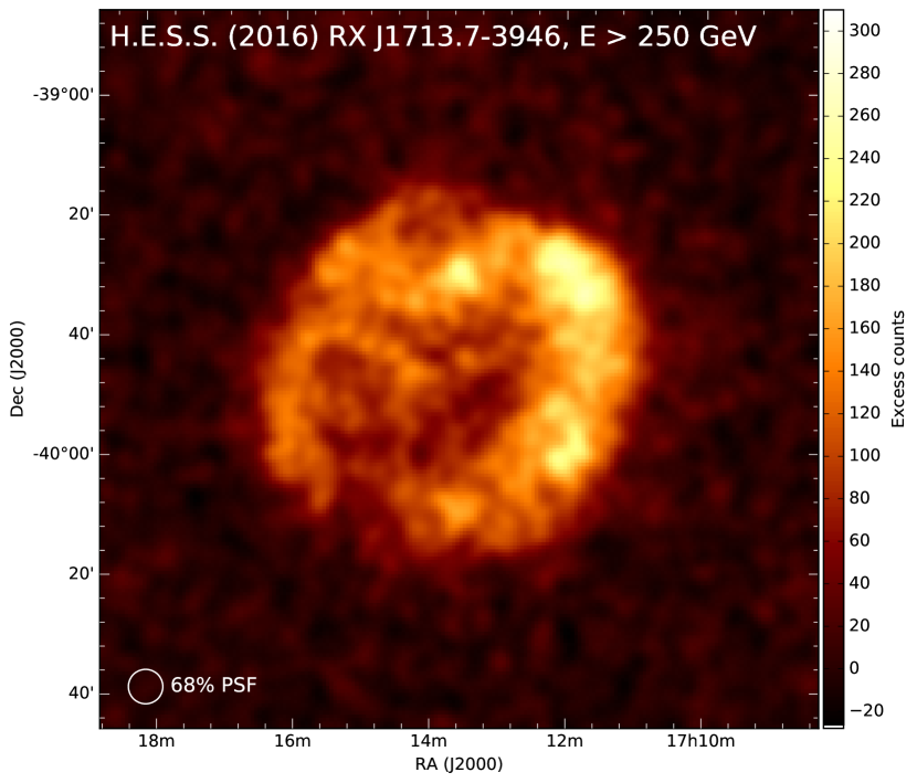
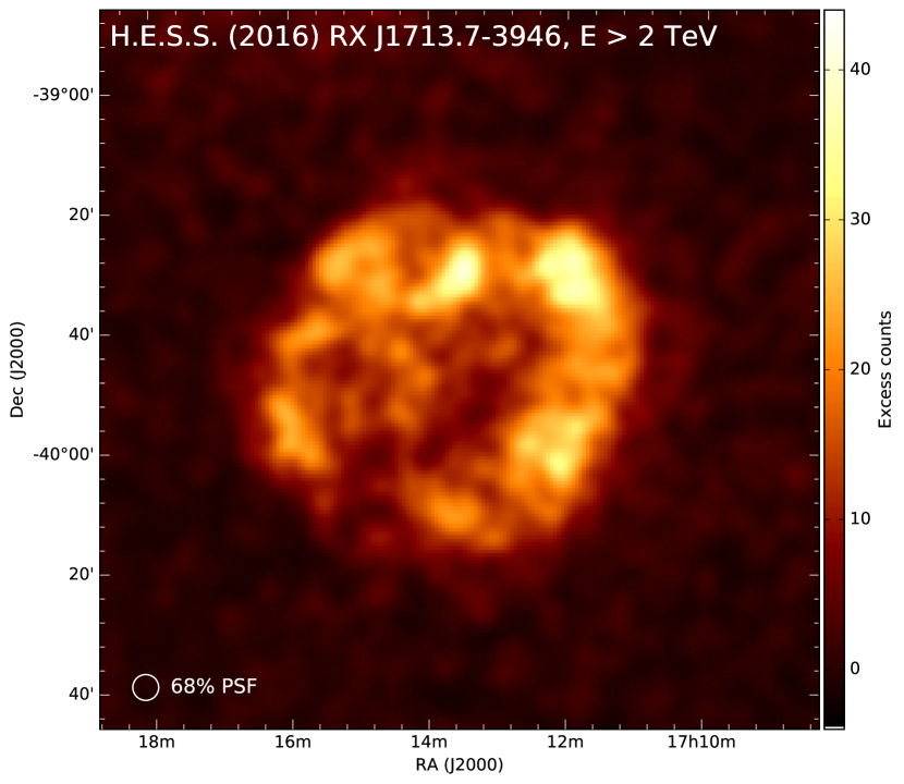
Figure 1: H.E.S.S. gamma-ray excess count images of RX J1713.7$-$3946, corrected for the reconstruction acceptance. On the left, the image is made from all events above the analysis energy threshold of 250 GeV. On the right, an additional energy requirement of $E>2$ TeV is applied to improve the angular resolution. Both images are smoothed with a two-dimensional Gaussian of width $0.03^{\circ}$, i.e. smaller than the 68% containment radius of the PSF of the two images ($0.048^{\circ}$ and $0.036^{\circ}$, respectively). The PSFs are indicated by the white circles in the bottom left corner of the images. The linear colour scale is in units of excess counts per area, integrated in a circle of radius $0.03^{\circ}$, and adapted to the width of the Gaussian function used for the image smoothing.

2 H.E.S.S. observations and analysis

The High Energy Stereoscopic System (H.E.S.S.) is an array of imaging atmospheric Cherenkov telescopes located at 1800 m altitude in the Khomas highlands of Namibia. The H.E.S.S. array is designed to detect and image the brief optical Cherenkov flash emitted from air showers, induced by the interaction of VHE gamma rays with the atmosphere of the Earth. In the first phase of H.E.S.S., during which the data used here were recorded, the array consisted of four 13 m telescopes placed on a square of 120 m side length. Gamma-ray events were recorded when at least two telescopes in the array were triggered in coincidence (Funk et al. 2004), allowing for a stereoscopic reconstruction of gamma-ray events (for further details see Aharonian et al. 2006a).

Recently H.E.S.S. has entered its second phase with the addition of a fifth, large 28 m telescope at the centre of the array. The addition of this telescope, which is able to trigger both independently and in concert with the rest of the array, increases the energy coverage of the array to lower energies. The work presented in the following sections does not use data recorded with the large telescope.

Table 1: Overview of the H.E.S.S. observation campaigns. The livetime given in hours corresponds to the data fulfilling quality requirements.

year	mean offset(1)	mean zenith angle	livetime
	(degrees)	(degrees)	(hours)
2004	0.74	30	42.7
2005	0.77	48	42.1
2011	0.73	42	65.3
2012	0.90	28	13.4

⁽¹⁾ Mean angular distance between the H.E.S.S. observation position and the nominal centre of the SNR taken to be at R.A.: 17^h13^m33.6^s, Dec.: $-$39^d45^m36^s.

The RX J1713.7$-$3946 data used here are from two distinct observation campaigns. The first took place during the years 2003–2005 and resulted in three H.E.S.S. publications (Aharonian et al. 2004, 2006b, 2007). The second campaign took place in 2011 and 2012 and is published here for the first time. In this new combined analysis of all H.E.S.S. observations the two-telescope data from 2003 (Aharonian et al. 2004) from the system commissioning phase are omitted to make the data set more homogeneous. These initial H.E.S.S. data have very limited sensitivity compared to the rest of the data set and can therefore be safely ignored. Details of the different campaigns are given in Table 1. Only observations passing data quality selection criteria are used, guaranteeing optimal atmospheric conditions and correct camera and telescope tracking behaviour. This procedure yields a total dead-time corrected exposure time of 164 hours for the source morphology studies. For the spectral studies of the SNR, a smaller data set of 116 hours is used as explained below.

The data analysis is performed with an air-shower template technique (de Naurois & Rolland 2009), which is called the primary analysis chain below. This reconstruction method is based on simulated gamma-ray image templates that are fit to the measured images to derive the gamma-ray properties. Goodness-of-fit selection criteria are applied to reject background events that are not likely to be from gamma rays. All results shown here were cross-checked using an independent calibration and data analysis chain (Ohm et al. 2009; Parsons & Hinton 2014).

3 Morphology studies

The new H.E.S.S. image of RX J1713.7$-$3946 is shown in Fig. 1: on the left, the complete data set above an energy threshold of 250 GeV (about 31,000 gamma-ray excess events from the SNR region) and, on the right, only data above energies of 2 TeV. For both images an analysis optimised for angular resolution is used (the hires analysis in de Naurois & Rolland 2009) for the reconstruction of the gamma-ray directions, placing tighter constraints on the quality of the reconstructed event geometry at the expense of gamma-ray efficiency. This increased energy requirement ($E>2$ TeV) leads to a superior angular resolution of $0.036^{\circ}$ ($68\%$ containment radius of the point-spread function; PSF) compared to $0.048^{\circ}$ for the complete data set with $E>250$ GeV. These PSF radii are obtained from simulations of the H.E.S.S. PSF for this data set, where the PSF is broadened by 20% to account for systematic differences found in comparisons of simulations with data for extragalactic point-like sources such as PKS 2155–304 (Abramowski et al. 2010). This broadening is carried out by smoothing the PSF with a Gaussian such that the $68\%$ containment radius increases by 20%. To investigate the morphology of the SNR, a gamma-ray excess image is produced employing the ring background model (Berge et al. 2007), excluding all known gamma-ray emitting source regions found in the latest H.E.S.S. Galactic Plane Survey catalogue (H.E.S.S. Collaboration et al. 2016b) from the background ring.

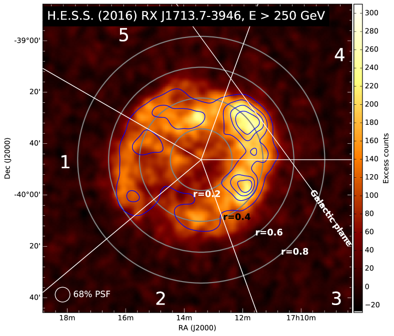
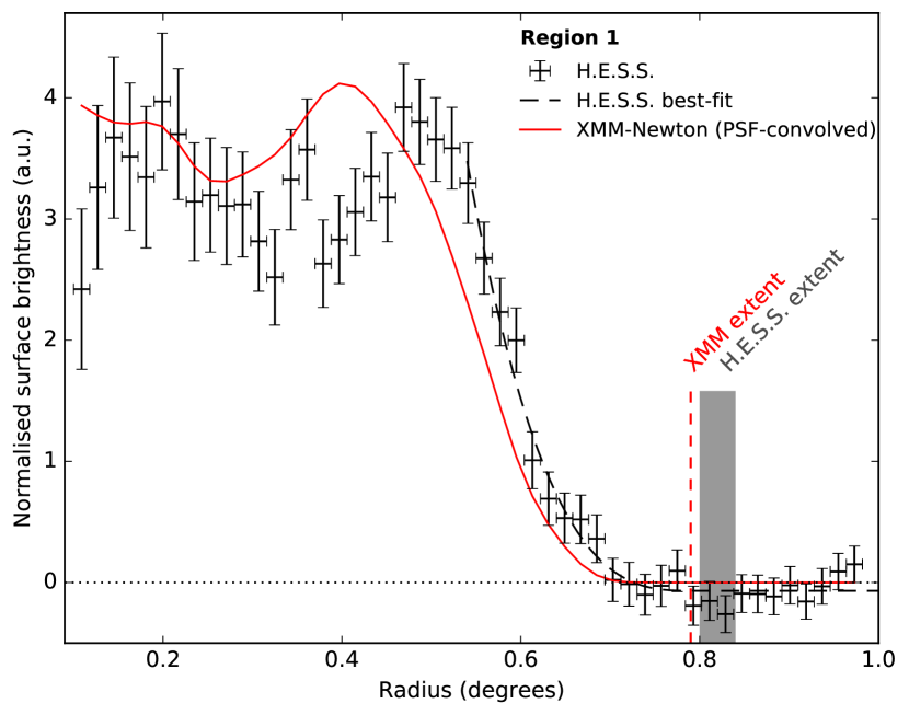
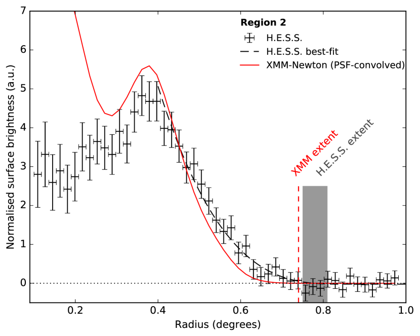
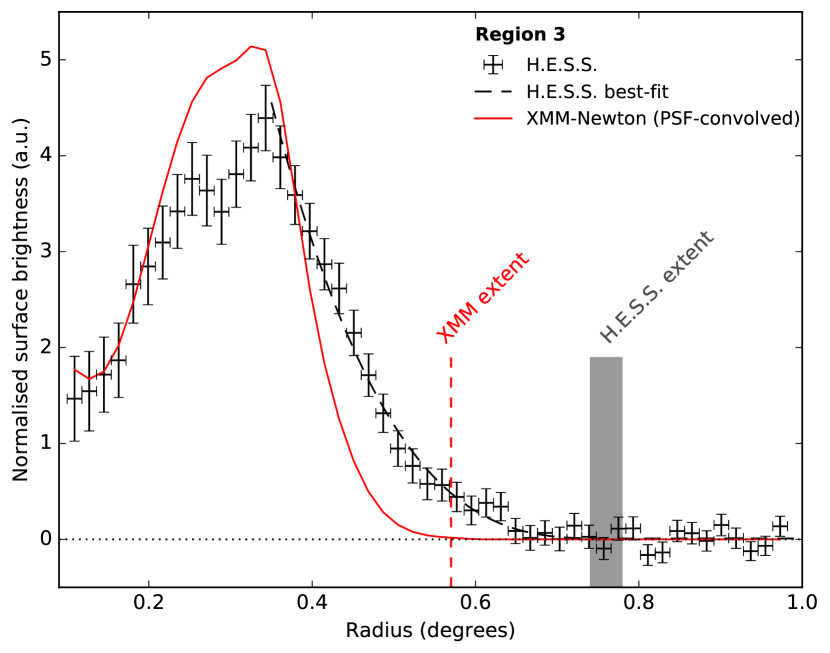
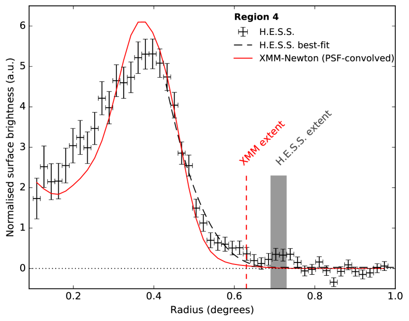
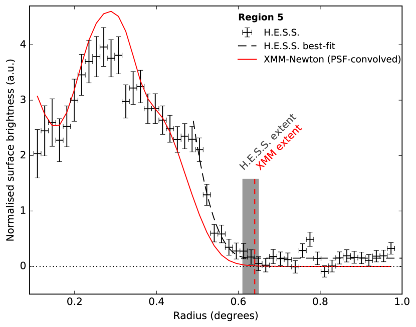
Figure 2: Gamma-ray excess map and radial profiles. Top left: the H.E.S.S. gamma-ray count map ($E>250$ GeV) is shown with XMM-Newton X-ray contours (1–10 keV, smoothed with the H.E.S.S. PSF) overlaid. The five regions used to compare the gamma-ray and X-ray data are indicated along with concentric circles (dashed grey lines) with radii of $0.2^{\circ}$ to $0.8^{\circ}$ and centred at R.A.: 17^h13^m25.2^s, Dec.: $-$39^d46^m15.6^s. The Galactic plane is also drawn. The other five panels show the radial profiles from these regions. The profiles are extracted from the H.E.S.S. maps (black crosses) and from an XMM-Newton map convolved with the H.E.S.S. PSF (red line). The relative normalisation between the H.E.S.S. and XMM-Newton profiles is chosen such that for regions 1, 2, 4 the integral in $[0.3^{\circ},0.7^{\circ}]$ is the same, for regions 3, 5 in $[0.2^{\circ},0.7^{\circ}]$. The grey shaded area shows the combined statistical and systematic uncertainty band of the radial gamma-ray extension, determined as described in the main text. The vertical dashed red line is the radial X-ray extension. For the X-ray data, the statistical uncertainties are well below 1% and are not shown.

The overall good correlation between the gamma-ray and X-ray image of RX J1713.7$-$3946, which was previously found by H.E.S.S. (Aharonian et al. 2006b), is again clearly visible in Fig. 2 (top left) from the hard X-ray contours (XMM-Newton data, 1–10 keV, described further below) overlaid on the H.E.S.S. gamma-ray excess image. For a quantitative comparison that also allows us to determine the radial extent of the SNR shell both in gamma rays and X-rays, radial profiles are extracted from five regions across the SNR as indicated in the top left plot in Fig. 2. To determine the optimum central position for such profiles, a three-dimensional spherical shell model, matched to the morphology of RX J1713.7$-$3946, is fit to the H.E.S.S. image. This toy model of a thick shell fits five parameters to the data as follows: the normalisation, the $x$ and $y$ coordinates of the centre, and the inner and outer radius of the thick shell. The resulting centre point is R.A.: 17^h13^m25.2^s, Dec.: $-$39^d46^m15.6^s. As seen from the figure, regions 1 and 2 cover the fainter parts of RX J1713.7$-$3946, while regions 3 and 4 contain the brightest parts of the SNR shell, closer to the Galactic plane, including the prominent X-ray hotspots and the densest molecular clouds (Maxted et al. 2013; Fukui et al. 2012). Region 5 covers the direction along the Galactic plane to the north of RX J1713.7$-$3946.

3.1 Production of radial profiles

The H.E.S.S. radial profiles shown in Fig. 2 are extracted from the gamma-ray excess image. To produce the X-ray radial profiles, the following procedure is applied. One mosaic image is produced from all available archival XMM-Newton data following the method described by Acero et al. (2009). All detected point-like sources are then removed from the map, refilling the resulting holes using the count statistics from annular regions surrounding the excluded regions. The cosmic-ray-induced and instrumental backgrounds are subtracted from each observation using closed filter wheel data sets. To subtract the diffuse Galactic astrophysical background from the XMM-Newton map, the level of the surface brightness at large distances ($>0.7^{\circ}$) from the SNR centre, well beyond the SNR shell position, is used. Through comparison with the ROSAT all-sky survey map (Snowden et al. 1997), which covers a much larger area around RX J1713.7$-$3946, it is confirmed that the baseline Galactic diffuse X-ray flux level is indeed reached within the field of view of the XMM-Newton coverage of RX J1713.7$-$3946 (see Fig. 12 in the appendix). An energy range of 1–10 keV is chosen for the XMM-Newton image to compare to the H.E.S.S. data to suppress Galactic diffuse emission at low energies $<1$ keV as much as possible while retaining good data statistics.

To compare the X-ray profiles to the H.E.S.S. measurement, the background is first subtracted from the XMM-Newton mosaic. In a second step, the X-ray map is then convolved with the H.E.S.S. PSF for this data set to account for the sizeable difference in angular resolution of the two instruments. The resulting radial X-ray profiles are shown in red in Fig. 2. The relative normalisation of the H.E.S.S. and XMM-Newton profiles, chosen such that the integral from 0.3^∘ to 0.7^∘ is identical for regions 1, 2, and 4 and 0.2^∘ to 0.7^∘ for regions 3 and 5, is arbitrary and not relevant for the following comparison of the radial shapes, where only relative shape differences are discussed.

3.2 Comparisons of the gamma-ray and X-ray radial profiles

A number of significant differences between X-rays and gamma rays appear in the radial profiles in all five regions. In region 1, the supposed gamma-ray shell appears as a peak around $0.5^{\circ}$ distance from the SNR centre whereas it is at $0.4^{\circ}$ in X-rays. In region 2, pronounced differences appear below $0.3^{\circ}$. The central X-ray emission in this region is brighter than the rather dim X-ray shell, which is a behaviour that is not present in the gamma-ray data. In region 3, the X-ray shell peak between $0.3^{\circ}$ and $0.4^{\circ}$ is relatively brighter and stands out above the gamma-ray peak, as was already noted by Tanaka et al. (2008) (see their Fig. 18 and related discussion) and later by Acero et al. (2009). The X-ray peak is also falling off more quickly: the decline between the peak position and a radius of $0.7^{\circ}$ is significantly different. The gamma-ray data are entirely above the X-ray data between $0.4^{\circ}$ and $0.7^{\circ}$. Regions 4 and 5 show similar behaviour; for instance, in region 3 the X-ray peak is above the gamma-ray peak, but the X-ray data fall off more quickly at radii beyond the peak. The gamma-ray data are then above the X-ray data for radii $\gtrsim 0.5^{\circ}$.

3.3 Determination of the SNR shell extent

	H.E.S.S.				XMM-Newton
Region	Fit range	$c$	$r_{0}$	$\delta r_{1/e}$	Fit range	$r_{0}$	$\delta r_{1/e}$
	(degrees)	(10-2 counts / pixel)	(degrees)	(degrees)	(degrees)	(degrees)	(degrees)
1	0.54–1.0	$-$3.4 $\pm$ 1.9${}_{\mathrm{stat}}\,\pm$ 2.0sys	0.82 $\pm$ 0.02stat	$-$	0.54–1.0	0.79	$-$
2	0.40–1.0	$-$1.1 $\pm$ 1.9${}_{\mathrm{stat}}\,\pm$ 2.0sys	0.78 $\pm$ 0.03stat	0.14 $\pm$ 0.02stat	0.42–1.0	0.74	0.10
3	0.35–1.0	0.6 $\pm$ 1.8${}_{\mathrm{stat}}\,\pm$ 3.0sys	0.76 $\pm$ 0.02stat	0.11 $\pm$ 0.01stat	0.35–1.0	0.57	0.06
4	0.43–1.0	2.2 $\pm$ 1.8${}_{\mathrm{stat}}\,\pm$ 2.0sys	0.71 $\pm$ 0.02stat	0.07 $\pm$ 0.01stat	0.43–1.0	0.63	0.06
5	0.49–1.0	9.9 $\pm$ 1.6${}_{\mathrm{stat}}\,\pm$ 3.0sys	0.63 $\pm$ 0.02stat	$-$	0.49–1.0	0.64	$-$

Table 2: Results from the radial extension measurement. The quoted errors indicate statistical uncertainties from the fit and systematic uncertainties from background normalisation.

Besides the general notion that the hotspots in X-rays are relatively brighter than those in VHE gamma rays, the profiles in all regions seem to suggest that the radial extension of the gamma-ray data exceeds that of the X-ray data: gamma rays are measured from regions beyond the X-ray shell. To quantify this effect, an algorithm was developed to measure the radial extent of the SNR emission in both data sets. For this purpose, the simple differentiable function $P(r)$,

$$P(r)=\left\{\begin{array}[]{ll}A\times\left|r_{0}-r\right|^{n}+c&\mathrm{for}\leavevmode\nobreak\ r\leq r_{0}\\ c&\mathrm{for}\leavevmode\nobreak\ r>r_{0}\end{array}\right.\mathrm{,}$$ (1)

is fit to the radial profiles.

Here, $r$ is the distance from the centre, $r_{0}$ is the parameter determining the radial size of the emission region, $A$ is a normalisation factor and $c$ is a constant to account for eventual flat residual surface brightness in the map. The exponent is fixed empirically at a value of $n=3$ in all fits and a systematic bias due to this choice is not found (see below). The fit ranges are chosen such that the start always coincides with the beginning of the falling edge of the profiles. We verified that the exact choice of the starting value of the fit has no impact on the results as long as it is beyond the peak or the rising part of the profile. Validation plots demonstrating the excellent match of the best-fit model with the gamma-ray profiles are shown in the appendix (see Fig. 8).

Table 2 lists the best-fit results with statistical uncertainties. In regions 1–4, the constant $c$ is compatible with zero within errors, showing that no large-scale flat excess emission beyond the SNR shell is seen towards these regions. The parameter $c$ is significantly positive only for region 5, hinting at a diffuse gamma-ray excess flux along the Galactic plane in this region.

The systematic uncertainty of the absolute normalisation of the ring background map is at the 1–2% level (see Berge et al. 2007). To investigate its influence on the best-fit parameters, the background normalisation is varied by $\pm$ 2% before subtraction from the raw event map and the fit is repeated. The only parameter that shows a change at a comparable level to the statistical uncertainties is the constant $c$, whereas $r_{0}$ remains largely unaffected. The resulting systematic uncertainty is at a negligible level of $0.002^{\circ}$. This demonstrates that the free parameter $c$ helps to mitigate the effects of systematic background uncertainties on the value of $r_{0}$. The parameter offsets due to background normalisation are quoted as systematic uncertainties in Table 2. The choice of the exponent $n$ has a systematic effect on the results, such that higher values of $n$ lead to higher values of $r_{0}$. To avoid biassing the gamma-ray to X-ray comparison of the $r_{0}$ values, the exponent is fixed at $n=3$ for both the H.E.S.S. and XMM-Newton fits. The exact choice of $n$ influences the absolute values of $r_{0}$ in both wavelength regimes to a similar degree without affecting the relative difference. The combined statistical and systematic uncertainty for the H.E.S.S. data is indicated in the radial profiles in Fig. 2 as a grey shaded band.

A fit with the same function (Eq. 1) is performed to determine the radial extent of the X-ray profiles from the PSF-convolved XMM-Newton map. Similar to the H.E.S.S. profiles, the model describes the data very well (see appendix, Fig. 8) and the fit results for $r_{0}$ are listed in Table 2. Statistical uncertainties are not given in this case because the fit is performed on profiles from an oversampled PSF-convolved map. The statistical quality of the XMM-Newton data is in any case very high such that the uncertainties (well below 1%) are negligible compared to those of H.E.S.S.

The two dominant sources of systematic effects when measuring $r_{0}$ in the XMM-Newton data are uncertainties in the true angular resolution of H.E.S.S. (relevant for the PSF smearing), and the estimation of the level of the Galactic diffuse background in the X-ray map. The first issue is addressed using a conservative H.E.S.S. PSF model that is broadened to cover systematic uncertainties. The latter issue is again taken into account by the constant $c$ in the fit function (Eq. 1) that compensates for flat homogeneous offsets in the map.

An additional parameter, $\delta r_{1/e}$, is listed in Table 2 for regions 2, 3, and 4. This parameter is defined as the radial distance between the peak shell emission, which is assumed to be the position of the shock, and the position where the peak emission has dropped to $1/e$ of its value. This parameter is used because it is robust against systematic uncertainties of the PSF tails and because it is often used as a measure of the diffusion length scale of particles (see below). The difference of this parameter $\delta r_{1/e}$ between X-rays and gamma rays is used in Sect. 6.2 below in the discussion of the radial differences in terms of particle diffusion. For regions 1 and 5, the shock position in X-rays in the raw un-smoothed map is not clearly defined. We are therefore only quoting $\delta r_{1/e}$ values for regions 2, 3, and 4.

In all regions we also tested for differences in the extent of the gamma-ray and X-ray profiles in energy bands, splitting up the data into $E<1$ TeV, $1<E<3$ TeV, $E>3$ TeV. There is no additional significant energy dependent difference visible in the data: the H.E.S.S. data behaviour is identical in the entire energy range covered. We also verified that this energy independence persists when using larger radii of the ring background model ($1.1^{\circ}$) to make sure that the standard ring radius ($0.8^{\circ}$) does not cancel any energy dependence.

In the appendix, we also present an independent approach to measure the extension of the SNR shell using a border-detection algorithm (see Sect. C). The same conclusions are reached with this algorithm: the gamma-ray emission extends beyond the X-ray emission. We also note that the procedure described above when performed on H.E.S.S. maps extracted from two subsets of the data of roughly equal exposure (years 2004/2005 and 2011/2012) shows no significant variation of the best-fit parameters of more than 2 $\sigma$ between the two independent data sets.

3.4 Summary of the morphology studies: Emission beyond the X-ray shell

Figure 2 demonstrates very clearly that there are significant differences between the X-ray and gamma-ray data of RX J1713.7$-$3946. While some of the differences within the bright western shell region were seen before (Tanaka et al. 2008; Acero et al. 2009), we find for the first time significant differences between X-rays and gamma rays in the radial extent of the emission associated with the SNR RX J1713.7$-$3946. These differences do not depend on energy; we find the same behaviour for $E<1$ TeV, $1<E<3$ TeV, and $E>3$ TeV. As seen from Table 2, the TeV gamma-ray emission extends significantly beyond the X-ray emission associated with the SNR shell in region 3, and there is also similarly strong evidence in region 4. We see the same tendency in regions 1, 2, and 5, although the algorithm we chose to measure the radial extent does not result in a significant radial extension difference in these regions. The border-finder algorithm, on the other hand, yields a larger TeV gamma-ray extension of the entire SNR (see appendix C).

We interpret these findings as gamma rays from VHE particles that are in the process of leaving the main shock region. The main shock position and extent are visible in the X-ray data, as discussed below in Sect. 6.2, the gamma-ray emission extending further is either due to accelerated particles escaping the acceleration shock region or particles accelerated in the shock precursor region. This is a major new result as it is the first such finding for any SNR shell ever measured.

4 Energy spectrum studies

The gamma-ray energy spectrum of RX J1713.7$-$3946 is investigated here in two different ways: we first present the new H.E.S.S. spectrum of the whole SNR region, and second we present an update of the spatially resolved spectral studies of the SNR region.

4.1 Spectrum of the full remnant

The large H.E.S.S. data set available for a spectral analysis of RX J1713.7$-$3946 comprises observation positions that vary over the years because the data are from both dedicated pointed campaigns of RX J1713.7$-$3946 and the H.E.S.S. Galactic plane survey (H.E.S.S. Collaboration et al. 2016b). When applying the standard H.E.S.S. spectral analysis, only 23 hours of observations are retained because in the standard procedure the cosmic-ray background in the gamma-ray source region (the ON region) of radius $0.6^{\circ}$ is modelled with the reflected-region background model (Berge et al. 2007). In this approach, a region of the same size and shape as the ON region (the so-called OFF region) is reflected about the centre of the array field of view and all events reconstructed in the OFF region constitute the cosmic-ray background to be subtracted from the ON region. However, for the RX J1713.7$-$3946 data set and sky field, close to the Galactic plane with other gamma-ray sources nearby, many observation runs in which OFF regions overlap partly with known gamma-ray sources are excluded from the analysis. These 23 hours of exposure resulting from the standard H.E.S.S. procedure are even below the exposure of our previous publication (Aharonian et al. 2007) because we exclude more nearby gamma-ray source regions from the prospective OFF regions. These new excluded gamma-ray sources were unknown at the time that we performed the previous analysis of RX J1713.7$-$3946. The dramatic exposure loss (23 hours remaining from an initial 164 hours of observation time) is therefore calling for a new, modified approach.

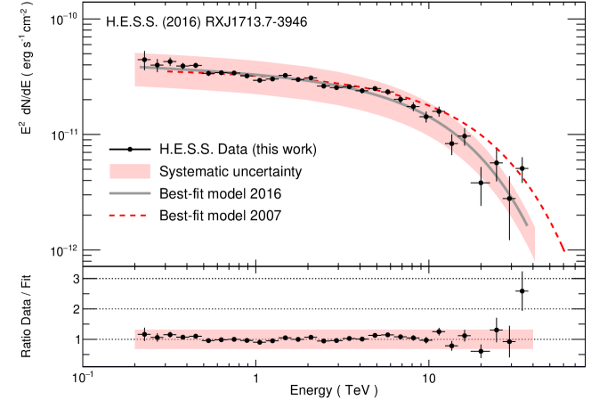
Figure 3: H.E.S.S. energy flux spectrum. Upper panel: the black data points with statistical 1 $\sigma$ error bars are the energy spectrum of the full SNR RX J1713.7$-$3946, using an extraction radius of 0.6^∘ centred on R.A.: 17^h13^m33.6^s, Dec.: $-$39^d45^m36^s. The binning is chosen to match the energy resolution, requiring a minimum significance of 2 $\sigma$ per bin. The grey solid line shows the best-fit exponential cut-off power-law model, (2) from Table 3. The dashed red line shows the corresponding best-fit model from the previous H.E.S.S. publication (Aharonian et al. 2007). The experimental flux systematic uncertainty of $\pm 32\%$, described further in the main text, is indicated as a light red band. Lower panel: the residuals are shown including statistical and systematic uncertainties.

Table 3: Results of the spectral fitting procedure on the full remnant analysis for a number of spectral models. The fits are performed using a finely binned SNR energy spectrum, whereas the spectrum shown in Fig. 3 has coarser binning for presentation purposes.

Spectral Model	$\Gamma$	$E_{\mathrm{cut}}$	$F(>1$ TeV)	$F_{0}$, at 1 TeV	$\chi^{2}$ / ndf
		(TeV)	(10-11 cm-2 s-1)	(10-11 cm-2 s-1 TeV-1)
(1) : $F_{0}E^{-\Gamma}$	2.32 $\pm$ 0.02	-	1.52 $\pm$ 0.02	2.02 $\pm$ 0.08	304 / 118
(2) : $F_{0}E^{-\Gamma}\exp\left(-(E/E_{\mathrm{cut}})^{1}\right)$	2.06 $\pm$ 0.02	12.9 $\pm$ 1.1	1.64 $\pm$ 0.02	2.3 $\pm$ 0.1	120 / 117
(3) : $F_{0}E^{-\Gamma}\exp\left(-(E/E_{\mathrm{cut}})^{2}\right)$	2.17 $\pm$ 0.02	16.5 $\pm$ 1.1	1.63 $\pm$ 0.02	2.08 $\pm$ 0.09	114 / 117
(4) : $F_{0}E^{-\Gamma}\exp\left(-(E/E_{\mathrm{cut}})^{1/2}\right)$	1.82 $\pm$ 0.04	2.7 $\pm$ 0.4	1.63 $\pm$ 0.02	4.0 $\pm$ 0.2	142 / 117

For this purpose, we employed the reflected-region technique on smaller subregions of the SNR. The circular ON region of 0.6^∘ radius, centred on R.A.: 17^h13^m33.6^s, Dec.: $-$39^d45^m36^s as in Aharonian et al. (2006b, 2007), is split into 18 subregions each of similar size. The exposures of these regions vary between 97 and 130 hours. For each of the subregions, the ON and OFF energy spectra are extracted using the reflected-region-background model, and then they are combined yielding the spectrum of the full SNR with improved exposure and statistics.

During the combination procedure, we need to account for partially overlapping OFF background regions. This is carried out by correcting the statistical uncertainties for OFF events that are used multiple times in the background model (60% of the events). Moreover, the exposure is not homogeneous across the subregions, which may lead to biasing effects towards more exposed regions in the combined spectrum. To deal with this issue, the spectrum of the whole SNR is determined as the exposure-weighted sum of all subregion spectra, rescaled to the average exposure of the SNR before merging, and conserving the original statistical uncertainties through error propagation. The resulting spectrum of the full SNR is shown in Fig. 3, and the energy flux points are listed in appendix F. This spectrum corresponds to a livetime of 116 hours, an improvement of more than a factor of two over our previous publications. This final energy spectrum and in particular the split-ON-region spectral analysis has been cross-checked with an independent analysis using the reflected-pixel background technique, as described in Abramowski et al. (2011). This cross-check yields a comparable gain in livetime and provides consistent results.

The new spectrum shown here is fit with a power-law model without and with exponential cut-off. A best-fit model with a cut-off at 12.9 TeV is preferred at 13.5 $\sigma$ over a pure power-law model as can be seen from Table 3. The cut-off models are also fit as super and sub-exponential versions (models (3) and (4) in the table) motivated by Kelner et al. (2006) who have derived analytical expressions for the gamma-ray spectra from inelastic proton-proton interactions, and these expressions suggest such exponential cut-offs at varying degrees. While the sub-exponential cut-off, model (4), is statistically disfavoured, both the super-exponential model (3) and the simple exponential cut-off model (2) describe the data well. The latter is used below and in Fig. 3 as a baseline model to describe our data.

Owing to the high statistical quality of the spectrum, the statistical errors of the best-fit spectral parameters are smaller than the systematic uncertainties discussed below. Taking both types of uncertainties into account, these new results are compatible with our previous spectrum (Aharonian et al. 2007) except for a moderate discrepancy at the highest energies. The systematic tendency of all new flux points above about 7 TeV to lie below the previous fit seen in Fig. 3 was traced down to the optical efficiency correction procedure in the old analysis (Aharonian et al. 2007). The procedure is now improved and avoids a bias above 10 TeV.

This experimental systematic uncertainty on the absolute reconstructed flux is $\pm 32\%$ for the analysis and data set used here. This uncertainty is conservatively determined as the quadratic sum of the H.E.S.S. flux uncertainty of $\pm 20\%$ for a point source (Aharonian et al. 2006a) and an extended source uncertainty that is mainly due to the analysis method employed. This extended-source uncertainty is found to be $25\%$, and is determined by analysing energy spectra in 29 regions across the SNR with the primary analysis chain (de Naurois & Rolland 2009) and the cross-check chain (Ohm et al. 2009; Parsons & Hinton 2014). These are two completely different analysis approaches with independent calibration, reconstruction, analysis selection requirements, and with the same reflected-region-background model. For this purpose, both energy spectra are compared in each region by taking the difference between the best-fit models ((2) from Table 3) as measure for the systematic uncertainty at a given energy. This is carried out for all 29 regions. The resulting differences are averaged in energy bins, and the largest average deviation seen for any energy in the range covered (200 GeV to 40 TeV) is $25\%$, which is added conservatively as an additional $\pm 25\%$ systematic uncertainty to a total flux uncertainty $\Delta\,\mathrm{F}_{\mathrm{syst}}$ of

$$\Delta\,\mathrm{F}_{\mathrm{syst}}=\sqrt{(\Delta\,\mathrm{F}^{\mathrm{Crab}}_{\mathrm{syst}}=20\%)^{2}+(\Delta\,\mathrm{F}^{\mathrm{Extended}}_{\mathrm{syst}}=25\%)^{2}}=32\%\,.$$ (2)

For validation purposes, energy spectra were also extracted from two subsets of the data (years 2004/2005 and 2011/2012 separately) to test for a temporal evolution of the flux and spectral parameters of RX J1713.7$-$3946 as suggested by the model in Federici et al. (2015). We find that all spectral parameters agree within their 1 $\sigma$ uncertainty intervals during the eight years covered by the H.E.S.S. observations.

4.2 Spatially resolved spectroscopy

The unprecedented angular resolution and much improved sensitivity of H.E.S.S. has now allowed us to produce high statistics spectra of the SNR in 29 small non-overlapping boxes with $0.18^{\circ}$ or 10.8 arcminute side lengths as shown in Fig. 4 (left). These regions are identical to those chosen in Tanaka et al. (2008) for the comparison of Suzaku X-ray and H.E.S.S. gamma-ray data. For each box, the spectrum is extracted by employing the reflected-region-background model, and the resulting data are fit by a power-law model with an exponential cut-off ((2) in Table 3). The results are shown in Table 4. For some of the regions with low surface brightness we cannot derive tight constrains on the exponential cut-off energy. In these regions, a pure power-law model without a cut-off yields a similarly good fit.

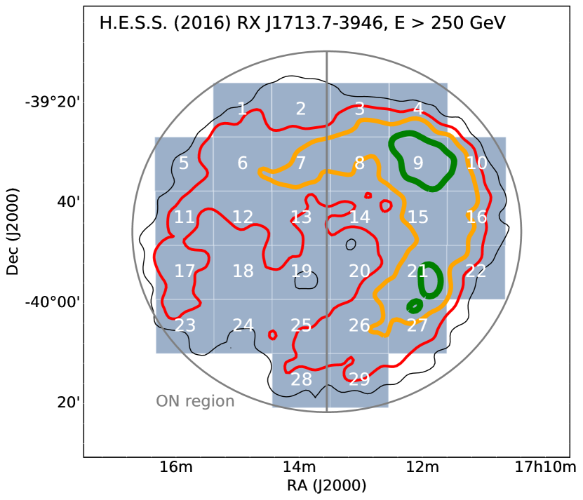
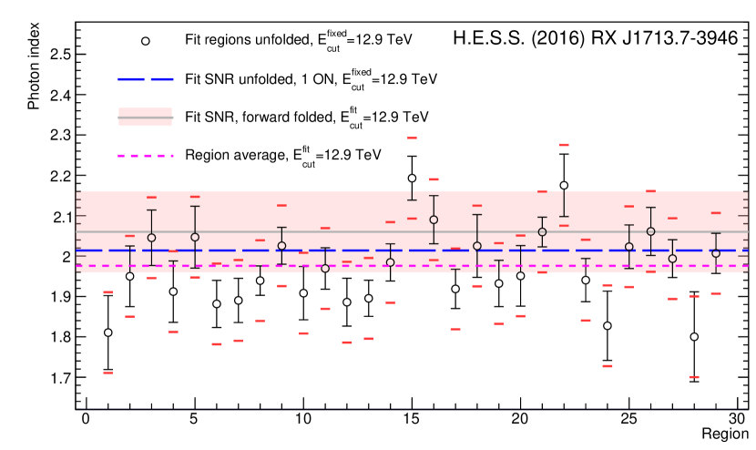
Figure 4: Results of the spatially resolved spectral analysis. On the left-hand side, the 29 regions used for this study are shown, overlaid on the H.E.S.S. gamma-ray significance contours at 3, 5, 7, and $9\,\sigma$ coloured in black, red, orange, and green. The resulting photon index distribution is shown on the right-hand side. The ON region used for the full SNR spectrum is also shown as a grey circle, the vertical grey line bisects the ON region into the western and eastern half also used for the spectral analysis. The error bars on the right-hand side are $1\,\sigma$ statistical fit uncertainties, and the additional red error intervals indicated for each point correspond to the systematic uncertainty on the reconstructed photon index of $\Delta\Gamma_{\mathrm{sys}}=0.1$, which is also shown as light red band around the forward folded SNR photon index.

Table 4: Spectral fitting results for the 29 Suzaku regions. A power law with exponential cut-off, (2) of Table 3, was fit to the gamma-ray H.E.S.S. data.

Reg.	$\Gamma$	$E_{\mathrm{cut}}$	$F(>1$ TeV)	$\chi^{2}$ / ndf
		(TeV)	(10-13 cm-2 s-1)
1	1.99 $\pm$ 0.16	20 $\pm$ 17	3.4 $\pm$ 0.6	74 / 78
2	1.95 $\pm$ 0.15	10.9 $\pm$ 6.3	4.7 $\pm$ 0.9	70 / 76
3	1.66 $\pm$ 0.22	4.2 $\pm$ 1.7	4.6 $\pm$ 1.3	58 / 77
4	1.84 $\pm$ 0.17	10.1 $\pm$ 5.5	4.1 $\pm$ 0.8	73 / 81
5	2.06 $\pm$ 0.13	25 $\pm$ 18	3.4 $\pm$ 0.5	94 / 83
6	1.72 $\pm$ 0.10	8.1 $\pm$ 2.1	8.3 $\pm$ 1.0	74 / 80
7	1.65 $\pm$ 0.11	5.8 $\pm$ 1.4	8.6 $\pm$ 1.2	97 / 79
8	1.95 $\pm$ 0.08	13.2 $\pm$ 3.9	9.6 $\pm$ 0.8	84 / 81
9	1.81 $\pm$ 0.08	7.3 $\pm$ 1.6	12.0 $\pm$ 1.1	82 / 82
10	1.90 $\pm$ 0.10	11.1 $\pm$ 3.9	6.8 $\pm$ 0.8	80 / 82
11	1.87 $\pm$ 0.11	9.8 $\pm$ 3.3	6.0 $\pm$ 0.7	119 / 80
12	1.57 $\pm$ 0.13	6.0 $\pm$ 1.5	6.6 $\pm$ 1.2	79 / 81
13	1.69 $\pm$ 0.12	7.0 $\pm$ 1.9	6.8 $\pm$ 1.0	62 / 82
14	1.97 $\pm$ 0.10	12.6 $\pm$ 4.6	6.6 $\pm$ 0.7	67 / 83
15	1.99 $\pm$ 0.09	8.4 $\pm$ 2.5	8.4 $\pm$ 0.9	89 / 77
16	2.02 $\pm$ 0.09	14.7 $\pm$ 5.4	7.6 $\pm$ 0.7	88 / 81
17	1.80 $\pm$ 0.11	9.3 $\pm$ 2.8	6.4 $\pm$ 0.8	76 / 80
18	1.34 $\pm$ 0.22	2.8 $\pm$ 0.8	5.1 $\pm$ 1.5	83 / 80
19	1.82 $\pm$ 0.12	10.3 $\pm$ 4.1	5.4 $\pm$ 0.8	73 / 78
20	1.77 $\pm$ 0.13	8.0 $\pm$ 2.8	5.3 $\pm$ 0.9	85 / 81
21	1.98 $\pm$ 0.09	9.2 $\pm$ 2.7	8.9 $\pm$ 0.9	74 / 82
22	2.14 $\pm$ 0.10	24 $\pm$ 15	5.9 $\pm$ 0.6	99 / 78
23	1.91 $\pm$ 0.12	14.0 $\pm$ 6.0	5.0 $\pm$ 0.6	81 / 80
24	1.99 $\pm$ 0.11	45 $\pm$ 42	4.0 $\pm$ 0.5	80 / 83
25	1.88 $\pm$ 0.15	6.2 $\pm$ 2.4	5.2 $\pm$ 0.9	83 / 76
26	1.76 $\pm$ 0.12	6.0 $\pm$ 1.6	7.3 $\pm$ 1.0	78 / 79
27	1.79 $\pm$ 0.09	6.2 $\pm$ 1.3	10.0 $\pm$ 1.0	84 / 81
28	1.45 $\pm$ 0.17	4.4 $\pm$ 1.2	5.5 $\pm$ 1.2	60 / 80
29	2.05 $\pm$ 0.09	17.3 $\pm$ 7.7	6.2 $\pm$ 0.6	78 / 80

The following procedure is employed to test for spatial variation of the spectral shapes measured with H.E.S.S. Each subregion is fit with a power law with an exponential cut-off, leaving the normalisation and the photon index free, but fixing the cut-off at 12.9 TeV. This is the average value obtained by fitting the energy spectrum of the whole SNR (see (2) in Table 3). We verified that the free exponential cut-off fit shown in Table 4 does not provide a statistically preferred best-fit model compared to the model with the cut-off fixed in any region. This fit procedure with a fixed cut-off allows us to directly probe all regions for a difference in the photon index $\Gamma$; fit parameter correlations between the index and the cut-off can then be ignored.

The resulting photon index comparison is shown in Fig. 4 (right). Region to region, the statistical spread around the region average is at most $3\,\sigma$. A $\chi^{2}$ test for a constant index results in a $p$ value of $0.02\%$, i.e. the index fluctuations around the region average are not compatible with statistical fluctuations alone. To evaluate whether the indices also vary significantly when taking the systematic uncertainties into account, these uncertainties on the reconstructed photon index are again determined by comparing all energy spectra, region by region, between the primary analysis chain (de Naurois & Rolland 2009) and the cross-check chain (Ohm et al. 2009; Parsons & Hinton 2014). This approach is already applied above for the systematic uncertainty of the full SNR energy spectrum. For each region, both reconstructed energy spectra are fit with a power law with the same fixed cut-off of 12.9 TeV. For all 29 regions, the resulting best-fit photon index difference distribution has an RMS spread of 0.09. This exceeds the statistical spread expected from the largely correlated data of the two independent analysis chains, and we take this value as the systematic index uncertainty. A small part of this spread may still be from statistical uncertainties, but we conservatively take the full RMS as systematic uncertainty.

Since this approach covers only the uncertainty related to the calibration and analysis method, but not, for example, the atmospheric transmission uncertainties, which are potentially as large as 0.05 (Hahn et al. 2014), we conclude that $\Delta\Gamma_{\mathrm{sys}}=0.1$ is the systematic photon index uncertainty for the H.E.S.S. data set shown here. With this, the $\chi^{2}$ test reveals a $p$ value of 57%, the photon index does therefore not vary significantly across different regions of the SNR.

As confirmation of the systematic photon index uncertainty, the energy spectrum of the whole SNR is determined in two different ways, which demonstrates how the analysis and fitting method impacts the spectral index reconstruction. For this, the energy spectrum of the primary analysis chain (see Sect. 4.1), determined by splitting the whole SNR into subregions, merging the spectra and fitting a spectral model by forward folding it with the instrument response functions, is compared to an alternative approach. For this, as described above at the expense of exposure, we use the entire SNR ON region without further splitting. We furthermore fit the flux points that were unfolded from the instrument response functions to derive the best-fit photon index. The resulting two photon index measurements of the SNR are shown in Fig. 4 (right) by the difference of $\Delta\Gamma=0.05$ of the grey solid and blue long-dashed lines, which are well contained within the quoted systematic uncertainty. The same is true for the average subregion index of 1.98 (purple short dashed line in the right panel of Fig. 4), which is compatible with the photon index of the entire SNR fit, 2.06, at the $<1\,\sigma_{\mathrm{sys}}$ level.

To conclude, there is no evidence for a spatial variation of the photon index, either from region to region or from any region to the entire SNR energy spectrum, within our statistical and systematic uncertainties.

5 Broadband modelling

The H.E.S.S. results presented above provide a new opportunity to study the origin of the VHE emission from RX J1713.7$-$3946. Even though RX J1713.7$-$3946 is one of the best-studied young SNRs with non-thermal emission, which clearly indicates the acceleration of VHE particles by the shell of the remnant, the hadronic or leptonic nature of the VHE gamma-ray emission remains a source of disagreement in the literature (Berezhko & Völk 2006; Morlino et al. 2009; Zirakashvili & Aharonian 2010; Ellison et al. 2010; Finke & Dermer 2012; Gabici & Aharonian 2014), as discussed in detail for example in Gabici & Aharonian (2016). Below, we add new information for this discussion. We use Suzaku X-ray, Fermi-LAT gamma-ray and H.E.S.S. VHE gamma-ray data to model the broadband energy spectrum of RX J1713.7$-$3946 and derive the present-age parent particle spectra from the spectral energy distribution (SED) of the SNR in both emission scenarios. We also model the broadband energy spectra, which are spatially resolved into the 29 boxes described above, using the Suzaku and H.E.S.S. data only.

Model	Parameter	Full	West	East
Hadronic	$\Gamma\mathrm{{}_{p}^{1}}$	$1.53\pm 0.09$	$1.34^{+0.18}_{-0.3}$	$1.2\pm 0.3$
	$E\mathrm{{}_{p}^{break}}$ ( TeV )	$1.4^{+0.7}_{-0.4}$	$0.78\pm 0.19$	$0.44\pm 0.12$
	$\Gamma\mathrm{{}_{p}^{2}}$	$1.94\pm 0.05$	$2.26\pm 0.03$	$2.20\pm 0.05$
	$E\mathrm{{}_{p}^{cutoff}}$ ( TeV )	$93\pm 15$	$280\pm 70$	$350^{+200}_{-100}$
	$W\mathrm{{}_{p}}$ ( $10^{49}(n_{\mathrm{H}}/1\,\mathrm{cm}^{-3})^{-1}$ erg )	$5.81\pm 0.12$	$3.93\pm 0.08$	$3.15\pm 0.09$
	AIC (broken PL)	87.0	101.5	79.3
	AIC (simple PL)	106.2	153.1	96.3
	Relative likelihood (simple vs. broken)	$7\times 10^{-5}$	0	$2\times 10^{-4}$
Leptonic (X and $\gamma$-ray)	$\Gamma\mathrm{{}_{e}^{1}}$	$1.78\pm 0.12$	$1.83\pm 0.05$	$1.92^{+0.06}_{-0.11}$
	$E\mathrm{{}_{e}^{break}}$ ( TeV )	$2.5\pm 0.3$	$2.15\pm 0.11$	$1.79^{+0.12}_{-0.2}$
	$\Gamma\mathrm{{}_{e}^{2}}$	$2.93\pm 0.02$	$3.10\pm 0.02$	$2.97\pm 0.03$
	$E\mathrm{{}_{e}^{cutoff}}$ ( TeV )	$88.4\pm 1.2$	$84.8\pm 1.5$	$120\pm 3$
	$W\mathrm{{}_{e}}$ ( $10^{46}$ erg )	$11.9\pm 0.5$	$9.0\pm 0.4$	$7.0\pm 0.4$
	$B$ ( $\mu$G )	$14.26\pm 0.16$	$16.7\pm 0.2$	$12.0\pm 0.2$
	AIC (broken PL)	116.2	157.0	112.8
	AIC (simple PL)	345.5	250.2	127.1
	Relative likelihood (simple vs. broken)	0	0	$8\times 10^{-4}$
Leptonic (only $\gamma$-ray)	$\Gamma\mathrm{{}_{e}^{1}}$	$1.6\pm 0.2$	$1.9\pm 0.3$	$2.1\pm 0.3$
	$E\mathrm{{}_{e}^{break}}$ ( TeV )	$2.0\pm 0.3$	$1.7\pm 0.3$	$1.6\pm 0.3$
	$\Gamma\mathrm{{}_{e}^{2}}$	$2.82\pm 0.04$	$3.12\pm 0.03$	$3.05\pm 0.04$
	$E\mathrm{{}_{e}^{cutoff}}$ ( TeV )	$65\pm 7$	$140\pm 30$	$210^{+13000}_{-80}$
	$W\mathrm{{}_{e}}$ ( $10^{46}$ erg )	$11.8\pm 0.5$	$10.1\pm 0.6$	$7.8\pm 0.5$
	AIC (broken PL)	80.8	104.5	83.5
	AIC (simple PL)	142.9	177.3	98.8
	Relative likelihood (simple vs. broken)	0	0	$5\times 10^{-4}$

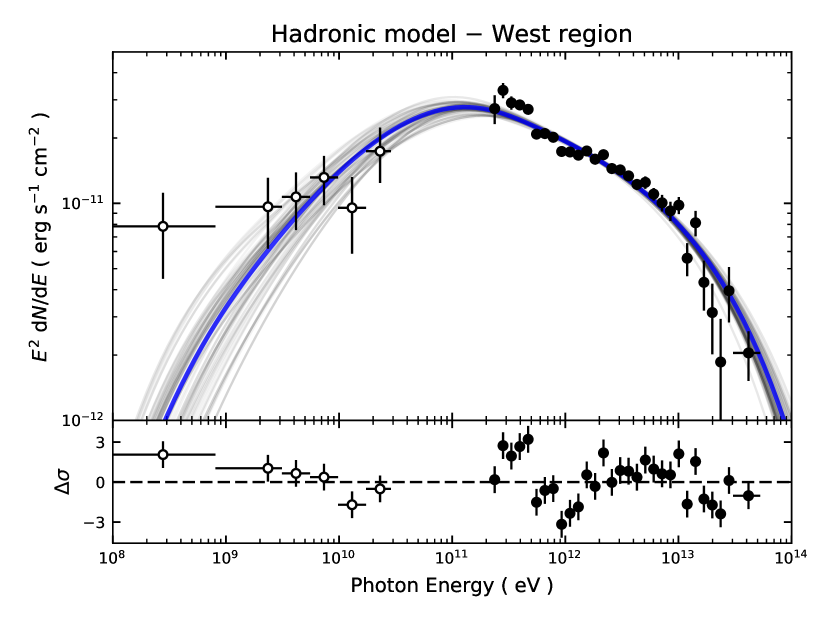
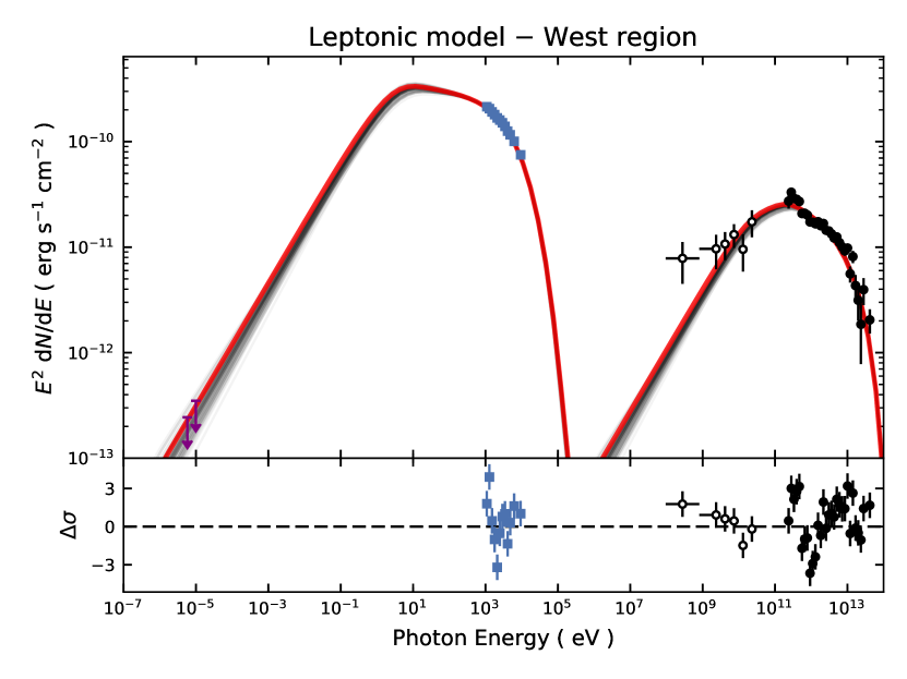
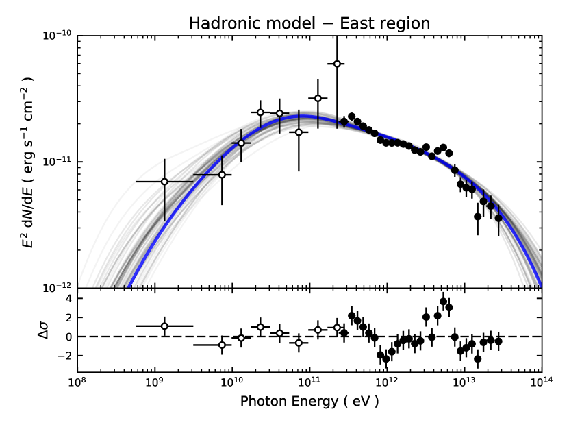
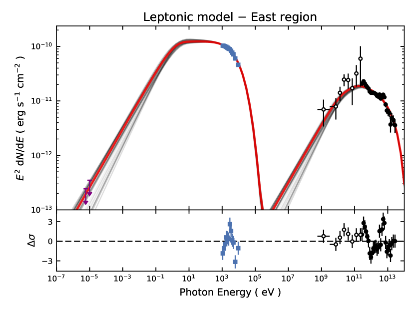
Figure 13: For the western (top) and eastern (bottom) halves of RX J1713.7$-$3946, the hadronic (left) and leptonic (right) gamma-ray models obtained by our broadband fit are shown in these figures compared to the data. The thick blue and red lines indicate the maximum-likelihood models, and the grey lines surrounding them are the models for 100 samples of the MCMC chain and serve to illustrate the fit uncertainties. The ATCA radio data (Lazendic et al. 2004) of RX J1713.7$-$3946 plotted as magenta upper limits are determined for the north-west part of the SNR shell only and are scaled up by a factor of two here and included in the fit by constraining the model to stay below these values.

Table 5: Results from the hadronic and leptonic model fits. For the leptonic model, the fit was performed to the full available broadband data from X-rays to gamma rays and restricted to the GeV to TeV gamma rays alone. The parameters are given for the full remnant, the western half, and the eastern half. To compare the fits of the simple and broken power-law models with exponential cut-off, the Akaike information criterion (AIC, Akaike 1974) is also given. The relative likelihood (see main text), set to 0 for values below $1\times 10^{-5}$, illustrates clearly that in all cases the broken power law is statistically favoured over the simple power law. The total energy in protons is given for a target density of $n_{\mathrm{H}}=1\,\mathrm{cm}^{-3}$, and both the proton and electron total energy are given above 1 TeV (for graphical versions see Figs. 5 and 13). The 1 $\sigma$ statistical errors are asymmetric, unless the difference between the up- and downward errors is less than 25%; in that case they are given as symmetric errors.

5.1 Suzaku data analysis

Tanaka et al. (2008) have presented a detailed analysis of the Suzaku data that cover most of the SNR RX J1713.7$-$3946. We performed additional Suzaku observations in 2010, adding four pointings with a total exposure time of 124 ks after the standard screening procedure, to complete the coverage of RX J1713.7$-$3946 with Suzaku. After combining the Suzaku XIS data set from Tanaka et al. (2008) with these additional pointings, we perform a spatially resolved spectral analysis for the 29 regions shown in Fig. 4 to combine the synchrotron X-ray spectrum in each region with the corresponding TeV gamma-ray spectrum in the broadband analysis below.

5.2 GeV data analysis

For the Fermi-LAT analysis, 5.2 years of data (4 August 2008 to 25 November 2013) are used. The standard event selection, employing the reprocessed P7REP_SOURCE_V15 source class, is applied to the data, using events with zenith angles less than 100^∘ and a rocking angle of less than 52^∘ to minimise the contamination from the emission from the Earth atmosphere in the Fermi-LAT field of view (Abdo et al. 2009). Standard analysis tools, available from the Fermi-LAT Science support centre, are used for the event selection and analysis. In particular, a 15^∘ radius for the region of interest and a binned analysis with 0.1^∘ pixel size is used. The P7REP diffuse model (Acero et al. 2016a) and background source list, consistent with the official third source catalogue (3FGL, Acero et al. 2015) with the addition of Source C from Abdo et al. (2011), are employed in the analysis. The binned maximum-likelihood mode of gtlike, which is part of the ScienceTools, is used to determine the intensities and spectral parameters presented in this paper. Further details of the analysis are provided in the description in Abdo et al. (2011).

For the spectral analysis, we adopt the spatial extension model based on the H.E.S.S. excess map. In the first step of the spectral analysis, we perform a maximum-likelihood fit of the spectrum of RX J1713.7$-$3946 in the energy range between 200 MeV and 300 GeV using a power-law spectral model with integral flux and spectral index as free parameters. To accurately account for correlations between close-by sources, we also allow the integral fluxes and spectral indices of the nearby background sources at less than $3^{\circ}$ from the centre of the region of interest to vary in the likelihood maximisation. In addition, the spectral parameters of identified Fermi-LAT pulsars, the normalisation and the index of an energy-dependent multiplicative correction factor of the Galactic diffuse emission model, and the normalisation of the isotropic diffuse model are left free in the fit. This accounts for localised variations in the spectrum of the diffuse emission in the fit which are not considered in the global model. For the Galactic diffuse emission, we find a normalisation factor of $1.007\pm 0.001$ in our region of interest. The normalisation factor for the remaining isotropic emission component (extra-galactic emission plus residual backgrounds not fully suppressed by the analysis requirements) is $1.17\pm 0.02$. These factors demonstrate the reasonable consistency of the local brightness and spectrum of the diffuse gamma-ray emission with the global diffuse emission model. The LAT spectrum for the emission from RX J1713.7$-$3946 is well described by a power law with $\Gamma=1.58\pm 0.06$ and an integrated flux above 1 GeV of $I=(4.1\pm 0.4)\times 10^{-9}$ cm^-2 s^-1. When fitting with different Galactic diffuse models based on alternative interstellar emission models (Acero et al. 2016b), the systematic uncertainty on the photon index is approximately 0.1 and on the normalisation above 1 GeV approximately $0.7\times 10^{-9}$ cm^-2 s^-1 (consistent with the previous study of this object, see Abdo et al. 2011).

To test for spatial differences in the emission, we split the H.E.S.S. template in an eastern and a western half: the spectrum in the west yields $\Gamma=1.74\pm 0.11$, $I=(3.1\pm 0.8)\times 10^{-9}$ cm^-2 s^-1, in the east $\Gamma=1.41\pm 0.12$, $I=(1.8\pm 0.5)\times 10^{-9}$ cm^-2 s^-1. These results show a shape agreement at the 2 $\sigma$ level when taking the statistical uncertainties into account. In addition there is a systematic error of $\Delta\Gamma_{\mathrm{syst}}^{\mathrm{Fermi}-LAT}=0.1$ from the choice of the diffuse model as tested for the overall remnant.

In a second step we perform a maximum-likelihood fit of the flux of RX J1713.7$-$3946 in 13 independent logarithmically spaced energy bands from 280 MeV to 400 GeV (using the spectral model and parameters for the background sources obtained in the previous fit) to obtain an SED for the SNR. We require a test statistic value of $TS\geq 4$ in each band to draw a data point corresponding to a $2\,\sigma$ detection significance (see Fig. 5 below).

5.3 Derivation of the present-age parent particle distribution

To understand the acceleration and emission processes that produce the observed data, the present-age particle distribution can be derived by fitting the observed energy spectra. We present below the results of the derivation of the parent particle population for both a hadronic and leptonic model for the whole remnant, for the two halves of the remnant, and for the spatially resolved spectra extracted from the 29 regions described above in Sect. 4.2. For the full and half remnant spectra, the gamma-ray spectra from Fermi-LAT and H.E.S.S. are used in the fitting, whereas only the H.E.S.S. spectra are used for the 29 spatially resolved regions because the Fermi-LAT data lacks sufficient statistics when split into these regions. For leptonic models, X-ray spectra from the Suzaku observations are also fitted simultaneously with the gamma-ray data. We used the radiative code and Markov Chain Monte Carlo (MCMC) fitting routines of naima (Zabalza 2015) to derive the present-age particle distribution, using the parametrisation of neutral pion decay by Kafexhiu et al. (2014), and of IC up-scattering of diluted blackbody radiation by Khangulyan et al. (2014). For the leptonic models, the magnetic field and exponential energy cut-off are treated as independent parameters. The magnetic field is constrained by the ratio of synchrotron to IC flux magnitude, whereas the cut-off in the parent electron spectrum is constrained by the cut-off in the VHE part of the IC gamma-ray spectrum. In the MCMC fit, the seed photon fields considered for the IC emission are the cosmic microwave background radiation and a far-infrared component with temperature $T=26.5$ K and a density of 0.415 eV cm^-3. These latter values are derived from GALPROP by Shibata et al. (2011) for a distance of 1 kpc. For hadronic gamma-ray emission, the solar CR composition is used to take the effects of heavier nuclei into account.

We note that the assumption that the emission in each of the extraction regions arises from a single particle population under homogeneous ambient conditions might not hold for several of the regions selected. In particular, whereas the IC emissivity samples the electron density, keeping in mind that the target photon field density for IC emission does not vary on small scales, the synchrotron emissivity samples the product of electron density and magnetic field energy density. Considering the inhomogeneity of magnetic field in supernova remnants, and in RX J1713.7$-$3946 in particular (Uchiyama et al. 2007), this means that the X-ray emission typically samples smaller volumes than IC emission.

5.3.1 Full remnant

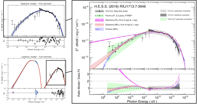
Figure 5: Comparison of hadronic and leptonic models to the data. Top left: the hadronic gamma-ray model obtained with our broadband fit is compared to data. Bottom left: the same plot of the leptonic gamma-ray model compared to data including lower-energy X-rays and radio data. The thick blue and red lines indicate the maximum-likelihood models, and the grey lines surrounding them are the models for 100 samples of the MCMC chain and serve to illustrate the fit uncertainties. The energy flux data points shown from high to low energy are the H.E.S.S. and Fermi-LAT gamma-ray data as solid and open circles, the Suzaku X-ray data and ATCA radio data (Lazendic et al. 2004). The latter flux was determined for the northwest part of the SNR shell only and was scaled up by a factor of two here to represent the whole SNR. Owing to this ad hoc scaling, these points are not included in the fit, but are shown for illustration only. Right-hand side: both leptonic and hadronic models are compared to the Fermi-LAT and H.E.S.S. data points including statistical and systematic uncertainties. In addition to the preferred best-fit models of a broken power law with a cut-off (BPL), a power law without cut-off is also shown for the leptonic model to demonstrate that this model cannot describe the Fermi-LAT gamma-ray data.

The full-remnant SED at gamma-ray energies shown in Fig. 5 exhibits a hard spectrum in the GeV regime, a flattening between $\sim$100 GeV and a few TeV, and an exponential cut-off above $\sim$10 TeV. In a hadronic scenario, this spectrum is best fit with a particle distribution consisting of a broken power law and an exponential cut-off at high energies. The results of the fit can be seen in Table 5 and Fig. 5 (top left) and Fig. 6, where the resulting best-fit gamma-ray models (left) and parent particle energy spectra (right) are shown. In Table 5, the difference between the two particle indices of the broken power law is significant, indicating a break in the proton energy distribution at an energy of $1.4\pm 0.5$ TeV. For a target density of $n_{\mathrm{H}}/1\,\mathrm{cm}^{-3}$, a total energy in protons of $W_{p}=(5.80\pm 0.12)\times 10^{49}(n_{\mathrm{H}}/1\,\mathrm{cm}^{-3})^{-1}$ erg above 1 TeV is required to explain the measured gamma-ray flux.

As in the hadronic scenario, the observed gamma-ray spectrum cannot be explained with an electron population described by a single power law. This is clearly seen on the right-hand side of Fig. 5, where the best-fit power-law electron model is shown to be incompatible with the gamma-ray data even when taking all uncertainties into account. Fitting a broken power-law electron distribution to the X-ray and gamma-ray emission from the full remnant results in a break at $E_{b}=2.4\pm 0.3$ TeV and a difference between the particle indices of $\Delta\Gamma_{e}=1.16\pm 0.14$ (see Table 5). The magnetic field strength required to reproduce the X-ray and gamma-ray spectra is $B=14.2\pm 0.2\,\mu$G.

To illustrate the need for a low-energy break in the particle energy spectrum, the Akaike information criterion (AIC; Akaike 1974) is also given in Table 5 as measure for the relative quality of both spectral models, the simple power law with exponential cut-off and the broken power law with exponential cut-off. A lower AIC value corresponds to the more likely model, the relative likelihood also given in the table is defined as $\exp{((AIC_{\mathrm{min}}-AIC_{\mathrm{max}})/2)}$. In all cases, the broken power law is clearly preferred over the simple power law. We also tested fitting a broken power law with a smooth instead of a hard transition,

$$E^{2}\,\times\,\frac{dN}{dE}\,=E^{2}\,\times\,F_{o}\,E^{-\Gamma^{1}}\,\left(1+\left(\frac{E}{E^{\mathrm{break}}}\right)^{-\frac{\Gamma^{1}-\Gamma^{2}}{\beta}}\right)^{-\beta}\,\mathrm{,}$$

plus a high-energy exponential cut-off, but find that the addition of one more parameter to our results is not justified. The hard transition, $\beta\rightarrow 0$, is mildly favoured at the $1-2\sigma$ level over a smoother transition, $\beta_{\mathrm{fit}}\approx 0.3$, for the SED of the entire SNR in both the hadronic and leptonic models. The data cannot thus discriminate between these two versions of a broken power law. We therefore use the simpler version with a hard break, which has one parameter less.

To test the impact of the X-ray data and see which fit parameters are affected more by these than the gamma-ray data, we have also performed the broadband leptonic fits only to the gamma-ray data (losing any handle on the magnetic field). The resulting parameters are shown in Table 5. Also in this case, a broken power law instead of a single power law is needed to fit the gamma-ray data, the resulting particle indices and break energy are compatible with the full broadband fit. The exponential cut-off of the parent particle spectrum, on the other hand, is significantly lower: $65\pm 7$ TeV compared to $88.4\pm 1.2$ TeV when including the X-ray data.

From the particle spectra shown in Fig. 6, one can see that electrons via IC emission are much more efficient in producing VHE gamma rays than protons via $\pi^{0}$ decay (Gabici & Aharonian 2016). A proton spectrum about 100 times higher is needed to produce nearly identical gamma-ray curves as shown in Fig. 5.

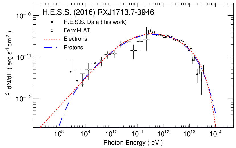
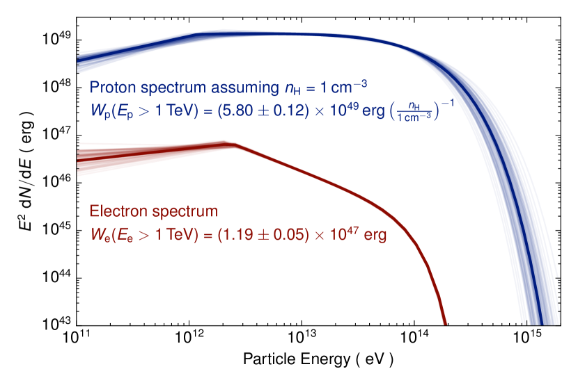
Figure 6: Gamma-ray model curves and parent particle energy spectra. On the left, the best-fit electron and proton gamma-ray models (broken power laws with exponential cut-offs) are compared to the Fermi-LAT and H.E.S.S. data. The data points and model curves are the same as in Fig. 5. On the right, the corresponding best-fit parent particle energy spectra are shown. The electron model is derived from a combined fit to both the X-ray and gamma-ray data.

5.3.2 Half remnant

Splitting the remnant ad hoc into the dim eastern and bright western halves, we can test for spatial differences in the broadband parent particle spectra within the remnant region while including the Fermi-LAT data. Using similar models to those described above, we find that for a hadronic origin of the gamma-ray emission a broken power law is statistically required to explain the GeV and TeV spectra for both halves of the remnant. The corresponding plots are shown in the appendix (Fig. 13). As can be seen in Table 5, the particle indices for the power laws from the remnant halves are compatible with the high-energy particle index of the full-remnant broken power-law spectrum, confirming that, like for the gamma-ray spectra, there is no spectral variation seen in the derived proton spectra either.

Assuming a leptonic scenario, the western half of the remnant shows a slightly stronger magnetic field strength with $B_{\mathrm{W}}=16.7\pm 0.2\,\mu$G, compared to a strength of $B_{\mathrm{E}}=12.0\pm 0.2\,\mu$G in the eastern half (Table 5). In addition, the electron high-energy cut-off measured is significantly lower in the western half, $E\mathrm{{}_{c,W}^{e}}=88.4\pm 1.2$ TeV, compared to $E\mathrm{{}_{c,E}^{e}}=120\pm 3$ TeV in the eastern half. The inverse dependency between the magnetic field strength and cut-off energy is consistent with electron acceleration limited by synchrotron losses at the highest energies. Given that the X-ray emission is produced by electrons of higher energies than the TeV emission, the energy of the exponential cut-off is constrained strongly by the X-ray spectrum. To demonstrate the impact of this, we also fit the electron spectrum only to the gamma-ray data, see Table 5. From this fit the cut-off energy increases and has much larger uncertainties. This can be explained by synchrotron losses constrained by the X-ray data. If some small regions have a magnetic field strength that is significantly higher than the average field strength, these regions can dominate the X-ray data and cause differences in the cut-off energies.

5.3.3 Spatially resolved particle distribution

The deep H.E.S.S. observations allow us to fit the broadband X-ray and VHE gamma-ray spectra from the 29 smaller subregions defined in Sect. 4.2 to probe the particle distribution and environment properties by averaging over much smaller physical regions of 1.4 pc (for a distance to the SNR of 1 kpc). However, in VHE gamma rays the resolvable scale is still much larger than some of the features observed in X-rays (Uchiyama et al. 2007). It is therefore unlikely that the regions probed here encompass a completely homogeneous environment, and information is lost due to the averaging. In addition, the projection of the near and far section of the remnant, and in fact the interior, along the line of sight into the same two-dimensional region adds an uncertainty when assessing the physical origin of the observed spectrum. This degeneracy is only broken for the rim of the remnant where the projection effects are minimal, and we know that the observed spectrum is emitted close to the shock. As before, we consider both the leptonic and hadronic scenarios for the origin of VHE gamma-ray emission.

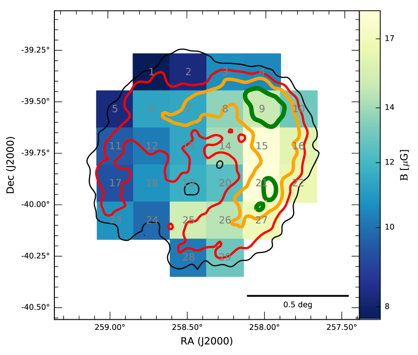
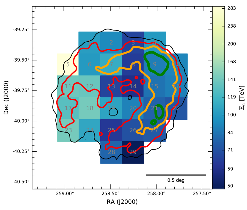
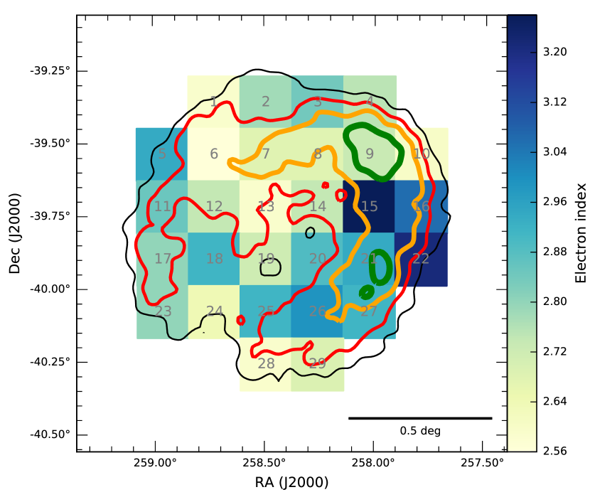
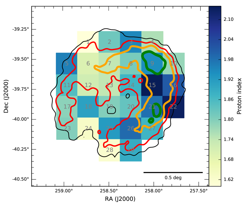
Figure 7: Spatial distribution of physical best-fit parameters across the SNR, overlaid on the H.E.S.S. gamma-ray significance contours at 3, 5, 7, and $9\,\sigma$ in black, red, orange, and green. For the leptonic model, colour codes are shown for the magnetic field strength (top left), exponential cut-off energies (top right), and particle indices (bottom left). For the hadronic models, only the particle indices (bottom right) are relevant and shown here. The 29 subregions labelled with grey numbers are boxes of side lengths $0.18^{\circ}$ or 10.8 arcminutes. To judge whether the differences region to region are significant, the statistical uncertainties listed in Table 6 and 7 have to be taken into account, and ultimately the H.E.S.S. systematic measurement uncertainties discussed above as well. When doing this, the spectral indices show no variation across the SNR in either scenario.

Reg.	Part. Index	$E_{\mathrm{c}}$	$W_{\mathrm{e}}$ ($>$1 TeV)	B
		(TeV)	($10^{45}$ erg)	($\mu$G)
1	$2.59\pm 0.18$	$102\pm 15$	$1.7^{+0.5}_{-0.4}$	$7.7\pm 0.8$
2	$2.78\pm 0.14$	$93\pm 9$	$3.4\pm 0.7$	$8.3\pm 0.7$
3	$2.84\pm 0.13$	$66^{+6}_{-5}$	$3.7\pm 0.7$	$10.6\pm 0.7$
4	$2.75\pm 0.14$	$100\pm 10$	$2.8\pm 0.6$	$10.5^{+0.9}_{-0.7}$
5	$2.94\pm 0.11$	$290^{+180}_{-70}$	$3.3\pm 0.6$	$8.3\pm 0.6$
6	$2.56\pm 0.11$	$100\pm 7$	$4.1\pm 0.6$	$11.3\pm 0.6$
7	$2.68\pm 0.09$	$112\pm 8$	$4.9\pm 0.7$	$11.4\pm 0.6$
8	$2.68\pm 0.08$	$64\pm 3$	$6.5\pm 0.7$	$13.6\pm 0.5$
9	$2.73\pm 0.06$	$87\pm 3$	$7.8\pm 0.8$	$14.9\pm 0.5$
10	$2.60\pm 0.09$	$90\pm 4$	$4.2^{+0.7}_{-0.5}$	$12.9^{+0.7}_{-0.5}$
11	$2.85\pm 0.09$	$140^{+17}_{-12}$	$4.6\pm 0.6$	$9.5\pm 0.5$
12	$2.74\pm 0.10$	$137^{+18}_{-14}$	$4.1\pm 0.6$	$10.2\pm 0.6$
13	$2.59\pm 0.09$	$66\pm 3$	$4.0\pm 0.5$	$11.4\pm 0.5$
14	$2.74\pm 0.09$	$58\pm 3$	$4.9^{+0.7}_{-0.5}$	$14.1\pm 0.6$
15	$3.26\pm 0.10$	$83^{+9}_{-7}$	$12.4\pm 1.8$	$18.2\pm 1.0$
16	$3.06\pm 0.10$	$88\pm 6$	$8.4\pm 1.2$	$16.0\pm 1.0$
17	$2.80\pm 0.08$	$129\pm 13$	$4.6\pm 0.6$	$9.3^{+0.5}_{-0.4}$
18	$2.91\pm 0.13$	$144^{+30}_{-20}$	$3.9\pm 0.8$	$10.8\pm 0.9$
19	$2.72\pm 0.10$	$106\pm 8$	$3.7\pm 0.5$	$11.7\pm 0.7$
20	$2.89\pm 0.14$	$89\pm 8$	$4.8\pm 0.9$	$12.4\pm 1.0$
21	$2.94^{+0.06}_{-0.08}$	$77\pm 4$	$8.6\pm 0.9$	$18.4\pm 0.6$
22	$3.21\pm 0.15$	$73^{+7}_{-5}$	$8.5\pm 1.7$	$16.4\pm 1.5$
23	$2.80\pm 0.09$	$144\pm 16$	$4.0\pm 0.5$	$10.8\pm 0.6$
24	$2.64\pm 0.13$	$108\pm 11$	$2.4\pm 0.5$	$9.8\pm 0.7$
25	$2.91\pm 0.10$	$62^{+4}_{-3}$	$4.8\pm 0.6$	$15.2\pm 0.8$
26	$2.99\pm 0.13$	$71\pm 4$	$8.6^{+1.7}_{-1.3}$	$14.5\pm 1.0$
27	$2.91\pm 0.09$	$75\pm 4$	$8.6\pm 1.1$	$16.7\pm 0.8$
28	$2.6\pm 0.2$	$78\pm 9$	$2.8^{+1.1}_{-0.8}$	$10.2^{+1.7}_{-1.1}$
29	$2.69\pm 0.10$	$49\pm 3$	$4.5\pm 0.6$	$12.8\pm 0.7$

Table 6: Electron distribution and magnetic field parameters derived from the VHE and X-ray spectra of the 29 regions under the assumption of an IC origin of the gamma-ray emission. The total energy in electrons $W_{e}$ is computed for electron energies above 1 TeV.

In the leptonic scenario, the Suzaku X-ray spectra are used together with the H.E.S.S. gamma-ray data in the fits. This allows us to derive the magnetic field per subregion in addition to the parameters of the electron energy distribution. Given that the Fermi-LAT GeV spectra cannot be obtained in such small regions, only electrons above $\sim$5 TeV are probed by the VHE gamma-ray and X-ray spectra, and we can only infer the properties of the high-energy part of the particle spectra, i.e. the power-law slope and its cut-off. No information about the break energy or the low-energy power law can be extracted in the subregions. In the leptonic scenario, the VHE gamma-ray emission probes the electron spatial distribution, whereas the X-ray emission probes the electron distribution times $B^{2}$, causing regions with enhanced magnetic field to be over-represented in the X-ray spectrum.

We find that in all regions the emission from an electron distribution with a power law and an exponential cut-off reproduces the spectral shape in both X-ray and VHE gamma-ray energies. Table 6 and Fig. 7 show the results of these fits. The electron particle index for all the regions is in the range 2.56 to 3.26 and is compatible with the average full-remnant particle index of 2.93. Such steep particle indices, which are significantly larger than the canonical acceleration index of about 2, indicate that the accelerated electron population at these energies ($E_{e}\gtrsim 5$ TeV) has undergone modifications, i.e. cooling through synchrotron losses. However, neither the age of the remnant of O(1000 years) nor the derived average magnetic field are high enough for the electrons to have cooled down to such energies. Explaining this spectral shape is thus a challenge for the leptonic scenario, which is discussed further in Sect. 6.1. Figure 7 (bottom left) shows that the spatial distribution of the electron index is not entirely uniform, even when taking the statistical uncertainties given in Table 6 into account the indices in the brighter western part of the shell tend to be larger. Such a trend is also seen in the distribution of the high-energy exponential cut-off energy (in the range 50–200 TeV) and the average magnetic field strength (in the range 8–20 $\mu$G) shown in the same figure. The western half of the remnant shows higher values of the magnetic field strength and lower values of the cut-off with the opposite behaviour seen in the eastern half (see top left and right of Fig. 7). In a synchrotron-loss-limited acceleration scenario, the maximum energy achievable at a given shock is proportional to $B^{-1/2}$, so that the anti-correlation between cut-off energy and magnetic field strength is to be expected.

Reg.	Part. Index	$W_{\mathrm{p}}$ ($>$1 TeV)
		($10^{48}$ erg cm-3)
1	$1.60^{+0.14}_{-0.19}$	$0.91\pm 0.09$
2	$1.82\pm 0.11$	$1.51\pm 0.11$
3	$1.95\pm 0.10$	$1.52\pm 0.12$
4	$1.76\pm 0.11$	$1.24\pm 0.10$
5	$1.96\pm 0.11$	$1.27\pm 0.10$
6	$1.70\pm 0.09$	$2.37\pm 0.17$
7	$1.74\pm 0.08$	$2.48\pm 0.15$
8	$1.81\pm 0.05$	$3.07\pm 0.13$
9	$1.94\pm 0.06$	$3.9\pm 0.2$
10	$1.78\pm 0.10$	$2.29\pm 0.15$
11	$1.85\pm 0.08$	$1.91\pm 0.11$
12	$1.72\pm 0.09$	$1.91\pm 0.13$
13	$1.74\pm 0.07$	$2.07\pm 0.11$
14	$1.87\pm 0.06$	$2.19\pm 0.11$
15	$2.14\pm 0.07$	$3.3\pm 0.2$
16	$2.01\pm 0.08$	$2.71\pm 0.19$
17	$1.79\pm 0.07$	$1.96\pm 0.11$
18	$1.91\pm 0.10$	$1.56\pm 0.14$
19	$1.80\pm 0.09$	$1.72\pm 0.10$
20	$1.83\pm 0.11$	$1.79\pm 0.15$
21	$1.98\pm 0.05$	$3.19\pm 0.15$
22	$2.13\pm 0.10$	$2.4\pm 0.2$
23	$1.80\pm 0.08$	$1.74\pm 0.10$
24	$1.63\pm 0.14$	$1.18\pm 0.09$
25	$1.92\pm 0.07$	$1.72\pm 0.11$
26	$1.99\pm 0.08$	$3.0\pm 0.2$
27	$1.87\pm 0.07$	$3.21\pm 0.19$
28	$1.62\pm 0.16$	$1.44\pm 0.19$
29	$1.89\pm 0.07$	$2.09\pm 0.12$

Table 7: Proton distribution parameters derived from the VHE gamma-ray spectra of the 29 subregions, assuming a neutral pion decay origin of the gamma-ray emission. The total energy in protons is computed for proton energies above 1 TeV. The cut-off energy is fixed to 93 TeV, which is the value obtained for the full-remnant spectrum, to overcome fit convergence problems due to limited statistics in dim regions of the SNR.

In a hadronic scenario we only consider radiation from primary protons without considering secondary X-ray emission from charged pions produced in interactions of protons with ambient matter (Aharonian 2013a). Using only the H.E.S.S. spectra, we find that the proton cut-off energy is not constrained for many of the regions. We therefore fix the cut-off energy when fitting the subregions spectrum to the value found for the full SNR spectrum: $E_{\mathrm{c}}=93$ TeV. Under this assumption, all the regions are well fit by a neutral pion decay spectrum with the parameters shown in Table 7. The proton particle indices for all the regions cover a range between 1.60 and 2.14 as shown in Fig. 7 (bottom right) and listed in Table 7. As already found above for the gamma-ray spectral fits (Sect. 4.2), the maximum difference between the particle spectral indices of different regions is at the level of 3 $\sigma$ – the indices do not vary across the SNR when taking the H.E.S.S. spectral index systematic uncertainty in addition to the statistical uncertainties given in Table 7 into account. In the hadronic scenario proposed by Gabici & Aharonian (2014) for RX J1713.7$-$3946, these particle index values are from energy spectra of protons that have completely diffused within dense small clumps of interstellar matter and are therefore altered by diffusion effects resulting in a hardening of the spectral shapes compared to the standard index of 2 expected from DSA.

6 Interpretation

6.1 Leptonic versus hadronic origin

The observational data presented in this work provide the deepest data set available to date to evaluate the physical origin of the VHE gamma-ray emission from the shell-type SNR RX J1713.7$-$3946 to find out whether the emission has a leptonic (IC upscatter of external radiation fields by relativistic electrons) or hadronic (pion decay emission from interaction of relativistic protons with ambient gas) origin. The discussion of the origin is intimately tied to the question of whether the present-age electron or proton distribution required by the observed gamma-ray spectra can be achieved considering the physical properties of the supernova remnant. Therefore, the derivation of the relativistic parent particle energy distributions presented in Sect. 5.3 is a crucial tool to evaluate theoretical scenarios for the VHE radiation of RX J1713.7$-$3946.

A notable feature in both the electron and proton energy distributions inferred in Sect. 5.3 is the spectral break at a few TeV. Gabici & Aharonian (2014), following Zirakashvili & Aharonian (2010) and Inoue et al. (2012), put forward an explanation for such a break in the hadronic scenario as the result of diffusion of protons in high-density cold clumps within the SNR: higher energy protons diffuse faster and interact with the highest density regions within the clumps, whereas lower energy protons only probe the outer, lower density regions and therefore have a lower emissivity. This scenario would arise from a massive star exploding in a molecular cloud that itself has been swept away by a wind of the progenitor star, resulting in a rarefied cavity with dense clumps. On the passage of the SNR shock, the high density ratio between the clumps and cavity effectively stalls the shock at the surface of the clumps avoiding their disruption (Inoue et al. 2012). The break energy depends on the age of the SNR and the density profile of the clouds (Gabici & Aharonian 2014). Considering a density within the clumps of $10^{3}\,\mathrm{cm}^{-3}$, the break energy is of the order of 1–5 TeV for the age of RX J1713.7$-$3946, which is consistent with the best-fit value of $E\mathrm{{}_{p}^{break}}=1.4\pm 0.5$ TeV as shown in Sect. 5.3.1. This scenario would explain the very low level of thermal X-ray emission recently reported (Katsuda et al. 2015), and it is also consistent with the average density of $130\,\mathrm{cm}^{-3}$ integrated over the SNR and the cavity walls reported in Fukui et al. (2012). In this cold clump scenario, the proton energetics given in Table 5 for $n=1\,\mathrm{cm}^{-3}$ would only correspond to the protons interacting within these clumps of $n=10^{3}\,\mathrm{cm}^{-3}$. To obtain the total energy in protons, a filling factor correction based on the combined clumps and SNR shell volume ratio ($V_{\mathrm{clumps}}/V_{\mathrm{shell}}$) is needed.

In the leptonic scenario, a break in the electron spectrum could arise due to synchrotron losses: electrons at higher energies suffer faster synchrotron cooling and therefore a break is introduced at the energy for which the synchrotron loss timescale and SNR age are equal,

$$E_{b}\simeq 1.25\left(\frac{B}{100\,\mu\mathrm{G}}\right)^{-2}\left(\frac{t_{0}}{10^{3}\,\mathrm{yr}}\right)^{-1}\ \mathrm{TeV.}$$ (3)

Considering an SNR age of the order of 1000 yr, a magnetic field of $\sim$70 $\mu$G would be required for a cooling break at 2.5 TeV, the best-fit value found in Sect. 5.3.1. While there are indeed indications for such high magnetic fields from X-ray variability measurements of small filaments (Uchiyama et al. 2007), or the X-ray width of the filaments itself (see for example Vink 2012, and references therein), the residence time of electrons in these small regions is much shorter than the age of the SNR and thus too short for significant synchrotron cooling. The best probe we have of the relevant magnetic field strength that may explain such a cooling break, averaged over a volume large enough so that the electron residence time is sufficiently long, is the simultaneous fitting of X-ray and gamma-ray data of the whole SNR presented here. The results in Sect. 5.3.1 indicate a present-age average magnetic field strength of $B=14.3\pm 0.2\,\mu$G for the SNR, which is much less than the 70 $\mu$G required to explain the energy break according to Eq. 3. This remains a challenge in the leptonic scenario. In particular, experimental systematic uncertainties are also unable to explain this energy break, as clearly shown in Fig. 5 (right).

Two alternative explanations of the flattening between 10 GeV and a few TeV of the SED of RX J1713.7$-$3946 are discussed in the literature. Firstly, a second population of VHE electrons is suggested for example by Finke & Dermer (2012). With different electron populations the relevant physical parameters may be tuned in a way that would exactly reproduce the flat spectral shape of RX J1713.7$-$3946. Alternatively, a single power-law electron population in the presence of an additional optical seed photon field, as discussed in Tanaka et al. (2008), could produce the broad measured shape. We argue that this explanation is unlikely since such a photon field would require an unrealistically large energy density of $\sim$140 eV cm^-3, which is more than two orders of magnitude above the standard estimates, for example implemented in GALPROP (Porter et al. 2006) at the position of the remnant. Beyond such simplified models, approaches taking the temporal and spatial SNR evolution into account have also been shown to reproduce the GeV to TeV gamma-ray data in a leptonic scenario (see for example Ellison et al. 2012).

6.2 Particles beyond the shock

The X-ray synchrotron emission from RX J1713.7$-$3946 is expected to be mostly confined to the region within the shock front. Very high-energy electrons must also be present beyond the shock, but the magnetic field in the unshocked medium is a factor $\mathcal{R}_{\mathrm{B}}\approx 3$ (see for example Parizot et al. 2006) smaller than in the shocked medium. $\mathcal{R}_{\mathrm{B}}$ is the magnetic field compression ratio. It depends on the magnetic field orientation and is generally comparable but smaller than the shock compression ratio $\mathcal{R}$, which is $\mathcal{R}=4$ for a strong shock. Since the synchrotron emissivity scales with $B^{\Gamma}$ (Ginzburg & Syrovatskii 1965), where $\Gamma\approx 2$ (Acero et al. 2009) is typically the synchrotron X-ray photon index here, the X-ray synchrotron emissivity is expected to drop by a factor $\mathcal{R}_{\mathrm{B}}^{\Gamma}=9$ at the shock. The boundary of the X-ray emission therefore traces the shock front of RX J1713.7$-$3946. The evidence presented in Sect. 3.3 for gamma-ray emission outside the X-ray boundary requires the presence of accelerated particles beyond the shock front.

Since the electrons outside the shock experience the same radiation energy density as those within the shock boundary, the emissivity does not sharply drop at the shock in the case that the leptonic emission scenario (IC scattering) applies to the VHE gamma-ray emission of RX J1713.7$-$3946. For standard hadronic emission scenarios, the emissivity should change at the shock boundary as the density of the ambient medium increases across the shock and drops again beyond it. But this standard hadronic scenario is not relevant for RX J1713.7$-$3946 since it fails to explain the hard gamma-ray emission in the GeV band. The alternative scenario mentioned in Sect. 6.1 requires the presence of dense clumps, which are to first order not affected by the passage of the shock. The ambient density within, at, and beyond the shock boundary in this case is therefore constant. The gamma-ray emissivity in both the leptonic and the considered hadronic scenario is therefore constant across and beyond the shock. The gamma-ray emission measured from the unshocked medium beyond the shock front then solely traces the density of accelerated particles, be it electrons or protons.

The existence of such accelerated particles in the unshocked medium producing gamma-ray emission beyond the SNR shell is a long-standing prediction and might be interpreted either as the detection of the so-called CR precursor ahead of the shock, characteristic of DSA (Malkov et al. 2005; Zirakashvili & Aharonian 2010), or as the result of the escape of particles from the SNR (Aharonian & Atoyan 1996; Gabici et al. 2009; Casanova et al. 2010; Malkov et al. 2013).

In fact, even though the mechanism of particle escape from shocks is far from being understood, it is clear that it has to be intimately connected to the process of acceleration itself, i.e. to the way in which particles are confined upstream of the shock (Drury 2011; Bell et al. 2013). While the shock wave is decreasing in velocity the particles upstream of the shock have a smaller probability of re-entering the SNR shell. There is thus a gradual transition from acceleration to escape, which is expected to be energy dependent: in general, the highest energy particles have a larger mean free path length and detach earlier from the shock. The escape and CR precursor scenarios are therefore not completely distinct. With our new results from deep H.E.S.S. observations we can now probe these highly unknown aspects of shock acceleration for the first time.

The extraction of the three-dimensional spatial distribution of the charged particles ahead of the shock from the measured two-dimensional gamma-ray data would require an accurate and realistic modelling of the physical shock and its direct environment, which is clearly beyond our scope here. We therefore restrict the discussion to some general considerations. We also emphasise here that the extent of gamma-ray emission from around RX J1713.7$-$3946 varies considerably, which likely reflects different particle acceleration conditions around the shell.

The observations reveal the presence of gamma rays from parsec scale regions of size $\Delta r$ upstream of the shock. If the VHE gamma rays are from IC scattering of electrons, the spatial distribution of the gamma-ray emission simply traces the distribution of electrons (the target photon field density is not likely to vary on such small scales). If the emission is due to neutral pion decay, its morphology results from the convolution of the spatial distributions of CR protons and interstellar medium gas. In both cases, a rough estimate of the maximal extension of the TeV emission outside of the SNR can be obtained by computing the diffusion length of multi-TeV particles ahead of the shock.

To do this, we use $\delta r_{1/e}$ listed in Tab. 2 as the typical extent of the particle distribution upstream of the shock. In theoretical assessments the diffusion length scale is usually taken to be the distance from the shock at which the particle density has dropped to $1/e$. Even though the physical diffusion length scale is in addition subject to projection effects, for our purpose of an order of magnitude assessment we assume that the difference in $\delta r_{1/e}$ between X-rays and gamma rays is equivalent to the diffusion length scale. From Tab. 2, this angular difference in regions 2, 3, and 4 is $\Delta r\equiv(\delta r_{1/e}^{\mathrm{gamma\,rays}}-\delta r_{1/e}^{\mathrm{X-rays}})$, and we therefore obtain a maximum of $\Delta r=0.05^{\circ}$ for region 3, which corresponds to $0.87\,d_{1}$ pc, where $d_{1}$ is the distance to the SNR in units of 1 kpc. In the precursor scenario, the diffusion length scale is given by

$$\ell_{\mathrm{p}}\approx\frac{D(E)}{u_{\mathrm{shock}}}.$$ (4)

For the escape scenario the typical length scale over which the particles diffuse is given by the diffusion length scale

$$\ell_{\mathrm{e}}\approx\sqrt{2\,D(E)\,\Delta t}\,.$$ (5)

Here, $u_{\mathrm{shock}}$ is the shock velocity, and $\Delta t$ is the escape time. $D(E)$ is the energy dependent diffusion coefficient, which we parameterise as

$$D(E)=\eta(E)\frac{1}{3}\frac{cE}{eB}.$$ (6)

$\eta$ is the ratio between the mean free path of the particles and their gyroradius. In general, $\eta$ is an energy dependent parameter that expresses the deviation from Bohm diffusion, which itself is thus defined as $\eta=1$. Its value in regions associated with the SNR should in any case be close to $\eta=1$ for particle energies of 10-100 TeV in order to explain the fact that RX J1713.7$-$3946 is a source of X-synchrotron emission (see Aharonian & Atoyan 1999).

Assuming that the diffusion length scale in both cases is equal to the measured parameter $\Delta r$ we arrive at

$$\frac{B}{\eta}\approx 0.36\,\left(\frac{E}{10\,\mathrm{TeV}}\right)\left(\frac{u_{\mathrm{shock}}}{3000\,\mathrm{km\,s}^{-1}}\right)^{-1}\,\left(\frac{\Delta r}{\mathrm{pc}}\right)^{-1}\mu\mathrm{G}$$ (7)

for the precursor scenario. For the escape scenario we should take into account that the shock itself will also have displaced during a time $\Delta t$. So we have $\Delta r=\ell_{\mathrm{e}}-u_{\mathrm{shock}}\Delta t$. However, for escape it holds that $\ell_{\mathrm{e}}>u_{\mathrm{shock}}\Delta t$, since escape implies that diffusion is more important than advection, and even more so since during the time $\Delta t$ the shock slows down and hence $u_{\mathrm{shock}}$ decreases. Dropping terms with $u_{\mathrm{shock}}^{2}\Delta t^{2}/\Delta r^{2}$ we find that

$$\frac{B}{\eta}\approx 1.1\,\left(\frac{E}{10\,\mathrm{TeV}}\right)\left(\frac{\Delta t}{500\,\mathrm{yr}}\right)\left(\frac{\Delta r}{\mathrm{pc}}\right)^{-2}\left[1+\frac{u_{\mathrm{shock}}\Delta t}{\Delta r}\right]^{-1}\mu\mathrm{G},$$ (8)

with $B$ the magnetic field upstream of the shock and $\eta$ again the mean free path of the particles in units of the gyroradius. The factor in square brackets is $\lesssim 1.5$. For the shock velocity of RX J1713.7$-$3946, an upper limit of 4500 km s^-1 has been derived from Chandra data (Uchiyama et al. 2007) and from Suzaku data the velocity is estimated to be $3300\eta^{1/2}$ km s^-1 (Tanaka et al. 2008). For particles in the shock or shock precursor region, RX J1713.7$-$3946 therefore operates at or close to the Bohm regime since the synchrotron X-ray data require $\eta=1-1.8$ for shock velocities of $3300$–$4500$ km s^-1. Taking this into account, for $\eta=2$, we obtain for region 3: $B=0.8\,\mu\mathrm{G}$ in the precursor scenario. In the escape scenario where the particles have left the shock region, $\eta$ is not constrained by the X-ray emission any more and in particular it can be larger ($\eta>1$). We therefore derive in more general terms $B\lesssim\eta\,2.8\,\mu\mathrm{G}$ in the escape scenario. In the standard DSA paradigm, and in the absence of further magnetic field amplification through turbulences (discussed for example in Giacalone & Jokipii 2007), the expected magnetic field compression at the shock would result in downstream magnetic fields a factor of $\mathcal{R}_{\mathrm{B}}=3-4$ higher than those upstream, that is, up to $B=3.2\,\mu\mathrm{G}$ and $B=\eta\,11.2\,\mu\mathrm{G}$ for region 3 in the precursor and escape scenario, respectively.

Whilst the escape scenario is compatible with our broadband leptonic fits, in the precursor scenario the downstream magnetic field value is lower than the values obtained with these fits (see Fig. 7 and Tab. 6). In particular, $B=3.2\,\mu\mathrm{G}$ downstream is somewhat lower than expected in the DSA paradigm, unless we invoke a recent sudden increase of $\eta$ to values well above 2 or a decrease of $u_{\mathrm{shock}}$ to well below $3300$ km s^-1 to recover higher downstream magnetic field values. Such sudden changes must occur on timescales smaller than the synchrotron radiation loss time of the downstream electrons, since $\eta\lesssim 5$ is needed to explain X-ray synchrotron radiation from the shell in these regions (Tanaka et al. 2008). We therefore require that the timescale for substantial changes in the upstream diffusion properties, $\Delta t$, must satisfy

$$\tau_{\mathrm{loss}}=\frac{634}{B^{2}E}\ \mathrm{s}>\Delta t,$$ (9)

with $\tau_{\mathrm{loss}}=|E/(dE/dt)|$ (Ginzburg & Syrovatskii 1965). The typical X-ray synchrotron photon energy is given by $\epsilon=7.4E^{2}B$ keV (Ginzburg & Syrovatskii 1965), so that the condition for the presence of X-ray emission from the shell at 1 keV for a given timescale $\Delta t$ is

$$B\lesssim 23\left(\frac{\Delta t}{500\,\mathrm{yr}}\right)^{-2/3}\leavevmode\nobreak\ \mu\mathrm{G}.$$ (10)

This condition is fully consistent with the leptonic emission scenario, but requires for the hadronic emission scenario timescales shorter than $\Delta t=500$ yr.

To summarise, the significant extension of the gamma-ray emission beyond the X-ray defined shock in some regions of RX J1713.7$-$3946 requires either low magnetic fields or diffusion length scales much larger than for Bohm diffusion, irrespective of whether the gamma rays are from particles originating in the shock precursor or escaping the remnant diffusively. In both cases, the length scales are in fact governed by diffusion.

The relative length scale of the gamma-ray emission measured beyond the shock is rather large, $\Delta r/r_{\mathrm{SNR}}\approx 13$%, for a precursor scenario. One can estimate the typical relative length scale of a shock precursor by starting from Eq. 3.39 of Drury (1983) for the particle acceleration time $\tau_{\mathrm{acc}}$:

$$\tau_{\mathrm{acc}}=\frac{3}{u_{1}-u_{2}}\,\left(\frac{D_{1}}{u_{1}}+\frac{D_{2}}{u_{2}}\right),$$ (11)

with the subscript 1 and 2 referring to the diffusion coefficients and velocities of the upstream and downstream regions, respectively. We note that $u_{\mathrm{shock}}=u_{1}$. With the compression ratio at the shock $\mathcal{R}=u_{1}/u_{2}$, we obtain

$$\tau_{\mathrm{acc}}=\frac{3}{u^{2}_{1}}\,\frac{\mathcal{R}}{\mathcal{R}-1}\,D_{1}\,\left(1+\frac{D_{2}}{D_{1}}\mathcal{R}\right).$$ (12)

Assuming Bohm diffusion for $D_{1}$ and $D_{2}$, their ratio is $D_{2}/D_{1}=1$ for a parallel shock and $D_{2}/D_{1}=1/\mathcal{R}$ for a perpendicular shock. With this, and a compression ratio of $\mathcal{R}=4$, we get

$$\tau_{\mathrm{acc}}=\kappa\,\frac{D_{1}}{u_{1}^{2}},$$ (13)

with $\kappa=8$ for a perpendicular and $\kappa=20$ for a parallel shock. The following relation connects the shock velocity of SNRs with their radius over long stretches of time (Chevalier 1982; Truelove & McKee 1999):

$$r\propto t_{\mathrm{age}}^{m}\Rightarrow u_{\mathrm{shock}}=m\frac{r}{t_{\mathrm{age}}},$$ (14)

where $m=0.4$ for the Sedov-Taylor phase and $m=0.5-0.7$ for younger remnants like RX J1713.7$-$3946. Since the age of the SNR $t_{\mathrm{age}}$ corresponds to the maximum possible acceleration time of particles, and hence $\tau_{\mathrm{acc}}<t_{\mathrm{age}}$, the maximum precursor length scale can now be calculated as

$$\ell_{\mathrm{p}}=\frac{D_{1}(E)}{u_{\mathrm{shock}}}=\frac{\tau_{\mathrm{acc}}u_{\mathrm{shock}}}{\kappa}<\frac{t_{\mathrm{age}}u_{\mathrm{shock}}}{\kappa}=\frac{m}{\kappa}\,r=0.0875\,r,$$ (15)

with $m=0.7$ and $\kappa=8$ for a perpendicular shock. This estimate of the maximum precursor size of about 10% of the SNR radius is conservatively large as most particles have not been accelerated from the date of the explosion, but considerably later, and thus $\tau_{\mathrm{acc}}<t_{\mathrm{age}}$. We therefore conclude that the measured length scale of 13% is of the order of the maximum possible scale expected for a shock precursor. More precise measurements and modelling of the precursor or diffusion region, including line of sight effects, are needed to assess whether the extended emission we measure is from the shock precursor or from particles escaping the shock region.

This discussion only pertains to certain regions of RX J1713.7$-$3946; there are other regions where the gamma-ray size does not exceed the X-ray size. Keeping in mind that RX J1713.7$-$3946 is argued to be a supernova remnant evolving in a cavity (Zirakashvili & Aharonian 2010), the shock wave could be starting to interact with a positive density gradient associated with the edges of the cavity in those regions where the gamma-ray emission extends farther out. As a result of the density gradient, the shock wave velocity and/or the magnetic field turbulence are decreasing and the VHE particles start diffusing out farther ahead of the shock, close to, or already beyond the escape limit.

The above analysis is somewhat simplified, and we are left with one surprising observational fact: within the current uncertainties, the gamma-ray emission beyond the shell is energy independent (Sect. 3.3), whereas one would expect that the diffusion length scale is larger for more energetic particles. This is true for both the precursor and the escape scenario. The energy dependence is therefore either too small to be measurable with H.E.S.S.; for instance, only for pure Bohm diffusion would one expect that $D\propto E$. More generically, one expects $D=E^{\delta}$, so perhaps $\delta<1$ in the regions with extended emission. Or else the energy dependence of the diffusion coefficient could be suppressed as recently argued in Malkov et al. (2013), where a model is developed for older SNRs interacting with molecular clouds. Elements of this model may also be relevant for the interaction of RX J1713.7$-$3946 with the cavity wall. Given the potential evidence for escape and the surprising lack of any energy dependence of the gamma-ray emission and therefore the diffusion coefficient, RX J1713.7$-$3946 will remain a key priority target for the future Cherenkov Telescope Array (CTA) observatory (Acharya et al. 2013; Nakamori et al. 2015).

7 Summary

The new H.E.S.S. measurement of RX J1713.7$-$3946 reaches unprecedented precision and sensitivity for this source. With an angular resolution of $0.048^{\circ}$ (2.9 arcminutes) above gamma-ray energies of 250 GeV, and $0.036^{\circ}$ (2.2 arcminutes) above energies of 2 TeV, the new H.E.S.S. map is the most precise image of any cosmic gamma-ray source at these energies. The energy spectrum of the entire SNR confirms our previous measurements at better statistical precision and is most compatible with a power law with an exponential cut-off, both a linear power-law model at gamma-ray energies of 12.9 TeV and a quadratic model at 16.5 TeV.

A spatially resolved spectral analysis is performed in a regular grid of 29 small rectangular boxes of $0.18^{\circ}$ (10.8 arcminutes) side lengths, confirming our previous finding of the lack of spectral shape variation across the SNR.

The broadband emission spectra of RX J1713.7$-$3946 from various regions are fit with present age parent particle spectra in both a hadronic and leptonic scenario, using Suzaku X-ray and H.E.S.S. gamma-ray data. From the resolved spectra in the 29 small boxes in the leptonic scenario, we derive magnetic field, energy cut-off, and particle index maps of the SNR. For the latter parameter, we do the same for the hadronic scenario. The leptonic and hadronic parent particle spectra of the entire remnant are also derived without further detailed assumptions about the acceleration process. These particle spectra reveal that the Fermi-LAT and H.E.S.S. gamma-ray data require a two-component power-law with a break at 1-3 TeV, challenging our standard ideas about diffusive particle acceleration in shocks. In either leptonic or hadronic scenarios, approaches more involved than one or two zone models are needed to explain such a spectral shape. Neither of the two scenarios (leptonic or hadronic), or a mix of both, can currently be concluded to explain the data unambiguously. Either better gamma-ray measurements with the future CTA, with much improved angular resolution and much higher energy coverage, or high sensitivity VHE neutrino measurements will eventually settle this case for RX J1713.7$-$3946.

Comparing the gamma-ray to the XMM-Newton X-ray image of RX J1713.7$-$3946, we find significant differences between these two energy regimes. As concluded before by Tanaka et al. (2008), the bright X-ray hotspots in the western part of the shell appear relatively brighter than the H.E.S.S. gamma-ray data. The most exciting new finding of our analysis is that in some regions of RX J1713.7$-$3946 the SNR is larger in gamma rays than it is in X-rays – the gamma-ray shell emission extends radially farther out than the X-ray shell emission in these regions. We interpret this as VHE particles leaking out of the actual shock acceleration region – we either see the shock precursor or particles escaping the shock region. Such signs of escaping particles are a longstanding prediction of DSA, and we find the first such observational evidence with our current measurement.

Appendix A Fits to radial profiles

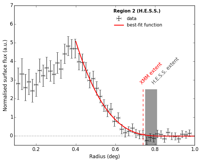
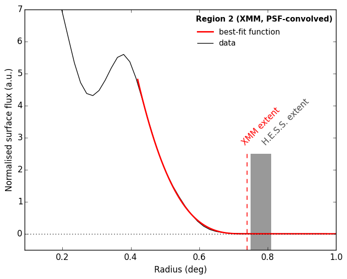
Figure 8: H.E.S.S. radial profiles from RX J1713.7$-$3946 compared to the XMM-Newton data. For wedges 1 and 2, the profiles are shown on the left in both panels. On the right, the PSF-convolved XMM-Newton profile is shown. For both profiles, the empirical best-fit function is overlaid as red solid line, see Sect. 3 for more details.

Figure 8 shows the radial profiles from the H.E.S.S and XMM-Newton maps separately together with the best-fit model functions discussed in Sect. 3.

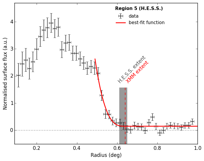
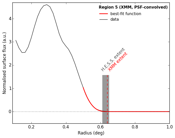
Figure 9: continued: For wedges 3-5, the H.E.S.S. radial profiles from RX J1713.7$-$3946 are shown on the left in all three panels. On the right, the PSF-convolved XMM-Newton profile is shown. For both profiles, the empirical best-fit function is overlaid as red solid line; see Sect. 3 for more details.

Appendix B H.E.S.S. image with overlaid XMM contours

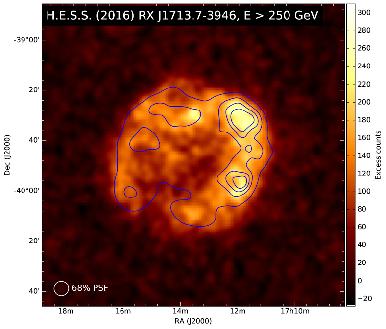
Figure 10: H.E.S.S. gamma-ray excess image of RX J1713.7$-$3946 with overlaid XMM-Newton contours (1–10 keV).

Appendix C Results from a border-detection algorithm

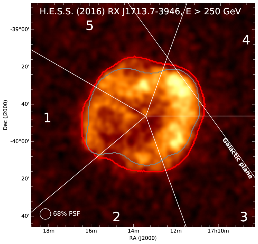
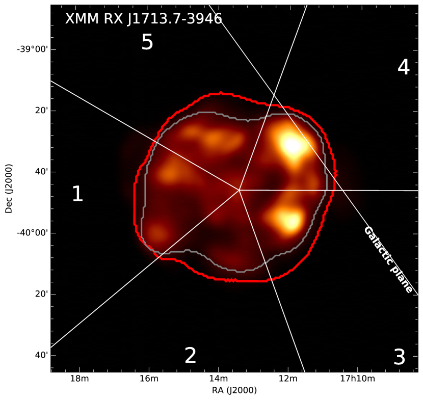
Figure 11: Results of the border-finder algorithm. On the left, the H.E.S.S. gamma-ray excess image of RX J1713.7$-$3946 is shown with overlaid borders of the gamma-ray (red) and X-ray (grey) data detected by the border-finder algorithm described in Chan & Vese (2001). The wedges in which the radial profiles in Sect. 3.2 are studied are also shown along with the Galactic plane. On the right, the same two borders are overlaid on the XMM-Newton X-ray image for comparison.

As an alternative method to determine the extent of the SNR shell the border-detection algorithm described by Chan & Vese (2001) was used on the XMM-Newton and H.E.S.S. maps. This method is widely used in image analysis to separate complex features from backgrounds. Figure 11 shows the H.E.S.S. image together with the contours of the detected borders. The largest differences between the radial sizes appear towards the south-west and towards the north. In the south-west the radial fitting method (Region 3, see Sect. 3) shows the largest differences between X-rays and VHE gamma rays. However, towards the north (Region 5), the radial sizes are consistent in the fitting method. In this area, the radial profiles are the most complex, and a diffuse emission component along the Galactic plane may play an important role. While the radial fitting approach tries to find the absolute outer edge of the shell, the border-finder algorithm interprets fainter outer structures in the X-ray map as background not belonging to the SNR shell.

Tests with the H.E.S.S. map showed that the results from the border-detection algorithm are very stable against a large range of different signal-to-noise levels as well as systematic changes of the normalisation of the H.E.S.S. background by up to 2%.

Appendix D Comparison of the radial profile between XMM-Newton and ROSAT

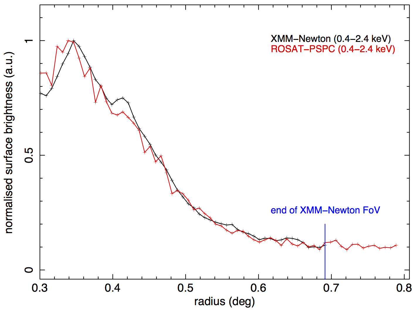
Figure 12: Radial profiles (full azimuth range) extracted from the XMM-Newton and ROSAT maps and normalised to the peak flux.

Figure 12 shows a comparison between radial profiles from XMM-Newton and ROSAT (Snowden et al. 1997). The wider coverage of ROSAT is used here to confirm that the baseline Galactic diffuse surface brightness level is already reached within the XMM-Newton FoV.

Appendix E Spectral energy distributions of the western and eastern half

Appendix F H.E.S.S. energy flux points

The energy flux points shown in Fig. 3 are given below.

E (TeV)       E low (TeV)        E high (TeV)      Flux (erg cm-2 s-1)     Flux error (erg cm-2 s-1)
 0.23          0.21               0.25             4.44e-11                8.35e-12
 0.27          0.25               0.29             3.99e-11                5.17e-12
 0.32          0.29               0.35             4.28e-11                3.52e-12
 0.38          0.35               0.41             3.92e-11                2.41e-12
 0.45          0.41               0.49             3.96e-11                2.04e-12
 0.53          0.49               0.58             3.38e-11                1.73e-12
 0.63          0.58               0.69             3.43e-11                1.41e-12
 0.75          0.69               0.81             3.41e-11                1.34e-12
 0.89          0.81               0.96             3.21e-11                1.22e-12
 1.05          0.96               1.14             2.94e-11                1.12e-12
 1.25          1.14               1.36             3.02e-11                1.09e-12
 1.48          1.36               1.61             3.25e-11                1.07e-12
 1.76          1.61               1.91             2.99e-11                1.01e-12
 2.08          1.91               2.26             3.09e-11                1.19e-12
 2.47          2.26               2.68             2.62e-11                1.24e-12
 2.93          2.68               3.18             2.54e-11                1.17e-12
 3.47          3.18               3.77             2.59e-11                1.18e-12
 4.12          3.77               4.47             2.39e-11                1.28e-12
 4.88          4.47               5.29             2.50e-11                1.23e-12
 5.79          5.29               6.28             2.34e-11                1.31e-12
 6.86          6.28               7.44             2.01e-11                1.38e-12
 8.14          7.44               8.83             1.74e-11                1.51e-12
 9.65          8.83              10.47             1.42e-11                1.53e-12
11.44         10.47              12.41             1.58e-11                1.59e-12
13.56         12.41              14.71             8.34e-12                1.70e-12
16.08         14.71              17.45             9.67e-12                1.67e-12
19.99         17.45              22.53             3.82e-12                1.41e-12
24.62         22.53              26.71             5.68e-12                1.75e-12
29.19         26.71              31.67             2.79e-12                1.57e-12
34.61         31.67              37.55             5.08e-12                1.27e-12

References

- Abdo et al. (2011) Abdo, A. A., Ackermann, M., Ajello, M., et al. 2011, ApJ, 734, 28
- Abdo et al. (2009) Abdo, A. A., Ackermann, M., Ajello, M., et al. 2009, Phys. Rev. D, 80, 122004
- Abramowski et al. (2011) Abramowski, A., Acero, F., Aharonian, F. A., et al. 2011, Physical Review Letters, 106, 161301
- Abramowski et al. (2010) Abramowski, A., Acero, F., Aharonian, F. A., et al. 2010, A&A, 520, A83
- Acero et al. (2015) Acero, F., Ackermann, M., Ajello, M., et al. 2015, ApJS, 218, 23
- Acero et al. (2016a) Acero, F., Ackermann, M., Ajello, M., et al. 2016a, ApJS, 223, 26
- Acero et al. (2016b) Acero, F., Ackermann, M., Ajello, M., et al. 2016b, ApJS, 224, 8
- Acero et al. (2009) Acero, F., Ballet, J., Decourchelle, A., et al. 2009, A&A, 505, 157
- Acharya et al. (2013) Acharya, B. S., Actis, M., Aghajani, T., et al. 2013, Astroparticle Physics, 43, 3
- Ackermann et al. (2013) Ackermann, M., Ajello, M., Allafort, A., et al. 2013, Science, 339, 807
- Aharonian (2013a) Aharonian, F. 2013a, Astrophysics at Very High Energies, Saas-Fee Advanced Course, Volume 40. ISBN 978-3-642-36133-3. Springer-Verlag Berlin Heidelberg, 2013, p. 1, 40, 1
- Aharonian (2013b) Aharonian, F. A. 2013b, Astroparticle Physics, 43, 71
- Aharonian et al. (2004) Aharonian, F. A., Akhperjanian, A. G., Aye, K.-M., et al. 2004, Nature, 432, 75
- Aharonian et al. (2008) Aharonian, F. A., Akhperjanian, A. G., Bazer-Bachi, A. R., et al. 2008, A&A, 481, 401
- Aharonian et al. (2006a) Aharonian, F. A., Akhperjanian, A. G., Bazer-Bachi, A. R., et al. 2006a, A&A, 457, 899
- Aharonian et al. (2006b) Aharonian, F. A., Akhperjanian, A. G., Bazer-Bachi, A. R., et al. 2006b, A&A, 449, 223
- Aharonian et al. (2007) Aharonian, F. A., Akhperjanian, A. G., Bazer-Bachi, A. R., et al. 2007, A&A, 464, 235
- Aharonian & Atoyan (1996) Aharonian, F. A. & Atoyan, A. M. 1996, A&A, 309, 917
- Aharonian & Atoyan (1999) Aharonian, F. A. & Atoyan, A. M. 1999, A&A, 351, 330
- Akaike (1974) Akaike, H. 1974, IEEE transactions on automatic control, 19, 716
- Axford et al. (1977) Axford, W. I., Leer, E., & Skadron, G. 1977, International Cosmic Ray Conference, 11, 132
- Bell (1978) Bell, A. R. 1978, MNRAS, 182, 147
- Bell et al. (2013) Bell, A. R., Schure, K. M., Reville, B., & Giacinti, G. 2013, MNRAS, 431, 415
- Berezhko & Völk (2006) Berezhko, E. G. & Völk, H. J. 2006, A&A, 451, 981
- Berge et al. (2007) Berge, D., Funk, S., & Hinton, J. 2007, A&A, 466, 1219
- Blandford & Ostriker (1978) Blandford, R. D. & Ostriker, J. P. 1978, ApJ, 221, L29
- Blasi (2013) Blasi, P. 2013, A&A Rev., 21, 70
- Casanova et al. (2010) Casanova, S., Jones, D. I., Aharonian, F. A., et al. 2010, PASJ, 62, 1127
- Cassam-Chenaï et al. (2004) Cassam-Chenaï, G., Decourchelle, A., Ballet, J., et al. 2004, A&A, 427, 199
- Chan & Vese (2001) Chan, T. F. & Vese, L. A. 2001, IEEE Transactions on Image Processing, 10, 266
- Chevalier (1982) Chevalier, R. A. 1982, ApJ, 258, 790
- de Naurois & Rolland (2009) de Naurois, M. & Rolland, L. 2009, Astroparticle Physics, 32, 231
- Drury (1983) Drury, L. O. 1983, Reports on Progress in Physics, 46, 973
- Drury (2011) Drury, L. O. 2011, MNRAS, 415, 1807
- Ellison et al. (2010) Ellison, D. C., Patnaude, D. J., Slane, P., & Raymond, J. 2010, ApJ, 712, 287
- Ellison et al. (2012) Ellison, D. C., Slane, P., Patnaude, D. J., & Bykov, A. M. 2012, ApJ, 744, 39
- Federici et al. (2015) Federici, S., Pohl, M., Telezhinsky, I., Wilhelm, A., & Dwarkadas, V. V. 2015, A&A, 577, A12
- Finke & Dermer (2012) Finke, J. D. & Dermer, C. D. 2012, ApJ, 751, 65
- Fukui et al. (2003) Fukui, Y., Moriguchi, Y., Tamura, K., et al. 2003, PASJ, 55, L61
- Fukui et al. (2012) Fukui, Y., Sano, H., Sato, J., et al. 2012, ApJ, 746, 82
- Funk et al. (2004) Funk, S., Hermann, G., Hinton, J., et al. 2004, Astroparticle Physics, 22, 285
- Gabici & Aharonian (2016) Gabici, S. & Aharonian, F. 2016, in European Physical Journal Web of Conferences, Vol. 121, European Physical Journal Web of Conferences, 04001
- Gabici & Aharonian (2014) Gabici, S. & Aharonian, F. A. 2014, MNRAS, 445, L70
- Gabici et al. (2009) Gabici, S., Aharonian, F. A., & Casanova, S. 2009, MNRAS, 396, 1629
- Giacalone & Jokipii (2007) Giacalone, J. & Jokipii, J. R. 2007, ApJ, 663, L41
- Ginzburg & Syrovatskii (1965) Ginzburg, V. L. & Syrovatskii, S. I. 1965, ARA&A, 3, 297
- Grenier et al. (2015) Grenier, I. A., Black, J. H., & Strong, A. W. 2015, ARA&A, 53, 199
- Hahn et al. (2014) Hahn, J., de los Reyes, R., Bernlöhr, K., et al. 2014, Astroparticle Physics, 54, 25
- H.E.S.S. Collaboration et al. (2016a) H.E.S.S. Collaboration, Abdalla, H., Abramowski, A., et al. 2016a, Deeper H.E.S.S. Observations of Vela Junior (RX J0852.04622): Morphology Studies and Resolved Spectroscopy, A&A forthcoming
- H.E.S.S. Collaboration et al. (2016b) H.E.S.S. Collaboration, Abdalla, H., Abramowski, A., et al. 2016b, The H.E.S.S. Galactic plane survey, A&A forthcoming
- H.E.S.S. Collaboration et al. (2016c) H.E.S.S. Collaboration, Abdalla, H., Abramowski, A., et al. 2016c, The supernova remnant W49B as seen with H.E.S.S. and Fermi-LAT, A&A forthcoming, arXiv:1609.00600
- Inoue et al. (2012) Inoue, T., Yamazaki, R., Inutsuka, S.-i., & Fukui, Y. 2012, ApJ, 744, 71
- Jogler & Funk (2016) Jogler, T. & Funk, S. 2016, ApJ, 816, 100
- Kafexhiu et al. (2014) Kafexhiu, E., Aharonian, F. A., Taylor, A. M., & Vila, G. S. 2014, Phys. Rev. D, 90, 123014
- Katsuda et al. (2015) Katsuda, S., Acero, F., Tominaga, N., et al. 2015, ApJ, 814, 29
- Kelner et al. (2006) Kelner, S. R., Aharonian, F. A., & Bugayov, V. V. 2006, Phys. Rev. D, 74, 034018
- Khangulyan et al. (2014) Khangulyan, D., Aharonian, F. A., & Kelner, S. R. 2014, ApJ, 783, 100
- Koyama et al. (1997) Koyama, K., Kinugasa, K., Matsuzaki, K., et al. 1997, PASJ, 49, L7
- Krymskii (1977) Krymskii, G. F. 1977, Akademiia Nauk SSSR Doklady, 234, 1306
- Lazendic et al. (2004) Lazendic, J. S., Slane, P. O., Gaensler, B. M., et al. 2004, ApJ, 602, 271
- Malkov et al. (2005) Malkov, M. A., Diamond, P. H., & Sagdeev, R. Z. 2005, ApJ, 624, L37
- Malkov et al. (2013) Malkov, M. A., Diamond, P. H., Sagdeev, R. Z., Aharonian, F. A., & Moskalenko, I. V. 2013, ApJ, 768, 73
- Maxted et al. (2013) Maxted, N. I., Rowell, G. P., Dawson, B. R., et al. 2013, PASA, 30, 55
- Morlino et al. (2009) Morlino, G., Amato, E., & Blasi, P. 2009, MNRAS, 392, 240
- Nakamori et al. (2015) Nakamori, T., Katagiri, H., Sano, H., et al. 2015, ArXiv e-prints
- Ohm et al. (2009) Ohm, S., van Eldik, C., & Egberts, K. 2009, Astroparticle Physics, 31, 383
- Olive et al. (2014) Olive, K. A. et al. 2014, Chin. Phys., C38, 090001
- Parizot et al. (2006) Parizot, E., Marcowith, A., Ballet, J., & Gallant, Y. A. 2006, A&A, 453, 387
- Parsons & Hinton (2014) Parsons, R. D. & Hinton, J. A. 2014, Astroparticle Physics, 56, 26
- Pfeffermann & Aschenbach (1996) Pfeffermann, E. & Aschenbach, B. 1996, in Roentgenstrahlung from the Universe, 267–268
- Porter et al. (2006) Porter, T. A., Moskalenko, I. V., & Strong, A. W. 2006, ApJ, 648, L29
- Shibata et al. (2011) Shibata, T., Ishikawa, T., & Sekiguchi, S. 2011, ApJ, 727, 38
- Slane et al. (1999) Slane, P., Gaensler, B. M., Dame, T. M., et al. 1999, ApJ, 525, 357
- Snowden et al. (1997) Snowden, S. L., Egger, R., Freyberg, M. J., et al. 1997, ApJ, 485, 125
- Tanaka et al. (2008) Tanaka, T., Uchiyama, Y., Aharonian, F. A., et al. 2008, ApJ, 685, 988
- Truelove & McKee (1999) Truelove, J. K. & McKee, C. F. 1999, ApJS, 120, 299
- Uchiyama et al. (2003) Uchiyama, Y., Aharonian, F. A., & Takahashi, T. 2003, A&A, 400, 567
- Uchiyama et al. (2007) Uchiyama, Y., Aharonian, F. A., Tanaka, T., Takahashi, T., & Maeda, Y. 2007, Nature, 449, 576
- Vink (2012) Vink, J. 2012, A&A Rev., 20, 49
- Zabalza (2015) Zabalza, V. 2015, in Proceedings of the 34th International Cosmic Ray Conference (ICRC 2015), in press, arXiv:1509.03319
- Zirakashvili & Aharonian (2010) Zirakashvili, V. N. & Aharonian, F. A. 2010, ApJ, 708, 965