Exoplanet Orbital Eccentricities Derived From LAMOST-Kepler Analysis

Abstract

The nearly circular (mean eccentricity $\bar{e}\sim 0.06$) and coplanar (mean mutual inclination $\bar{i}\sim 3^{\circ}$) orbits of the Solar System planets motivated Kant and Laplace to put forth the hypothesis that planets are formed in disks, which has developed into the widely accepted theory of planet formation. Surprisingly, the first several hundred extrasolar planets (mostly Jovian) discovered using the Radial Velocity (RV) technique are commonly on eccentric orbits ($\bar{e}\sim 0.3$). This raises a fundamental question: Are the Solar System and its formation special? The Kepler mission has found thousands of transiting planets dominated by sub-Neptunes, but most of their orbital eccentricities remain unknown. By using the precise spectroscopic host star parameters from the LAMOST observations, we measure the eccentricity distributions for a large (698) and homogeneous Kepler planet sample with transit duration statistics. Nearly half of the planets are in systems with single transiting planets (singles), while the other half are multiple-transiting planets (multiples). We find an eccentricity dichotomy: on average, Kepler singles are on eccentric orbits with $\bar{e}\approx$ 0.3, while the multiples are on nearly circular $(\bar{e}=0.04^{+0.03}_{-0.04})$ and coplanar $(\bar{i}={1.4}^{+0.8}_{-1.1}$ degree) orbits similar to the Solar System planets. Our results are consistent with previous studies of smaller samples and individual systems. We also show that Kepler multiples and Solar System objects follow a common relation ($\bar{e}\sim$(1-2)$\times\bar{i}$) between mean eccentricities and mutual inclinations. The prevalence of circular orbits and the common relation may imply that the Solar system is not so atypical in the Galaxy after all.

This manuscript was compiled on

-2pt

Our knowledge of orbital shapes (parameterized with eccentricities) of planetary systems has been drastically advanced in the last two decades largely thanks to the RV planet surveys, but there remain some major puzzles. For example, the majority of RV planets are found on eccentric orbits ($\bar{e}\sim 0.3$)[1] in contrast to the Solar system planets, raising a fundamental question: Is the Solar System an atypical member of the planetary system population in the Galaxy?[2] Furthermore, the RV method has some key limitations. For example, several notable biases and degeneracies can introduce considerable systematical uncertainties into the eccentricity distributions derived from the RV technique [3, 4, 5]. In addition, the majority of eccentricities measured using the RV method are for giant planets (e.g., Jupiter size), while the eccentricity distributions of smaller planets (e.g., Earth to Neptune size) remain poorly understood.

Complementary to the RV technique, the Kepler mission has discovered thousands of planet candidates down to about Earth radius using the transit technique [6]. About half of the Kepler planets are in systems with multiple transiting planets, and on average they are on nearly coplanar orbits similar to the Solar System (see review by [7]). For most transiting planets, eccentricities cannot be directly inferred from the light curves alone. Individual light-curve-based eccentricity measurements have been made for a small number of planets, most of which are systems meeting special conditions such as giant planets with high eccentricities[8], systems with precisely characterized host stars from asteroseismology [9] and highly compact and dynamically rich systems exhibiting transit timing variations (TTVs) (e.g. [10]). Analyzing TTVs for a sample of transit systems also allows to constrain eccentricity distributions[11], but this method only applies to a limited number ($\sim 100$) of systems with special (near-)resonant configurations.

Method

A robust general method to derive eccentricity distribution is based on the statistics of transit duration [12] – the time for transiting planets to cross the stellar disks. Based on Kepler’s Third Law, for a planet on a circular orbit that transits across the stellar center, the transit duration $T_{0}$ is uniquely determined by the orbital period $P$, the planet-to-star radius ratio $r=R_{p}/R_{\star}$ and stellar density $\rho_{\star}$: $T_{0}\propto P^{1/3}\rho_{\star}^{-1/3}(1+r)$. For an eccentric and inclined orbit, the transit duration $T$ depends on the eccentricity $e$ as well as the orientation of the orbit, which is described by the argument of periastron $\omega$ and the impact parameter $b$:

$$T=T_{\rm 0}\times\sqrt{(1-b^{2})(1-e^{2})}/(1+e{\rm sin}\omega)$$ (1)

$P$, $T$ and $r$ are observables that can be directly measured from the transit light curve with high precision. Using an ensemble of transiting planet systems, the distributions of $\omega$ and $b$ can be modeled and used to infer the eccentricity distribution from the statistics of $T/T_{\rm 0}$. Moreover, for systems with multiple transiting planets, the $b$ distribution also depends on the mutual orbital inclinations (Throughout this paper, inclination and the symbol $\bar{i}$ always refer to the mutual orbital inclination unless otherwise stated.) among the planets, and thus both the eccentricity and inclination distributions can be inferred. See SI Appendix, section 3, for a full description of our methodology.

This method hinges on the well-characterized host properties to derive reliable and precise stellar density $\rho_{\star}$. Due to the difficulty of precisely characterizing large samples of stars, the method has hitherto not been applied to a large and homogeneous sample of Kepler planetary systems. Previous studies such as [13] have used stellar parameters from the Kepler input catalog (KIC), which are plagued by large systematic uncertainties (see SI Appendix, section 1). A recent study [9] uses a sample of 28 multi-transiting systems with precisely measured stellar densities from asteroseismology, and found that the planetary orbits in these systems have low eccentricities. The sample was nevertheless biased towards systems with asteroseismic detections, and did not include single transiting planets.

Results

Here, we derive the eccentricity distributions of 698 Kepler planet candidates using transit duration statistics. The analysis of this large and homogeneous sample [14] is made possible through spectroscopic observations by the Large Sky Area Multi-Object Fiber Spectroscopic Telescope (LAMOST)[15, 16] with reliably derived stellar properties [17] from the LAMOST Stellar Parameter (LASP) pipeline (see Sec 4.4 of [16] and also [18]). See SI Appendix Section 1 for further discussions on stellar parameters.

Eccentricity Dichotomy

Our sample consists of 368 systems with single transiting planet candidates ($N_{p}=1$) and 330 planet candidates in multiples ($N_{p}>1$). For the two subsamples, we simulate $T/T_{\rm 0}$ distributions with various $\bar{e}$ and/or $\bar{i}$ assuming Rayleigh distributions, and fit them to the observed $T/T_{\rm 0}$ distributions (see SI Appendix Section 4). The results are shown in Fig. 1 and 2 for the singles and multiples, respectively.

The eccentricity distribution of singles is clearly non-circular with a mean eccentricity of $\bar{e}=0.32\pm 0.02$. In contrast, the orbits of multiples are consistent with being circular and nearly coplanar, with a mean eccentricity $\bar{e}<0.07$ and a mean orbital inclinations 0.006 rad (0.3^∘)$<\bar{i}<$0.038 rad (2.2^∘). We further divide the multiples into subsamples with $N_{p}=2$, $N_{p}=3$ and $N_{p}>3$ transiting planets. We find that the mean eccentricities of these three subsamples are all close to zero and comparable to each other within statistical uncertainties, in contrast to the large mean eccentricity of singles (Fig. 3). Our results indicate an abrupt transition of $\bar{e}$ from singles ($N_{p}=1$) to multiples ($N_{p}>1$) rather than a smooth correlation with $N_{p}$ as suggested from the study on the RV sample[19]. The low eccentricities of multiples found here are consistent with previous studies of smaller samples[9, 20, 11] and individual systems, e.g., Kepler-11[10], Kepler-36[21] etc.

Singles: Two Populations

When viewed from different orientations, a multiple-planet system can result in multi-transiting and single-transiting systems. Our results provide a direct evidence that not all Kepler single-transiting system come from the same underlying planet population as the systems with multiple transiting planets. Instead, the Kepler planet population is likely dichotomic in eccentricities: at least some of the single-transits come from a dynamically hotter population than the underlying population of multi-transiting systems.

We are therefore motivated to investigate the transit duration ratio of singles with a two-population model (Fig. 4). In the model, we fix the dynamically cold population with an eccentricity distribution corresponding to the best fit of multi-transiting systems, and fit the fraction ($F_{hot}$) and mean eccentricity ($\bar{e}_{hot}$) of the hot population. The best-fit two-population model provides a statistically significant improvement over the one-population model in matching the observations. We find that the hot population makes up a small fraction of the sample ($F_{hot}\sim 16\%-36\%$) with an even higher mean eccentricity ($\bar{e}_{hot}>0.47$), indicating that the singles are probably dominated by a cold population ($F_{cold}=1-F_{hot}\sim 64\%-84\%$).

Prevalence of Circular Orbits

As the singles contribute to about half of all the Kepler planets, the fraction of planets in the cold population out of the whole sample is even higher ($\sim 80\%-90\%$), leading to a conclusion that most Kepler planets are on near-circular orbits. The dominance of near-circular orbits may imply that planets mostly form and evolve in a relatively gentle manner dynamically. Violent dynamical scenarios which excite high eccentricities, for example through planet-planet scattering[22] and close stellar encounters[23], therefore must be relatively rare, unless there are subsequent processes that efficiently circularize the orbits.

A common relation between eccentricity and inclination

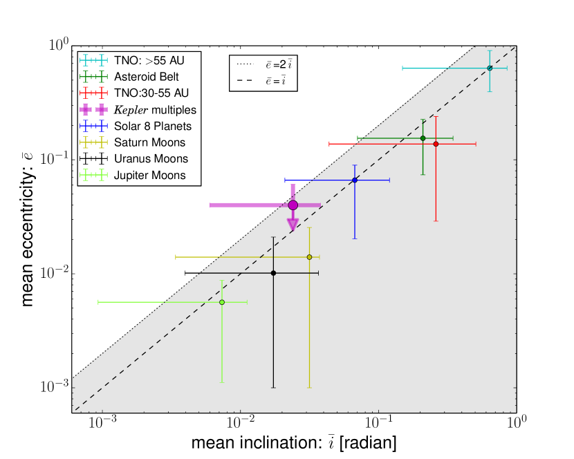
Figure 5: The mean eccentricity and inclination of Kepler multiples fit into the pattern of the Solar System objects. The thin filled circle and error bars show the mean values and 68% confidence intervals of orbital eccentricity and inclination distributions for Solar System objects, including 8 planets (blue), regular moons of Jupiter, Saturn and Uranus (light green, yellow and black), main belt asteroids (green) and Trans-Neptune objects (TNOs – both the classical Kuiper Belt objects with orbital semi-major axes 30-55 AU shown in red and the scattered disk objects with semi-major axes $>$55 AU shown in cyan). They follow an approximately linear relation with $\bar{e}\sim$(1-2)$\times\bar{i}$ (dashed and dotted lines). The thick purple filled circle, error bar (and arrow) show the eccentricity and inclination constraints of Kepler multiples: 0.006 rad (0.3^∘)$<\bar{i}<$0.038 rad (2.2^∘) and $\bar{e}<0.07$ derived in this work. The Kepler multiples fall on the linear relation of the Solar System objects, and they are on similarly circular and coplanar orbits as the Solar System planets.

The low eccentricities and inclinations of the Kepler multiples are naturally expected from simple considerations of terrestrial planet formation [24], and they are consistent with the expectation from the well-established coplanarity of the Kepler multiple systems ($\bar{i}\sim$ a few degrees)[25, 26], resembling the Solar System planets. Further comparing the orbital properties of Kepler multiples to those of the Solar System objects, we find an intriguing pattern: orbital eccentricities and inclinations are distributed around $\bar{e}\sim$(1-2)$\times\bar{i}$ (see Fig. 5). All the regular moon systems are located in the dynamically cold end (bottom left), while the Asteroid Belt objects and Trans-Neptune objects (TNOs) are located in the dynamically hot end (up-right). Interestingly, the Kepler planets and the Solar System planets ($\bar{e}\sim 0.06$, $\bar{i}\sim 3^{\circ}$) are located in the intermediate region and close to each other. Note that the Kepler single-transiting systems are not shown in Fig. 5 because we cannot measure their inclination distributions. If they were following the same pattern, they would be located in the dynamical hot region (up right corner of Fig. 5) given their large mean eccentricity. If true, we would expect that the obliquity of Kepler single transiting systems should be systematically larger than those of the Kepler multiples[27].

Discussions

In contrast to the low eccentricity of multiple-transit systems, the mean eccentricity of single-transit systems is much higher and similar to that of planets found by RV surveys, but unlike the RV planets, most of the Kepler single-transiting systems are sub-Neptune-sized planets ($<4$ Earth radii). We further compare the singles to the multiples in terms of planetary properties (radius and orbital period) and host properties (stellar mass, radius, metallicity and surface density). We found that these parameters are unlikely to play a decisive role in forming the eccentricity dichotomy (SI Appendix section 2.1). The dichotomy may have important implications for planet formation and evolution. From the perspective of evolution, current studies have found that the architecture of a planetary system may depend on various conditions during planet formation, e.g., the total mass and distribution of solid[28] and the degree of depletion of gas[29] in the planet-forming disk. From the perspective of evolution, long-term planet-planet interactions can sculpt the planet architectures [30, 31, 32] after planet formation. The eccentricity dichotomy found in this work may help to pin down the initial conditions for planet formation and shed light on planet dynamical evolution.

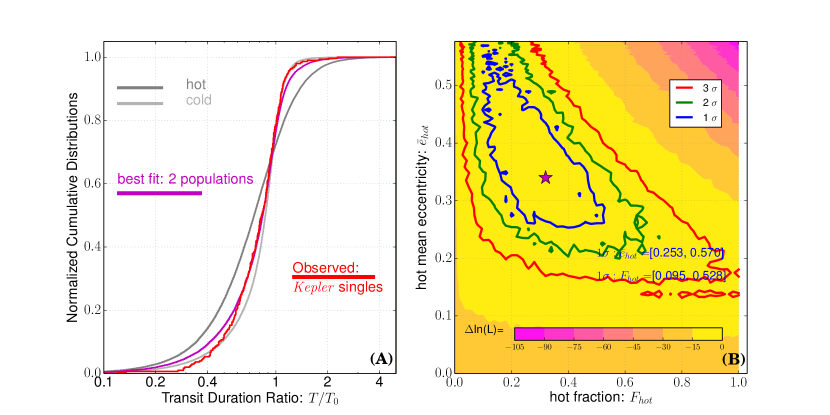
Figure S13: Similar to Fig.4, but here we cut off observed KOIs with large false positive probability (FPP$>$68.3%). For comparison, we also plot the transit duration ratio distributions of a hot ($\bar{e}$=0.6) and cold ($\bar{e}$=0.04) populations in the left panel.

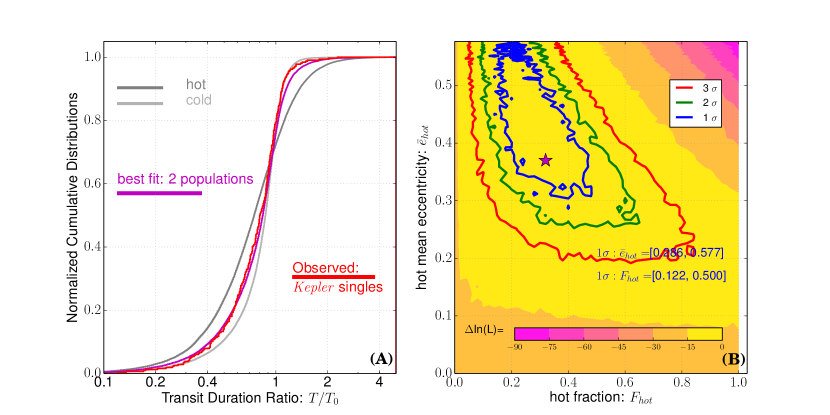
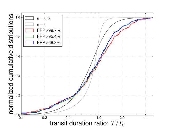
Figure S14: Similar to Fig.4, but here we cut off observed KOIs with large false positive probability (FPP$>$95.4%). For comparison, we also plot the transit duration ratio distributions of a hot ($\bar{e}$=0.6) and cold ($\bar{e}$=0.04) populations in the left panel.

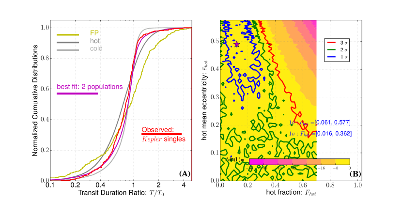
Figure S16: Similar to Fig.4, but here we add in our model a fix component (12% in fraction) with transit duration ratio distribution drawn from that of false positives (FPP>95.4%). For comparison, we also plot the transit duration ratio distributions of the false positive, the hot ($\bar{e}$=0.6) and cold ($\bar{e}$=0.04) populations in the left panel. In the right panel, the contour map is truncated because the hot fraction varies in a smaller range between 0 and 0.7 in our simulation.

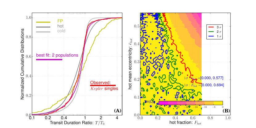
Figure S17: Similar to Fig.S16, but here we add in our model a fix component (12% in fraction) with transit duration ratio distribution drawn from that of false positives (FPP>99.7%).

One important concern about the eccentricity dichotomy is the likely larger false positive (FP) rate of the singles as compared to that of the multiples. To investigate this issue, we perform two sets of analyses (see SI Appendix section 5.4). In the first set of analysis, we remove singles with large FP probability to reduce the total FP rate of single sample to a degree (a few percents) that is comparable to that of the multiple sample. In the other analysis, we model the effects of the FP on transit duration ratio distribution by injecting FPs into our simulations and fit the data. Both analyses lead to results (SI Appendix Fig.S13, Fig.S14, Fig.S16 and Fig.S17) that are consistent with those shown in Fig. 4. Based on these analyses, we conclude that FP should not qualitatively change our main conclusion, namely the Kepler singles are composed of dynamically cold and dynamically hot populations.

The correlation between eccentricities and inclinations shown in Fig. 5 is generally expected from popular planet formation models, which predict that orbital eccentricities are less than twice of orbital inclinations on average[33] (the grey region in Fig. 5). In fact, $\bar{e}\sim 2\bar{i}$ is consistent with the prediction of energy equipartition among the various degrees of freedom of planetary orbit[34]. The prevalence of circular orbits among Kepler planets and the common pattern between Kepler multiples and Solar System planets may imply that our planetary system is not so atypical in the Galaxy after all.

We thankA. Gould, S. Tremaine, Y. Lithwick, D. Fabrycky, T. Morton, and Re’em Sari for helpful discussions. J.-W.X. and J.-L.Z. acknowledge support from the Key Development Program of Basic Research of China (973 Program, Grant 2013CB834900) and the National Natural Science Foundation of China (NSFC) (Grants 11333002). J.-W.X. is also supported by the NSFC Grant 11403012 and a Foundation for the Author of National Excellent Doctoral Dissertation of People’s Republic of China. S.D. and J.-L.Z. are supported by the Strategic Priority Research Program, The Emergence of Cosmological Structures of the Chinese Academy of Sciences (Grant XDB09000000). S.D. also acknowledges the Project 11573003 supported by NSFC. The LAMOST Fellowship is supported by Special Funding for Advanced Users, budgeted and administrated by Center for Astronomical Mega-Science, Chinese Academy of Sciences. J.F. acknowledges the support of the Joint Fund of Astronomy of NSFC and Chinese Academy of Sciences through Grant U1231202 and the National Basic Research Program of China (973 Program, Grants 2014CB845700 and 2013CB834900). Y. Wu acknowledges the NSFC under Grant 11403056. H.-G.L. is supported by the NSFC Grant 11503009. Hui Zhang is supported by the NSFC Grant 11673011. This work uses the data from the Guoshoujing Telescope (LAMOST), which is a National Major Scientific Project built by the Chinese Academy of Sciences. Funding for the project has been provided by the National Development and Reform Commission. LAMOST is operated and managed by the National Astronomical Observatories, Chinese Academy of Sciences. Z. Zhu is a Hubble Fellow.

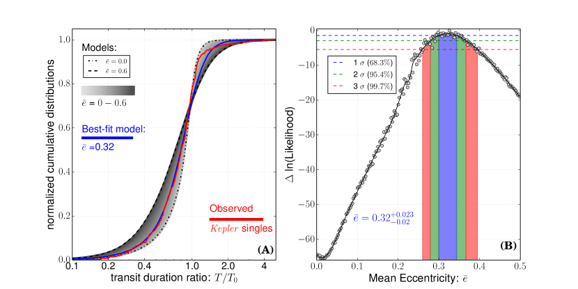
Figure 1: Transit duration ratio statistics of Kepler single transiting planets. (A) The cumulative distribution of the observed transit duration $T$ normalized by the expected values for circular and edge-on orbit $T_{0}$ for the Kepler singles (red). The circular-orbit model (dotted-dashed) is clearly ruled out. The models shown (grey scale) assume Rayleigh eccentricity distributions with mean eccentricities $\bar{e}$ varying between 0 and 0.6 (dashed). The best-fit model with $\bar{e}=0.32$ is shown in blue. The observed distribution has relatively large deviations from the best-fit model in the range of $T/T_{0}\sim 1.0-2.0$, which may indicate either the breakdown of the assumed model Rayleigh distribution or the need for more than one underlying populations (see Fig. 4 and related discussion in the main text). (B) Relative likelihood in logarithm as a function of $\bar{e}$. The blue, green and red hatched regions indicate the 68.3% ($1\sigma$) 95.4% ($2\sigma$) and 99.7% ($3\sigma$) confidence levels.

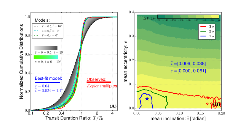
Figure 2: Transit duration ratio statistics of Kepler multiple transiting planets. (A) Cumulative distribution of observed transit duration ratios $T/T_{0}$ for Kepler multiples is shown in red. It is fitted with models assuming Rayleigh distributions in eccentricities and mutual inclinations. A range of circular-orbit models with $\bar{e}=0$ and $\bar{i}$ between 0 and $10^{\circ}$ are shown in green. The orbits of Kepler multiples are consistent with being circular and nearly coplanar. The best-fit model (blue) has $\bar{e}=0.04$ and $\bar{i}=0.024(1.4^{\circ})$. For comparison, a range of models with mean eccentricities between 0 and 0.5 and inclinations between 0 and 10 degrees are shown in grey scale. (B) Contours of relative likelihood in logarithm in the $\bar{i}-\bar{e}$ plane. The blue, green and red contours indicate the 68.3% ($1\sigma$) 95.4% ($2\sigma$) and 99.7% ($3\sigma$) confidence levels of $\bar{e}$ and $\bar{i}$. The blue star marks the best-fit values.

Figure 3: Mean eccentricity $\bar{e}$ (blue markers) and inclination $\bar{i}$ (red markers) as a function of transiting multiplicity $N_{p}$. The filled circles show the best fit and the error bars indicate the 68% confidence interval. As can be seen, it reveals an abrupt transition of $\bar{e}$ rather than a smooth correlation with $N_{p}$ (see more discussion in SI Appendix section 5.1).

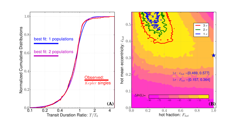
Figure 4: Modeling transit duration ratio distribution ($T/T_{0}$) of single transiting systems with a two-population model. (A) Similar to the left panel of Fig. 1 except that we model the observed distribution with a two-population model. We fix the dynamical cold population with an eccentricity distribution corresponding to the best fit of multiples as shown in Fig. 2 and set another dynamically hot population with Rayleigh eccentricity distribution with mean $\bar{e}_{hot}$. The fraction ($F_{hot}$) and mean eccentricity ($\bar{e}_{hot}$) of the hot population are two free parameters. Note that the Rayleigh distribution approaches the thermal distribution at $\bar{e}\gtrsim 0.6$. (B) Contours of relative likelihood in logarithm in the $F_{hot}-\bar{e}_{hot}$ plane. The blue, green and red hatched regions indicate the 68.3% ($1\sigma$) 95.4% ($2\sigma$) and 99.7% ($3\sigma$) confidence levels. The magenta line (left panel) and magenta star symbol (right panel) indicate the best fit of the two-population model, while the blue ones are for the one-population model. The differences in BIC (Bayesian Information Criterion) between the best fits of the one-population and two-population models is $\Delta BIC=-2\Delta{\rm ln({\bf L})}-{\rm ln}(N_{obs})$ = 40.2, which indicates a significant improvement in fitting.

Supporting Information (SI) Appendix

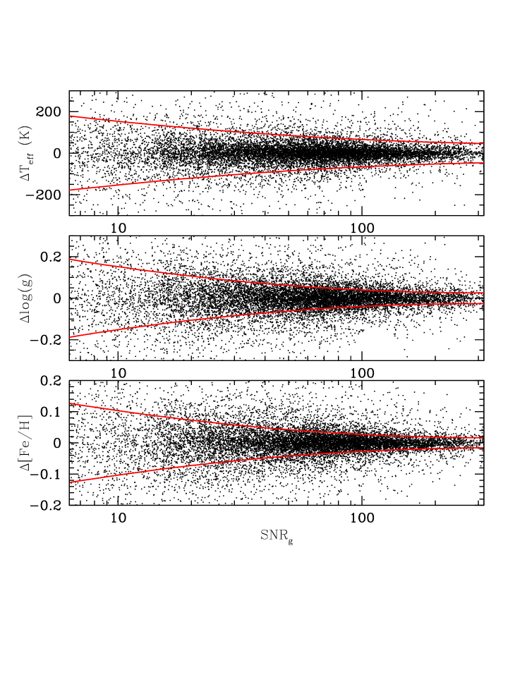
Figure S1: Internal calibration of LAMOST/LASP stellar parameter uncertainties. The unbiased estimators defined in Supplementary Sec. 1 in $T_{\rm eff}$, $log(g)$, [Fe/H] from the repeated observations as a function of SNR_g. The $68.3\%$ confidence levels in the $\log({\rm SNR}_{g})$ bins are well described by second-order polynomials as a function of $\log({\rm SNR}_{g})$ plotted in red solid lines. Note the points are for internal errors and curves describing the internal errors as a function of SNR are later combined with external errors added in quadrature to produce the final error bars (see Fig. S2).

Table of Contents
(1) Stellar Parameters. (Fig.S1-S4)

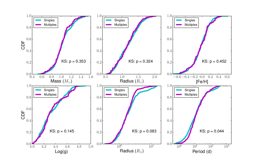
Figure S5: Normalized cumulative distributions of stellar (mass, radius, metallicity and surface gravity) and planetary (radius and orbital period) properties. The singles in our sample are shown in cyan and multiples are shown in magenta. In each panel, the $p$ value of the two-sample KS test for the distributions of singles and multiples is shown at bottom right. (See more discussions in Supporting Information Sec. 2.1)

(2) The Sample.
2.1 Singles vs. Multiples. (Fig. S5)
2.2 Comparison with the RV Sample. (Fig. S6)
2.3 Comparison with Previous Studies. (Fig. S7)

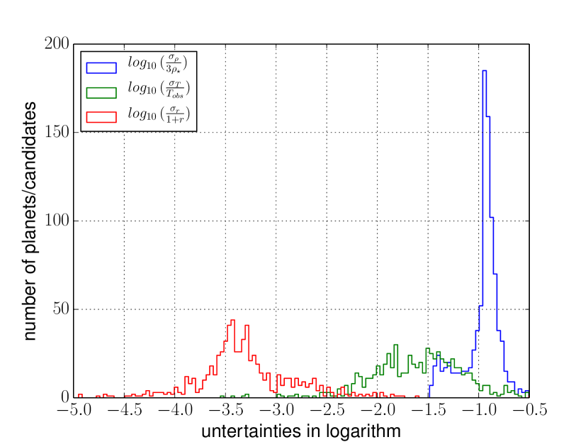
Figure S8: Three sources uncertainty (equation S15) from the measurements of transit duration $\frac{\sigma_{T}}{T_{obs}}$, stellar density $\frac{\sigma_{\rho}}{3\rho_{\star}}$ and planet/star radius ratio $\frac{\sigma_{r}}{1+r}$ .

(3) Simulations of Transit Duration Ratio Distribution. (Fig. S8)
3.1 Single Transiting Systems.
3.2 Multiple Transiting Systems.

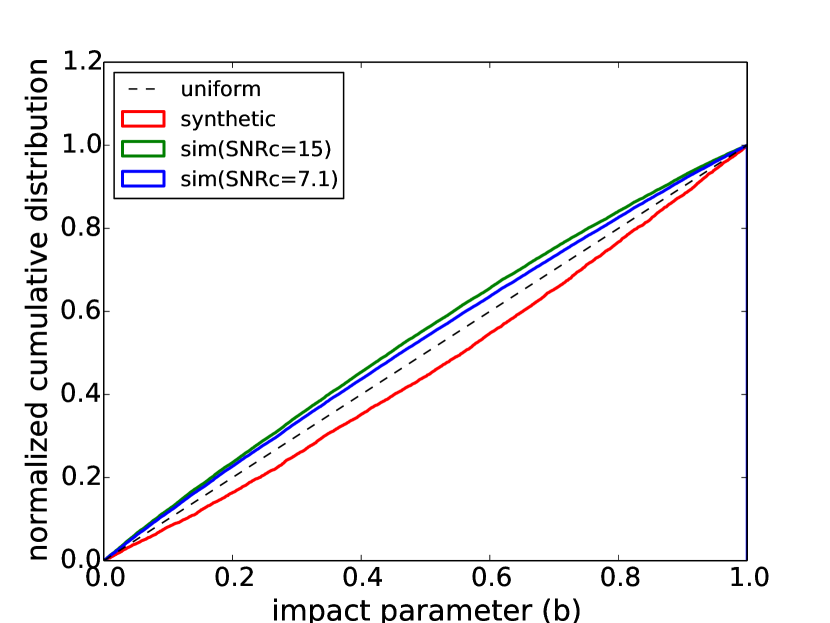
Figure S9: Transit impact parameter distributions of single transiting systems. The blue and green curves depict the distributions resulting from our nominal simulations with signal noise ratio cuts, SNRc=7.1 and SNRc=15 (see Supporting Information Sec. 3.1 and 5.5). The red curve is the one generated from a synthetic model discussed in Supporting Information Sec. 5.2), and the black dashed line shows the uniform distribution for comparison.

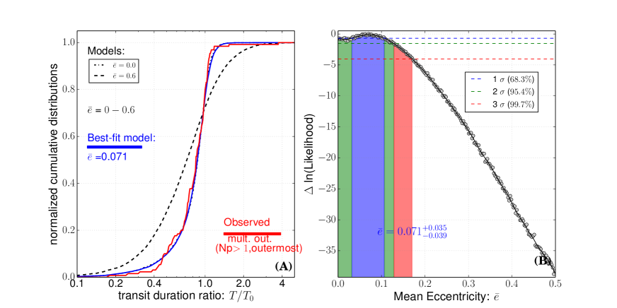
Figure S10: Similar to Fig. 1 in the main text except showing the results for the outermost transits in multiple transiting systems. (See more discussions in Supporting Information Sec. 5.3).

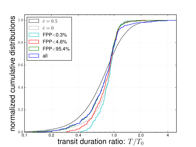
Figure S11: Transit duration ratio distribution of single transiting KOIs with false positive probabilities (FPP) less than 95.4%, 4.6% and 0.3%. For comparison, We also plot the distribution of all singles without the FPP cut and the modeling distributions with $\bar{e}=0$ and $\bar{e}=0.5$.

(4) Transit Duration Ratio: Observations vs. Simulations.
4.1 Single Transiting Systems.
4.2 Multiple Transiting Systems.
(5) Further Discussions.
5.1 An Abrupt Transition or A Smooth Correlation?
5.2 Impact Parameter Distribution. (Fig. S9)
5.3 Singles vs. the Outermost of Multiples. (Fig. S10)
5.4 False Positive.(Fig. S11-S17)
5.5 Signal-to-Noise Ratio.
5.6 Stellar Property Calibrator.

1 Stellar Parameters

LAMOST has been performing large-scale Galactic surveys with the spectral resolution $R\sim 1800$ [35, 36], and the LAMOST observations of the Kepler field started in 2011 [14]. We use the stellar parameters extracted from the LAMOST Stellar Parameter Pipeline (LASP) (see Sec 4.4 of [16] and also [18]) in the “AFGK high quality stellar parameter catalog” of LAMOST DR1, DR2 and DR3-alpha data releases. There are 29553 unique Kepler targets that have LAMOST/LASP stellar parameters. We perform several internal and external examinations on the accuracy of LAMOST/LASP stellar parameters for the dwarfs.

There are 5924 Kepler targets that have LAMOST/LASP stellar parameters from more than one epochs of LAMOST observations. We assess the internal errors by making comparisons of the multi-epoch observations for the same objects. We use the unbiased estimator [37] $\Delta Q_{i}=\sqrt{n/(n-1)}(Q_{i}-\bar{Q})$ , with $i=1,2,...,n$, where $i$ denotes each of the individual measurement of $n$ repeated measurements for the stellar parameter $Q$ for each star. Fig. S1 shows $\Delta{T_{\rm eff}}$, $\Delta{log(g)}$ and $\Delta{\rm[Fe/H]}$ using the unbiased estimator (black dots). We calculate the $68.3\%$ confidence interval in various bins of $g$-band Signal-to-Noise-Ratio per pixel (SNR_g) from LAMOST/LASP and find that they are well described by the second-order polynomials as a function of SNR_g shown in Fig. S1. For measurements with high SNR (${\rm SNR}_{g}>50$), the internal errors in $T_{\rm eff}$, $log(g)$ and [Fe/H] are less than $35$K, $0.05\,$dex and $0.03\,$dex, respectively.

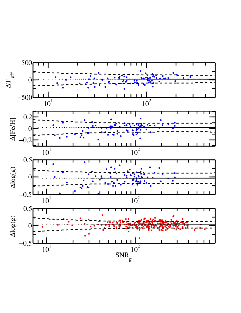
Figure S2: External calibration of LAMOST/LASP stellar parameter uncertainties for dwarfs. The top 3 panels show comparisons in $T_{\rm eff}$, $log(g)$ and [Fe/H] between LAMOST/LASP and SPC method for high-resolution spectra [38] and the bottom panel shows the comparison in $log(g)$ with asteroseismology [39]. The dotted line shows the mean and the dashed line shows the dispersion taking both internal and external uncertainties into account.

Following a previous approach of external examination of LAMOST/LASP stellar parameters [17], we compare the LAMOST/LASP parameters with those obtained from the high-resolution spectroscopy with the SPC method [38]. There are 87 stars in common between the SPC and LAMOST/LASP samples. The results of the comparison are shown in the top three panels of Fig. S2. The mean differences are small: ${\Delta{T_{\rm eff}}}=27K$, ${\Delta{log(g)}}=-0.04{\,\rm dex}$, ${\Delta{{\rm[Fe/H]}}}=0.015{\,\rm dex}$, respectively. For those with ${\rm SNR}_{g}>50$, the standard deviations in $\Delta{T_{\rm eff}}$, $\Delta{log(g)}$, $\Delta{\rm[Fe/H]}$ are $101K$, $0.15{\,\rm dex}$, $0.074{\,\rm dex}$, respectively. Because there are a small number of common stars with low SNRs, it is difficult to calibrate the errors directly from external calibrators for low-SNR measurements. In order to estimate the error bars for both high- and low-SNR measurements, the standard deviations derived from high-SNR measurements are added in quadrature with the internal error bars in the form of the second-order polynomials shown in Fig. S1. Since the standard deviations for high-SNR measurements from the external calibrations are much larger than the internal errors at similar SNRs, this approach keeps external error calibrations at high SNRs while takes the internal calibrations into account for low-SNR measurements.

We have also made comparisons in $log(g)$ with the Kepler asteroseismology sample for solar-type stars [39]. There are 260 common stars between the LAMOST/LASP and the seismology samples. We find that the $log(g)$ determinations from LAMOST/LASP are in excellent agreement with asteroseismic values, with $\Delta{log(g)}=0.03\pm 0.09$ for ${\rm SNR}_{g}>50$ (see the red points in the bottom panel of Fig. S2). The dispersion (0.09 dex) is smaller than that from the comparison with the spectroscopic sample (0.15 dex). The larger dispersion for the latter likely reflects the systematic uncertainties in the SPC method, as demonstrated by comparison with the Kepler seismology sample [40]. We apply the same quadrature corrections taking into account for the internal errors and the resulting values as a function of SNR are shown in Fig. S2 (dashed line in the bottom panel). Note that similar comparisons have been made before for LAMOST $log(g)$ but mostly for giant stars [41] or a mixture of giant and dwarf stars [16]. For giant stars, LAMOST $log(g)$ appears to have larger uncertainties compared to that for the results for the dwarfs studied here.

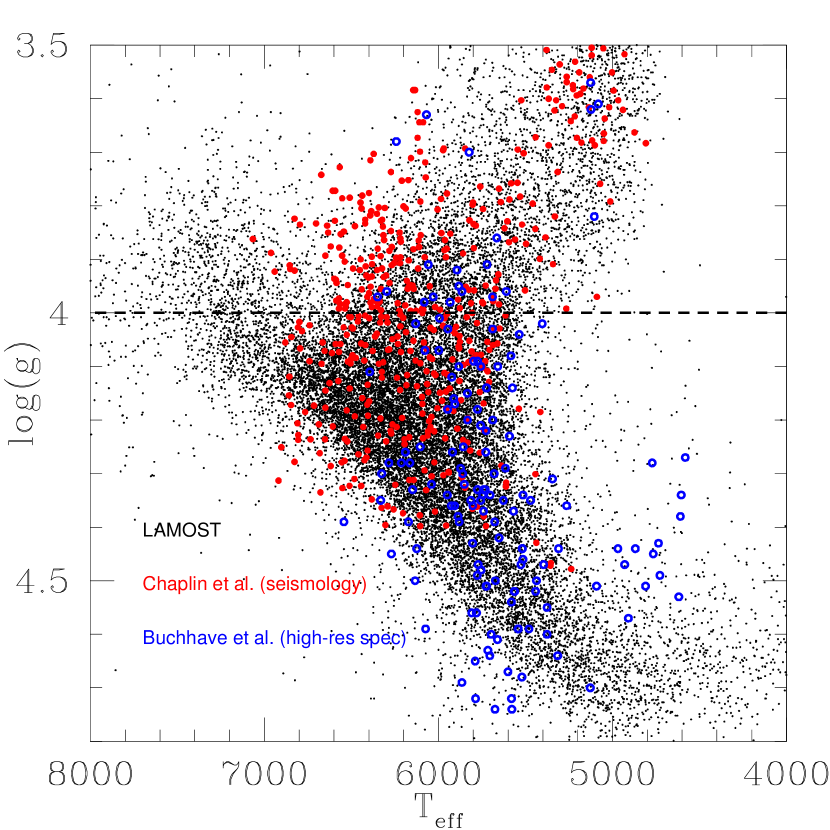
Figure S3: $T_{\rm eff}$ and $log(g)$ distribution for the LAMOST/LASP and two external stellar parameter calibration samples. LAMOST stars in the Kepler field are shown in black dots, the asteroseismology sample [39] in red solid circles and the high-resolution spectroscopic sample [38] in blue open circles. The sample used in this work has $log(g)$ larger than $4$, which is shown in black dashed line.

Fig. S3 shows the $T_{\rm eff}$ and $log(g)$ distributions of the LAMOST (black), high-resolution spectroscopy (blue) and asteroseismology (red) samples discussed above. For the planet hosts studied in our main work, we only include dwarfs with $log(g)>4$ ($log(g)=4$ is shown as dashed line). Even though asteroseismology provides higher precision in $log(g)$ than high-resolution spectroscopy, the available seismology stars cover poorly for $log(g)>4.4$ thus possibly limiting the parameter space for its applicability. Given the limitation for both calibrators, we adopt two sets of $log(g)$ with uncertainties determined from high-resolution spectroscopy and seismology respectively, and we derive the eccentricity distributions using both sets of $log(g)$ uncertainties separately. We have also make similar comparisons with the SPC sample published in 2014 [42], and there are twice as many common stars available as compared to the 2012 sample [38] used above. The mean differences and standard deviations of $\Delta{T_{\rm eff}},\Delta{log(g)},\Delta{\rm[Fe/H]}$ are $15K\pm 111K,-0.04\pm 0.15,-0.05\pm 0.14$ for the 2014 sample. The standard deviations in $\Delta{T_{\rm eff}}$ and $\Delta{log(g)}$ are similar to the 2012 sample while twice larger in [Fe/H]. This likely due to the new prior in $log(g)$ introduced to the 2014 study [42] and the covariance between $log(g)$ and [Fe/H]. In this work, we adopt the uncertainties derived from earlier SPC sample [38].

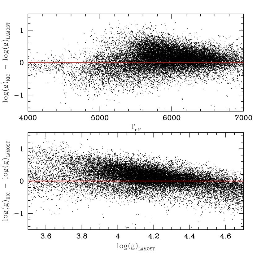
Figure S4: Comparison between KIC and LAMOST $log(g)$ reveals large uncertainties and systematics in the KIC determinations. The difference between KIC and LAMOST $log(g)$ are shown as a function of $T_{\rm eff}$ and $log(g)$ determined from LAMOST. There are not only large dispersion but also large systematic trend, in particular as a function of $log(g)$.

Fig. S4 shows the comparison in $log(g)$ between the Kepler input catalog (KIC) [43] and LAMOST/LASP. KIC stellar parameters are widely used for studies of Kepler planets, including previous studies of Kepler planet distributions using transit duration statistics [13]. From the comparison, for stars with $log(g)_{\rm LAMOST}>3.5$, the standard deviation of $\Delta{log(g)}=log(g)_{\rm KIC}-log(g)_{\rm LAMOST}$ is 0.3 dex, translating to 0.45 dex in uncertainties for $\rho_{*}$. In addition, there are serious trends of $\Delta{log(g)}$ as a function of stellar parameters, in particular $log(g)$. The average $\Delta{log(g)}$ is close to zero for stars with close to solar gravity $log(g)\sim 4.4$, but for the stars bigger than the Sun, the KIC $log(g)$ values tend to be under-estimated while for the stars smaller than the Sun, the KIC $log(g)$ tend to be over-estimated. The dynamical range of KIC $log(g)$ is smaller than the spectroscopic $log(g)$. The large dispersion and severe systematic render any statistical studies based on KIC $log(g)$ likely untrustworthy.

We determine the stellar mass, radius and density with the LAMOST/LASP $T_{\rm eff}$, $log(g)$, ${\rm[Fe/H]}$ using isochrone fitting on a dense grid of isochrones. We use the 2012 version of the interpolated isochrones from “The Dartmouth Stellar Evolution Database” [44] with a range of [Fe/H] from -1.5 dex to 0.5 dex (grid size of 0.02 dex) and stellar age from 1 to 13 Gyrs (grid size of 0.5 dex). We have also applied a separate method [45] with the Dartmouth isochrones and found good consistency between the two.

2 The Sample

We adopt the transit parameters from the cumulative Kepler planet candidate catalog reported at the NASA Exoplanet Archive (exoplanetarchive.ipac.caltech.edu; retrieved on June 29th, 2015). We crossmatch the Kepler planet candidates with LAMOST data releases discussed above, and there are 941 planet candidates with host stars characterized by the LAMOST spectroscopy. We further rule out those unusual large candidates (radius $R_{p}>$ 15 Earth radii) and those with too low transit signal noise ratio (SNR$<7.1$) (more discussion on the cuts on planet parameters in Section 5.4 and 5.5) and sub-giant/giant hosts (surface gravity $log(g)<$4), which have relatively large false positive rate[46]. We also rule out a handful of candidates with less than 3 transit, as the number of transit is too few to obtain accurate orbital period. After the cuts, we have a final sample of 698 planet candidates orbiting 501 stars. The stellar and planetary properties can be accessed from the Supplementary dataset.

2.1 2.1 Singles vs. Multiples

Our sample consists of 368 and 330 planet candidates in single and multiple transiting systems, respectively. The multiplicity rate is about $47\%$, which is comparable to that of the total Kepler sample ($42\%$ if applying the same cuts above), showing that LAMOST observations were unbiased with respect to singles or multiples as compared to the full Kepler sample. In Fig. S5, we compare various properties (stellar and planetary) for the two subsets. All stellar parameters are from the LAMOST spectral characterizations. The planet orbital periods are adopted from the Kepler catalog. The planet radii are calculated via $R_{p}=R_{\star}*r$ with $R_{\star}$ adopted derived from LAMOST and the ratio of planet and star radius, $r$, from the Kepler catalog. There appears to be no significant difference (i.e., KS p value $<$5%) between the singles and multiple in terms of stellar mass, radius, metallicity, surface gravity, except for planetary radius and orbital period. If we further cut the sample to eliminate those candidates in the regime with relatively high false positive rate (i.e., $R_{p}>6R_{\oplus}$ and orbital period $P<$ 3 day), we find that the differences in various parameters between singles and multiples are even smaller. As we show below (Section 4 and 5), these two populations however differ substantially in their transit duration ratio distributions and thus their orbital eccentricities.

2.2 2.2 Comparison with the RV Sample

From the Exoplanet Orbit Database (exoplanets.org) [1], we find 439 RV planets. Fig. S6 shows the distributions of planetary mass in the RV sample and the estimated mass assuming a simple mass-radius relation from our sample. We see that the two samples occupy different part of parameter space. The RV sample is primarily composed of giant planets, while our sample contains mainly small planets (Earth to super-Earths and/or sub-Neptunes).

2.3 2.3 Comparison to Previous Studies

Recently, Hadden & Lithwick (2014)[11] have extracted the eccentricity distribution of 139 near-resonance Kepler planets/candidates from transit timing variation (TTV sample). They find the orbits of these near-resonance planets are nearly circular with mean eccentricity $\bar{e}\sim 0.02$. Van Eylen & Albrecht (2015)[9] have derived the orbital eccentricities of 66 Kepler planets (candidates) in 28 multiple transiting systems whose host stars are characterized by asteroseismology (seismology sample). They also find these multiple systems are generally with small eccentricities. Shabram et al. 2015[47] have calculated the eccentricities of 50 short period Kepler planets (candidates) by occultation (i.e., secondary eclipse) (occultation sample). They find that the mean eccentricity is about 0.08 and a two-component model provides a better fit.

In Fig. S7, we compare our sample (LAMOST sample) to the samples of these previous studies, in terms of stellar and planetary properties. The stars in the seismology sample are biased toward sub-giants. Due to the requirements for having occultation, the occultation sample contains mostly giant planets on short orbital period, in contrast with the predominantly sub-Neptune planets of the whole Kepler planet sample and our sample. We note that [48] also studied the eccentricity distribution of Kepler giant planets and found that it was consistent with that derived from RV giant planets. Due to the TTV detection limit, the TTV sample are restricted to planets with relatively large radius (larger radius corresponds to higher SNR) and intermediate period (shorter period corresponds to shorter transit duration, longer period corresponds to fewer transit). Furthermore, TTV studies are restricted to special orbital configurations of near-resonance. In contrast, the host stars and planets in the LAMOST sample are broadly distributed and represent an unbiased and homogeneous sample from Kepler.

3 Simulations of Transit Duration Ratio Distribution

In this Section, we describe the method and procedure that are used to model the transit duration ratio distribution. Compared to previous studies[13], there are two major improvements in our modeling. Moorhead et al. [13] stressed the importance of uncertainties of stellar and transit parameters in modeling transit duration ratio but they did not take these uncertainties into account when comparing with observation. We include the uncertainties in our modeling. Second, we treat singles and multiples separately. In particular, when modeling the transit duration distribution for multi-transiting systems, it is important to take the mutual inclination distribution into account. We stress that these two corrections are crucial for transit duration statistics to infer eccentricity from Kepler, and without taking them into account, it can lead to serious errors.

3.1 3.1 Single Transiting Systems

For each planet candidate in single-transiting systems, we perform the following steps to generate a simulated transit duration ratio.

Step 1: We first draw an eccentricity ($e$) between 0 and 1 from a Rayleigh distribution[49, 50],

$$dN=\frac{e}{\sigma_{e}^{2}}{\rm exp}\left(-\frac{e^{2}}{2\sigma_{e}^{2}}\right)de,$$ (S1)

where $\sigma_{e}$ is the Rayleigh parameter and the mean eccentricity $\bar{e}=\sigma_{e}\sqrt{\pi/2}$. We repeat this step if $(1-e)a_{\rm R}<1$ because it is unphysical (the planet is inside the star). Here $a_{\rm R}$ is the ratio of orbital semi-major axis ($a$) and the radius of the host star ($R_{\star}$). Considering the Kepler’s third law, we have

$$a_{\rm R}=4.2\left(\frac{P}{\rm d}\right)^{2/3}\left(\frac{\rho_{\star}}{\rho_{\odot}}\right)^{1/3},$$ (S2)

where $P$ and $\rho_{\star}$ are the transit orbital period and the density of the host star, and they are adopted from the observed values for a given system. Note that for large $\sigma_{e}$, due to the eccentricity cutoffs ($e<1$ and $(1-e)a_{\rm R}>1$), the mean eccentricity of those drawn from our simulation is smaller than $\bar{e}=\sigma_{e}\sqrt{\pi/2}$, and we report the mean eccentricity calculated from the simulation.

Step 2: We draw a prior argument of pericenter ($\omega$) and a prior $\cos i_{0}$ from a uniform distributions and calculate the impact parameter,

$$b=a_{\rm R}\varrho_{c}{\rm cos}i_{0},$$ (S3)

where $i_{0}$ is the orbital inclination with respect to the plane of the sky, and

$$\varrho_{c}=(1-e^{2})/(1+e{\rm sin}\omega).$$ (S4)

If $b>1+r$, where

$$r=R_{p}/R_{\star}$$ (S5)

is the radius ratio of planet/star, it indicates that no transit occurs, then we go back to Step 1. In practice, we set the maximum of $\cos i_{0}$ as ${\bf min}(1,(1+r)/(a_{R}\varrho_{c}))$ to avoid drawing a lot of non-transiting cases. After the above transit selection (by cutting off $b>1+r$), the distribution of the simulated $\omega$ (especially in the case of large eccentricity) will deviate from the prior uniform distribution because of the well-known geometric effect[51], namely, transit probability is enhanced near the periastron and reduced near the apstron.

Step 3: We calculate the transit duration (total duration, first to fourth contact) following Kipping (2010)[52], namely

$$T=\frac{P}{\pi}\frac{\varrho_{c}^{2}}{\sqrt{1-e^{2}}}{\rm arcsin}\left(\frac{\sqrt{(1+r)^{2}-a_{\rm R}^{2}\varrho_{c}^{2}{\rm cos^{2}}i_{0}}}{a_{\rm R}\varrho_{c}{\rm sin}i_{0}}\right).$$ (S6)

For illustrating purpose only (we always use Equation S6 in our computation), the above equation can be approximately reduced to,

$$T\sim T_{\rm 0}*F(e,\omega,b),$$ (S7)

where the function

$$F(e,\omega,b)=\frac{\sqrt{(1-b^{2})(1-e^{2})}}{1+e{\rm sin}\omega},$$ (S8)

and $T_{0}$ is a characteristic time scale, denoting the transit duration if the planet moves on a circular orbit and transits the center of the host star. $T_{0}$ is calculated from Equation S6 by setting $e=0$ and $b=0$, and it can be expressed as

$$T_{\rm 0}=13\,{\rm hr}(P/{\rm yr})^{1/3}(\rho_{\star}/\rho_{\odot})^{-1/3}(1+r).$$ (S9)

The transit duration ratio (TDR) is defined by

$${\rm TDR}_{\rm mod}=T/T_{\rm 0}.$$ (S10)

Note that here ${\rm TDR}_{\rm mod}$ is the duration ratio predicted from pure theoretical model without any observational uncertainty.

Step 4: To simulate a transit duration ratio observation, one needs to consider the observational uncertainties of $T$ and $T_{\rm 0}$. The simulated duration $T_{\rm sim}$ is obtained by taking the observed duration into account (assuming a Gaussian distribution),

$$T_{\rm sim}=T*[1+R_{N}*(\sigma_{T_{obs}}/T_{\rm obs})],$$ (S11)

where $\sigma_{T_{obs}}$ is the observed uncertainty of $T_{\rm obs}$ and $R_{N}$ is a random variable drawn from a normal distribution centered at 0 and with standard deviation of 1. Here we assume the simulated transit duration has the same relative uncertainty as the observation.

Similarly,

$$T_{0\rm sim}=T_{0}*[1+R_{N}*(\sigma_{T_{0}}/T_{0})].$$ (S12)

By propagating errors, the relative error of $T_{0}$ can be expressed as

$$\sigma_{T_{0}}/T_{0}=\sqrt{\left(\frac{\sigma_{\rho}}{3\rho_{\star}}\right)^{2}+\left(\frac{\sigma_{r}}{1+r}\right)^{2}}$$ (S13)

where $\sigma_{\rho}$ and $\sigma_{r}$ are the observed uncertainties of $\rho_{\star}$ and $r$, and $R_{N}$ is a random number drawn from a normal distribution centered at 0 and with standard deviation of 1. Note the two $R_{N}$ in equations (S11) and (S12) are indepedent. For each simulated $T_{\rm sim}$, following Fabrycky et al.[26], we assign a signal noise ratio SNR${}_{\rm sim}=$ SNR${}_{\rm obs}\sqrt{T_{\rm sim}/T_{\rm obs}}$, where SNR_obs and $T_{\rm obs}$ are the observed transit signal noise ratio and duration. We uses a SNR cut to take into account the detection efficiency of the Kepler pipeline. We go back to Step 1 if SNR${}_{\rm sim}<7.1$. About 5% of simulated transits are eliminated by the SNR cut. Otherwise, the ratio $T_{\rm sim}/T_{0\rm sim}$ contributes to the simulated transit duration ratio distribution, namely,

$${\rm TDR}_{\rm sim}=T_{\rm sim}/T_{\rm 0sim}.$$ (S14)

The uncertainty of ${\rm TDR}_{\rm sim}$ or ${\rm TDR}_{\rm obs}$ is given by

$$\sigma{\rm TDR}=\sqrt{\left(\frac{\sigma_{T_{obs}}}{T_{\rm obs}}\right)^{2}+\left(\frac{\sigma_{\rho}}{3\rho_{\star}}\right)^{2}+\left(\frac{\sigma_{r}}{1+r}\right)^{2}}.$$ (S15)

Here, the covariances among the parameters ($T_{\rm obs}$, $\rho$ and $r$) are ignored. Their contributions are minor, and the total uncertainty is dominated by that from the stellar properties, $\frac{\sigma_{\rho}}{3\rho_{\star}}$ as shown in Fig. S8.

In the single-transiting case, the only free model parameter is the mean eccentricity $\bar{e}$.

3.2 3.2 Multiple Transiting Systems

For multiple transiting systems, the method is the same as above except for drawing inclination $\cos i_{0}$ distribution in the Step 2 of Section 3.1.

For single transiting systems, the $\cos i_{0}$ from different systems are independent of each other. However, this is not the case for multiple transiting systems, where $\cos i_{0}$ of different planets in the same system are correlated. In order to take into account the above effect, for a multiple transiting system, we first draw a reference $\cos i^{{}^{\prime}}_{0}$ uniformly, then for each transiting planet in the system, similarly to Fabrycky et al.[26], we set its $\cos i_{0}$ as

$$\cos i_{0}=\cos i^{{}^{\prime}}_{0}+R_{N}*\sigma_{i},$$ (S16)

where $R_{N}$ is a random number drawn from a normal distribution centered at 0 and with standard deviation of 1, resulting in a Rayleigh distribution of width $\sigma_{i}$ in mutual inclination $i$, namely

$$dN=\frac{i}{\sigma_{i}^{2}}{\rm exp}\left(-\frac{{i}^{2}}{2\sigma_{i}^{2}}\right)di,$$ (S17)

where $\sigma_{i}$ is Rayleigh parameter and the mean inclination $\bar{i}=\sigma_{i}\sqrt{\pi/2}$.

In the multiple transiting case, there are two free parameters for modeling the transit duration ratio, which are the mean eccentricity $\bar{e}$ and the mean inclination $\bar{i}$. Note that we simulate transit duration ratios system by system. A simulated system is selected if all the simulated planets in the system have enough S/N to be detected.

4 Transit Duration Ratio: Observations vs Simulations

In this section, we describe using Maximum Likelihood (hereafter ML) method to estimate the planet eccentricity and/or inclination distributions by modeling the observed transit duration ratio distributions.

We calculate the likelihood ${\bf L}$ as a function of $\bar{e}$ and/or $\bar{i}$, and the best-fit model has the maximum ${\bf L}$. The likelihood function ${\bf L}$ is computed similarly to Hadden & Lithwick[11]. The likelihood that a given planet in our sample has observed transit duration ratio ${\rm TDR}_{\rm obs}$ is

$$L({\rm TDR}_{\rm obs}|\bar{e},\bar{i})=$$

$$\int P({\rm TDR}|\bar{e},\bar{i}){\rm exp}[-({\rm TDR}-{\rm TDR}_{\rm obs})^{2}/2\sigma_{\rm TDR}^{2}]d{\rm TDR}.$$ (S18)

where the first term on the right hand side, $P({\rm TDR}|\bar{e},\bar{i})$, is the probability that the transit duration ratio as determined by the theoretical model (equation S10), assuming the model parameters $\bar{e}$ and $\bar{i}$ are randomly drawn from the Rayleigh distribution (equations S1 and S17). The second term, ${\rm exp}[-({\rm TDR}-{\rm TDR}_{\rm obs})^{2}/2\sigma_{\rm TDR}^{2}]$, is the probability that the model $\rm TDR$ generates the observed one $\rm TDR_{obs}$ given the noise distribution. Here $\sigma_{\rm TDR}$ is the 1-sigma uncertainty of ${\rm TDR}_{\rm obs}$ (equation S15). We compute the total likelihood ${\bf L}$ by multiplying together the likelihoods for all planets.

4.1 4.1 Single Transiting Systems

In this case, the only fitting parameter is the mean orbital eccentricity $\bar{e}$. We consider a series of $\bar{e}$ from 0.0001 (essentially 0) to 0.6 with an interval of 0.002. For each $\bar{e}$, following section 3.1, we generate 300 simulated transit duration ratio ${\rm TDR}_{\rm mod}$ for each planet to calculate the probability $P({\rm TDR}|\bar{e})$ in equation S18. The total likelihood, ${\bf L}$ is plotted as a function of $\bar{e}$ in Fig. 1 in the main text. The likelihood values are then smoothed as a function of $\bar{e}$ using a spline function to estimate the confidence intervals (1-$\sigma$: 68.3$\%$, 2-$\sigma$:95.4$\%$ and 3-$\sigma$: 99.7$\%$).

4.2 4.2 Multiple Transiting Systems

In this case, the fitting parameter is the mean orbital eccentricity $\bar{e}$ (equation S1) and mean mutual orbital inclination $\bar{i}$. We consider a grid of $\bar{i}-\bar{e}$, where $\bar{i}$ from 0.00001 (essentially 0) to 0.2 ($\sim 11.5^{\circ}$) with an interval of 0.002 and $\bar{e}$ is from 0.0001 (essentially 0) to 0.4 with an interval of 0.01. For each pair of $\bar{e}$ and $\bar{i}$, following section 3.2, we generate 100 modeled transit duration ratios ${\rm TDR}_{\rm mod}$ for each planet to calculate the probability predicted by the model, i.e., $P({\rm TDR}|\bar{e},\bar{i})$ in equation S18. ${\bf L}$ is shown as a contour map in the plane of $\bar{i}-\bar{e}$ in Fig. 2 in the main text, which gives the confidence intervals (1-$\sigma$: 68.3$\%$, 2-$\sigma$:95.4$\%$ and 3-$\sigma$: 99.7$\%$) of $\bar{i}$ and $\bar{e}$.

5 Further Discussions

5.1 5.1 An Abrupt Transition or A Smooth Correlation?

Recently, Limbach & Turner [19] analyzed the RV planet sample and they reported that the planetary eccentricity is anti-correlated to planetary multiplicity – the mean eccentricity progressively decreases with the number of planets in the system. In our work, as shown in Fig. 3, all $\bar{e}$ in the three multiple subsamples are comparable within uncertainties and close to zero, which is in contrast to the relatively large $\bar{e}$ in the single subsample ($N_{p}=1$). This suggests an abrupt transition rather than a smooth correlation as a function of number of transiting planets in the system. However, we caution that it is challenging to make a direct comparison between these two works: First, the majority of RV planets are Jovian planets, while most Kepler planets are super-Earths/Sub-Neptunes. Second, the detection efficiency and selection bias are different between RV and Kepler transit surveys, thus the number of planets in the system $N_{p}$ have different meanings between the two works. For example, some single transiting systems can come from intrinsically multiple-planet systems with only one planet transiting (see more discussions in the next section).

5.2 5.2 Impact Parameter Distribution

Transit light curves contain information of impact parameter (e.g., Seager & Mallen-Ornelas [53]) and in principle, such information can be incorporated into modeling the transit duration ratio distributions. In practice, inferences of individual impact parameters are most reliable for the Kepler planets with short-cadence (1 min) data, good knowledge of limb darkening and/or deep transits (i.e., high SNRs) [54]. Previous works (e.g., see Fig. 9 of Swift et al. [55]) have shown that impact parameter is difficult to determine from the long cadence data. As our sample is mainly composed of small planets (thus relatively shallow depth) with long cadence (30 minutes) data, we choose not to use the derived impact parameters for individual objects. Instead, we model the impact parameter distribution from simulation as given in supplementary Section 3.

In the following, we discuss the impact parameter distributions of the singles, which are plotted in Fig. S9. The blue and green lines depict the distributions in our nominal simulation with signal noise ratio cut ${\rm SNR}_{c}=7.1$ and simulation with ${\rm SNR}_{c}=15$ (see section 5.5), respectively. The impact parameters are smaller compared to the uniform distribution (black dashed line)[55], and this is because smaller impact parameters lead to larger transit duration and thus higher SNR (i.e., more detectable).

There is another additional possible bias for having relatively larger contribution from larger impact parameters for singles. If a significant fraction of single-transiting systems come from coplanar multiple planet systems, their impact parameters should be biased towards large value to avoid seeing outer planets. In the following, we show that this bias is minor.

We generate a synthetic single transiting population by following the method described by Fang & Margot[56]. Specifically, we first generate $10^{6}$ planetary systems assuming that each systems have $N$ planets with mutual orbital inclination of $i$. Here $N$ is drawn from a bounded uniform distribution represented by a single parameter $\lambda$, and $i$ is drawn from Rayleigh distribution with a scaling parameter of $\sigma_{i}$. We adopt $\lambda=2.5$ (best fit of Fang & Margot[56]), and $\sigma_{i}=2^{\circ}$ (motivated by our results shown in the Fig. 2 of the main text). We then arbitrarily select a viewing angle and choose the single transiting systems. The red line in Fig. S9 shows the impact parameter distribution of the synthetic single transiting population. As compared to the uniform distribution, it biases towards large impact parameter as expected. Adopting the synthetic impact parameter distribution to fit the transit duration ratio, we obtain $\bar{e}=0.275^{+0.029}_{-0.026}$, which is consistent with our nominal result shown in the Fig. 1 of the main text.

5.3 5.3 Outermost of Multiples

For multiple transiting systems, if we only consider the outermost ones, then there is no need to fit the mutual inclination. In this case, we can do eccentricity-only fit as is done for the singles to perform a direct comparison. Fig. S10 shows the eccentricity fitting results for the outermost of multiples, which are consistent with nearly circular orbits in contrast to the relatively large eccentricities of singles (Fig. 1 in the main text). The results reinforce our conclusion: on average, multiples are dynamically cold while singles are hot.

5.4 5.4 False Positive

The majority of Kepler planet candidates lack direct confirmation with RV, and it is important to assess how much the false positives (FPs) may affect the eccentricity distributions derived in our work. The overwhelming majority of Kepler multiples $(\sim 98\%)$ are believed to be bona fide planets [57], thus the issue of FPs is most concerning for the single-transiting systems. We perform the following two sets of analyses to study the effects of FPs on our results.

(1) We attempt to eliminate KOIs with large estimated false positive probabilities (FPPs) by making various cuts on our sample.

First, we remove subsets of our samples with large estimated FPPs. Indirect statistical estimates generally find a low $(\lesssim 10\%)$ averaged FPP for the entire sample of Kepler planet candidates [58, 59, 60, 61] but the FPPs can be much higher for certain subsets of candidates. Approximately half of the Kepler giant planet candidates measured by Santern et al. [62, 63] with radial velocities are found to be FPs, and statistical studies also find that FPPs are substantially higher for large planet candidates (radius $>$6$R_{\oplus}$) [59, 61]. [64] found that FPPs can also depend on orbital periods, and the close-in planet candidates with orbital period $<$3 d may have higher FPPs. We remove the large ($>$6$R_{\oplus}$) and close-in ($<$ 3 d) planet candidates, yielding smaller samples with 280 and 291 planet candidates in the single and multiple transiting systems, respectively. The transit duration ratio distribution fits to these two samples give $\bar{e}=0.285^{+0.024}_{-0.023}$ for singles and $\bar{e}\leq 0.076$, $0.017<\bar{i}\leq 0.065$ for multipls, and they are consistent with the results shown in Fig. 1 and 2 in the main text.

Second, we reduce the averaged FPP of our sample by eliminating the candidates with large estimated FPPs by Morton et al.[61]. Recently Morton et al.[61] published their FPP estimates for all KOIs individually, and their estimates are consistent with existing direct RV measurements such as Santern et al. [63].

At first thought, one might proceed the analysis by selecting the KOIs with low FPP (e.g., FPP$<4.6\%$ and FPP$<0.3\%$, corresponding to 2-$\sigma$ and 3-$\sigma$ confidence for true planets). However, we find that only analyzing those with low FFPs can be problematic. Fig.S11 shows the transit duration distributions of single-transiting planet candidates with various FPP cuts. The distributions for FPP$<4.6\%$ (2-$\sigma$; red) and FPP$<0.3\%$ (3-$\sigma$; cyan) differ significantly. Both distributions are truncated at $T/T_{0}\gtrsim 0.3-0.4$, while $T/T_{0}$ should get down to $\sim 0$ (corresponding to impact parameter $b=1$) in any physically valid models. Similar patterns show up for multiple-transiting systems by performing the same FPP cuts (see Fig. S12) and the resulting distributions are not consistent with any models (e.g., $\bar{e}=0-0.5$, gray and black lines), signifying the failure with this approach. A main problem with this approach is that, cutting at a low FPP threshold (e.g., FPP<4.6%) excludes a significant fraction of KOIs with relatively high probabilities being true planets (e.g., FPP$\sim$10% thus $\sim 90\%$ probability being true planets). While in Morton et al.[61], transit duration is used as part of input information to infer FPP, so FPP may have some dependence on transit duration. For example, some true planets at high impact parameters and thus small transit duration ratios can have relatively large FPPs. Cutting the sample at low FPP thresholds can therefore remove true planets in a way that depend on their transit duration ratios, which in turn introduces a bias in the resulting transit duration ratio distribution. In our single-planet sample, according to Morton et al.[61], the mean FPP is $\sim 12\%$, but performing cuts of FPP$<4.6\%$ and FPP$<0.3\%$ remove $\sim 27\%$ and $\sim 49\%$ of the sample, respectively. So the difference between the transit duration ratio distributions of the $<4.6\%$ and $<0.3\%$ FPP cuts are not mainly caused by eliminating FPs but rather by removing a large fraction of true planets in a biased fashion from the sample.

Instead of keeping planet candidates with low FPPs, we choose to remove planet candidates with high FPPs. We find that in Morton et al. [61], the FPPs of the sample are dominated by those with high FPPs. If we remove planet candidates with high FPPs (those with FPP>68.3% and FPP>95.4%), the mean FPP of the sample reduce to $\sim$2.2% and $\sim$5.9% respectively, which are comparable to the mean FPP ($\sim$2.4% and $\sim$3.9%) of multiple transiting systems by making the same FPP cuts. With such low mean FPPs, the effects of FPs should be nearly negligible. In Fig.S13 and Fig.S14, we plot the results of two-population fit for singles using the two high FPP cuts (by keeping candidates with FPP<68.3% and FPP<95.4%) respectively. Qualitatively, the results are comparable to those in the main text without FPP cut (Fig.4), namely, they all reveal a hot and a cold populations in the singles. Quantitatively, the results are consistent with each other within their 1-$\sigma$ uncertainties. As compared to Fig.4, the best-fit mean eccentricities for the hot population are lower ($\sim 0.3-0.4$ as compared to $\sim 0.6$), while the fraction of the hot population are somewhat higher ($\sim 0.3$ as compared to $\sim 0.2$).

(2) Alternatively, we try to model the impact of FPs by injecting FPs into our simulations. It is beyond the scope of our work to directly simulate the expected transit duration ratio distribution of FPs from first principles. We instead take an empirical approach by using the KOIs with large FPP according to Morton et al.[61]. In Fig.S15, we plot the transit duration ratio distributions of KOIs with FFP greater than 68.3%, 95.4% and 99.7%, corresponding to 1-$\sigma$, 2-$\sigma$ and 3-$\sigma$ confidence levels of FPs. Their distributions (blue, green and red lines) are shallower than expected from the planet models (gray and black lines for $\bar{e}=0-0.5$). This is consistent with our qualitative expectation that the duration distribution should be wider for the transits/eclipses from the FPs. Furthermore, we see that the duration distribution of FP is not very sensitive to the FPP criteria. All three FP criteria lead to similar duration distributions while the 3-$\sigma$ one (red line in Fig.S15) has a somewhat larger deviation from the others between $T/T_{0}=1$ and $T/T_{0}=3$. Following this approach, we are not able to completely eliminate the true planets to obtain the “pristine” FP transit duration ratio distribution, and also there are systematic uncertainties due to the dependency of FPP estimates on transit duration. Despite these limitations, since the three distributions are similar to each other and consistent qualitatively with expectations from FPs, they may be useful in informing us the effects of FPs on the transit duration ratio distribution. In order to account for the systematic uncertainties as much as possible, below we use all three distributions presented in Fig.S15 to model the FP distributions.

Using the FPP estimates given by Morton et al.[61], we find that the mean FPP of singles in our original single-planet sample is $\sim$12%. Thus, we inject 12% simulated candidates with transit duration ratio $T/T_{0}$ drawn from the distributions of FPs by adopting various FP criteria as shown in Fig.S15 and discussed in the previous paragraph. We then repeat the two-population fit as done in Fig.4. In Fig.S16 and Fig.S17, we plot the results of using the 2-$\sigma$ (green line in Fig.S15) and the 3-$\sigma$ (red line in Fig.S15) FP criteria, respectively. The result of the 1-$\sigma$ criterion is nearly identical to the one using the 2-$\sigma$ criterion and is not shown. As can be seen in Fig.S16 and Fig.S17, the results are consistent with those shown in Fig.4 of the main article – the singles are composed of a major dynamically cold population and a minor dynamically hot population. However, we note that, the goodness of fit with modeling FP injection (Fig.S16 or Fig.S17) is considerably worse than that of fit with performing FP cut from the sample ( Fig.S13 and Fig.S14). This is not surprising – in the FP injection approach, we implicitly assume that those “hidden” FPs with relatively low FPPs in the sample also follow the injected FP duration distributions selected from high FPPs, but this assumption is almost certainly not warranted.

Based on the above two kinds of analyses, we therefore conclude that the main conclusions shown in the main text (Fig.4) is qualitatively sound despite the uncertainties introduced by FPs.

5.5 5.5 Signal-to-Noise Ratio

In this work, the Signal-to-Noise Ratio for detection is cut at $SNR_{c}=7.1$ (Step 4 of Section 2.1) for both simulation and observation. To see how the SNR cut affects our results, we vary the threshold of SNR, i.e., ${\rm SNR}_{c}=10$ and 15, and repeat the same analyses. We find the results are all consistent with those shown in the Fig. 1 and 2 in the main text, suggesting that the adopted SNR cut is unlikely to affect our results.

5.6 5.6 Stellar Property Calibrator

As mentioned in Section 1, we derived two sets of uncertainties of stellar properties (e.g. $log(g)$) based on the calibrators of high-resolution spectroscopy and seismology respectively. All the above results are based on the seismology calibrator. For comparison, we have performed the same analyses as those resulting in Fig. 1 and 2 but using the stellar properties derived from the calibrator of high-resolution spectroscopy. We find that both calibrators generally give consistent results, i.e., the singles are dynamically hot with mean eccentricities about 0.2-0.3, while the multiples are dynamically cold with eccentricities close to zero. Nevertheless, we note that the mean eccentricity of the singles derived from the spectroscopy calibrator is $0.21\pm 0.04$, which is somewhat smaller (by about 2 $\sigma$) than that derived from the seismology calibrator.

Figure S6: Normalized cumulative distributions of planetary masses of RV planets and the Kepler sample (blue). For RV planets (black), we show their minimum masses ($M\sin i$). For the Kepler planet candidates in our samples (blue), we estimate their masses using the mass-radius relation[65]: $M/M_{\oplus}=(R/R_{\oplus})^{2.06}$. The RV sample mainly consists of Jupiter-sized giant planets, while our sample is dominated by small planets from Earth to super-Earths or sub-Neptunes.

Figure S7: Comparisons in host star (Left Panel) and planet (Right Panel) properties with previous studies. The LAMOST (this work; black), Seismology (Van Eylen & Albrecht 2015[9]; blue), Occultation (Shabram et al. 2015[47]; magenta) and TTV (Hadden & Lithwick 2014; red) samples are shown. The numbers in the brackets give the sample size. (See more discussions in Supporting Information Sec. 2.3).

Figure S12: Similar for Fig.S11 but for multiple transiting KOIs.

Figure S15: Similar to Fig.S11 but we focus on KOIs which are likely false positive with FPP greater than 68% (1-sigma), 95%(2-sigma) and 99.7%(3-sigma).

References

- [1] Wright JT et al. (2011) The Exoplanet Orbit Database. PASP 123:412–422.
- [2] Udry S, Santos NC (2007) Statistical Properties of Exoplanets. ARA&A 45:397–439.
- [3] Shen Y, Turner EL (2008) On the Eccentricity Distribution of Exoplanets from Radial Velocity Surveys. ApJ 685:553–559.
- [4] Anglada-Escudé G, López-Morales M, Chambers JE (2010) How Eccentric Orbital Solutions Can Hide Planetary Systems in 2:1 Resonant Orbits. ApJ 709:168–178.
- [5] Zakamska NL, Pan M, Ford EB (2011) Observational biases in determining extrasolar planet eccentricities in single-planet systems. MNRAS 410:1895–1910.
- [6] Mullally F et al. (2015) Planetary Candidates Observed by Kepler. VI. Planet Sample from Q1–Q16 (47 Months). ApJS 217:31.
- [7] Lissauer JJ, Dawson RI, Tremaine S (2014) Advances in exoplanet science from Kepler. Nature 513:336–344.
- [8] Dawson RI, Johnson JA (2012) The Photoeccentric Effect and Proto-hot Jupiters. I. Measuring Photometric Eccentricities of Individual Transiting Planets. ApJ 756:122.
- [9] Van Eylen V, Albrecht S (2015) Eccentricity from Transit Photometry: Small Planets in Kepler Multi-planet Systems Have Low Eccentricities. ApJ 808:126.
- [10] Lissauer JJ et al. (2011) A closely packed system of low-mass, low-density planets transiting Kepler-11. Nature 470:53–58.
- [11] Hadden S, Lithwick Y (2014) Densities and Eccentricities of 139 Kepler Planets from Transit Time Variations. ApJ 787:80.
- [12] Ford EB, Quinn SN, Veras D (2008) Characterizing the Orbital Eccentricities of Transiting Extrasolar Planets with Photometric Observations. ApJ 678:1407–1418.
- [13] Moorhead AV et al. (2011) The Distribution of Transit Durations for Kepler Planet Candidates and Implications for Their Orbital Eccentricities. ApJS 197:1.
- [14] De Cat P et al. (2015) Lamost Observations in the Kepler Field. I. Database of Low-resolution Spectra. ApJS 220:19.
- [15] Cui XQ et al. (2012) The Large Sky Area Multi-Object Fiber Spectroscopic Telescope (LAMOST). Res. Astron. Astrophys. 12:1197–1242.
- [16] Luo AL et al. (2015) The first data release (DR1) of the LAMOST regular survey. Res. Astron. Astrophys. 15:1095.
- [17] Dong S et al. (2014) On the Metallicities of Kepler Stars. ApJ 789:L3.
- [18] Wu Y, Du B, Luo A, Zhao Y, Yuan H (2014) Automatic stellar spectral parameterization pipeline for LAMOST survey in Statistical Challenges in 21st Century Cosmology, IAU Symposium, eds. Heavens A, Starck JL, Krone-Martins A. Vol. 306, pp. 340–342.
- [19] Limbach MA, Turner EL (2015) Exoplanet orbital eccentricity: Multiplicity relation and the Solar System. Proceedings of the National Academy of Science 112:20–24.
- [20] Wu Y, Lithwick Y (2013) Density and Eccentricity of Kepler Planets. ApJ 772:74.
- [21] Carter JA et al. (2012) Kepler-36: A Pair of Planets with Neighboring Orbits and Dissimilar Densities. Science 337:556.
- [22] Ford EB, Rasio FA (2008) Origins of Eccentric Extrasolar Planets: Testing the Planet-Planet Scattering Model. ApJ 686:621–636.
- [23] Malmberg D et al. (2007) Close encounters in young stellar clusters: implications for planetary systems in the solar neighbourhood. MNRAS 378:1207–1216.
- [24] Tremaine S (2015) The Statistical Mechanics of Planet Orbits. ApJ 807:157.
- [25] Tremaine S, Dong S (2012) The Statistics of Multi-planet Systems. AJ 143:94.
- [26] Fabrycky DC et al. (2014) Architecture of Kepler’s Multi-transiting Systems. II. New Investigations with Twice as Many Candidates. ApJ 790:146.
- [27] Morton TD, Winn JN (2014) Obliquities of Kepler Stars: Comparison of Single- and Multiple-transit Systems. ApJ 796:47.
- [28] Moriarty J, Ballard S (2015) The Kepler Dichotomy in Planetary Disks: Linking Kepler Observables to Simulations of Late-Stage Planet Formation. ArXiv e-prints.
- [29] Dawson RI, Lee EJ, Chiang E (2016) Correlations between Compositions and Orbits Established by the Giant Impact Era of Planet Formation. ApJ 822:54.
- [30] Johansen A, Davies MB, Church RP, Holmelin V (2012) Can Planetary Instability Explain the Kepler Dichotomy? ApJ 758:39.
- [31] Pu B, Wu Y (2015) Spacing of Kepler Planets: Sculpting by Dynamical Instability. ApJ 807:44.
- [32] Mustill AJ, Davies MB, Johansen A (2015) The Destruction of Inner Planetary Systems during High-eccentricity Migration of Gas Giants. ApJ 808:14.
- [33] Ida S (1990) Stirring and dynamical friction rates of planetesimals in the solar gravitational field. Icarus 88:129–145.
- [34] Kokubo E (2005) Dynamics of planetesimals: the role of two-body relaxation in IAU Colloq. 197: Dynamics of Populations of Planetary Systems, eds. Knežević Z, Milani A. pp. 41–46.
- [35] Zhao G, Zhao YH, Chu YQ, Jing YP, Deng LC (2012) LAMOST spectral survey: An overview. Res. Astron. Astrophys. 12:723–734.
- [36] Liu XW, Zhao G, Hou JL (2015) Preface: The LAMOST Galactic surveys and early results. Res. Astron. Astrophys. 15:1089.
- [37] Guo H et al. (2015) Redshift-space clustering of SDSS galaxies - luminosity dependence, halo occupation distribution, and velocity bias. MNRAS 453:4368–4383.
- [38] Buchhave LA et al. (2012) An abundance of small exoplanets around stars with a wide range of metallicities. Nature 486:375–377.
- [39] Chaplin WJ et al. (2014) Asteroseismic Fundamental Properties of Solar-type Stars Observed by the NASA Kepler Mission. ApJS 210:1.
- [40] Huber D et al. (2013) Fundamental Properties of Kepler Planet-candidate Host Stars using Asteroseismology. ApJ 767:127.
- [41] Ren JJ et al. (2015) On the LSP3 estimates of surface gravity for LAMOST-Kepler stars with asteroseismic measurements. ArXiv e-prints.
- [42] Buchhave LA et al. (2014) Three regimes of extrasolar planet radius inferred from host star metallicities. Nature 509:593–595.
- [43] Brown TM, Latham DW, Everett ME, Esquerdo GA (2011) Kepler Input Catalog: Photometric Calibration and Stellar Classification. AJ 142:112.
- [44] Dotter A et al. (2008) The Dartmouth Stellar Evolution Database. ApJS 178:89–101.
- [45] Serenelli AM, Bergemann M, Ruchti G, Casagrande L (2013) Bayesian analysis of ages, masses and distances to cool stars with non-LTE spectroscopic parameters. MNRAS 429:3645–3657.
- [46] Sliski DH, Kipping DM (2014) A High False Positive Rate for Kepler Planetary Candidates of Giant Stars using Asterodensity Profiling. ApJ 788:148.
- [47] Shabram M, Demory BO, Cisewski J, Ford EB, Rogers L (2015) The Eccentricity Distribution of Short-Period Planet Candidates Detected by Kepler in Occultation. ArXiv e-prints.
- [48] Kane SR, Ciardi DR, Gelino DM, von Braun K (2012) The exoplanet eccentricity distribution from Kepler planet candidates. MNRAS 425:757–762.
- [49] Zhou JL, Lin DNC, Sun YS (2007) Post-oligarchic Evolution of Protoplanetary Embryos and the Stability of Planetary Systems. ApJ 666:423–435.
- [50] Jurić M, Tremaine S (2008) Dynamical Origin of Extrasolar Planet Eccentricity Distribution. ApJ 686:603–620.
- [51] Winn JN (2010) Transits and Occultations. ArXiv e-prints.
- [52] Kipping DM (2010) Investigations of approximate expressions for the transit duration. MNRAS 407:301–313.
- [53] Seager S, Mallén-Ornelas G (2003) A Unique Solution of Planet and Star Parameters from an Extrasolar Planet Transit Light Curve. ApJ 585:1038–1055.
- [54] Price EM, Rogers LA, Johnson JA, Dawson RI (2015) How Low Can You Go? The Photoeccentric Effect for Planets of Various Sizes. ApJ 799:17.
- [55] Swift JJ et al. (2015) Characterizing the Cool KOIs. VIII. Parameters of the Planets Orbiting Kepler Coolest Dwarfs. ApJS 218:26.
- [56] Fang J, Margot JL (2012) Architecture of Planetary Systems Based on Kepler Data: Number of Planets and Coplanarity. ApJ 761:92.
- [57] Lissauer JJ et al. (2012) Almost All of Kepler’s Multiple-planet Candidates Are Planets. ApJ 750:112.
- [58] Morton TD, Johnson JA (2011) On the Low False Positive Probabilities of Kepler Planet Candidates. ApJ 738:170.
- [59] Fressin F et al. (2013) The False Positive Rate of Kepler and the Occurrence of Planets. ApJ 766:81.
- [60] Désert JM et al. (2015) Low False Positive Rate of Kepler Candidates Estimated From A Combination Of Spitzer And Follow-Up Observations. ApJ 804:59.
- [61] Morton TD et al. (2016) False Positive Probabilities for all Kepler Objects of Interest: 1284 Newly Validated Planets and 428 Likely False Positives. ApJ 822:86.
- [62] Santerne A et al. (2012) SOPHIE velocimetry of Kepler transit candidates. VII. A false-positive rate of 35% for Kepler close-in giant candidates. å 545:A76.
- [63] Santerne A et al. (2015) SOPHIE velocimetry of Kepler transit candidates XVII. The physical properties of giant exoplanets within 400 days of period. ArXiv e-prints.
- [64] Colón KD, Ford EB, Morehead RC (2012) Constraining the false positive rate for Kepler planet candidates with multicolour photometry from the GTC. MNRAS 426:342–353.
- [65] Lissauer JJ et al. (2011) Architecture and Dynamics of Kepler’s Candidate Multiple Transiting Planet Systems. ApJS 197:8.