Dipole of the Epoch of Reionization 21-cm signal

Abstract

The motion of the solar system with respect to the cosmic rest frame modulates the monopole of the Epoch of Reionization 21-cm signal into a dipole. This dipole has a characteristic frequency dependence that is dominated by the frequency derivative of the monopole signal. We argue that although the signal is weaker by a factor of $\sim 100$, there are significant benefits in measuring the dipole. Most importantly, the direction of the cosmic velocity vector is known exquisitely well from the cosmic microwave background and is not aligned with the galaxy velocity vector that modulates the foreground monopole. Moreover, an experiment designed to measure a dipole can rely on differencing patches of the sky rather than making an absolute signal measurement, which helps with some systematic effects.

I Introduction

The earliest direct image of the universe comes from the observations of the Comic Microwave Background (CMB), which arises when photons and decouple from cosmic plasma a few hundred thousand years after the big bang at a redshift of $z\sim 1100$. The universe then enters a period known as “dark ages”, where neutral hydrogen slowly cools and collapses into halos, but the first stars have not yet ignited. The first luminous object form at redshifts of $z\sim 20-40$, but very little is actually known about this early period. With time, galaxies form and start filling the universe with photo-ionizing radiation which re-ionizes the hydrogen in the inter-galactic medium in the process that is thought to have completed by redshift of around $z\sim 6$. This period in the evolution of the universe is known as the epoch of reionization (EoR). It is thought that structure in the universe during this period is characterized by growing bubbles of ionizied hydrogen surrounded by yet-to-be-ionized neutral hydrogen. The neutral hydrogen shines in radio in the 21-cm hydrogen line. Measurements of the redshifted 21-cm line are thus thought to be the most promising way of constraining reionization (EoR) Furlanetto et al. (2006); Morales and Wyithe (2010); Pritchard and Loeb (2012). They will teach us both about the astrophysics of this complex era in the evolution of the universe, as well as provide strong constraints on the value of the total optical depth to the surface of last-scattering, which will help with measurements of many cosmologically relevant parameters, most importantly the neutrino massLiu et al. (2016).

Up to now, most experiments in the field have focused on either measuring the fluctuations in the 21-cm line by measuring the 21-cm brightness temperature and relying on the foreground smoothness to isolate it Tingay et al. (2012); Parsons et al. (2010); Rottgering et al. (2006); Paciga et al. (2013), or on attempting to measure the global signal, the monopole of the 21-cm radiation from the EoR Monsalve et al. (2016); Ellingson et al. (2013); Greenhill and Bernardi (2012). The latter measurement is tempting, since the signal is relatively strong and simple back-of-the envelope calculations show that it should be easily achiveable based on SNR calculations. However, the experimental challenges are daunting: the foregrounds are brighter than the signal by orders of magnitude and vary very strongly across the sky, which makes calibration of the instrument and beams to the required level of precision is very difficult.

In this note we make a very simple point that one could attempt to measure the dipole of the signal rather than the monopole. Although the signal is reduced by a factor of around 100, the systematic gains are very significant. The problem is in many ways analogous to the Cosmic Microwave Background – measuring Cosmic Microwave Background (CMB) dipole is significantly easier than measuring the CMB monopole or the CMB temperature fluctuations. However, one should not take this analogy too far for two reasons. First, while the sky signal on large scales is dominated by the CMB at frequencies above $\sim$ 1GHz, this is not true for the 21-cm EoR signal: a total dipole is going to be dominated by the foregrounds by order of magnitude at the relevant frequencies. Second, while the dipole signal in the CMB is two orders of magnitude larger than the higher order mulitpoles, the same is not true for the the EoR signal, which has comparable or higher power at degree scales compared to dipole. Nevertheless, as we will discuss in this paper, the dipole measurement still has several attractive features in regards of systematic effects.

II The signal

While the details are poorly know, the general outline of the process of reionization and the general features of the evolution of the 21-cm brightness temperature with cosmic time are understood. We will not go into detail, but refer reader to well know reviews Pritchard and Loeb (2012).

The upper plot of the Figure 1 shows the 21-cm global signal for a popular model. The monopole of the EoR signal is always observed relative to the CMB monopole and is sometimes seen in absorption and sometimes in emission. The magnitude of the observed signal is determined by the difference between the CMB and spin temperatures at a given redshift, the latter being the excitation temperature given by the relative occupancy of the two 21-cm states. Depending on the epoch, the gas is observed sometimes in absorption and sometimes in emission. The spin temperature is determined by absorption/emission of CMB photons, collisions with other species and resonant scattering of the Lyman-$\alpha$ photons. At very high redshifts $z\gtrsim 200$, the spin temperature is still thermally coupled to CMB via residual Compton scattering and therefore the expected signal is zero. When this process becomes inefficient, the spin temperature becomes collisionally coupled to gas, which cools adiabatically as $\propto(1+z)^{-2}$ and so is seen in absorption compared to CMB that cools $\propto(1+z)^{-1}$ (the first through in the upper panel of Figure 1). At redshifts $z\sim 40$, gas becomes to rarefied for collisional coupling and radiative coupling brings spin temperature back to radiation temperature, erasing the signal. When first sources appear at $z\sim 20$, they emit Lyman-$\alpha$ and X-ray photons, which re-couple spin temperature to gas temperature via Wouthuysen–Field effect Wouthuysen (1952); Field (1958). However, at that epoch, the gas is still colder than CMB resulting in a second bout of 21-cm being observed in absorption (the second through in the upper panel of Figure 1). Later, Lyman-$\alpha$ coupling saturates and the gas temperature rises above radiation temperature, giving rise to overall signal in emission. At this complex period, there are large variations in the signal across space and the total emission is driven by fluctuations in ionization, density and gas temperature. Eventually, the universe reionizes and the mean signal drops back to zero because majority of intergalactic gas is ionized. At even lower redshifts, 21-cm is detected in pockets of neutral hydrogen in galaxies.

Motion of the Earth with respect to the cosmic rest frame modulates the monopole of the signal via two separate effects: i) the frequency independent boosting in source intensity by $v/c$ factor (i.e. the effect that generates a temperature dipole from monopole in CMB), ii) the blueshifting of photons in frequency by $1+v/c$ factor (i.e. moving towards CMB, at fixed frequency we’re observing photons from lower-frequencies blue-shifted into our band). For clarity, let’s write the monopole signal as a sum of frequency independent and frequency dependent parts $T_{\rm mono}(\nu)=T_{0}+\Delta T(\nu)$, where the frequency independent part contains all the large frequency fixed signals we know exist (e.g. CMB). The total observed signal from Doppler shifting of the monopole is thus given by

$$T_{\rm obs}(\theta,\nu)=\left(T_{0}+\Delta T(\nu-\delta\nu)\right)\left(1+\delta\nu/\nu)\right)=\\ T_{0}+\Delta T(\nu)+\left(T_{0}+\Delta T(\nu)-\frac{d\Delta T}{d\nu}\nu\right)\frac{v_{d}}{c}\cos\theta,$$ (1)

where $\delta\nu/\nu=v_{d}/c\sim 1.2\times 10^{-3}$ is the amplitude of the velocity dipole and $\theta$ is the angle with respect to the velocity vector of our motion with respect to the cosmic rest frame. The dipole signal is thus given by

$$T_{\rm dip}=\left(T_{0}+\Delta T(\nu)-\frac{d\Delta T}{d\nu}\nu\right)\frac{v_{d}}{c}\cos\theta.$$ (2)

We see that the dipole signal has three components (corresponding to three terms in brackets above): the traditional frequency independent dipole, which would match the CMB dipole in the absence of foregrounds, the traditional boosting of the frequency independent signal due to Doppler shift and also a term that takes into account the frequency dependence of the EoR monopole signal. We plot both frequency dependent contributions in the Figure 1. We see that the derivative signal dominates the signal. The total signal has the amplitude of about $0.5$mK.

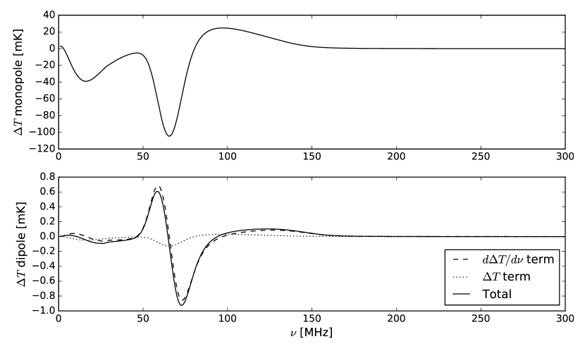
Figure 1: The figure showing the the EoR monopole and dipole. The monopole follows the model of Pritchard and Loeb (2010). Dipole has two terms, one proportional to the monopole and the other to its derivative in frequency direction. The latter dominates the signal.

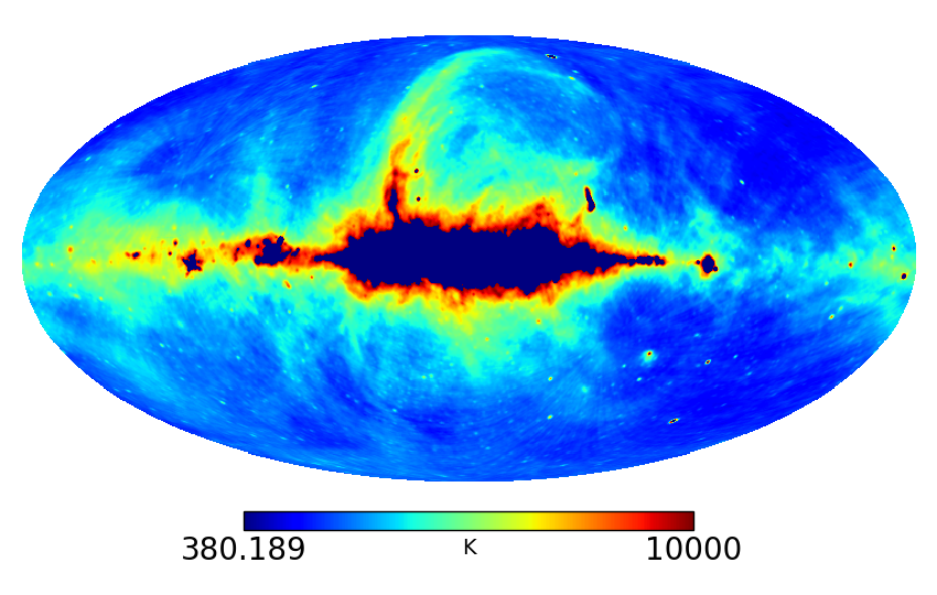
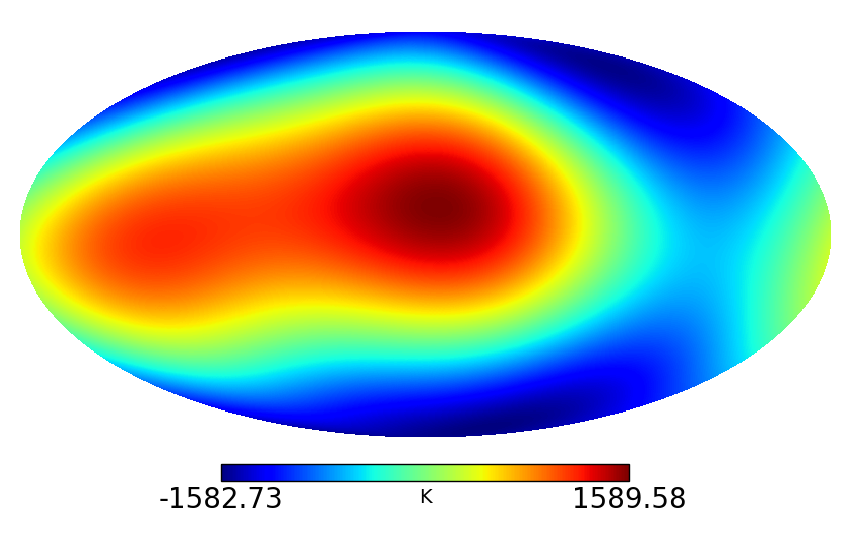
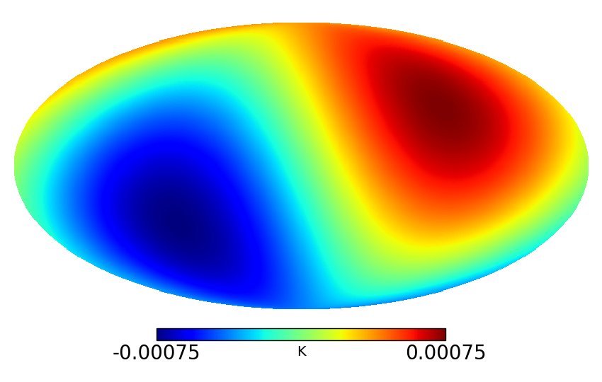
Figure 2: Estimated map of foregrounds at 60MHz using Global Sky Map de Oliveira-Costa et al. (2008) masked where it exceeds 10,000K (left), dipole and quadrupole of the above map (which are likely be confused for a finite sky covarage experiment (middle) and the map of the expected signal (right).

III The foreground question

The foregrounds, of course, are what is really difficult about these measurements. To give an impression of how difficult these can be, we plot a rough estimate of the foreground on Figure 2 at 60MHz. This figure is based on the Global Sky Models (GSM) from de Oliveira-Costa et al. (2008). We have masked pixels with temperature above $10^{4}$K, since an experiment with a finite angular resolution would be able to optimally downweight bright parts of the sky. The middle panel shows the dipole and quadrupole of the foreground while the right panel shows the estimated signal at the same frequency. We note that the constituent datasets that enter the GSM have uncertain fidelity on the largest scales and therefore the plotted foreground monopole and quadrupole might be significantly off.

Note that one such map exist at every frequency. While a search for monopole can marginalise over the foreground model while subtracting it, in dipole, the same marignalisation can be done subject to constraint that the resulting dipole is aligned with the cosmic dipole at every frequency. This is a very informative prior.

Methods for self-calibrated foreground rejection that rely on the fact that monopole does not vary across the sky, while the foregrounds doSwitzer and Liu (2014), can be easily generalised to dipole, since the dipole varies across the sky in a precisely known fashion.

IV What experiment would measure this

The most promising design the measuring this signal would be a differencing radiometer measuring the difference between two widely separated points on the sky. Unfortunately, unlike the CMB, where the signal above $\sim$ 1GHz is domimated by the CMB monopole, the foregrounds will dominate for EoR dipole measurement. This calls for a sufficient angular resolution to resolve the radio loud and radio quiet parts of the sky in order to allow optimal weighting Liu et al. (2013) and foreground rejection Switzer and Liu (2014). Moreover, radio-loud parts of the foreground sky can be used to characterise the frequency response of the receiver antenna.

The usual techniques used in CMB instrumentation could be used to inoculate against most common systematic: by putting the two receivers on a platform that rotates sufficiently fast, one can calibrate the beam differences between the two horns and by using 180^∘ hybridisation one can remove the receiver $1/f$ noise. Note that while variations of these techniques can be used in the monopole measurement, they are considerably less efficient. Since the noise will always be dominated by the sky noise there is no need for cryogenicaly cooled receivers.

What sensitivity would be required to perform this measurement? A convincing and accurate forecast would need to start with a mocked up radio-sky, including signal and realistic foregrounds, simulate observed maps with a realistic window function and then apply inverse covariance weighting to optimally extract the signal. This clearly exceeds the scope of this paper. Instead, we will make a back-of-the-envelope calculation to demonstrate that noise properties of a reasonable experiments can achieve desired statistical sensitivity.

We start with a radiometer equation that tells us that the error on measurement of the noise temperature is given by

$$\Delta T=\frac{T_{\rm sys}}{\sqrt{\Delta\nu t}},$$ (3)

where $T_{\rm sys}$ is the system temperature, $\Delta\nu$ is the observing bandwidth and $t$ is time to observe. Somewhat counter-intuitively, the receiving area does not come into this equation, since for a uniform unresolved radiation, the bigger collecting area is exactly canceled by a smaller beam-size. In our case we do want sufficient resolving power to be able to isolate radio-quiet and radio-loud parts of the foregrounds.

The radio sky at $60$MHz varies between $2,000$K and $40,000$K. From statistical perspective, one would just choose two quietest patches of the sky, however a scanning experiment does not have much freedom in choosing which parts of the sky to observe and besides more sky leads to better systematics control. But because we can still downweight radio-loud parts of the sky, it is not optimistic to assume just a uniform sky temperature of $10,000$K. At this level, the noise properties of receivers are irrelevant.

An experiment would measure the signal in many small frequency bins and the total signal to noise is given by an integral of observed bandwidth

$${\rm SNR}^{2}\sim\frac{N_{d}t}{2}\int_{\nu_{\rm min}}^{\nu_{\rm max}}\left(\frac{\Delta T_{\rm dip}(\nu)}{T_{\rm sys}(\nu)}\right)^{2}d\nu,$$ (4)

where $N_{d}$ is the number of receiving elements and the factor of 2 accounts for the fact that amplitude of the dipole accounts for maximum temperature difference, not typical one. Note that there could be extra factors of two, depending on the exact differencing scheme. Assuming an experiment operating between 50MHz and 100MHz, we find that 15 element radiometer could measure the signal at about $5\sigma$ over a course of a year. This result of course crucially (quadratically) depends on the assumed $T_{\rm sys}$. Assuming that weighting data optimally can bring the effective temperature to $5000$K, only four elements would sufficeLiu et al. (2013).

V Discussion & Conclusions

Differencing has proven to be one of the most successful paradigms in the experimental physics: differential measurements are easy, absolute measurements are hard. We apply this principle to the problem of measuring the EoR monopole. Due to our motion with respect to the cosmic rest frame, this signal is modulated in a dipole fashion. The amplitude of this dipole is supressed but somewhat less than $v_{d}/c$ factor due to a non-trivial frequency structure of the signal. This supression of the signal could be more than compensated by considerably easier systematic control in the dipole measurement:

• The direction of the CMB dipole is know very well and more importantly, the galactic foreground will have both a different true dipole and the doppler dipole of the foregrounds will be different: motion of the solar system with respect to the CMB is not the same as its motion with respect to the galaxy. This can be used to estimate the residual foreground contamination.

• The standard differencing techniques well known in the radio astronomy can be used to great advantage in this set up. This should help in dealing with radio frequency interference, the amplifier $1/f$ noise and the earth’s atmosphere. However, the mean beam chromaticity will remain a significant issue.

• The signal derived in this way could be used to cross-check measurements derived from the monopole, since the information content is the same. In fact, one could imagine an experiment that would measure both at the same time.

• Since the signal is proportional to the derivative of the monopole with respect to the frequency, this technique could be potentially very efficient for reionization scenarios that happen rapidly.

We have made a back-of-the-envelope estimate of the require signal-to-noise and determined that signal is in principle measurable in a reasonable amount of time for a reasonable experiment. We hope that this warrants a more accurate forecasts, which would take into account the spactial and frequency variation of foregrounds and work out an optimal map-making scheme.

References

- Furlanetto et al. (2006) S. R. Furlanetto, S. P. Oh, and F. H. Briggs, Phys. Rept. 433, 181 (2006), arXiv:astro-ph/0608032 .
- Morales and Wyithe (2010) M. F. Morales and J. S. B. Wyithe, Annu. Rev. Astro. Astrophys. 48, 127 (2010), arXiv:0910.3010v1 .
- Pritchard and Loeb (2012) J. R. Pritchard and A. Loeb, Rep. Prog. Phys. 75, 086901 (2012), arXiv:1109.6012v2 .
- Liu et al. (2016) A. Liu, J. R. Pritchard, R. Allison, A. R. Parsons, U. Seljak, and B. D. Sherwin, Phys. Rev. D 93 (2016), arXiv:1509.08463v2 .
- Tingay et al. (2012) S. J. Tingay, R. Goeke, J. N. Hewitt, E. Morgan, R. A. Remillard, C. L. Williams, J. D. Bowman, D. Emrich, S. M. Ord, T. Booler, B. Crosse, D. Pallot, W. Arcus, T. Colegate, P. J. Hall, D. Herne, M. J. Lynch, F. Schlagenhaufer, S. Tremblay, R. B. Wayth, M. Waterson, D. A. Mitchell, R. J. Sault, R. L. Webster, J. S. B. Wyithe, M. F. Morales, B. J. Hazelton, A. Wicenec, A. Williams, D. Barnes, G. Bernardi, L. J. Greenhill, J. C. Kasper, F. Briggs, B. McKinley, J. D. Bunton, L. deSouza, R. Koenig, J. Pathikulangara, J. Stevens, R. J. Cappallo, B. E. Corey, B. B. Kincaid, E. Kratzenberg, C. J. Lonsdale, S. R. McWhirter, A. E. E. Rogers, J. E. Salah, A. R. Whitney, A. Deshpande, T. Prabu, A. Roshi, N. Udaya-Shankar, K. S. Srivani, R. Subrahmanyan, B. M. Gaensler, M. Johnston-Hollitt, D. L. Kaplan, and D. Oberoi, (2012), arXiv:1212.1327v1 .
- Parsons et al. (2010) A. R. Parsons, D. C. Backer, R. F. Bradley, J. E. Aguirre, E. E. Benoit, C. L. Carilli, G. S. Foster, N. E. Gugliucci, D. Herne, D. C. Jacobs, M. J. Lynch, J. R. Manley, C. R. Parashare, D. J. Werthimer, and M. C. H. Wright, The Astronomical Journal 139, 1468 (2010), arXiv:0904.2334v2 .
- Rottgering et al. (2006) H. J. A. Rottgering, R. Braun, P. D. Barthel, M. P. van Haarlem, G. K. Miley, R. Morganti, I. Snellen, H. Falcke, A. G. de Bruyn, R. B. Stappers, W. H. W. M. Boland, H. R. Butcher, E. J. de Geus, L. Koopmans, R. Fender, J. Kuijpers, R. T. Schilizzi, C. Vogt, R. A. M. J. Wijers, M. Wise, W. N. Brouw, J. P. Hamaker, J. E. Noordam, T. Oosterloo, L. Bahren, M. A. Brentjens, S. J. Wijnholds, J. D. Bregman, W. A. van Cappellen, A. W. Gunst, G. W. Kant, J. Reitsma, K. van der Schaaf, and C. M. de Vos, (2006), arXiv:astro-ph/0610596v2 .
- Paciga et al. (2013) G. Paciga, J. G. Albert, K. Bandura, T.-C. Chang, Y. Gupta, C. Hirata, J. Odegova, U.-L. Pen, J. B. Peterson, J. Roy, R. Shaw, K. Sigurdson, and T. Voytek, Monthly Notices of the Royal Astronomical Society 433, 639 (2013), arXiv:1301.5906v2 .
- Monsalve et al. (2016) R. A. Monsalve, A. E. E. Rogers, J. D. Bowman, and T. J. Mozdzen, (2016), arXiv:1602.08065v1 .
- Ellingson et al. (2013) S. W. Ellingson, G. B. Taylor, J. Craig, J. Hartman, J. Dowell, C. N. Wolfe, T. E. Clarke, B. C. Hicks, N. E. Kassim, P. S. Ray, L. J. Rickard, F. K. Schinzel, and K. W. Weiler, IEEE Trans. Antennas Propagat. 61, 2540 (2013), arXiv:1204.4816v3 .
- Greenhill and Bernardi (2012) L. J. Greenhill and G. Bernardi, (2012), arXiv:1201.1700v1 .
- Wouthuysen (1952) S. A. Wouthuysen, AJ 57, 31 (1952).
- Field (1958) G. B. Field, Proceedings of the IRE 46, 240 (1958).
- Pritchard and Loeb (2010) J. R. Pritchard and A. Loeb, Phys. Rev. D 82 (2010), arXiv:1005.4057v1 .
- de Oliveira-Costa et al. (2008) A. de Oliveira-Costa, M. Tegmark, B. M. Gaensler, J. Jonas, T. L. Landecker, and P. Reich, Mon. Not. Roy. Astron. Soc. 388, 247 (2008), arXiv:0802.1525 .
- Switzer and Liu (2014) E. R. Switzer and A. Liu, Astrophys. J. 793, 102 (2014), arXiv:1404.7561 .
- Liu et al. (2013) A. Liu, J. R. Pritchard, M. Tegmark, and A. Loeb, Phys. Rev. D 87 (2013), arXiv:1211.3743v3 .