Many-body methods in agent-based epidemic models

Abstract

The susceptible-infected-susceptible (SIS) agent-based model is usually employed in the investigation of epidemics. The model describes a Markov process for a single communicable disease among susceptible (S) and infected (I) agents. However, the disease spreading forecasting is often restricted to numerical simulations, while analytic formulations lack both general results and perturbative approaches since they are subjected to asymmetric time generators. Here, we discuss perturbation theory, approximations and application of many-body techniques in epidemic models in the framework for squared norm of probability vector $|P(t)|^{2}$, in which asymmetric time generators are replaced by their symmetric counterparts.

Proper planning and management lie in the foundation of efficient health and sanitary policies Team (2016). The decision-making process usually relies on predictions from epidemic models and raw data to rule the best available policy to mitigate the disease spreading. Resource planning becomes even more relevant during the emergence of new communicable diseases, as improper actions may extend the duration or adversely impact health workers Heesterbeek et al. (2015). Despite the success attained by traditional epidemic models for large scale epidemics in the past, they have been unable to produce reliable predictions for small scale disease spreading in heterogeneous populations Heesterbeek et al. (2015); Bansal et al. (2007); Eames and Keeling (2002). This issue is further enhanced due to the stochastic nature of pathogen transmission mechanisms and patient care. As such, a considerable amount of epidemic models have been proposed to mimic the correct behavior for spreading of communicable infectious diseases.

The simplest susceptible-infected-susceptible (SIS) model considers the time evolution of a single communicable disease among $N$ susceptible (S) and infected (I) agents Pastor-Satorras et al. (2015). The infected agents may either transmit the disease to susceptible agents with constant probability $\alpha$, turning them into infected agents $S\rightarrow I$, or undergo the recovery process $I\rightarrow S$ with probability rate $\beta$, during a fixed time interval $\delta t$. Furthermore, two approaches are available to describe the disease spreading in the SIS model for a fixed population of size $N$: compartmental and stochastic. In the compartmental approach relevant quantities are well-described by averages Keeling and Eames (2005), from which one derives non-linear differential equations. For instance, the number of infected agents $n(t)$, for fixed $N$, in the compartmental SIS model is

$$\frac{dn}{dt}=\tilde{\alpha}n\left(1-\frac{n}{N}\right)-\tilde{\beta}n.$$ (1)

This is the expected behavior for large homogeneous populations, where fluctuations are negligible. Introduction of effective transmission ($\tilde{\alpha}$) and recovery ($\tilde{\beta}$) probabilities rates contemplates effects due to heterogeneous population. This parameter estimations employ networks, with size $N$, as substrate to display the varying degree of non-uniformity within a population. In this scheme, each vertex in the network contains a single agent, while the links among agents are given by the corresponding adjacency matrix $A$. Thus, non-trivial topological aspects of $A$ are incorporated in the effective transmission and cure rates Bansal et al. (2007); Eames and Keeling (2002); Pastor-Satorras et al. (2015); Keeling and Eames (2005); Pastor-Satorras and Vespignani (2001).

The stochastic approach also requires networks to describe the population heterogeneity. However, contrary to the compartmental approach, the assumption about negligible fluctuations is removed, meaning averages alone are not sufficient to properly describe the disease spreading. In fact, fluctuations are intrinsic components in stochastic formulations and their relevance increases with vanishing $N$ van Kampen (1992), a much more realistic scenario in modeling emergence of small scale epidemics of communicable infectious diseases Heesterbeek et al. (2015). In this approach, transition probabilities among configurations of $N$ agents are expressed by the transition matrix $\hat{T}$, and take place during the time interval $\delta t$ Reichl (1998); Alcaraz et al. (1994); Alcaraz and Rittenberg (2008). The disease transmission and agent recovery are modeled as probability vector $|P(t)\rangle$ of a Markov process with time interval $\delta t$ taken to be small enough so that only one recovery or one transmission event takes place in the entire population. This is compatible with the Poissonian assumption Pastor-Satorras et al. (2015).

As a closing remark, one notices the transition matrix is analogous to the time evolution operator in quantum theories. As a result, the eigenvalues and eigenvectors of $\hat{T}$ express the time evolution of agent-configurations. Despite the striking similarity between both operators, $\hat{T}$ is often asymmetric, restraining its use to small values of $N$ for epidemic models in numerical simulations or introducing severe obstacles for analytic solutions. These issues hinder the systematic development of perturbation theories for agent-based epidemic models, often requiring fresh simulations to forecast the impact of small variations of the parameters of the model, contrary to the rationale behind perturbation theory.

Here, we first briefly review results Nakamura et al. (2016) derived from the squared norm of the probability vector $|P(t)|^{2}$. The formalism proposed therein allow us to further explore the operatorial content of the corresponding Markov process. More specifically, we demonstrate the time evolution is also achieved in a framework that only requires eigenvalues derived from Hermitian operators. This leads to a constrained multivariate equation, which can be solved by standard optimization techniques. We explore the fact the time evolution heavily relies on the eigendecomposition and formulate perturbative corrections to epidemic models. Additionally, we also discuss methods usually employed in quantum many-body problems and Statistical Physics, such as the the Bethe-Peierls approximation Bethe (1935) and the Holstein-Primakoff transformations Holstein and Primakoff (1940); Emary and Brandes (2003a, b).

I SIS model

One of the key aspect of agent-based models is the use of networks to describe heterogeneity among the distinct agents Eames and Keeling (2002); Keeling and Eames (2005); Bansal et al. (2007); Pastor-Satorras et al. (2015), as Fig. 1 depicts. By taking into account the individuality of each agent, the web of connections between them creates disease spreading patterns, due to the development of characteristic pathogen mobility within the underlying population. Epidemic time duration is shorter for populations consisting of loose connected agents, whereas the potential of disease dissemination is expected to be stronger for hub-like agents.

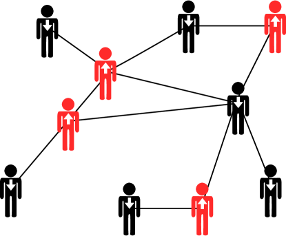
Figure 1: Networks are used to reproduce the heterogeneous interactions in a population formed by susceptible ($\downarrow$, black) and infected agents ($\uparrow$, red). The topology of the network figures among the relevant factors that impact the disease spreading.

Networks are characterized by their topological quantities such as degree, connectivity, centrality, etc., and we label the collection of these descriptive quantities as $\omega$. As long as they share the same set of topological characteristic values $\omega$, several distinct objects may in fact represent the same network $\mathcal{N}(\omega)$. Graphs are natural candidates to represent networks Albert and Barabási (2002) since they are mathematical constructions formed by interconnected vertices $V_{k}$ ($k=0,\ldots,N-1$). For each graph, the adjacency matrix $A$ ($N\times N$) describes all present connections among vertices; the matrix elements are $A_{ij}=1$, if vertices $i$ and $j$ are connected or vanish otherwise. In this context, an ensemble of graphs is a convenient way to represent a network, i.e., one graph $G(\omega)$ is a single realization of the network $N(\omega)$, whose set of topological quantities are $\omega$.

The correspondence between networks and agent-based models requires that each vertex contains exactly one agent, which state belongs a discrete domain. More precisely, $V_{k}$ holds the discrete state $k$-th agent and $A$ reproduce the connection among agents. Once agents and their interconnections are properly written, we address the $N$-agent configuration health state. Let the current health status of the $k$-th agent be $\sigma_{k}$, which for may acquire two values, namely, $\sigma_{k}=\downarrow$ (susceptible) or $\sigma_{k}=\uparrow$ (infected). The vector

$$\lvert C_{\mu}\rangle\equiv\lvert\sigma_{1}\sigma_{2}\cdots\sigma_{N}\rangle,$$ (2)

with $\mu=0,1,\ldots,2^{N}-1$, describes the health status configuration of $N$ agent. Since there are two health states available per agent, the total number of distinct configurations is $2^{N}$. We enumerate each configuration $C_{\mu}$ using binary arithmetic:

$$\mu=\delta_{\sigma_{0},\uparrow}2^{0}+\delta_{\sigma_{1},\uparrow}2^{1}+\cdots+\delta_{\sigma_{N-1},\uparrow}2^{N-1}.$$ (3)

For instance, the configuration containing only healthy individuals is $\lvert C_{0}\rangle=\lvert\downarrow\downarrow\downarrow\cdots\downarrow\rangle$, whereas the configuration where only the $k=1$ agent is infected is $\lvert C_{2}\rangle=\lvert\downarrow\uparrow\downarrow\cdots\downarrow\rangle$. Henceforth, we set the following notation: Latin integer indices run over agents $[0,N-1]$, while Greek integer indices enumerate configurations $[0,2^{N}-1]$.

The set formed by configurations $\{C_{\mu}\}$ spans the finite vector space $\mathbbm{H}$. Within $\mathbbm{H}$, one may define the relevant operators for epidemic spreading. The operator $\hat{\sigma}^{z}_{k}$ shows whether the $k$-th agent is infected ($\uparrow$) or not ($\downarrow$), namely,

$$\hat{\sigma}^{z}_{k}|\sigma_{1}\sigma_{2}\cdots\sigma_{N}\rangle=(\delta_{\sigma_{k}\uparrow}-\delta_{\sigma_{k}\downarrow})|\sigma_{1}\sigma_{2}\cdots\sigma_{N}\rangle.$$ (4)

The number of infected agents at vertex $k$ is obtained via the operator

$${\hat{n}_{k}=\frac{1}{2}\;(\hat{\sigma}^{z}_{k}+1)}\;,$$ (5)

while the total number of infected agents in the population is

$$\hat{n}=\frac{1}{2}\sum_{k=0}^{N-1}\hat{\sigma}^{z}_{k}+\frac{N}{2}.$$ (6)

Agent health status are flipped by the action of $\hat{\sigma}_{k}^{+}$ and $\hat{\sigma}_{k}^{-}$:

$$\hat{\sigma}_{k}^{+}\lvert\sigma_{1}\cdots\downarrow_{k}\cdots\sigma_{N}\rangle= \lvert\sigma_{1}\cdots\uparrow_{k}\cdots\sigma_{N}\rangle,$$ (7)

$$\hat{\sigma}_{k}^{-}\lvert\sigma_{1}\cdots\uparrow_{k}\cdots\sigma_{N}\rangle= \lvert\sigma_{1}\cdots\downarrow_{k}\cdots\sigma_{N}\rangle,$$ (8)

null otherwise. They are combined to form another $\hat{\sigma}_{k}^{x}=\hat{\sigma}_{k}^{+}+\hat{\sigma}_{k}^{-}$. The localized operators $\hat{\sigma}_{k}^{\pm}$ and $\hat{\sigma}_{k}^{z}$ satisfy well-known algebraic relations. For each $k$, $\hat{\sigma}_{k}^{\pm,z}$ form local $\textrm{su}(2)$ algebra, with the following structure constants: $[\hat{\sigma}_{k}^{z},\hat{\sigma}_{k}^{\pm}]=\pm 2\hat{\sigma}_{k}^{\pm}$ and $[\hat{\sigma}_{k}^{+},\hat{\sigma}_{k}^{-}]=\sigma_{k}^{z}$. However, they also exhibit local fermionic anticommutation rules, $\{\hat{\sigma}_{k}^{+},\hat{\sigma}_{k}^{-}\}=1$, and non-local bosonic relations, $[\hat{\sigma}_{k}^{r},\hat{\sigma}_{k^{\prime}}^{s}]=0$, for $k\neq k^{\prime}$ and $r,s=\pm,z$. The dual fermionic-bosonic behavior is a familiar occurrence in quantum spinchains Alcaraz et al. (1988); Nakamura et al. (2016). Usually, it is advisable to select either the fermionic behavior via the Jordan-Wigner transformation Batista and Ortiz (2001) or, alternatively, the bosonic behavior via the Holstein-Primakoff transformation Holstein and Primakoff (1940). We postpone the behavior-selection as our intention in this section concerns general aspects.

For any Markov process, the probability vector represents the system and is written as

$$\lvert P(t)\rangle=\sum_{\mu}P_{\mu}(t)\lvert C_{\mu}\rangle\;,$$ (9)

where $P_{\mu}(t)$ is the probability to find $N$ agents in the configuration $\lvert C_{\mu}\rangle$, at time $t$, subjected to probability conservation constraint,

$$\sum_{\mu}P_{\mu}(t)=1.$$ (10)

Another integral part of the Markov process is the transition matrix $\hat{T}$, which weight transitions among configurations in a fixed time interval $\delta t$, creating the temporal succession:

$$\lvert P(t+\delta t)\rangle=\hat{T}\lvert P(t)\rangle.$$ (11)

The details concerning disease transmission or recovery in epidemic model are included in $\hat{T}$ by considering operators that act over the $N$-agent configurations $\lvert C_{\mu}\rangle$. In the SIS model, an infected agent at vertex $k$ is subjected to three distinct outcomes after the action of $\hat{T}$: transmit the disease to a susceptible connected agent; recover to the susceptible state; or remain unchanged.

The recovery event for the $k$-th agent is executed by the operator $\hat{\sigma}^{-}_{k}\hat{n}_{k}$. Brief inspection shows the action is quite simple: if the $k$-th agent is currently infected, the health status flips to susceptible. On contrary, if the $k$-th agent is susceptible, it returns the null vector. Although the recovery event does not involve the underlying network, the disease transmission event does. As a result, the corresponding operator $A_{km}\hat{\sigma}^{+}_{m}\hat{n}_{k}$ transmits the disease from the $k$-th agent to $m$-th agent. Similarly to the recovery process, the operator $\hat{n}_{k}$ only checks whether the $k$-th agent is infected. The difference appears due to the adjacency matrix $A_{mk}$ and the infection operator $\hat{\sigma}^{+}_{m}$. Note that if the $m$-th agent is already infected, the operatorial action returns the null vector as well. Finally, the event to remain unchanged requires diagonal operators and accounts for all the other possible non-diagonal events. The operator which provides the number of available outcomes of disease transmission for $k$-th agent is $\sum_{j}A_{jk}(1-\hat{n}_{j})\hat{n}_{k}$; whereas the operator that accounts for the chance to not recover is simply $\hat{n}_{k}$.

Under the Poissonian assumption, one only considers a single recovery or a single infection event, per time interval $\delta t$. Under this circumstances, the transition matrix reads

$$\hat{T}=\mathbbm{1}-\frac{\alpha}{N}\sum_{kj}\left[A_{jk}(1-\hat{n}_{j}-\hat{\sigma}^{+}_{j})+\Gamma\delta_{kj}(1-\hat{\sigma}^{-}_{j})\right]\hat{n}_{k},$$ (12)

with $\Gamma=\beta N/\alpha$. The diagonal components are the probabilities for the configuration to remain unchanged after one time step. Disease spreading explicitly carries the network topology due to the contribution of $A$. More importantly, the transition matrix $\hat{T}$ contains non-Hermitian operators and, hence, its left and right eigenvectors, $\langle\chi_{\mu}\rvert$ and $\lvert\phi_{\mu}\rangle$, respectively, are not related by Hermitian transposition.

We emphasize that the construction of Eq. (12) considers only a single graph. In general, agent-based models are built under the hypothesis of $N\gg 1$. The reasoning behind this choice lies in the network averaging process. If the graph is large enough $N\gg 1$, one expects to recover the network topological quantities $\omega$ within a single realization. This statement is the equivalent to the ergodic hypothesis, where the ensemble average over $M$ graphs is replaced by the average within a single graph (self-averaging/annealing case). This expectation is reasonable but cannot hold for moderate $N$. In what follows, we explicitly consider the network ensemble containing $M>1$ graphs (quenched). For that purpose, let $G_{i}\in\{G_{0},G_{1}\ldots,G_{M-1}\}$ be the $i$-th graph in the network ensemble. Furthermore, for each graph $G_{i}$ there is a corresponding adjacency matrix $A^{i}$. For fixed initial condition, Eq. (11) tells us the time evolution is a linear transformation so the average over the network ensemble is estimated by $\hat{\bar{T}}=M^{-1}\sum_{i}\hat{T}^{(i)}$, where $\hat{T}^{(i)}$ is the transition matrix using the graph $G_{i}$ ($i=0,1,\dots,M-1$). For the SIS model, the averaging process is tracked down to

$$\bar{A}_{jk}=\frac{1}{M}\sum_{l=0}^{M-1}A_{jk}^{(l)},$$ (13)

with $A^{(l)}$ corresponding to the adjacency matrix of $G_{l}$ and the bar symbol represents the ensemble average. Notice that $\bar{A}_{jk}$ is not restricted to the integers 0 or 1 any longer. In practice, Eq. (13) claims the estimator $\bar{A}$ is a real $N\times N$ matrix and we can safely drop to bar symbol. However, sudden changes in the network topological properties $\omega$ must be investigated using Eq. (13), from which one derives perturbative operators.

Since $\hat{T}$ in Eq. (12) is time independent, the Taylor expansion of Eq. (11) leads to the following system of differential equations:

$$\frac{dP_{\mu}}{dt}=-\sum_{\nu}H_{\mu\nu}P_{\nu}(t),$$ (14)

where $H_{\mu\nu}$ are the matrix elements of the time generator

$${\hat{H}\equiv\frac{\mathbbm{1}-\hat{T}}{\delta t}}\;.$$ (15)

The operator $\hat{H}$ governs the dynamics of disease spreading and whose normal modes are labeled after the eigenvalues $\{\lambda_{\mu}\}$. The formal solution to Eq. (14) is

$$\lvert P(t)\rangle=\mathrm{e}^{-\hat{H}t}\lvert P(0)\rangle.$$ (16)

Clearly, the eigenvalues must satisfy $\lambda_{\mu}\geq 0$, for any $\mu$, vanishing only for stationary states Reichl (1998). In addition, the corresponding spectral density function $\rho(\lambda)$ depends on the couplings present in Eq. (12), namely, the disease transmission and recovery probabilities as well as the network average adjacency matrix $A$.

II Theoretical approach

One of the main goals in epidemic models is the development of methods to predict the way epidemics change when parameters are subjected to small variations. If such predictions are robust, preemptive actions to lessen the epidemic are also expected to achieve better results. In physical theories, small changes in couplings or substrate are often investigated under perturbative schemes based on simpler models, which often have known orthonormal modes. In epidemic models, however, one must work with asymmetric operators $\hat{H}$ and their left and right eigenvectors in Eq. (16). Despite the complexities related to the operatorial content of $\hat{H}$, the stochastic nature of the problem ensures the conservation of total probability $\sum_{\mu}P_{\mu}(t)=1$ for any $t$. Another relevant descriptive variable derived from $\lvert P(t)\rangle$ is the squared norm,

$$\lvert P(t)\rvert^{2}=\langle P(t)|P(t)\rangle=\sum_{\mu=0}^{2^{N}-1}P_{\mu}(t)^{2}.$$ (17)

As noted in Ref. Nakamura et al. (2016), probability conservation does not enforce conservation of $\lvert P(t)\rvert^{2}$ along time, occurring only after the system reaches complete stationarity. Therefore, $\lvert P(t)\rvert^{2}$ may be used to assess general properties of the stochastic model during both transient and stationary phases.

Since the squared norm can only assume values in the interval $[0,1]$, one may consider a single differential equation to investigate the time evolution of $\lvert P(t)\rvert^{2}$. Taking the time derivative of Eq. (17) and using Eq. (14) results in

$$-\frac{d}{dt}|P(t)|^{2}=2\langle P(t)\rvert\hat{\mathcal{H}}\lvert P(t)\rangle.$$ (18)

Unlike $\hat{H}$, the symmetrized time generator

$${\hat{\mathcal{H}}\equiv\frac{\hat{H}^{T}+\hat{H}}{2}}$$ (19)

is Hermitian with orthonormal basis $\{\lvert\psi_{\mu}\rangle\}$ and corresponding eigenvalues $\{\Lambda_{\mu}\}$, for $\mu=0,\ldots,2^{N}-1$. The eigenvalues $\Lambda_{\mu}$ differ from their counterparts $\lambda_{\mu}$, since $\Lambda_{\mu}$ are not positive semi-definite, while the complex coefficients

$$\pi_{\mu}(t)\equiv\langle\psi_{\mu}|P(t)\rangle$$ (20)

are not probabilities, even though they are used to evaluate the configurational probabilities

$$P_{\mu}(t)=\sum_{\nu}\langle C_{\mu}|\psi_{\nu}\rangle\,\pi_{\nu}(t).$$ (21)

Figure 2 illustrates the time evolution of $\lvert P(t)\rvert^{2}$ for arbitrary Markov process.

Figure 2: Time evolution of $\lvert P(t)\rvert^{2}$ for arbitrary Markov process. The system starts at $t=t_{0}$ with initial condition $P_{\mu}(t_{0})=\delta_{\mu\xi}$. During the transient phase, the number of available configurations increases, lowering the value of $\lvert P(t)\rvert^{2}$. At $t=t_{c}$, $\lvert P(t_{c})\rvert^{2}$ develops a minimum. As the system continues to evolve, the squared norm continuously increases until stationarity is achieved. In this particular illustration, the number of stationary states is larger than unity, producing $\lim_{t\rightarrow\infty}\lvert P(t)\rvert^{2}<1$.

The spectral decomposition of $\lvert P(t)\rangle=\sum_{\mu}\pi_{\mu}(t)\lvert\psi_{\mu}\rangle$ in Eq. (18) produces:

$$\sum_{\mu}\left(\frac{1}{2}\frac{d}{dt}+\Lambda_{\mu}\right)\lvert\pi_{\mu}(t)\rvert^{2}=0,$$ (22)

subjected to the constraint $\sum_{\mu\nu}\langle C_{\mu}|\psi_{\nu}\rangle\pi_{\nu}(t)=1$. Notice that Eq. (22) is valid for any time instant $t$. As such, one may also integrates the expression in Eq. (22) taking into account the probability constraint with help of one Lagrange multiplier $h$,

$$\mathcal{S}_{0} \equiv\sum_{\mu}\int_{t_{0}}^{t_{f}}dt\left[\frac{1}{2}\frac{d}{dt}\lvert\pi_{\mu}\rvert^{2}+\Lambda_{\mu}\lvert\pi_{\mu}\rvert^{2}\right],$$ (23)

$$\mathcal{S} \equiv S_{0}+h\sum_{\mu\nu}\int_{t_{0}}^{t_{f}}dt\left[\frac{\pi_{\nu}}{2}\langle C_{\mu}|\psi_{\nu}\rangle+\frac{\pi_{\nu}^{*}}{2}\langle\psi_{\nu}|C_{\mu}\rangle-1\right],$$ (24)

where $t_{0}$ and $t_{f}$ are the fixed initial and final time instants, respectively. Equations (23) and (24) share striking similarity with the classical action of Mechanics Goldstein (1950). Since we are only interested in stationarity and extrema states so we can neglect Eqs. (23-24) for now. In fact, the condition of vanishing derivative in Eq. (22) results in the following algebraic equation:

$$\sum_{\mu}|\tilde{\pi}_{\mu}|^{2}\Lambda_{\mu}=0,$$ (25)

where $\tilde{\pi}_{\mu}$ either are the coefficients corresponding to stationary states or local extrema.

Formally, Eq. (25) may be solved using optimization algorithms for constrained quadratic problems. Of course, $2^{N}$ optimization problems are still formidable numerical problems and also involves the numerical approach taken for each optimization algorithm as well. Failure to converge to correct solutions or only walk in a particular neighborhood in the solution space are among common sources of problems. Furthermore, the derivation of Eqs. (22) and (25) assumes the eigenvalues $\{\Lambda_{\mu}\}$ and the corresponding eigenvectors $\{\psi_{\mu}\}$ are known, which again may be a complex $2^{N}$ diagonalization problem depending on the algebraic form of $\hat{\mathcal{H}}$.

However, the aforementioned hardships are the crucial aspects one must consider to decide whether to use Eqs. (22) and (25) or Eq. (14). The answer is very simple: $\lvert P(t)\rvert^{2}$ is only useful if symmetries are present in $\hat{\mathcal{H}}$ but not in $\hat{H}$ Nakamura et al. (2016). Additional symmetries simplify the diagonalization problem and also introduce explicit bounds in root-finding procedures. It is easy to find examples where such symmetry increase occurs. For instance, consider $\hat{H}=\hat{\sigma}^{+}_{1}+\hat{\sigma}^{+}_{2}$ so that the corresponding Hermitian generator is $\hat{\mathcal{H}}=\sigma^{x}_{1}+\sigma^{x}_{2}$, whose eigenvectors are grouped according to the quantum number $m_{x}=-1,0,1$. Therefore, if additional symmetries are available for $\hat{\mathcal{H}}$, traditional optimization algorithms become valuable resources to solve Eq. (25) and, thus, the stationary states of Markov processes and their corresponding occurrence probabilities.

As a practical example to verify the results in Eq. (25), consider the SIS model with $N=3$ agents and $\alpha=N/10$ and $\Gamma=0$, in the fully connected network $A_{ij}=(1-\delta_{ij})$. This set of parameters and network topology reproduce the SI model. From Eqs. (12) and (15), the Hermitian time generator for the SIS model is

$$\hat{\mathcal{H}}_{\textrm{SIS}}= \hat{\mathcal{H}}_{0}+\hat{\mathcal{H}}_{1}\;,$$ (26)

$$\hat{\mathcal{H}}_{0}= +\frac{\alpha}{N}\sum_{kj}\left[A_{jk}(1-\hat{n}_{j})+\Gamma\delta_{kj}\right]\hat{n}_{k},$$ (27)

$$\hat{\mathcal{H}}_{1}= -\frac{\alpha}{2N}\sum_{kj}\left[A_{jk}({\hat{\sigma}_{j}^{+}\hat{n}_{k}+\hat{n}_{k}\hat{\sigma}^{-}_{j}})+{\Gamma}\delta_{kj}\hat{\sigma}_{k}^{x}\right].$$ (28)

In this case, there are four eigenvalues of $\hat{\mathcal{H}}_{\textrm{SIS}}$ relevant to the description of stationary states, namely, $\Lambda_{0}=0$, $\Lambda_{3}=0.1571993$, $\Lambda_{6}=0.3514137$ and $\Lambda_{7}=-0.1086130$. The trivial stationary state (none infected) is obtained setting $\tilde{\pi}_{\mu}=\delta_{\mu 0}$. The stationary state where all agents are infected is obtained using $\tilde{\pi}_{3}=0.3977703$, $\tilde{\pi}_{6}=-0.3803660$ and $\tilde{\pi}_{7}=0.8349255$.

III Perturbative methods and approximations

The ability to predict causal effects in the disease spreading is surely desirable for any epidemic model, as it allows decision-makers to select adequate strategies to mitigate new incidence cases and funding priorities. Among them, effects caused by small perturbations in the underlying contact network are specially important for agent-based models. As Ref. Pastor-Satorras et al. (2015) states, heterogeneous population hinders analytical insights about perturbative effects. Nonetheless, Eq. (25) provides an alternative way to introduce perturbative methods and approximations to epidemic models, since it relies on the Hermitian generator $\hat{\mathcal{H}}$. This is relevant because the standard time independent perturbation theory may be used to evaluate corrections to the quantities relevant to Eq. (25), namely, the eigenvalues $\Lambda_{\mu}$ and the coefficients $\tilde{\pi}_{\mu}$.

For the sake of clarity, we consider a finite number of topological values $\omega_{r}$ ($r=1,\ldots,R$) to characterize the network. In this context, a simple perturbative scheme is attained by considering the change $\omega_{r}\rightarrow\omega_{r}+\delta\omega_{r}$, with $|\delta\omega_{r}|\leq\delta\omega$ for any $r=1,2,\ldots,R$ and fixed $\delta\omega\ll 1$. The quantities $\omega_{r}$ are expected to be complicated functions so that the variations $\delta\omega_{r}$ are not completely independent. Nonetheless, they are still calculated from estimators derived from the average adjacency matrix $\bar{A}$. Therefore, one expects a corresponding perturbative matrix $\delta\omega B$ to be added to the average adjacency matrix:

$$\bar{A}_{ij}\rightarrow\bar{A}_{ij}+\delta\omega B_{ij}.$$ (29)

The details of the matrix representation $B$ are specific for each perturbation set $\{\omega_{r}\}$ adopted, but the relevant information lies in the coupling $\delta\omega$, as it provides a natural perturbative parameter. Now, it is a simple task to identify the perturbation $\hat{V}$ in the time generator,

$$\hat{\mathcal{H}} =\hat{\mathcal{H}}_{0}+\hat{\mathcal{H}}_{1}+\delta\omega\,\hat{V},$$ (30)

$$\hat{V} =\frac{\alpha}{2N}\sum_{kj}B_{jk}\left[2(1-\hat{n}_{j})\hat{n}_{k}-\hat{\sigma}_{j}^{+}\hat{n}_{k}-\hat{n}_{k}\hat{\sigma}_{j}^{-}\right].$$ (31)

A few selected cases merit further attention. First, the special case $B=zA$, with $\delta\omega z\in[-1,1]$, recovers the effective coupling formulation $\alpha\rightarrow\alpha(1+z\delta\omega)$ in random networks. Another interesting case occurs if $A$ and $B$ are periodic regular networks with distinct periods, $t_{A}\neq t_{B}$, respectively. Depending on the initial condition and the ratio $t_{B}/t_{A}$, the perturbation $\hat{V}$ may either connect all available states, or lock the time evolution in a periodic cycle.

Hermiticity is sufficient to warrant Rayleigh-Schrödinger perturbation theory and produces first order corrections to eigenvalues and eigenvectors, respectively,

$$\Lambda_{\mu}^{(1)} =\langle\psi_{\mu}|\hat{V}|\psi_{\mu}\rangle,$$ (32)

$$\tilde{\pi}_{\mu}^{(1)} =\sideset{}{{}^{\prime}}{\sum}_{\nu}\frac{\lvert\langle\psi_{\mu}|\hat{V}|\psi_{\nu}\rangle\rvert^{2}}{\Lambda_{\nu}-\Lambda_{\mu}}.$$ (33)

The prime indicates the sum excludes degenerate states with eigenvalue $\Lambda_{\mu}$. Substituting these results into Eq. (25) and discarding second order corrections, one arrives at

$$\sum_{\mu}\left[2\Lambda_{\mu}\textrm{Re}(\tilde{\pi}_{\mu}\tilde{\pi}_{\mu}^{(1)})+\lvert\tilde{\pi}_{\mu}\lvert^{2}\Lambda_{\mu}^{(1)}\right]=0.$$ (34)

While the perturbative corrections are given by Eqs. (32) and (33), the relation in Eq. (34) shows they might not be independent. Similarly, the perturbative corrections for configurational probabilities $P_{\mu}(t)$ read

$$P_{\mu}^{(1)}(t)=\sum_{\nu}\pi^{(1)}_{\nu}(t)\langle C_{\mu}|\psi_{\nu}\rangle\;.$$ (35)

Alternatives to perturbation theory are readily available as well, since the only requirement for Eq. (25) are eigenvalues and eigenvectors of $\hat{\mathcal{H}}$. This means analytical and numerical techniques, usually available only for quantum many-body theories, are now available to epidemic models such as the Bethe-Peierls meanfield approximation (BPA) Bethe (1935) and the bosonification Holstein and Primakoff (1940).

In the BPA, the operator $\hat{n}_{k}$ is replaced by global average $\bar{n}$, producing the effective time generator

$$\frac{\hat{\mathcal{H}}^{\prime}}{\alpha/N}=\frac{\Gamma N}{2}+\frac{\bar{n}}{2}\sum_{j}\kappa_{j}+\frac{1}{2}\sum_{j}\left[\Omega_{j}({\cos\theta_{j}\hat{\sigma}^{z}_{j}-\sin\theta_{j}\hat{\sigma}^{x}_{j}})\right],$$ (36)

where $\kappa_{j}=\sum_{k}\bar{A}_{kj}$ is the degree of $j$-th vertex, $\Omega_{j}=\sqrt{2(\Gamma^{2}+\bar{n}^{2}\kappa_{j}^{2})}$, $\cos\theta_{j}=(\Gamma-\bar{n}\kappa_{j})/\Omega_{j}$ and $\sin\theta_{j}=(\Gamma+\bar{n}\kappa_{j})/\Omega_{j}$. The effective generator $\hat{\mathcal{H}}^{\prime}$ in Eq. (36) is diagonalized by rotations around the $y$-axis:

$$\Lambda_{\mu}^{\prime} =\frac{\Gamma N}{2}+\frac{\bar{n}}{2}\sum_{j}\kappa_{j}+\frac{1}{2}\sum_{j}\Omega_{j}(-1)^{m_{j}},$$ (37)

$$\mu =m_{0}2^{0}+m_{1}2^{1}+\cdots+m_{N-1}2^{N-1}.$$ (38)

Due to the main requirement $\hat{n}\rightarrow\bar{n}$, the BPA rules out its applicability during transient. For stationary states, however, the BPA provides a convenient coarse particle picture accompanied by all eigenvalues and corresponding eigenvectors.

Symmetries are crucial ingredients to reduce the complexity associated with the spectral decomposition in quantum many-body problems. In what follows, we investigate finite networks with permutation invariance to better understand the role played by finite symmetries. This is possible due to Cayley’s theorem Tinkham (2003). In the SIS model, the fully connected network $A_{ij}=(1-\delta_{ij})$ exhibits the desired symmetry. This simple case is used as training grounds for non-trivial networks. The first step is to unravel the role played by quantum angular operators

$$\hat{J}^{\pm} =\sum_{k}\hat{\sigma}^{\pm}_{k},$$ (39)

$$\hat{J}^{z} =\sum_{k}\hat{\sigma}^{z}_{k}-\frac{N}{2}.$$ (40)

The algebraic relations are $[\hat{J}^{+},\hat{J}^{-}]=2\hat{J}^{z}$ and $[\hat{J}^{z},\hat{J}^{\pm}]=\pm\hat{J}^{\pm}$ so that $\hat{J}^{\pm,z}$ form a compact Lie algebra with Casimir operator $\hat{J}^{2}=(\hat{J}^{z})^{2}+(1/2)\{\hat{J}^{+},\hat{J}^{-}\}$.

The SIS symmetric time generator $\hat{\mathcal{H}}_{\textrm{SIS}}$ is obtained from Eqs. (27) and (28) and expressed using Eqs. (39) and (40):

$$\hat{\mathcal{H}}_{\textrm{SIS}}=\frac{\alpha}{N}\left(N-\hat{n}+\Gamma\right)\hat{n}-\frac{\alpha}{2N}\left[\hat{J}^{+}\hat{n}+\hat{n}\hat{J}^{-}+\Gamma\left({\hat{J}^{+}+\hat{J}^{-}}\right)\right].$$ (41)

It should be noted the appearance of global angular operators $J^{\,\pm}$ is a direct consequence of the network choice adopted here, as it captures important global properties, including rotations. For non-trivial network topologies, one must consider localized angular momentum operators $\hat{J}^{\,\pm}_{k}$ as usual in many-body problems. A brief inspection of Eq. (41) shows

$$[\hat{\mathcal{H}}_{\textrm{SIS}},\hat{J}^{2}]=0,$$ (42)

meaning the eigenvalues $j(j+1)$ are conserved quantities and the number of infected agents may only assume the following values $n=0,1,\ldots,2j$ for fixed value $j$. Under these circumstances, one introduces the Holstein-Primakoff transformations, which exchange the set of angular operators for the harmonic oscillator destruction and creation operators, $\hat{a}$ and $\hat{a}^{\dagger}$, respectively, with $[\hat{a},\hat{a}^{{\dagger}}]=\mathbbm{1}$. The transformations for the $j=N/2$ sector are

$$\hat{J}^{+}= \;\;\sqrt{N+1-\hat{n}}\;\hat{a}^{{\dagger}},$$ (43)

$$\hat{J}^{-}= \hat{a}\sqrt{N+1-\hat{n}}\;\;\;\;.$$ (44)

Usually, the Holstein-Primakoff transformations are most useful when the average occupation number satisfies $\langle n\rangle/N\ll 1$ for $N\gg 1$. Under this condition one may expand the square root and keep the linear order in $\hat{n}/N$. Consequently, the analysis of epidemics suggests the employment of coherent states,

$$\lvert\lambda\rangle=\mathrm{e}^{-\lambda^{2}/2}\sum_{m=0}^{\infty}\frac{\lambda^{m}}{\sqrt{m!}}\lvert m\rangle,$$ (45)

since they satisfy the eigenvalue equation $\hat{a}\lvert\lambda\rangle=\lambda\lvert\lambda\rangle$ with $\langle\lambda|\hat{n}|\lambda\rangle=\lambda^{2}$. Here, we only consider $\lambda\in\mathbbm{R}$. Another remarkable property of coherent states is that several observables are derived from the Poisson distribution. Under this scheme,

$$\frac{\langle\lambda|\hat{\mathcal{H}}_{\text{SIS}}|\lambda\rangle}{\alpha/N} =\lambda^{2}\left[X_{N}(\lambda^{2})+(N-1)Y_{N-1}(\lambda^{2})\right]-\lambda Z_{N},$$ (46)

$$X_{N}(\lambda^{2}) =\frac{\Gamma_{N-1}(\lambda^{2})}{\Gamma_{N-1}(0)}(N-1-\lambda^{2})+\frac{\Gamma_{N}(\lambda^{2})}{\Gamma_{N}(0)}\Gamma,$$ (47)

$$Y_{N}(\lambda^{2}) =\frac{\lambda^{2N}\mathrm{e}^{-\lambda^{2}}}{N!},$$ (48)

$$Z_{N}(\lambda^{2}) =\sum_{m=0}^{N}{\left[\frac{\mathrm{e}^{-\lambda^{2}}\lambda^{2m}}{m!}\sqrt{N-m}\left(m+\Gamma\right)\right]}$$ (49)

and $\Gamma_{m}(\lambda^{2})$ is the incomplete Gamma function for integer $m$. As a closing remark, we emphasize the rationale behind this approach: since coherent states are eigenvectors of $\hat{a}$, they remain unchanged under successive actions of $\hat{\mathcal{H}}_{\text{SIS}}$, making them suitable candidates to characterize epidemics as $t\rightarrow\infty$.

IV Conclusion

Fluctuations are integral part in stochastic processes. In compartmental approaches to epidemics, their role are underestimated when the population of infected agents is scarce and heterogeneous. However, disease spreading models describing Markov processes are limited to small population size due to asymmetric time generators, which hinder the development of novel analytical insights. This issue is addressed by employing $\lvert P(t)\rvert^{2}$, which provides a single multivariate equation, requiring only eigenvalues and eigenvectors of symmetric time generators. One way to exploit this fact is to divert efforts in solving the symmetric spectral decomposition. Our finding shows the development of a perturbation theory in epidemic models, with emphasis in the aspects produced by topological perturbations, as show in Eq. (31). In addition, the Bethe-Peierls approximation provides the complete eigenspectrum and eigenvectors. Within this approximation, one focus in particle-like normal modes. Finally, the Holstein-Primakoff transformations exploits the network rotation symmetry to uncover a framework with quantum oscillators. From this result, one concludes coherent states are suitable candidates to study large scale epidemics. Since coherent states can also be used to study losses, we expect them to provide further hints about the epidemic decay times.