Charge and Matter Form Factors of Two-Neutron Halo Nuclei in Halo Effective Field Theory at Next-to-leading-order

Abstract

Using halo effective field theory (EFT), an expansion in $R_{core}/R_{halo}$, where $R_{core}$ is the radius of the core and $R_{halo}$ the radius of the halo nucleus, we calculate the charge and neutron form factors of the two-neutron halo nuclei ¹¹Li, ¹⁴Be, and ²²C to next-to-leading-order (NLO) by treating them as an effective three-body system. From the form factors we extract the point charge and point matter radii, inter-neutron distance, and neutron opening angle. Agreement is found with existing experimental extractions. Results are given for the point charge and point matter radii for arbitrary neutron core scattering effective range, $\rho_{cn}$, that can be used for predictions once $\rho_{cn}$ is measured. Estimates for $\rho_{cn}$ are also used to make NLO predictions. Finally, our point charge radii are compared to other halo-EFT predictions, and setting the core mass equal to the neutron mass our point charge radius is found to agree with an analytical prediction in the unitary limit.

I Introduction

When probing distance scales much larger than the scale of the underlying interaction, $r$, interactions can be approximated in a series of contact interactions known as short-range effective field theory (EFT). The wide applicability of this formalism to low energy systems such as cold atoms, low energy few-nucleon systems, and halo nuclei is known as universality Braaten and Hammer (2006). Short-range EFT is an expansion in $M_{low}/M_{high}$, where $M_{high}\sim 1/r$ sets the scale of physics not explicitly included, and $M_{low}\sim Q$, with $Q$ a typical momentum scale in the problem. For most systems of interest in short-range EFT it is found that the two-body $S$-wave scattering length, a, scales unnaturally ($M_{low}\sim 1/a<M_{high}$). This requires leading-order (LO) interactions to be treated non-perturbatively leading to the creation of shallow two-body bound states Kaplan et al. (1998a, b). Higher-order range interactions are added perturbatively on top of the LO results in an expansion in powers of $r/a$. In this work we focus on two-neutron halo nuclei through the short-range EFT known as halo-EFT, however, via universality the methods and results are equally applicable to cold atom systems and low energy few-nucleon systems using pionless EFT ($\mathrm{EFT}(\not{\pi})$).

Halo nuclei found along the nuclear drip lines are characterized by a core of size, $R_{core}\sim 1/M_{high}$, and loosely bound valence nucleons giving the size of the halo nucleus, $R_{halo}\sim 1/M_{low}$, such that $R_{core}\ll R_{halo}$. Halo-EFT takes advantage of these disparate scales by expanding in powers of $(R_{core}/R_{halo})$. In halo-EFT the core is treated as a fundamental degree of freedom with no internal structure. Breakdown of this description occurs at energy scales $M_{high}\sim E_{C}^{*}$ or $M_{high}\sim B_{c-n}$, where $E_{C}^{*}$ is the first excited state energy of the core and $B_{c-n}$ the one neutron separation energy of the core. At these energies the core can no longer be treated as a fundamental degree of freedom. The typical momentum scale of the halo nucleus is given by its binding energy $B_{halo}\sim M_{low}$. In addition to offering a systematically improvable method for calculating properties of halo nuclei, halo-EFT also allows for estimation of theoretical errors.

In the two-body sector halo-EFT was introduced to study $p$-wave resonance interactions in $n\alpha$ scattering Bertulani et al. (2002); Bedaque et al. (2003a). It has also been used to investigate properties of the one neutron halo nuclei such as ⁸Li Rupak and Higa (2011); Fernando et al. (2012), ¹⁵C Rupak et al. (2012) and ¹¹Be and ¹⁹C Fernando et al. (2015). Investigation into the possibility of excited Efimov states of two-neutron halo nuclei with dominant $S$-wave interactions was carried out in Ref. Canham and Hammer (2008) at LO. This work also considered point charge and point matter radii of two-neutron halo nuclei, and was later extended to next-to-leading-order (NLO) Canham and Hammer (2010) by including range corrections. However, the NLO calculation was not strictly perturbative as it resummed range corrections to all orders. This calculation had all the necessary contributions to NLO, but contained an infinite subset of higher order terms. The two-neutron halo ⁶He was considered in Refs. Rotureau and van Kolck (2013); Ji et al. (2014) by including two-body resonant $P$-wave interactions. Examination of the two-neutron halo ²²C matter radius was carried out to LO in Ref. Acharya et al. (2013), and the charge radii of the two-neutron halos ¹¹Li, ¹⁴Be, and ²²C were calculated by Hagen et al. Hagen et al. (2013a) at LO.

Building upon the work of Hagen et al., Vanasse Vanasse (2015) calculated the triton charge radius in $\mathrm{EFT}(\not{\pi})$ to next-to-next-to-leading-order (NNLO). In this work we will calculate the charge and matter form factors and radii of the two-neutron halos ¹¹Li, ¹⁴Be, and ²²C to NLO by adding range corrections perturbatively. Note, this differs from the work of Canham and Hammer Canham and Hammer (2010) in which range corrections are summed to all orders. In addition to showing NLO results we also demonstrate that the point charge radii results of Hagen et al. Hagen et al. (2013a) are incorrect, most likely due to a wrong factor in front of a single term. Our analytical functions at LO for the charge form factor nearly agree with those of Hagen et al. except in one instance. Using the slightly modified functions of Hagen et al. we are able to reproduce their results, however, we find in the unitary and equal mass limit that they do not agree with an analytical solution for the point charge radius Braaten and Hammer (2006). Using our form for the analytical functions we obtain the correct point charge radius in the unitary and equal mass limit and also find different point charge radii from Hagen et al. for ¹¹Li, ¹²Be, and ²²C.

This work introduces the Lagrangian for halo-EFT is Sec. II and interactions in the two-body sector in Sec. III. The trimer vertex function is discussed in Sec. IV and the formalism for the charge and neutron form factors in Sec. V. In Sec. VI the basic observables of interest for two-neutron halo nuclei are reviewed. Sec. VII gives the LO and NLO point charge and point matter radii for ¹¹Li, ¹⁴Be, and ²²C and compares them with available experimental data. NLO results use naturalness assumptions to estimate the core neutron effective range, $\rho_{cn}$. The inter-neutron separation and neutron opening angle are also calculated and compared with experimental data. Also given are the NLO corrections to the charge and matter radii for arbitrary $\rho_{cn}$ that can be used to calculate NLO corrections once experimental data is available for $\rho_{cn}$. Finally, we conclude in Sec. VIII.

II Lagrangian and Formalism

At LO in halo-EFT two-neutron halo nuclei are described by zero range interactions between the $cn$ and $nn$ two-body sub-systems. NLO adds range correction interactions between the $cn$ and $nn$ sub-systems. These two-body interactions are encoded in the Lagrangian

$$\mathcal{L}_{2}=\hat{c}^{\dagger}\left(iD_{0}+\frac{\vec{\mathbf{D}}^{2}}{2m_{c}}\right)\hat{c}+\hat{n}^{\dagger}\left(i\partial_{0}+\frac{\vec{\mathbf{\nabla}}^{2}}{2m_{n}}\right)\hat{n}+\hat{d}_{0}^{\dagger}\left[\Delta_{0}+w_{0}\left(i\partial_{0}+\frac{\vec{\mathbf{\nabla}}^{2}}{4m_{n}}+\frac{\gamma_{nn}^{2}}{m_{n}}\right)\right]\hat{d}_{0}$$ (1)

$$+\hat{d}_{1}^{\dagger}\left[\Delta_{1}+w_{1}\left(iD_{0}+\frac{\vec{\mathbf{D}}^{2}}{2(m_{n}+m_{c})}+\frac{\gamma_{cn}^{2}}{2\mu}\right)\right]\hat{d}_{1}-\frac{g_{0}}{\sqrt{8}}\hat{d}_{0}^{\dagger}\hat{n}^{T}i\sigma_{2}\hat{n}-g_{1}\hat{d}_{1}^{\dagger}\hat{n}\hat{c}+\mathrm{H.c.},$$

where $\hat{c}$ is the core field, $\hat{n}$ the neutron field, and $\hat{d}_{0}$ ($\hat{d}_{1}$) an auxiliary dimer field of the $nn$ ($cn$) system. The $nn$-dimer, $\hat{d}_{0}$, is not a physical degree of freedom assuming the nonexistence of the di-neutron. Likewise, the $cn$-dimer, $\hat{d}_{1}$, only corresponds to a physical degree of freedom if the $cn$ system is bound. Despite dimer fields being unphysical they are still useful in the calculation of bound $cnn$ systems. The coefficient $g_{0}$ ($g_{1}$) sets the strength of the interaction between the $nn$-dimer and two neutrons ($cn$-dimer and core and neutron). Gauging the derivatives of the charged core and $cn$-dimer gives the covariant derivative

$$D_{\mu}=\partial_{\mu}+ieZ\hat{A}_{\mu},$$ (2)

where $Z$ is the number of protons in the core. To calculate the neutron form factor of $cnn$ systems derivatives acting on neutrons and the $nn$-dimer can be gauged with a ficticious neutron charge not shown in this Lagrangian. Neutron and charge form factors are both necessary to extract the matter radii of halo nuclei. The mass of the core and neutron are given by $m_{c}$ and $m_{n}$ respectively, while their reduced mass is given by

$$\mu=\frac{m_{n}m_{c}}{m_{n}+m_{c}}.$$ (3)

$\Delta_{0}$ ($\Delta_{1}$) is the bare $nn$-dimer ($cn$-dimer) propagator, and $\gamma_{0}$ ($\gamma_{1}$) the binding momentum of the $nn$ virtual bound state ($cn$ real or virtual bound state). The parameters $w_{0}$ and $w_{1}$ are proportional to range corrections. Finally, $i\sigma_{2}$ is a Pauli matrix that projects out the spin-singlet combination of neutrons. All values of the two-body parameters are given in the next section.

In addition to two-body interactions at LO a three-body interaction must also be included to properly renormalize the three-body system Bedaque et al. (1999a, b). This is most easily achieved by the introduction of a trimer field $\hat{t}$ that interacts with a core and $nn$-dimer via the Lagrangian Bedaque et al. (2003b); Hagen et al. (2013a)

$$\mathcal{L}_{3}=\Omega\hat{t}^{\dagger}\hat{t}-h_{0}\hat{t}^{\dagger}\hat{c}\hat{d}_{0}-h_{1}\hat{t}^{\dagger}\hat{c}\hat{d}_{0}+\mathrm{H.c.}$$ (4)

The parameter $\Omega$ is the bare trimer propagator, $h_{0}$ is the LO interaction between the trimer, core, and $nn$-dimer, and $h_{1}$ is the NLO correction to $h_{0}$ introduced to avoid refitting at NLO. Both $h_{0}$ and $h_{1}$ are fit to the $cnn$ bound state energy. Note, the form for the trimer Lagrangian is not unique Hagen et al. (2013a).

III Two-Body Systems

The LO dimer propagators are given by the infinite sum of diagrams in Fig. 1. Solid lines are neutrons, dashed lines the core, the dark rectangle is the bare $nn$-dimer propagator, $i/\Delta_{0}$, and the light rectangle is the bare $cn$-dimer propagator, $i/\Delta_{1}$. At NLO the dimer propagators receive range corrections represented by crosses in Fig. 1.

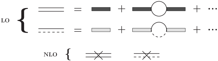
Figure 1: Infinite sum of bubble diagrams that give LO $cn$ and $nn$-dimer propagators. Solid lines are neutrons, dashed lines are cores, light rectangles are bare $cn$-dimer propagators, $i/\Delta_{1}$, and dark rectangles are bare $nn$-dimer propagators, $i/\Delta_{0}$. The NLO dimer propagators receive range corrections represented by a cross.

The infinite sum of diagrams is readily solved via a geometric series yielding the NLO $nn$-dimer propagator

$$D_{nn}(q_{0},q)=\frac{1}{\sqrt{\frac{1}{4}q^{2}-m_{n}q_{0}-i\epsilon}-\gamma_{nn}}\left\{\underbrace{1\vphantom{\frac{Z_{nn}-1}{2\gamma_{nn}}\left(\gamma_{nn}+\sqrt{\frac{2+A}{4A}q^{2}-m_{n}E}\right)}}_{\mathrm{LO}}+\underbrace{\frac{Z_{nn}-1}{2\gamma_{nn}}\left(\gamma_{nn}+\sqrt{\frac{1}{4}q^{2}-m_{n}q_{0}-i\epsilon}\right)}_{\mathrm{NLO}}\right\},$$ (5)

and NLO $cn$-dimer propagator

$$D_{cn}(q_{0},q)=\frac{1}{\sqrt{\frac{A}{(1+A)^{2}}q^{2}-\frac{2A}{1+A}m_{n}q_{0}-i\epsilon}-\gamma_{cn}}$$ (6)

$$\hskip 113.81102pt\times\left\{\underbrace{1\vphantom{\frac{Z_{cn}-1}{2\gamma_{cn}}\left(\gamma_{cn}+\sqrt{\frac{A}{(1+A)^{2}}q^{2}-\frac{2A}{1+A}m_{n}q_{0}}\right)}}_{\mathrm{LO}}+\underbrace{\frac{Z_{cn}-1}{2\gamma_{cn}}\left(\gamma_{cn}+\sqrt{\frac{A}{(1+A)^{2}}q^{2}-\frac{2A}{1+A}m_{n}q_{0}-i\epsilon}\right)}_{\mathrm{NLO}}\right\},$$

where $A=\frac{m_{c}}{m_{n}}$. Parameters of the dimer propagators are fit using the $Z$-parametrization Phillips et al. (2000); Grießhammer (2004), which fits to the pole in the two-body scattering amplitude at LO and to its residue at NLO. The parameter $\gamma_{nn}$ is fit to the $nn$ virtual bound state momentum, which can be related to the $nn$-scattering length, $a_{nn}$, and effective range, $\rho_{nn}$, via Grießhammer (2004)

$$\gamma_{nn}=\frac{1}{a_{nn}}+\frac{\rho_{nn}}{2}\gamma_{nn}^{2}+\cdots$$ (7)

The residue to NLO about the $nn$ virtual bound state pole is given by

$$Z_{nn}=\frac{1}{1-\gamma_{nn}\rho_{nn}}.$$ (8)

Using the values $a_{nn}=-18.7(6)$ fm Gonzalez Trotter et al. (1999) and $\rho_{nn}=2.75(11)$ fm Miller et al. (1990) for the $nn$ scattering length and effective range yields the value $\gamma_{nn}=-9.87$ MeV ($Z_{nn}=1.16$) for the $nn$ virtual bound state momentum (residue).

For the $cn$-dimer, $\gamma_{cn}=\mathrm{sign}(B_{1})\sqrt{2\mu|B_{1}|}$, is fit to the $cn$ system “binding energy”, $B_{1}$. Negative $B_{1}$ values give virtual bound states, and the imaginary part of the binding momentum for such resonant $cn$-states is ignored. The value of the residue, $Z_{cn}$, about the $cn$ pole is given by

$$Z_{cn}=\frac{1}{1-\gamma_{cn}\rho_{cn}}$$ (9)

where $\rho_{cn}$ is the effective range for $cn$ scattering. Unfortunately, experimental determinations of $\rho_{cn}$ are currently unavailable. Therefore, NLO corrections from $Z_{nn}$ and $Z_{cn}$ will be disentangled, and results will be given for arbitrary values of $Z_{cn}$, which can be used to easily determine charge and matter radii once $\rho_{cn}$ is measured. In addition $\rho_{cn}\sim 1/m_{\pi}=1.4$ fm, will be given a value based on naturalness to make NLO predictions, where $m_{\pi}$ is the pion mass.

Finally the parameters in the two-body Lagrangian are given by Grießhammer (2004)

$$\Delta_{0}=\gamma_{nn}-\mu_{\mathrm{PDS}}, w_{0}=(Z_{nn}-1)\frac{m_{n}}{2\gamma_{nn}}, g_{0}^{2}=\frac{4\pi}{m_{n}}$$ (10)

$$\Delta_{1}=\gamma_{cn}-\mu_{\mathrm{PDS}}, w_{1}=(Z_{cn}-1)\frac{\mu}{\gamma_{cn}}, g_{1}^{2}=\frac{2\pi}{\mu}.$$

The scale $\mu_{\mathrm{PDS}}$ comes from using dimensional regularization with the power divergence subtraction technique Kaplan et al. (1998a, b) for all loop integrals.

IV Three-Body System

Calculation of bound state properties of two-neutron halo nuclei requires the three-body wavefunction, which is directly related to the trimer vertex function. The LO trimer vertex function is given by the coupled integral equations in Fig. 2

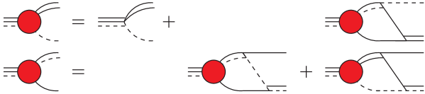
Figure 2: Coupled integral equations for LO trimer vertex function. The trimer field is given by the triple line and the trimer vertex function the the red circle.

, which give the matrix equation

$$\boldsymbol{\mathcal{G}}_{0}(E,p)=\mathbf{B}+\Big{[}\mathbf{R}_{0}(E,p,q)\mathbf{D}(E,q)\Big{]}\otimes\boldsymbol{\mathcal{G}}_{0}(E,q),$$ (11)

where the “$\otimes$” operator is defined by

$$A(q)\otimes B(q)=\frac{1}{2\pi^{2}}\int_{0}^{\Lambda}dqq^{2}A(q)B(q).$$ (12)

$\Lambda$ is a cutoff used to regulate potential divergences. Once properly renormalized all physical quantities should have a well defined limit in the limit $\Lambda\to\infty$. $\mathbf{B}$ the inhomogenous term and $\boldsymbol{\mathcal{G}}_{0}(E,p)$ the LO trimer vertex function are both vectors defined by

$$\mathbf{B}=\left(\begin{array}[]{c}1\\[-5.69054pt] 0\end{array}\right)\quad,\quad\boldsymbol{\mathcal{G}}_{m}(E,p)=\left(\begin{array}[]{c}\mathcal{G}_{m,t\to d_{0}c}(E,p)\\[-5.69054pt] \mathcal{G}_{m,t\to d_{1}n}(E,p)\end{array}\right),$$ (13)

where $\mathcal{G}_{m,t\to d_{0}c}(E,p)$ ($\mathcal{G}_{m,t\to d_{1}n}(E,p)$) is the vertex function for a trimer going to a spectator core and $nn$-dimer (spectator neutron and $cn$-dimer). The subscript “$m$” refers to the order of the trimer vertex function (i.e. $m=0$ is LO, $m=1$ is NLO, etc…). The kernel term $\mathbf{R}_{0}(E,p,q)$ is a matrix defined by

$$\mathbf{R}_{0}(E,p,q)=\left(\begin{array}[]{cc}R_{00}(E,p,q)&R_{01}(E,p,q)\\ R_{10}(E,p,q)&R_{11}(E,p,q)\\ \end{array}\right),$$ (14)

where

$$R_{00}(E,p,q)=0,$$ (15)

$$R_{01}(E,p,q)=\frac{2\sqrt{2}\pi(1\!+\!A)}{A}\frac{1}{pq}Q_{0}\left(\frac{\frac{1+A}{2A}p^{2}+q^{2}-m_{n}E}{pq}\right),$$ (16)

$$R_{10}(E,p,q)=R_{01}(E,q,p),$$ (17)

and

$$R_{11}(E,p,q)=\frac{(1\!+\!A)^{2}\pi}{A}\frac{1}{pq}Q_{0}\left(\frac{\frac{(1+A)}{2}(p^{2}+q^{2})-Am_{n}E}{pq}\right).$$ (18)

$Q_{0}(a)$ is a Legendre function of the second kind defined by

$$Q_{0}(a)=\frac{1}{2}\ln\left(\frac{1+a}{a-1}\right).$$ (19)

Finally $\mathbf{D}(E,q)$ is a matrix of LO dimer propagators given by

$$\mathbf{D}(E,q)=\left(\begin{array}[]{cc}\bar{D}_{nn}^{(0)}(E,q)&0\\ 0&\bar{D}_{cn}^{(0)}(E,q)\\ \end{array}\right),$$ (20)

with

$$\bar{D}_{nn}^{(m)}(E,q)=D_{nn}^{(m)}\left(E-\frac{q^{2}}{2Am_{n}},q\right)\quad,\quad\bar{D}_{cn}^{(m)}(E,q)=\frac{2A}{1+A}D_{cn}^{(m)}\left(E-\frac{q^{2}}{2m_{n}},q\right),$$ (21)

where the superscript “($m$)” refers to only the LO (NLO) part of Eqs. (5) and (6) for $m=0$ ($m=1$).

The NLO correction to the trimer vertex function receives range corrections as shown in the coupled integral equations of Fig. 3

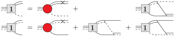
Figure 3: Coupled integral equations for the NLO correction to the trimer vertex function. The box with a “1” inside represents the NLO correction to the trimer vertex function.

This set of coupled integral equations gives the matrix equation

$$\boldsymbol{\mathcal{G}}_{1}(E,p)=\mathbf{R}_{1}(E,p)\boldsymbol{\mathcal{G}}_{0}(E,p)+\Big{[}\mathbf{R}_{0}(E,p,q)\mathbf{D}(E,q)\Big{]}\otimes\boldsymbol{\mathcal{G}}_{1}(E,q),$$ (22)

where the matrix $\mathbf{R}_{1}(E,p)$ is

$$\mathbf{R}_{1}(E,p)=\left(\begin{array}[]{cc}\frac{Z_{nn}-1}{2\gamma_{nn}}\left(\gamma_{nn}+\sqrt{\frac{2+A}{4A}p^{2}-m_{n}E}\right)&0\\[5.69054pt] 0&\frac{Z_{cn}-1}{2\gamma_{cn}}\left(\gamma_{cn}+\sqrt{\frac{A(2+A)}{(1+A)^{2}}p^{2}-\frac{2A}{1+A}m_{n}E}\right)\end{array}\right).$$ (23)

Finally, the trimer wavefunction renormalization up to NLO is given by

$$Z_{t}=\frac{1}{\Sigma_{0}^{\prime}(E)}\left[\underbrace{1\vphantom{\frac{\Sigma_{1}^{\prime}(E)}{\Sigma_{0}^{\prime}(E)}}}_{\mathrm{LO}}-\underbrace{\frac{\Sigma_{1}^{\prime}(E)}{\Sigma_{0}^{\prime}(E)}}_{\mathrm{NLO}}+\cdots\right],$$ (24)

where $\Sigma_{m}(E)$ are the order-by-order corrections to the trimer self energy defined by Vanasse (2015)

$$\Sigma_{m}(E)=\frac{m_{n}}{2}\mathcal{G}_{m,t\to d_{0}c}(E,q)\otimes\bar{D}_{nn}^{(0)}(E,q).$$ (25)

The functions $\Sigma_{0}(E)$ and $\Sigma_{1}(E)$ are given by the diagrams in Fig. 4.

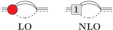
Figure 4: Diagrams representing the LO $\Sigma_{0}(E)$ and NLO $\Sigma_{1}(E)$.

Fitting the energy, $E=B_{cnn}$, to the $cnn$ bound state energy, $B_{cnn}$, yields the values

$$\frac{h_{0}^{2}}{\Omega}=\frac{1}{\Sigma_{0}(E)}\quad,\quad\frac{2h_{1}h_{0}}{\Omega}=-\frac{\Sigma_{1}(E)}{\left(\Sigma_{0}(E)\right)^{2}},$$ (26)

for the parameters in the three-body Lagrangian Vanasse (2015). However, for the purposes of this calculation the values of three-body forces are not relevant, but only the values of $\Sigma_{0}^{\prime}(E)$, and $\Sigma_{1}^{\prime}(E)$ are relevant. Finally, we define the quantity $Z_{t}^{\mathrm{LO}}$ as

$$Z_{t}^{\mathrm{LO}}=\frac{1}{\Sigma_{0}^{\prime}(E)}.$$ (27)

V Charge and Matter Form Factors

The LO charge form factor of two-neutron halo nuclei is given by the sum of diagrams in Fig. 5, where the blue wavy lines represent minimally coupled $A_{0}$ photons that only couple to the charged core.

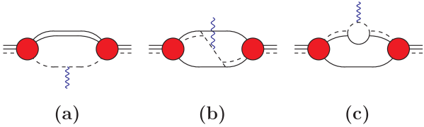
Figure 5: Diagrams for the LO charge form factor of two-neutron halo nuclei. The wavy blue lines represent minimally coupled $A_{0}$ photons.

Meanwhile, the LO neutron form factor of two-neutron halo nuclei is given by the sum of diagrams in Fig. 6, where the green zig-zag is a fictitious current that couples to neutrons with a charge of one. For the neutron form factor their are two different type (c) diagrams, one for an intermediate $cn$-dimer and the other for an intermediate $nn$-dimer. All form factors are calculated in the Breit frame in which the external current only imparts momentum, but no energy. Form factors only depend on the external current exchange momentum squared, $\vec{\mathbf{Q}}^{2}=(\vec{\mathbf{P}}-\vec{\mathbf{K}})^{2}$, where $\vec{\mathbf{K}}$ ($\vec{\mathbf{P}}$) is the trimer momentum before (after) the external current.

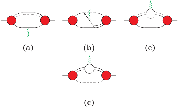
Figure 6: Diagrams for the LO neutron form factor of two-neutron halo nuclei. The green zig-zags represent an external current that only couples to neutrons. Note there are two (c) type diagrams, one with an intermediate $cn$-dimer and the other with an intermediate $nn$-dimer.

The LO diagram (a) contribution for both charge and neutron form factors is given by

$$F_{0}^{(a;X)}(Q^{2})=Z_{t}^{\mathrm{LO}}\left\{\widetilde{\boldsymbol{\mathcal{G}}}_{0}^{T}(p)\otimes\boldsymbol{\mathcal{A}}_{0}^{(X)}(p,k,Q)\otimes\widetilde{\boldsymbol{\mathcal{G}}}_{0}(k)+2\widetilde{\boldsymbol{\mathcal{G}}}_{0}^{T}(p)\otimes\boldsymbol{\mathcal{A}}_{0}^{(X)}(p,Q)+\mathcal{A}_{0}^{(X)}(Q)\right\},$$ (28)

where the superscript $X\!=\!C$ ($X\!=\!n$) for the charge (neutron) form factor. Functions $\boldsymbol{\mathcal{A}}_{m}^{(X)}(p,k,Q)$, $\boldsymbol{\mathcal{A}}_{m}^{(X)}(p,Q)$, and $\mathcal{A}_{m}^{(X)}(Q)$ are a matrix, vector, and scalar respectively and are defined in Appendix A. The vector $\widetilde{\boldsymbol{\mathcal{G}}}_{m}(p)$ is defined as

$$\widetilde{\boldsymbol{\mathcal{G}}}_{m}(p)=\mathbf{D}(E,p)\boldsymbol{\mathcal{G}}_{m}(E,p).$$ (29)

Diagram (b) gives the contribution

$$F_{0}^{(b;X)}(Q^{2})=Z_{t}^{\mathrm{LO}}\widetilde{\boldsymbol{\mathcal{G}}}_{0}^{T}(p)\otimes\boldsymbol{\mathcal{B}}_{0}^{(X)}(p,k,Q)\otimes\widetilde{\boldsymbol{\mathcal{G}}}_{0}(k),$$ (30)

to the charge and neutron form factors, where $\boldsymbol{\mathcal{B}}_{0}^{(X)}(p,k,Q)$ is a matrix defined in Appendix A. The function $\boldsymbol{\mathcal{B}}_{0}^{(X)}(p,k,Q)$ does not receive higher order corrections. Finally, the contribution from (c) type diagrams to charge and neutron form factors is given by

$$F_{0}^{(c;X)}(Q^{2})=Z_{t}^{\mathrm{LO}}\left\{\widetilde{\boldsymbol{\mathcal{G}}}_{0}^{T}(p)\otimes\boldsymbol{\mathcal{C}}_{0}^{(X)}(p,k,Q)\otimes\widetilde{\boldsymbol{\mathcal{G}}}_{0}(k)+\boldsymbol{\mathcal{C}}_{0}^{(X)}(k,Q)\otimes\widetilde{\boldsymbol{\mathcal{G}}}_{0}(k)+\mathcal{C}_{0}^{(X)}(Q)\right\},$$ (31)

where $\boldsymbol{\mathcal{C}}_{m}^{(X)}(p,k,Q)$ is a matrix, $\boldsymbol{\mathcal{C}}_{m}^{(X)}(k,Q)$ a vector, and $\mathcal{C}_{m}^{(X)}(Q)$ a scalar defined in Appendix A. Combining the contributions from (a) through (c) type diagrams yields the LO charge and neutron form factors

$$F_{0}^{(X)}(Q^{2})=F_{0}^{(a;X)}(Q^{2})+F_{0}^{(b;X)}(Q^{2})+F_{0}^{(c;X)}(Q^{2}).$$ (32)

The NLO correction to the two-neutron halo nuclei charge form factor is given by the sum of diagrams in Fig. 7. Diagram (d) comes from gauging the $cn$-dimer kinetic term in Eq. (1).

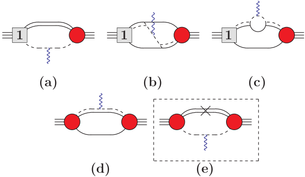
Figure 7: Diagrams for NLO correction to the charge form factor for two-neutron halo nuclei. The boxed diagram (e) is subtracted to avoid double counting from diagram (a) and its time reversed version, and diagram (d) comes from gauging the $cn$-dimer kinetic term. Diagrams related by time reversal symmetry are not shown.

The NLO correction to the two-neutron halo nuclei neutron form factor is given by the sum of diagrams in Fig. 8, where the coupling for the (d) type diagrams comes from gauging the $nn$- and $cn$-dimer kinetic terms in Eq. (1). In Figs. 7 and 8 diagrams related by time reversal symmetry are not shown, and diagram (e) is subtracted to avoid double counting from diagram (a) and its time reversed version.

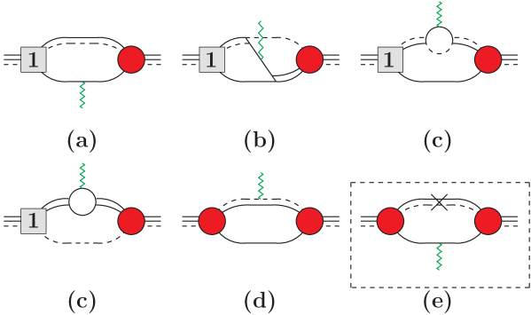
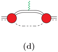
Figure 8: Diagrams for the NLO correction to the neutron form factor for two-neutron halo nuclei. The boxed diagram (e) is subtracted to avoid double counting. Note, there are two type (c) and type (d) diagrams. Diagrams related by time reversal symmetry are not shown

The NLO correction to the charge and neutron form factor from diagram (a) minus diagram (e) is given by

$$F_{1}^{(a;X)}(Q^{2})=Z_{t}^{\mathrm{LO}}\left\{\widetilde{\boldsymbol{\mathcal{G}}}_{0}^{T}(p)\otimes\boldsymbol{\mathcal{A}}_{1}^{(X)}(p,k,Q)\otimes\widetilde{\boldsymbol{\mathcal{G}}}_{0}(k)+2\widetilde{\boldsymbol{\mathcal{G}}}_{1}^{T}(p)\otimes\boldsymbol{\mathcal{A}}_{0}^{(X)}(p,k,Q)\otimes\widetilde{\boldsymbol{\mathcal{G}}}_{0}(k)\right.$$ (33)

$$\left.\hskip 142.26378pt+2\widetilde{\boldsymbol{\mathcal{G}}}_{0}^{T}(p)\otimes\boldsymbol{\mathcal{A}}_{1}^{(X)}(p,Q)+2\widetilde{\boldsymbol{\mathcal{G}}}_{1}^{T}(p)\otimes\boldsymbol{\mathcal{A}}_{0}^{(X)}(p,Q)+\mathcal{A}_{1}^{(X)}(Q)\right\}.$$

NLO corrections to the charge and neutron form factors from diagram (b) yield

$$F_{1}^{(b;X)}(Q^{2})=Z_{t}^{\mathrm{LO}}\left\{2\widetilde{\boldsymbol{\mathcal{G}}}_{1}^{T}(p)\otimes\boldsymbol{\mathcal{B}}_{0}^{(X)}(p,k,Q)\otimes\widetilde{\boldsymbol{\mathcal{G}}}_{0}(k)\right\},$$ (34)

and from diagrams (c)

$$F_{1}^{(c;X)}(Q^{2})=Z_{t}^{\mathrm{LO}}\left\{\widetilde{\boldsymbol{\mathcal{G}}}_{0}^{T}(p)\otimes\boldsymbol{\mathcal{C}}_{1}^{(X)}(p,k,Q)\otimes\widetilde{\boldsymbol{\mathcal{G}}}_{0}(k)+\widetilde{\boldsymbol{\mathcal{G}}}_{1}^{T}(p)\otimes\boldsymbol{\mathcal{C}}_{0}^{(X)}(p,k,Q)\otimes\widetilde{\boldsymbol{\mathcal{G}}}_{0}(k)\right.$$ (35)

$$\hskip 142.26378pt+\widetilde{\boldsymbol{\mathcal{G}}}_{0}^{T}(p)\otimes\boldsymbol{\mathcal{C}}_{0}^{(X)}(p,k,Q)\otimes\widetilde{\boldsymbol{\mathcal{G}}}_{1}(k)+\boldsymbol{\mathcal{C}}_{1}^{(X)}(k,Q)\otimes\widetilde{\boldsymbol{\mathcal{G}}}_{0}(k)$$

$$\left.\hskip 256.0748pt+\boldsymbol{\mathcal{C}}_{0}^{(X)}(k,Q)\otimes\widetilde{\boldsymbol{\mathcal{G}}}_{1}(k)+\mathcal{C}_{1}^{(X)}(Q)\right\}.$$

At NLO there are new contributions from (d) type diagrams to the charge and neutron form factors which give

$$F_{1}^{(d;X)}(Q^{2})=Z_{t}^{\mathrm{LO}}\left\{\widetilde{\boldsymbol{\mathcal{G}}}_{0}^{T}(p)\otimes\boldsymbol{\mathfrak{D}}_{1}^{(X)}(p,k,Q)\otimes\widetilde{\boldsymbol{\mathcal{G}}}_{0}(k)+\boldsymbol{\mathfrak{D}}_{1}^{(X)}(k,Q)\otimes\widetilde{\boldsymbol{\mathcal{G}}}_{0}(k)+\mathfrak{D}_{1}^{(X)}(Q)\right\},$$ (36)

where $\boldsymbol{\mathfrak{D}}_{1}^{(X)}(p,k,Q)$ is a matrix, $\boldsymbol{\mathfrak{D}}_{1}^{(X)}(k,Q)$ a vector, and $\mathfrak{D}_{1}^{(X)}(Q)$ a scalar defined in Appendix A. Combining the contribution from diagrams (a) through (d) and multiplying the LO form factor by the NLO trimer wavefunction renormalization gives the NLO correction to the charge and neutron form factors

$$F_{1}^{(X)}(Q^{2})=\left(F_{1}^{(a;X)}(Q^{2})+F_{1}^{(b;X)}(Q^{2})+F_{1}^{(c;X)}(Q^{2})+F_{1}^{(d;X)}(Q^{2})\right)-\frac{\Sigma_{1}^{\prime}(E)}{\Sigma_{0}^{\prime}(E)}F_{0}^{(X)}(Q^{2}).$$ (37)

VI Observables

Expanding the LO two-neutron halo nuclei charge form factor as a function of $Q^{2}$ yields

$$F_{0}^{(C)}(Q^{2})=1-\frac{1}{6}\left<r_{C}^{2}\right>_{0}Q^{2}+\cdots$$ (38)

where $\left<r_{C}^{2}\right>_{0}$ is the LO point charge radius squared of the $cnn$ system. The LO neutron form factor expanded in powers of $Q^{2}$ yields

$$F_{0}^{(n)}(Q^{2})=2\left(1-\frac{1}{6}\left<r_{n}^{2}\right>_{0}Q^{2}+\cdots\right)$$ (39)

where $\left<r_{n}^{2}\right>_{0}$ is the LO neutron radius of the $cnn$ system. Expanding in powers of $Q^{2}$ the NLO correction to the charge form factor is given by

$$F_{1}^{(C)}(Q^{2})=-\frac{1}{6}\left<r_{C}^{2}\right>_{1}Q^{2}+\cdots,$$ (40)

and the NLO correction to the neutron form factor by

$$F_{1}^{(n)}(Q^{2})=2\left(-\frac{1}{6}\left<r_{n}^{2}\right>_{1}Q^{2}+\cdots.\right),$$ (41)

where $\left<r_{n}^{2}\right>_{1}$ ($\left<r_{C}^{2}\right>_{1}$) is the NLO correction to the neutron (point charge) radius of the $cnn$ system. Due to gauge invariance the NLO correction to the form factors are zero at $Q^{2}=0$ and this is observed numerically to at least seven digits. Likewise it is observed that $F_{0}^{(C)}(0)=1$ and $F_{0}^{(n)}(0)=2$ to at least seven digits.

The point charge radius squared of the $cnn$ system is related to its physical charge radius squared, $\left<r_{C}^{2}\right>^{cnn}$, by

$$\left<r_{C}^{2}\right>^{cnn}=\left<r_{C}^{2}\right>+\left<r_{C}^{2}\right>^{c}+\frac{2}{Z}\left<r_{C}^{2}\right>^{n},$$ (42)

where $\left<r_{C}^{2}\right>^{c}$ is the charge radius squared of the core, $Z$ the number of protons in the core, and $\left<r_{C}^{2}\right>^{n}=-0.115(4)$ fm² Olive et al. (2014) is the charge radius squared of the neutron. In isotope shift experiments using laser spectroscopy the value of $\left<r_{C}^{2}\right>$ is directly accessible if the relatively small contribution from the neutron charge radius squared is ignored Sanchez et al. (2006). The point matter radius of the $cnn$ system is obtained from the charge and neutron radius via

$$\sqrt{\left<r_{M}^{2}\right>}=\sqrt{\frac{1}{2\!+\!A}\left((A\left<r_{C}^{2}\right>+2\left<r_{n}^{2}\right>\right)},$$ (43)

and the physical matter radius squared, $\left<r_{M}^{2}\right>^{cnn}$, of the $cnn$ system is related to the point matter radius squared by

$$\left<r_{M}^{2}\right>^{cnn}=\left<r_{M}^{2}\right>+\frac{A}{2\!+\!A}\left<r_{M}^{2}\right>^{c}+\frac{2}{2\!+\!A}\left<r_{M}^{2}\right>^{n},$$ (44)

where $\left<r_{M}^{2}\right>^{c}$ is the matter radius squared of the core and $\left<r_{M}^{2}\right>^{n}$ is the matter radius squared of the neutron. The small contribution from the neutron is ignored.

Two-neutron halo nuclei can be understood geometrically as in Fig. 9.

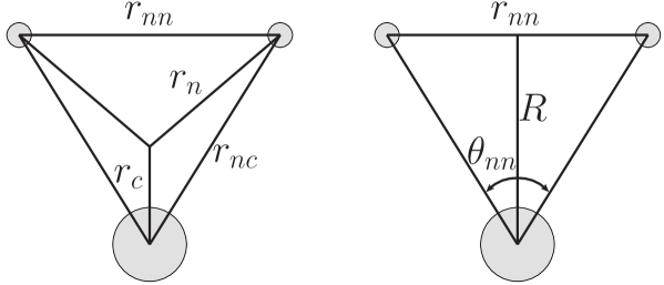
Figure 9: Geometric representation of two-neutron halo nucleus. The value $r_{c}$ is the charge radius and $r_{n}$ the neutron radius, which both extend from from the c.m. of the two-neutron halo nucleus to the core (large circle) and neutron (small circle) respectively.

The large circle represents the core and the smaller circles the valence neutrons. $r_{c}$ is the point charge radius that extends from the center of mass (c.m.) of the $cnn$ system to the core, and $r_{n}$ is the neutron radius. Writing all other geometrical quantities in Fig. 9 in terms of $r_{c}$, $r_{n}$, and $A$ gives

$$R=\frac{2+A}{2}r_{c}$$ (45)

for the average distance between the core and the $nn$ center of mass,

$$r_{nn}=2\sqrt{r_{n}^{2}-\left(\frac{A}{2}r_{c}\right)^{2}}$$ (46)

for the average inter-neutron separation,

$$r_{nc}=\sqrt{r_{n}^{2}+\frac{2+A}{2}r_{c}^{2}}$$ (47)

for the average core neutron separation, and

$$\theta_{nn}=2\arctan\left(\frac{r_{nn}}{(2+A)r_{c}}\right)$$ (48)

for the neutron opening angle. These geometrical quantities prove useful as they are more accessible in certain experiments and also have widespread adoption in the literature.

VII Results

The LO calculation of the neutron and charge form factors only requires four two-body inputs and one piece of three-body data. In the $nn$ channel there is the $nn$ virtual bound state energy, $\gamma_{nn}=-9.87$ MeV, and the neutron mass. While in the $cn$ channel there is the core mass and $cn$ “binding energy”, $B_{cn}$, given in Table 1 for halo nuclei considered in this work. For unbound $cn$ systems $|B_{cn}|$ is given by the real part of the lowest lying resonance for $cn$ scattering and $B_{cn}$ is negative. Using the $cnn$ system binding energy given in Table 1 the three-body force is fixed at LO and NLO. In addition the quantum numbers of the core, $cn$ system, and bound $cnn$ system are shown in Table 1. The Lithium system does not have a spin zero core as assumed in our formalism. However, since the core is much heavier than the neutrons the static limit in which the core spin is unchanged can be used to approximate the core as spin zero. Other two-neutron halo nuclei such as ⁶He and ¹⁷B are not considered here as they are dominated by two-body $P$-wave interactions and will be dealt with in future work. At NLO only the two-body $nn$ effective range $\rho_{nn}$ and $cn$ effective range $\rho_{cn}$ are needed.

Nucleus	$m_{C}$ [MeV]	$B_{cn}$ [MeV]	$B_{cnn}$ [MeV]	$J_{c}^{\pi}:J_{cn}^{\pi}:J_{cnn}^{\pi}$
9-11Li	8408	-0.026(13)	0.3693(6)	$3/2^{-}$:$(2^{-},1^{-})$:$3/2^{-}$
12-14Be	11203	-0.510	1.27(13)	$0^{+}$:($1/2^{-}$):$0^{+}$
20-22C	18667	-0.01(47) Wang et al. (2012)	0.11(6) Wang et al. (2012)	$0^{+}$:$(1/2^{+})$:$0^{+}$

Table 1: The mass $m_{c}$ and quantum numbers, $J^{\pi}_{c}$, of the ⁹Li, ¹²Be, and ²⁰C core are given. Binding energies, $B_{cn}$ and quantum numbers, $J^{\pi}_{cn}$, of the ¹⁰Li, ¹³Be, and ²¹C resonances are given and the bound state energies, $B_{cnn}$ and quantum numbers, $J^{\pi}_{cnn}$, of the halo nuclei ¹¹Li, ¹⁴Be, and ²²C. The quantum number $J$ is the total angular momentum and $\pi$ the parity. All numbers without a reference come from Ref. NuD .

There are three sources of error in the caluclation of the form factors, (i) numerical error, (ii) error from two- and three-body parameters, and (iii) error from the halo-EFT expansion. Numerical error is negligible compared to the other sources of error and will henceforth be disregarded. The predominant source of error for ¹¹Li and ¹⁴Be comes from the halo-EFT expansion, which is estimated in Table 2 for each halo nucleus, where ratios of $M_{hi}$ to $M_{low}$ parameters are taken. The scales for $M_{hi}$ are the core’s first excited state energy, $E_{C}^{*}$, and the one neutron separation energy, $B_{c-n}$, for the core, both shown in Table 2. These scales signal the breakdown of halo-EFT since the core can no longer be a fundamental degree of freedom at these energies. The scales for $M_{low}$ are given by $B_{cn}$ and $B_{cnn}$. Taking the most conservative error estimate we find the error of the EFT expansion is 37% for ¹¹Li, 78% for ¹⁴Be, and 26% for ²²C. However, the error for ²²C is dominated by the uncertainty in $B_{cn}$ and $B_{cnn}$. Since within the error of $B_{cn}$ it can equal $B_{cnn}$ the charge and matter radius of ²²C diverge, and it can only be bounded from below.

Nucleus	$E_{C}^{*}$ [MeV]	$B_{c-n}$ [MeV]	$\sqrt{|B_{cn}/E_{C}^{*}|}$	$\sqrt{B_{cnn}/E_{C}^{*}}$	$\sqrt{|B_{cn}/B_{c-n}|}$	$\sqrt{|B_{cnn}/B_{c-n}|}$
9-11Li	2.69	4.06	0.098	0.370	0.078	0.301
12-14Be	2.10	3.17	0.493	0.78	0.40	0.63
20-22C	1.59 Stanoiu et al. (2008)	2.9(3)	0.09	0.26	0.07	0.19

Table 2: The first excited state energy $E_{c}^{*}$ and the one neutron separation energy $B_{c-n}$ of the ⁹Li, ¹²Be, and ²⁰C cores are given. Using these values the ratios $\sqrt{|B_{cn}/E_{C}^{*}|}$, $\sqrt{|B_{cnn}/E_{c}^{*}|}$, $\sqrt{|B_{cn}/B_{c-n}|}$, and $\sqrt{|B_{cn}/B_{c-n}|}$ are calculated to estimate the error of the halo-EFT expansion. All numbers for $E_{C}^{*}$ and $B_{c-n}$ without a reference come from Ref. NuD .

The LO and NLO predictions for the point charge radius, point matter radius, and existing experimental determinations are shown in Table 3 for each halo nucleus.

Nucleus	$\left<r_{C}^{2}\right>_{0}$ fm2	$\left<r_{M}^{2}\right>_{0}$ fm2	$\left<r_{C}^{2}\right>_{0+1}$ fm2	$\left<r_{M}^{2}\right>_{0+1}$ fm2	$\left<r_{C}^{2}\right>$-Exp. fm2	$\left<r_{M}^{2}\right>$-Exp. fm2
11Li	$0.744(275)$	$5.76\pm 2.13$	$0.774(106)$	$6.05\pm 0.83$	1.171(120) Sanchez et al. (2006) 1.104(85) Puchalski et al. (2006) 0.82(11) Esbensen et al. (2007); Nakamura et al. (2006)	$5.34\pm 0.15$ Ozawa et al. (2001a)
14Be	$0.126(98)$	$1.23\pm 0.96$	$0.134(81)$	$1.34\pm 0.81$	—	$4.24\pm 2.42$ Ozawa et al. (2001a) $2.90\pm 2.25$ Ozawa et al. (2001a)
22C	$0.520^{+\infty}_{-0.274}$	$9.00^{+\infty}_{-5.01}$	$0.530^{+\infty}_{-0.283}$	$9.22^{+\infty}_{-5.16}$	—	$21.1\pm 9.7$ Ozawa et al. (2001b); Tanaka et al. (2010) $3.77\pm 0.61$ Ozawa et al. (2001b); Togano et al. (2016)

Table 3: LO and NLO halo-EFT predicitions for charge and mater radii of two-neutron halo nuclei. Included are existing experimental results. The NLO results use the naturalness estimate $\rho_{cn}\sim 1/m_{\pi}\sim 1.4$ fm for the NLO prediction, where $\rho_{cn}$ is the effective range for $cn$ scattering.

All results are calculated at a cutoff of $\Lambda=20000$ MeV, which is sufficient to ensure convergence with respect to $\Lambda$. The radii are extracted from the form factors by performing a linear fit with respect to $Q^{2}$ over the range $Q^{2}=0-0.5$ MeV². At NLO the $cn$ effective range, $\rho_{cn}$, is estimated using naturalness assumptions giving the value $\rho_{cn}\sim 1/m_{\pi}=1.4$ fm. Atomic spectroscopy gives the experimental value of $1.171(120)$ fm² for the ¹¹Li point charge radius squared Sanchez et al. (2006). This value was later revised in Ref. Puchalski et al. (2006) by adding finite mass corrections giving a value of 1.104(85) fm². Using the cluster sum rule Bertsch and Esbensen (1991) the experimental electric dipole response of ¹¹Li Nakamura et al. (2006) can be related to its point charge radius squared yielding a value of $0.82(11)$ fm² Esbensen et al. (2007). Our LO prediction for the ¹¹Li point charge radius of $0.744(275)$ fm² squared agrees with the smaller experimental value within errors, and NLO corrections, assuming a natural value for $\rho_{cn}$, give $0.774(106)$ fm² again agreeing with the smaller experimental number within errors. The difference between these experimental values is often attributed to polarization effects of the core Esbensen et al. (2007), which occur at orders beyond NLO in halo-EFT. In addition realistic values of $\rho_{cn}$ may alleviate some of the disagreement with atomic spectroscopy measurements. Range corrections are found to be an important contribution for the triton charge radius in $\mathrm{EFT}(\not{\pi})$ Vanasse (2015).

The point charge radius squared of ¹⁴Be is $0.126(98)$ fm² at LO and $0.134(81)$ fm² at NLO, while for ²²C we find $0.520^{+\infty}_{-0.274}$ fm² at LO and $0.530^{+\infty}_{-0.283}$ fm² at NLO. The range for ²²C comes from varying $B_{cn}$ and $B_{cnn}$ within their experimental errors. Unfortunately, no experimental determination of the charge radius currently exists for ¹⁴Be or ²²C. Our results for the point charge radius of ¹¹Li, ¹⁴Be, and ²²C disagree with those of Hagen et al. Hagen et al. (2013a). However, if we change the coefficient of a single $Q^{2}$ term in diagram (a) of Fig. 5 then we reproduce the charge radii of Hagen et al. and moreover agree with their expressions for the diagrams in Fig. 5. For further details of this difference see Appendix A.

The point matter radius squared of ¹¹Li is $5.76\pm 2.13$ fm² at LO and $6.05\pm 0.83$ fm² at NLO. This agrees well with the experimental number for the ¹¹Li point matter radius of $5.34\pm 0.15$ fm², which is given by the matter radius of $2.32\pm 0.02$ fm Ozawa et al. (2001a) for ⁹Li, the matter radius of $3.12\pm 0.02$ fm Ozawa et al. (2001a) for ¹¹Li, and the use of Eq. (44). In Eq. (44) the unknown matter radius of the neutron is ignored since it is suppressed by a factor of $2/(2\!+\!A)$. For ¹⁴Be we find a LO point matter radius squared of $1.23\pm 0.96$ fm² and NLO value of $1.34\pm 0.81$ fm², which agrees with the experimental results of $4.24\pm 2.42$ fm² $2.90\pm 2.25$ fm² within the large theoretical and experimental uncertainty. ²²C has a LO point matter radius squared of $9.00^{+\infty}_{-5.01}$ fm² and a NLO matter radius squared of $9.22^{+\infty}_{-5.16}$ fm². The ranges for ²²C, due to varying $B_{cn}$ and $B_{cnn}$ within their experimental errors, overlap with the experimental results of $21.1\pm 9.7$ fm² and $3.77\pm 0.61$ fm². In order to find the experimental point matter radius of ¹⁴Be and ²²C we used Eq. (44), the value $2.59\pm 0.06$ fm Ozawa et al. (2001a) for the ¹²Be matter radius, $3.16\pm 0.38$ fm Ozawa et al. (2001a) and $2.94\pm 0.38$ fm Ozawa et al. (2001a) for the ¹⁴Be matter radius, $2.98\pm 0.05$ fm Ozawa et al. (2001a) for the ²⁰C Ozawa et al. (2001b) matter radius, and $5.4\pm 0.9$ fm Tanaka et al. (2010) and $3.44\pm 0.08$ fm Togano et al. (2016) for the ²²C matter radius. The smaller values for the ¹⁴Be and ²²C matter radii give the smaller experimental values for their respective point matter radii in Table 3.

In addition to the point matter and point charge radii the LO values for the average inter-neutron distance, $r_{nn}$, and neutron opening angle, $\theta_{nn}$, shown in Fig. 9, are given in Table 4. Experimental results of $r_{nn}$ for ¹¹Li and ¹⁴Be from Marqués et al. Marqués et al. (2000, 2001) using two-neutron interferometry agree within errors with our predictions. The neutron opening angles of Bertulani et al. Bertulani and Hussein (2007) are determined using $r_{nn}$ from Marqués et al. Marqués et al. (2000, 2001), atomic spectroscopy data on ¹¹Li for $R$ Sanchez et al. (2006), which gives an angle of $58^{\circ+10}_{-14}$, and dipole response data for ¹¹Li with the cluster sum rule for $R$, which gives an angle of $66^{\circ+22}_{-18}$ Nakamura et al. (2006). For ¹⁴Be Bertulani et al. Bertulani and Hussein (2007) used a model calculation for $R$. The neutron opening angles of Hagino et al. Hagino and Sagawa (2007) use the dipole response data for ¹¹Li with a model to extract $R$, the matter radius of ¹¹Li Ozawa et al. (2001a) to get the neutron opening angle $56.2^{\circ+17.8}_{21.3}$, and the data of Marqués et al. Marqués et al. (2000, 2001) to get $r_{n}$, which gives a value of $65.2^{\circ+11.4}_{-13.0}$. These values agree within errors with our calculated results. However, the error bars are quite large. Also shown in Table 4 are LO halo-EFT predictions from Canham and Hammer Canham and Hammer (2008) for ¹¹Li and ¹⁴Be. For ¹¹Li they find the neutron opening angles $77^{\circ+8}_{-9}$ and $68^{\circ+31}_{-25}$ using different values of $B_{cn}$ and for ¹⁴Be find $72^{\circ+16}_{-13}$. Their values for $\theta_{nn}$ and $r_{nn}$ differ from ours in part due to different choices for the values of $B_{cn}$ and $B_{cnn}$, however, within errors they agree with our results. These calculations were extended to NLO in Ref. Canham and Hammer (2010) by resumming range corrections to all orders and using naturalness assumptions for $\rho_{cn}$. This differs from this work in which range corrections are added perturbatively. NLO values for $\theta_{nn}$ and $r_{nn}$ are not shown because $\theta_{nn}$ barely changes and $r_{nn}$ only slightly.

Nucleus	$r_{nn}$ fm	$\theta_{nn}$ deg.	$r_{nn}$ fm	$\theta_{nn}$ deg.
11Li	7.30${}^{+1.24}_{-1.51}$	75.4${}^{+43.1}_{-36.3}$	$6.6\pm 1.5$ Marqués et al. (2000, 2001) $8.7\pm 0.7$ Canham and Hammer (2008) $6.8\pm 1.8$ Canham and Hammer (2008)	58${}^{+10}_{-14}$, 66${}^{+22}_{-18}$ Bertulani and Hussein (2007) 56.2${}^{+17.8}_{-21.3}$, 65.2${}^{+11.4}_{-13.0}$ Hagino and Sagawa (2007) $77^{+8}_{-9}$, $68^{+31}_{-25}$ Canham and Hammer (2008)
14Be	3.66${}^{+1.22}_{-1.94}$	73.1${}^{+88.0}_{-62.6}$	$5.4\pm 1.0$ Marqués et al. (2000, 2001) $4.1\pm 0.5$ Canham and Hammer (2008)	64${}^{+9}_{-10}$ Bertulani and Hussein (2007) $72^{+16}_{-13}$ Canham and Hammer (2008)
22C	13.0${}^{+\infty}_{-4.72}$	78.8${}^{+101.2}_{-27.3}$	—	—

Table 4: Values of $r_{n}$ and $\theta_{nn}$ for halo nuclei. The error for $r_{nn}$ and $\theta_{nn}$ on ²²C is due to varying the value for $B_{cn}$ and $B_{cnn}$ within their errors.

Table 5 gives the NLO corrections to the charge and matter point radii from the $nn$ and $cn$ effective range corrections separately. The $nn$ NLO range corrections use the physical values for the $nn$ effective range correction, whereas for the $cn$ effective range

$$\frac{Z_{cn}-1}{2\gamma_{cn}}=1\,\mathrm{MeV}^{-1}.$$ (49)

If future experiments determine the $cn$ effective range $\rho_{cn}$ then the value $\frac{Z_{cn}-1}{2\gamma_{cn}}$ can be calculated and multiply the results in Table 5 to get the physical $cn$ NLO range corrections.

Nucleus	$nn$: $\left<r_{C}^{2}\right>_{1}$ fm2	$nn$: $\left<r_{M}^{2}\right>_{1}$ fm2	$cn$: $\left<r_{C}^{2}\right>_{1}$ fm2	$cn$: $\left<r_{M}^{2}\right>_{1}$ fm2
11Li	$3.71\times 10^{-3}$	0.117	7.66	49.2
14Be	$2.05\times 10^{-3}$	$5.94\times 10^{-2}$	1.99	15.1
22C	-(${4.18}^{+\infty}_{-0.587}\times 10^{-4}$)	$6.75^{+\infty}_{-1.02}\times 10^{-2}$	$3.02^{+\infty}_{-2.38}$	$43.8^{+\infty}_{-40.5}$

Table 5: NLO halo-EFT corrections for charge and mater radii of two-neutron halo nuclei. The $nn$: results come from setting $nn$ effective range corrections to their physical values and setting $cn$ effective range corrections to zero, while the $cn$: results come from setting $nn$ effective range corrections to zero and setting the quantity $(Z_{cn}-1)/(2\gamma_{cn})=1~{}\mathrm{MeV}^{-1}$.

Finally, in the unitary and equal mass limit their exists an analytical result Braaten and Hammer (2006) for the point charge and point matter radius squared which states

$$mE\left<r^{2}\right>=\frac{1+s_{0}^{2}}{9}=0.224...,$$ (50)

where $m$ is the mass of the particles, $E$ the three-body binding energy, $\left<r^{2}\right>$ the point charge or point matter radius squared, and $s_{0}\approx 1.00624$ Danilov and Lebedev (1963) is a universal number from the asymptotic solution of the three-boson problem with short range interactions. Taking the equal mass and unitary limit in our code we find the number 0.224 for the combination of parameters in Eq. (50). Note, that any technique that claims to be able to calculate the zero-range limit exactly must obtain this result within numerical accuracy. This number should serve as an essential benchmark for any technique claiming to calculate three-body systems in the zero range approximation.

VIII Conclusion

Using halo-EFT to NLO we have calculated the charge and neutron form factors for the two-neutron halo nuclei ¹¹Li, ¹⁴Be, and ²²C. From the form factors we extracted the point charge and point matter radii to NLO as well as the inter-neutron separation and neutron opening angle to LO. NLO results were obtained using a naturalness assumption for the $cn$ effective range, $\rho_{cn}\sim 1/m_{\pi}=1.4$ fm. At LO and NLO agreement was found between the predicted matter radii and experimental extractions. However, this is partly due to the large error bars in both experiment and theory. Further work will be needed in both theory and experiment to further reduce these error bars. The charge radius of ¹¹Li was found to agree with the experimental extraction from the electric dipole response function of ¹¹Li, but found to slightly under-predict the charge radius from laser spectroscopy. Charge radii for ¹⁴Be and ²²C were also given for which there are no current experimental determinations. Future experiments measuring the charge form factors of halo nuclei are planned for the electron-ion scattering experiment (ELISe) at the Internationl Facility for Antiproton and Ion Research (FAIR) Antonov et al. (2011).

The inter-neutron separation and neutron opening angle were also calculated and compared with experimental extractions. Again agreement was found with “experimental” values, but this is in part due to large error bars. Only LO values are shown for these numbers as the neutron opening angle barely changes at NLO and the inter-neutron separation only slightly. Finally, the NLO corrections to the point charge and point matter radii from the $nn$ effective range $\rho_{nn}$ and the $cn$ effective range $\rho_{cn}$ were calculated separately, such that the point charge and point matter radii can be easily calculated to NLO once $\rho_{cn}$ is measured.

The point charge and point matter radii were also calculated in the unitary equal mass limit and shown to agree with the analytical prediction of Ref. Braaten and Hammer (2006). However, our point charge radii disagree with those of Hagen et al. Hagen et al. (2013a). Comparing our functions for the LO charge form factor with those of Hagen et al. we find a minor discrepancy given in detail in Appendix A. Using the incorrect function from Hagen et al. we reproduce the point charge radii given in their paper, but fail to reproduce the correct value in the unitary and equal mass limit.

In order to have more realistic predictions at NLO the parameter $\rho_{cn}$ must be known. One possible way to measure $\rho_{cn}$ for $n+^{9}$Li is through the breakup process $d(^{9}\mathrm{Li})\to np(^{9}\mathrm{Li})$. Certain kinematical regimes of the three-body breakup spectrum should be especially sensitive to the $n^{9}$Li interaction. A halo-EFT calculation of this process is complicated by the binding energy of the deuteron, 2.22 MeV, being only slightly smaller than the first excited state energy of ⁹Li, 2.69 MeV. The ratio of these two quantities makes for a poor expansion and would likely require that the first excited state of ⁹Li be added as a new degree of freedom. Similar experiments could also be carried out for ¹²Be and ²⁰C. $\rho_{cn}$ could also be determined by ab initio approaches and then combined with halo-EFT Zhang et al. (2014a); Hagen et al. (2013b); Zhang et al. (2014b).

In this work the contribution of two-body $P$-wave interactions was not considered. Such interactions can be added perturbatively as in Ref. Margaryan et al. (2016) for the three-nucleon system. However, for the two-neutron halos ⁶He and ¹⁷B resonant two-body $P$-wave interactions must be treated non-perturabitively Ji et al. (2014). This work also approximated all cores as spin zero, but future work should consider arbitrary spin cores. Further reduction of the theoretical error in halo-EFT will require a NNLO calculation. However, at NNLO a new energy dependent three-body force, $h_{2}$, occurs that will require a new piece of three-body data. The value for $h_{2}$ could be potentially fit to three-body data from ab inito approaches or the asymptotic normalization of the halo nucleus wavefunction. A future NNLO calculation will need to carefully consider appropriate renormalization conditions for $h_{2}$.

Appendix A

The matrix function $\boldsymbol{\mathcal{A}}_{m}^{(C)}(p,k,Q)$ for the diagram (a) contribution in Figs. 5 and 7 to the charge form factor is given by

$$\left[\boldsymbol{\mathcal{A}}_{m}^{(C)}(p,k,Q)\right]_{ij}=\frac{m_{n}^{2}A}{8\pi^{2}}\int_{0}^{\Lambda}\!\!dqq^{2}\int_{0}^{1}\!\!dx\frac{1}{qQx}\left\{R_{i0}\left(E+\frac{qQx}{m_{n}A},k,d(q,Q,x)\right)\right.$$ (51)

$$\hskip 56.9055pt\times R_{0j}\left(E,d(q,Q,-x),p\right)\bar{D}_{nn}^{(m)}\left(E+\frac{qQx}{2m_{n}A}-\frac{Q^{2}}{4m_{n}A(2+A)},q\right)$$

$$\hskip 28.45274pt\left.-R_{i0}\left(E,k,d(q,Q,x)\right)R_{0j}\left(E-\frac{qQx}{m_{n}A},d(q,Q,-x),p\right)\right.$$

$$\left.\hskip 170.71652pt\times\bar{D}_{nn}^{(m)}\left(E-\frac{qQx}{2m_{n}A}-\frac{Q^{2}}{4m_{n}A(2+A)},q\right)\right\}\delta_{j1}\delta_{i1},$$

where $i,j=0,1$ label the matrix components, and $m=0$ ($m=1$) gives the LO contribution (NLO correction). $\boldsymbol{\mathcal{A}}_{m}^{(C)}(p,Q)$ the vector function is given by

$$\left[\boldsymbol{\mathcal{A}}_{m}^{(C)}(p,Q)\right]_{j}=\frac{m_{n}^{2}A}{8\pi^{2}}\int_{0}^{\Lambda}\!\!dqq^{2}\int_{0}^{1}\!\!dx\frac{1}{qQx}\left\{R_{0j}\left(\frac{qQx}{m_{n}A}+E,d(q,Q,x),p\right)\right.$$ (52)

$$\hskip 56.9055pt\times\bar{D}_{nn}^{(m)}\left(E+\frac{qQx}{2m_{n}A}-\frac{Q^{2}}{4m_{n}A(2+A)},q\right)$$

$$\hskip 28.45274pt\left.-R_{0j}\left(E,d(q,Q,x),p\right)\bar{D}_{nn}^{(m)}\left(E-\frac{qQx}{2m_{n}A}-\frac{Q^{2}}{4m_{n}A(2+A)},q\right)\right\}\delta_{1j},$$

and the scalar function $\mathcal{A}_{m}^{(C)}(Q)$ by

$$\mathcal{A}_{m}^{(C)}(Q)=\frac{m_{n}^{2}A}{8\pi^{2}}\int_{0}^{\Lambda}\!\!dqq^{2}\int_{0}^{1}\!\!dx\frac{1}{qQx}\left\{\bar{D}_{nn}^{(m)}\left(E+\frac{qQx}{2m_{n}A}-\frac{Q^{2}}{4m_{n}A(2+A)},q\right)\right.$$ (53)

$$\left.-\bar{D}_{nn}^{(m)}\left(E-\frac{qQx}{2m_{n}A}-\frac{Q^{2}}{4m_{n}A(2+A)},q\right)\right\},$$

where

$$d(q,Q,x)=\sqrt{q^{2}+\frac{2qQx}{2+A}+\frac{Q^{2}}{(2+A)^{2}}}.$$ (54)

For details of how to calculate the functions in this appendix consult Refs. Hagen et al. (2013a); Vanasse (2015). The LO functions $\boldsymbol{\mathcal{A}}_{0}^{(C)}(p,k,Q)$, $\boldsymbol{\mathcal{A}}_{0}^{(C)}(p,Q)$, and $\mathcal{A}_{0}^{(C)}(Q)$ almost agree with the related functions of Hagen et al. Hagen et al. (2013a), however, where we find the value $Q^{2}/(4m_{n}A(2+A))$ in the $nn$-dimer propagator they find $Q^{2}/(8m_{n}A)$. Using their value for the $Q^{2}$ term we are able to reproduce the point charge radii given in their paper. However, using their $Q^{2}$ value gives the wrong point charge radius in the equal mass and unitary limit, whereas our $Q^{2}$ value gives the correct point charge radius in this limit, given in Eq. (50).

The matrix function $\boldsymbol{\mathcal{A}}_{m}^{(n)}(k,p,Q)$ contribution to diagram (a) in Figs. 6 and 8 for the neutron form factor is given by

$$\left[\boldsymbol{\mathcal{A}}_{m}^{(n)}(k,p,Q)\right]_{ij}=\frac{m_{n}^{2}}{8\pi^{2}}\int_{0}^{\Lambda}\!\!dqq^{2}\int_{0}^{1}\!\!dx\frac{1}{qQx}\left\{R_{1i}\left(\frac{qQx}{m_{n}}+E,d\left(q,\frac{1\!+\!A}{2}Q,x\right),k\right)\right.$$ (55)

$$\times R_{j1}\left(\vphantom{\frac{qQx}{m_{n}}}E,p,d\left(q,\frac{1\!+\!A}{2}Q,-x\right)\right)\bar{D}_{cn}^{(m)}\left(E+\frac{qQx}{2m_{n}}-\frac{(1\!+\!A)Q^{2}}{8m_{n}(2\!+\!A)},q\right)$$

$$-R_{1i}\left(\vphantom{\frac{qQx}{m_{n}}}E,d\left(q,\frac{1\!+\!A}{2}Q,x\right),k\right)$$

$$\left.\times R_{j1}\left(-\frac{qQx}{m_{n}}+E,p,d\left(q,\frac{1\!+\!A}{2}Q,-x\right)\right)\bar{D}_{cn}^{(m)}\left(E-\frac{qQx}{2m_{n}}-\frac{(1\!+\!A)Q^{2}}{8m_{n}(2\!+\!A)},q\right)\right\},$$

the vector function $\boldsymbol{\mathcal{A}}_{m}^{(n)}(p,Q)$ by

$$\left[\boldsymbol{\mathcal{A}}_{m}^{(n)}(p,Q)\right]_{j}=0,$$ (56)

and scalar function $\boldsymbol{\mathcal{A}}_{m}^{(n)}(Q)$ by

$$\mathcal{A}_{m}^{(n)}(Q)=0.$$ (57)

Diagram (b) in Figs. 5 and 7 for the charge form factor has the matrix function

$$\left[\boldsymbol{\mathcal{B}}_{0}^{(C)}(p,k,Q)\right]_{ij}=\frac{m_{n}^{2}}{4}\int_{0}^{1}\!\!dx\int_{0}^{1}\!\!dy\int_{0}^{2\pi}\!\!d\phi$$ (58)

$$\times\frac{1}{k^{2}+p^{2}+\frac{2}{1+A}kp\theta(x,y,\phi)+\frac{Q^{2}}{(2+A)^{2}}+\frac{Q}{2+A}(2xk+\frac{2}{1+A}yp)-\frac{2m_{n}A}{(1+A)}E}$$

$$\times\frac{1}{k^{2}+p^{2}+\frac{2}{1+A}kp\theta(x,y,\phi)+\frac{Q^{2}}{(2+A)^{2}}-\frac{Q}{2+A}(2yp+\frac{2kx}{1+A})-\frac{2m_{n}A}{(1+A)}E}\delta_{j1}\delta_{i1},$$

while the neutron form factor diagram (b) and its time reversed version in Figs. 6 and 8 give the matrix function

$$\left[\boldsymbol{\mathcal{B}}_{0}^{(n)}(p,k,Q)\right]_{ij}=\frac{\sqrt{2}m_{n}^{2}(1+A)}{8A}\int_{0}^{1}\!\!dx\int_{0}^{1}\!\!dy\int_{0}^{2\pi}\!\!d\phi$$ (59)

$$\times\frac{1}{\frac{1+A}{2A}k^{2}+p^{2}+\frac{A(1+A)}{2(2+A)^{2}}Q^{2}+kp\theta(x,y,\phi)+\frac{Q}{2+A}((1+A)xk+Ayp)-m_{n}E}$$

$$\times\frac{1}{\frac{1+A}{2A}k^{2}+p^{2}+\frac{1}{(2+A)^{2}}Q^{2}+kp\theta(x,y,\phi)-\frac{Q}{2+A}(xk+2yp)-m_{n}E}\delta_{i1}\delta_{j0}$$

$$+\left(k\longleftrightarrow p\right)\delta_{i0}\delta_{j1}.$$

The $(k\longleftrightarrow p)$ represents the preceding term, but with $k$ and $p$ interchanged. Due to time reversal symmetry the $\delta_{i0}\delta_{j1}$ term is equivalent to the $\delta_{i1}\delta_{j0}$ term. Higher order corrections to the functions $\boldsymbol{\mathcal{B}}_{0}^{(X}(k,p,Q)$ do not exist. Finally, the function $\theta(x,y,\phi)$ is the angle between vectors $\vec{\mathbf{k}}$ and $\vec{\mathbf{p}}$ and is defined as

$$\theta(x,y,\phi)=xy+\sqrt{1-x^{2}}\sqrt{1-y^{2}}\cos(\phi).$$ (60)

The matrix function $\boldsymbol{\mathcal{C}}_{m}^{(C)}(p,k,Q)$ for diagram (c) of the charge form factor in Figs. 5 and 7 is given by

$$\left[\boldsymbol{\mathcal{C}}_{m}^{(C)}(p,k,Q)\right]_{ij}=\frac{(1+A)m_{n}^{2}}{2\pi^{2}Q}\sum_{\alpha,\beta=0}^{1}\int_{0}^{\Lambda}\!\!dqq^{2}\int_{0}^{1}\!\!dxR_{i1}\left(E,k,d\left(q,\frac{Q}{2},x\right)\right)$$ (61)

$$\hskip 28.45274pt\times\bar{D}_{cn}^{(\alpha)}\left(E-\frac{qQx}{2m_{n}(1+A)}-\frac{Q^{2}}{8m_{n}(1+A)(2+A)},q\right)$$

$$\hskip 28.45274pt\times\arctan\left(\frac{\frac{Q}{2(2+A)}}{\sqrt{\frac{A(2+A)}{(1+A)^{2}}d^{2}\left(q,\frac{Q}{2},x\right)-\frac{2Am_{n}}{1+A}E}+\sqrt{\frac{A(2+A)}{(1+A)^{2}}d^{2}\left(q,\frac{Q}{2},-x\right)-\frac{2Am_{n}}{1+A}E}}\right)$$

$$\hskip 28.45274pt\times R_{1j}\left(E,d\left(q,\frac{Q}{2},-x\right),p\right)\bar{D}_{cn}^{(\beta)}\left(E+\frac{qQx}{2m_{n}(1\!+\!A)}-\frac{Q^{2}}{8m_{n}(1\!+\!A)(2\!+\!A)},q\right)\delta_{\alpha+\beta,m},$$

the vector contribution by

$$\left[\boldsymbol{\mathcal{C}}_{m}^{(C)}(k,Q)\right]_{j}=0,$$ (62)

and the scalar contribution gives

$$\mathcal{C}_{m}^{(C)}(Q)=0.$$ (63)

The type (c) diagram for the neutron form factor in Figs. 6 and 8 has two contributions. The first contribution is from a diagram with an intermediate $cn$-dimer and the second contribution has an intermediate $nn$-dimer. Therefore, the neutron form factor matrix function $\boldsymbol{\mathcal{C}}_{m}^{(n)}(p,k,Q)$ will be split into

$$\boldsymbol{\mathcal{C}}_{m}^{(n)}(p,k,Q)=\boldsymbol{\mathcal{C}}_{m}^{(1;n)}(p,k,Q)+\boldsymbol{\mathcal{C}}_{m}^{(2;n)}(p,k,Q),$$ (64)

the vector function split into

$$\boldsymbol{\mathcal{C}}_{m}^{(n)}(k,Q)=\boldsymbol{\mathcal{C}}_{m}^{(1;n)}(k,Q)+\boldsymbol{\mathcal{C}}_{m}^{(2;n)}(k,Q),$$ (65)

and the scalar function split into

$$\mathcal{C}_{m}^{(n)}(Q)=\mathcal{C}_{m}^{(1;n)}(Q)+\mathcal{C}_{m}^{(2;n)}(Q),$$ (66)

where the term with a $(1;n)$ ($(2;n)$) superscript refers to the diagram with an intermediate $cn$- ($nn$-) dimer. The neutron form factor contribution from diagram (c) with an intermediate $cn$-dimer is similar to the (c) diagram for the charge form factor except the external current couples to the neutron instead of the core. Thus the matrix function $\boldsymbol{\mathcal{C}}_{m}^{(1;n)}(p,k,Q)$ given by

$$\left[\boldsymbol{\mathcal{C}}_{m}^{(1;n)}(p,k,Q)\right]_{ij}=\frac{(1\!+\!A)^{2}m_{n}^{2}}{8\pi^{2}Q}\sum_{\alpha,\beta=0}^{1}\int_{0}^{\Lambda}\!\!dqq^{2}\int_{0}^{1}\!\!dxR_{1i}\left(E,d\left(q,\frac{Q}{2},-x\right),k\right)$$ (67)

$$\hskip 28.45274pt\times\bar{D}_{cn}^{(\alpha)}\left(E-\frac{Q^{2}}{8m_{n}(1\!+\!A)(2\!+\!A)}-\frac{qQx}{2m_{n}(1\!+\!A)},q\right)$$

$$\hskip 28.45274pt\times\bar{D}_{cn}^{(\beta)}\left(E-\frac{Q^{2}}{8m_{n}(1\!+\!A)(2\!+\!A)}+\frac{qQx}{2m_{n}(1\!+\!A)},q\right)$$

$$\hskip 28.45274pt\times\arctan\left(\frac{\frac{A}{1+A}Q}{\sqrt{\frac{A(2+A)}{(1+A)^{2}}d^{2}\left(q,\frac{Q}{2},-x\right)-\frac{2m_{n}A}{1+A}E}+\sqrt{\frac{A(2+A)}{(1+A)^{2}}d^{2}\left(q,\frac{Q}{2},x\right)-\frac{2m_{n}A}{1+A}E}}\right)$$

$$\hskip 28.45274pt\times R_{j1}\left(E,p,d\left(q,\frac{Q}{2},x\right)\right)\delta_{\alpha+\beta,1},$$

is the same as $\boldsymbol{\mathcal{C}}_{m}^{(C)}(p,k,Q)$ except for an overall constant and the $\arctan(...)$ term which is slightly different. The vector function $\boldsymbol{\mathcal{C}}_{m}^{(1;n)}(k,Q)$ is given by

$$\left[\boldsymbol{\mathcal{C}}_{m}^{(1;n)}(k,Q)\right]_{j}=0,$$ (68)

and the scalar function $\mathcal{C}_{m}^{(1;n)}(Q)$ by

$$\boldsymbol{\mathcal{C}}_{m}^{(1;n)}(Q)=0.$$ (69)

For the neutron form factor the type (c) diagram with an intermediate $nn$-dimer of Figs. 6 and 8 has the matrix function $\boldsymbol{\mathcal{C}}_{m}^{(2;n)}(p,k,Q)$ given by

$$\left[\boldsymbol{\mathcal{C}}_{m}^{(2;n)}(p,k,Q)\right]_{ij}=\frac{m_{n}^{2}}{2\pi^{2}Q}\sum_{\alpha,\beta=0}^{1}\int_{0}^{\Lambda}\!\!dqq^{2}\int_{0}^{1}\!\!dx\bar{D}_{nn}^{(\alpha)}\left(E+\frac{qQx}{4m_{n}}-\frac{AQ^{2}}{16m_{n}(2\!+\!A)},q\right)$$ (70)

$$\hskip 28.45274pt\times\bar{D}_{nn}^{(\beta)}\left(E-\frac{qQx}{4m_{n}}-\frac{AQ^{2}}{16m_{n}(2\!+\!A)},q\right)$$

$$\hskip 28.45274pt\times\arctan\left(\frac{\frac{1}{2}Q}{\sqrt{\frac{2+A}{4A}d^{2}\left(q,\frac{A}{2}Q,x\right)-m_{n}E}+\sqrt{\frac{2+A}{4A}d^{2}\left(q,\frac{A}{2}Q,-x\right)-m_{n}E}}\right)$$

$$\hskip 28.45274pt\times R_{0j}\left(E,d\left(q,\frac{A}{2}Q,-x\right),k\right)R_{i0}\left(E,p,d\left(q,\frac{A}{2}Q,x\right)\right)\delta_{j1}\delta_{i1}\delta_{\alpha+\beta,m},$$

the vector function

$$\left[\boldsymbol{\mathcal{C}}_{m}^{(2;n)}(k,Q)\right]_{j}=\frac{m_{n}^{2}}{\pi^{2}Q}\sum_{\alpha,\beta=0}^{1}\int_{0}^{\Lambda}\!\!dqq^{2}\int_{0}^{1}\!\!dx\bar{D}_{nn}^{(\alpha)}\left(E+\frac{qQx}{4m_{n}}-\frac{AQ^{2}}{16m_{n}(2\!+\!A)},q\right)$$ (71)

$$\hskip 28.45274pt\times\bar{D}_{nn}^{(\beta)}\left(E-\frac{qQx}{4m_{n}}-\frac{AQ^{2}}{16m_{n}(2\!+\!A)},q\right)$$

$$\hskip 28.45274pt\times\arctan\left(\frac{\frac{1}{2}Q}{\sqrt{\frac{2+A}{4A}d^{2}\left(q,\frac{A}{2}Q,x\right)-m_{n}E}+\sqrt{\frac{2+A}{4A}d^{2}\left(q,\frac{A}{2}Q,-x\right)-m_{n}E}}\right)$$

$$\hskip 28.45274pt\times R_{0j}\left(E,d\left(q,\frac{A}{2}Q,-x\right),k\right)\delta_{j1}\delta_{\alpha+\beta,m},$$

and the scalar function

$$\mathcal{C}_{m}^{(2;n)}(Q)=\frac{m_{n}^{2}}{2\pi^{2}Q}\sum_{\alpha,\beta=0}^{1}\int_{0}^{\Lambda}\!\!dqq^{2}\int_{0}^{1}\!\!dx\bar{D}_{nn}^{(\alpha)}\left(E+\frac{qQx}{4m_{n}}-\frac{AQ^{2}}{16m_{n}(2\!+\!A)},q\right)$$ (72)

$$\times\bar{D}_{nn}^{(\beta)}\left(E-\frac{qQx}{4m_{n}}-\frac{AQ^{2}}{16m_{n}(2\!+\!A)},q\right)$$

$$\times\arctan\left(\frac{\frac{1}{2}Q}{\sqrt{\frac{2+A}{4A}d^{2}\left(q,\frac{A}{2}Q,x\right)-m_{n}E}+\sqrt{\frac{2+A}{4A}d^{2}\left(q,\frac{A}{2}Q,-x\right)-m_{n}E}}\right)\delta_{\alpha+\beta,m}.$$

The $\arctan(...)$ function for all (c) type diagrams comes from analytically solving the two-body bubble sub-diagram. Our matrix functions $\boldsymbol{\mathcal{B}}_{0}^{C}(p,k,Q)$ and $\boldsymbol{\mathcal{C}}_{0}^{(C)}(p,k,Q)$ agree with the associated functions of Hagen et al. Hagen et al. (2013a).

At NLO the diagram (d) contribution to the charge form factor in Fig. 7 gives the matrix function

$$\left[\boldsymbol{\mathfrak{D}}_{1}^{(C)}(p,k,Q)\right]_{ij}=-\frac{m_{n}^{2}}{16\pi^{2}}\frac{Z_{cn}-1}{2\gamma_{cn}}\int_{0}^{\Lambda}\!\!dqq^{2}\int_{0}^{1}\!\!dxR_{i1}\left(E,k,d\left(q,\frac{Q}{2},x\right)\right)$$ (73)

$$\hskip 56.9055pt\times\bar{D}_{cn}^{(0)}\left(E-\frac{qQx}{2m_{n}(1\!+\!A)}-\frac{Q^{2}}{8m_{n}(1\!+\!A)(2\!+\!A)},q\right)$$

$$\hskip 56.9055pt\times R_{1j}\left(E,d\left(q,\frac{Q}{2},-x\right),p\right)\bar{D}_{cn}^{(0)}\left(E+\frac{qQx}{2m_{n}(1\!+\!A)}-\frac{Q^{2}}{8m_{n}(1\!+\!A)(2\!+\!A)},q\right),$$

vector function

$$\left[\boldsymbol{\mathfrak{D}}_{1}^{(C)}(k,Q)\right]_{j}=0,$$ (74)

and scalar function

$$\mathfrak{D}_{1}^{(C)}(Q)=0.$$ (75)

These functions are entirely analogous to the functions for the charge form factor contribution to diagram (c). This is because diagram (d) is essentially diagram (c) with the two-body sub-diagram replaced with a direct coupling to the gauged $cn$-dimer.

The diagram (d) contribution to the neutron form factor is split up into two parts in complete analogy to the diagram (c) contribution. Diagram (d) with an intermediate $cn$-dimer gives the matrix function

$$\left[\boldsymbol{\mathfrak{D}}_{1}^{(1;n)}(p,k,Q)\right]_{ij}=-\frac{m_{n}^{2}}{16\pi^{2}}\frac{Z_{cn}-1}{2\gamma_{cn}}\int_{0}^{\Lambda}\!\!dqq^{2}\int_{0}^{1}\!\!dxR_{1i}\left(E,d\left(q,\frac{Q}{2},-x\right),k\right)$$ (76)

$$\hskip 28.45274pt\times\bar{D}_{cn}^{(0)}\left(E-\frac{Q^{2}}{8m_{n}(1\!+\!A)(2\!+\!A)}-\frac{qQx}{2m_{n}(1\!+\!A)},q\right)$$

$$\hskip 28.45274pt\times\bar{D}_{cn}^{(0)}\left(E-\frac{Q^{2}}{8m_{n}(1\!+\!A)(2\!+\!A)}+\frac{qQx}{2m_{n}(1\!+\!A)},q\right)$$

$$\hskip 28.45274pt\times R_{j1}\left(E,p,d\left(q,\frac{Q}{2},x\right)\right),$$

vector function

$$\left[\boldsymbol{\mathfrak{D}}_{1}^{(1;n)}(k,Q)\right]_{j}=0,$$ (77)

and scalar function

$$\boldsymbol{\mathfrak{D}}_{1}^{(1;n)}(Q)=0.$$ (78)

Finally, diagram (d) with an intermediate $nn$-dimer has the matrix function

$$\left[\boldsymbol{\mathfrak{D}}_{1}^{(2;n)}(k,p,Q)\right]_{ij}=-\frac{m_{n}^{2}}{8\pi^{2}}\frac{Z_{nn}-1}{2\gamma_{nn}}\int_{0}^{\Lambda}\!\!dqq^{2}\int_{0}^{1}\!\!dx\bar{D}_{nn}^{(0)}\left(E+\frac{qQx}{4m_{n}}-\frac{AQ^{2}}{16m_{n}(2\!+\!A)},q\right)$$ (79)

$$\hskip 28.45274pt\times\bar{D}_{nn}^{(0)}\left(E-\frac{qQx}{4m_{n}}-\frac{AQ^{2}}{16m_{n}(2\!+\!A)},q\right)$$

$$\hskip 28.45274pt\times R_{0j}\left(E,d\left(q,\frac{A}{2}Q,-x\right),k\right)R_{i0}\left(E,p,d\left(q,\frac{A}{2}Q,x\right)\right)\delta_{j1}\delta_{i1},$$

vector function

$$\left[\boldsymbol{\mathfrak{D}}_{1}^{(2;n)}(k,Q)\right]_{j}=-\frac{m_{n}^{2}}{4\pi^{2}}\frac{Z_{nn}-1}{2\gamma_{nn}}\int_{0}^{\Lambda}\!\!dqq^{2}\int_{0}^{1}\!\!dx\bar{D}_{nn}^{(0)}\left(E+\frac{qQx}{4m_{n}}-\frac{AQ^{2}}{16m_{n}(2\!+\!A)},q\right)$$ (80)

$$\hskip 28.45274pt\times\bar{D}_{nn}^{(0)}\left(E-\frac{qQx}{4m_{n}}-\frac{AQ^{2}}{16m_{n}(2\!+\!A)},q\right)$$

$$\hskip 28.45274pt\times R_{0j}\left(E,d\left(q,\frac{Q}{2},-x\right),k\right)\delta_{j1},$$

and scalar function

$$\mathfrak{D}_{1}^{(2;n)}(Q)=-\frac{m_{n}^{2}}{8\pi^{2}}\frac{Z_{nn}-1}{2\gamma_{nn}}\int_{0}^{\Lambda}\!\!dqq^{2}\int_{0}^{1}\!\!dx\bar{D}_{nn}^{(0)}\left(E+\frac{qQx}{4m_{n}}-\frac{AQ^{2}}{16m_{n}(2\!+\!A)},q\right)$$ (81)

$$\times\bar{D}_{nn}^{(0)}\left(E-\frac{qQx}{4m_{n}}-\frac{AQ^{2}}{16m_{n}(2\!+\!A)},q\right).$$

These functions are again completely analogous to their type (c) diagram counterparts. Diagram (e) in Fig. 7 for the charge form factor is subtracted from diagram (a) and its time reversed version in Fig. 7 to avoid double counting. Therefore, the contribution from diagram (e) in Fig. 7 has been included in the functions $\boldsymbol{\mathcal{A}}_{1}^{(C)}(...)$. The same procedure is carried out for diagram (e) for the neutron form factor in Fig. 8.

References

Braaten and Hammer (2006)
E. Braaten and
H.-W. Hammer,
Phys. Rept. 428,
259 (2006), eprint cond-mat/0410417.
Kaplan et al. (1998a)
D. B. Kaplan,
M. J. Savage,
and M. B. Wise,
Phys. Lett. B 424,
390 (1998a),
eprint nucl-th/9801034.
Kaplan et al. (1998b)
D. B. Kaplan,
M. J. Savage,
and M. B. Wise,
Nucl. Phys. B 534,
329 (1998b),
eprint nucl-th/9802075.
Bertulani et al. (2002)
C. A. Bertulani,
H.-W. Hammer,
and
U. Van Kolck,
Nucl. Phys. A712,
37 (2002), eprint nucl-th/0205063.
Bedaque
et al. (2003a)
P. F. Bedaque,
H.-W. Hammer,
and U. van
Kolck, Phys. Lett. B569,
159 (2003a),
eprint nucl-th/0304007.
Rupak and Higa (2011)
G. Rupak and
R. Higa,
Phys. Rev. Lett. 106,
222501 (2011), eprint 1101.0207.
Fernando et al. (2012)
L. Fernando,
R. Higa, and
G. Rupak,
Eur. Phys. J. A48,
24 (2012), eprint 1109.1876.
Rupak et al. (2012)
G. Rupak,
L. Fernando, and
A. Vaghani,
Phys. Rev. C86,
044608 (2012), eprint 1204.4408.
Fernando et al. (2015)
L. Fernando,
A. Vaghani, and
G. Rupak
(2015), eprint 1511.04054.
Canham and Hammer (2008)
D. L. Canham and
H.-W. Hammer,
Eur. Phys. J. A37,
367 (2008), eprint 0807.3258.
Canham and Hammer (2010)
D. L. Canham and
H.-W. Hammer,
Nucl. Phys. A836,
275 (2010), eprint 0911.3238.
Rotureau and van Kolck (2013)
J. Rotureau and
U. van Kolck,
Few Body Syst. 54,
725 (2013), eprint 1201.3351.
Ji et al. (2014)
C. Ji,
C. Elster, and
D. R. Phillips,
Phys. Rev. C90,
044004 (2014), eprint 1405.2394.
Acharya et al. (2013)
B. Acharya,
C. Ji, and
D. R. Phillips,
Phys. Lett. B723,
196 (2013), eprint 1303.6720.
Hagen et al. (2013a)
P. Hagen,
H.-W. Hammer,
and L. Platter,
Eur. Phys. J. A49,
118 (2013a),
eprint 1304.6516.
Vanasse (2015)
J. Vanasse
(2015), eprint 1512.03805.
Hammer and König (2014)
H.-W. Hammer and
S. König,
Phys. Lett. B736,
208 (2014), eprint 1406.1359.
Howell et al. (2016)
C. R. Howell,
W. Tornow, and
H. Witała,
EPJ Web Conf. 113,
04008 (2016).
Bedaque
et al. (1999a)
P. F. Bedaque,
H.-W. Hammer,
and U. van
Kolck, Phys. Rev. Lett. 82,
463 (1999a),
eprint nucl-th/9809025.
Bedaque
et al. (1999b)
P. F. Bedaque,
H.-W. Hammer,
and U. van
Kolck, Nucl. Phys. A 646,
444 (1999b),
eprint nucl-th/9811046.
Bedaque
et al. (2003b)
P. F. Bedaque,
G. Rupak,
H. W. Grießhammer,
and H.-W.
Hammer, Nucl. Phys. A
714, 589
(2003b), eprint nucl-th/0207034.
Phillips et al. (2000)
D. R. Phillips,
G. Rupak, and
M. J. Savage,
Phys. Lett. B 473,
209 (2000), eprint nucl-th/9908054.
Grießhammer (2004)
H. W. Grießhammer,
Nucl. Phys. A 744,
192 (2004), eprint nucl-th/0404073.
Gonzalez Trotter
et al. (1999)
D. E. Gonzalez Trotter
et al., Phys. Rev. Lett.
83, 3788 (1999).
Miller et al. (1990)
G. A. Miller,
B. M. K. Nefkens,
and
I. Šlaus,
Phys. Rept. 194,
1 (1990).
Olive et al. (2014)
K. A. Olive et al.
(Particle Data Group), Chin.
Phys. C38, 090001
(2014).
Sanchez et al. (2006)
R. Sanchez et al.,
Phys. Rev. Lett. 96,
033002 (2006).
Wang et al. (2012)
M. Wang,
G. Audi,
A. Wapstra,
F. Kondev,
M. MacCormick,
X. Xu, and
B. Pfeiffer,
Chinese Physics C 36,
1603 (2012),
URL http://stacks.iop.org/1674-1137/36/i=12/a=003.