Josephson-phase-controlled interplay between correlation effects and electron pairing in a three-terminal nanostructure

Abstract

We study the subgap spectrum of the interacting single-level quantum dot coupled between two superconducting reservoirs, forming the Josephson-type circuit, and additionally hybridized with a metallic normal lead. This system allows for the phase-tunable interplay between the correlation effects and the proximity-induced electron pairing resulting in the singlet-doublet (0-$\pi$) crossover and the phase-dependent Kondo effect. We investigate the spectral function, induced local pairing, Josephson supercurrent, and Andreev conductance in a wide range of system parameters by the numerically exact Numerical Renormalization Group and Quantum Monte Carlo calculations along with perturbative treatments in terms of the Coulomb repulsion and the hybridization term. Our results address especially the correlation effects reflected in dependencies of various quantities on the local Coulomb interaction strength as well as on the coupling to the normal lead. We quantitatively establish the phase-dependent Kondo temperature $\log T_{K}(\phi)\propto\cos^{2}(\phi/2)$ and show that it can be read off from the half-width of the zero-bias enhancement in the Andreev conductance in the doublet phase, which can be experimentally measured by the tunneling spectroscopy.

I Introduction

Cooper pairs of any superconducting bulk material can penetrate a quantum impurity attached to it. This proximity-induced electron pairing almost completely depletes electronic states of the impurity in the energy regime $|\omega|\leq\Delta$ (dubbed “subgap”), where $\Delta$ is the gap of the superconducting reservoir. Some in-gap “leftovers” can be, however, driven by the Andreev-type processes at the interface in which electrons are converted to the Cooper pairs simultaneously emitting the holes Balatsky et al. (2006); *Rodero-2011. This scattering mechanism involves symmetrically both the particle and hole degrees of freedom, so the resulting in-gap states appear always in pairs around the Fermi energy of the bulk superconductor. Empirical evidence for such bound (Andreev or Yu-Shiba-Rusinov) states has been provided by STM measurements for the magnetic (Mn, Cr) adatoms deposited on conventional (Nb, Al) superconducting substrates Yazdani et al. (1997); *Ji-2008; *Ji-2010; *Franke-2011 and by numerous tunneling experiments using carbon nanotubes Pillet et al. (2010); *Pillet-2013; *Schindele-2014, semiconducting nanowires Lee et al. (2012, 2014) and self-assembled quantum dots (QDs) Deacon et al. (2010) embedded between the normal (N) and superconducting (S) electrodes.

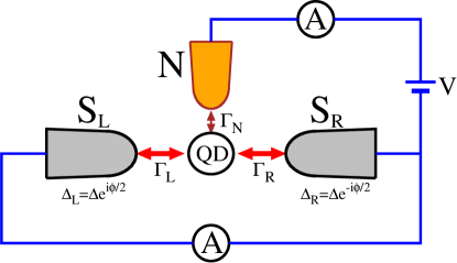
Figure 1: (Color online) Sketch of the three-terminal device, where the quantum dot (QD) is coupled between the normal (N) and two superconducting (S) leads. Phase difference $\phi$ in the Josephson loop affects the Kondo state originating from the spin-exchange interactions between the QD and N electrode.

In practical realizations of the N-QD-S and S-QD-S heterostructures the impurity levels can be varied by the gate potential, changing their even/odd occupancy De Franceschi et al. (2010) which triggers evolution of the in-gap states (affecting both their energies and spectral weights). Another important influence comes from the repulsive Coulomb interactions Bauer et al. (2007); Yamada et al. (2011). In-gap states may cross each other (at the Fermi energy) when energies of the singly occupied configurations $\left|\uparrow\right>$, $\left|\downarrow\right>$ coincide with one of the BCS-type superpositions $u_{d}\left|0\right>-v_{d}\left|\uparrow\downarrow\right>$ or $v_{d}\left|0\right>+u_{d}\left|\uparrow\downarrow\right>$ . In S-QD-S circuits this singlet-doublet quantum phase transition is responsible for a reversal of the DC Josephson current, so called “$0-\pi$ transition”, studied theoretically Matsuura (1977); *Glazman-1989; *Rozhkov-1999; *Yoshioka-2000; *Siano-2004; *Choi-2004; *Sellier-2005; *Novotny-2005; *Karrasch-2008; *Meng-2009; Žonda et al. (2015); *Zonda-2016; Wentzell et al. (2016) and in the last decade observed experimentally van Dam et al. (2006); *Cleuziou-2006; *Jorgensen-2007; *Eichler-2009; Maurand et al. (2012); *Delagrange-2015; *Delagrange-2016.

On the other hand, in N-QD-S heterostructures the singlet to doublet crossover is smooth Žitko et al. (2015); Jellinggaard et al. (2016) because the quasiparticle states appearing in the subgap energy region $|\omega|\leq\Delta$ acquire a finite broadening due to the hybridization with itinerant electrons of the normal lead. This crossover has also implications on the efficiency of the screening interactions responsible for the presence of the Kondo effect Maurand and Schönenberg (2013). The recent theoretical studies have indicated that upon approaching the crossover region from the doublet side the antiferromagnetic spin-exchange coupling is substantially enhanced, amplifying the Kondo effect that can appear in the subgap regime solely for the spinful (doublet) configuration Žitko et al. (2015); Wójcik and Weymann (2014); Domański et al. (2016). Although signatures of the subgap Kondo effect have been experimentally observed Deacon et al. (2010); Hübler et al. (2012); Chang et al. (2013); Lee et al. (2014) such an intriguing evolution in the doublet-singlet crossover region is still awaiting the systematic verification.

Inspired by Refs. Oguri and Tanaka (2012); Oguri et al. (2013); Kiršanskas et al. (2015) we consider here both the Josephson and Andreev circuits arranged in the Y-shape geometry depicted in Fig. 1. This three-terminal heterostructure would allow for a precise and phase-tunable experimental study of the singlet-doublet transition and its influence on the Kondo effect in the spirit of recent Refs. Delagrange et al. (2015, 2016). Phase difference $\phi$ between the left and right superconducting reservoirs induces DC Josephson current – its reversal can help to spot the $0-\pi$ crossover where the subgap quasibound states cross each other. The role of the subgap voltage $V$ applied between the normal electrode and Josephson circuit is twofold: It primarily induces the Andreev current, whose differential conductance can be used for determination of the Kondo temperature Domański et al. (2016), but it may also shift the impurity level.

Interacting QD coupled to the usual normal Fermi liquid develops the quasiparticle state at $\varepsilon_{d}$, its Coulomb satellite at $\varepsilon_{d}+U_{d}$ and, at low temperatures, the Kondo peak at zero energy (see the dashed blue line in Fig. 2). Broadening of the charge quasiparticle states is controlled by $\Gamma_{N}$, whereas the zero-energy peak depends on the effective exchange potential Schrieffer and Wolff (1966). Its half-width can be related to the characteristic Kondo scale $k_{B}T_{K}$ Haldane (1978); *Tsvelik-83. In our setup involving superconducting leads (Fig. 1) the QD spectrum is completely different. We illustrate the qualitative changes by the solid line in Fig. 2, obtained for the doublet ground state configuration at the particle-hole symmetric point ($\varepsilon_{d}=-U_{d}/2$) in the limit $\Delta\to\infty$. Instead of the charge peaks at $\pm U_{d}/2$ of the normal case we observe four Andreev quasibound states at $\pm[U_{d}/2\pm\Gamma_{S}\cos(\phi/2)]$ Barański and Domański (2013) coexisting with the zero-energy Kondo peak, which has, however, a substantially broadened width in comparison to the $\Gamma_{S}=0$ value Žitko et al. (2015); Domański et al. (2016). These effects are caused by interplay of the proximity effect induced by the couplings $\Gamma_{L,R}$ with the correlations due to $U_{d}$, and they depend on the coupling $\Gamma_{N}$ to the normal electrode Žitko et al. (2015).

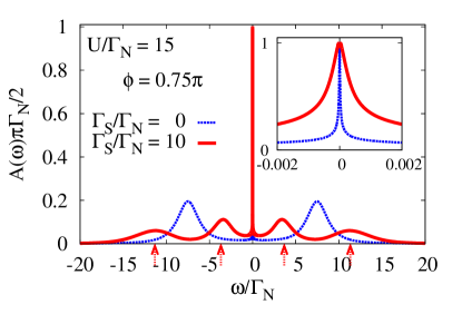
Figure 2: (Color online) Spectrum of the half-filled ($\varepsilon_{d}=-U_{d}/2$) QD obtained by the NRG calculations for $\Delta\to\infty$, $U_{d}/\Gamma_{N}=15$ assuming $\Gamma_{S}=0$ (dashed blue line) and $\Gamma_{S}/\Gamma_{N}=10$ (solid red line). Red dashed arrows indicate the energies of Andreev bound states in the limit $\Gamma_{N}\to 0$. Inset presents details of the low-energy (Kondo) region.

The subtle influence of the normal electrode has already been studied by König and coworkers Governale et al. (2008); *Futterer-2013 by means of the perturbative real-time diagrammatic expansion with respect to the hybridization terms. Their analysis has been next extended to the Kondo regime using the numerical renormalization group (NRG) calculations in the infinite gap $\Delta\to\infty$ limit Oguri and Tanaka (2012); Oguri et al. (2013) and/or for finite gap but just a single superconducting reservoir (i.e., no option of tuning the phase difference $\phi$) Žitko et al. (2015). Additional information has been recently obtained from the T-matrix studies of the classical and quantum spin impurity Kiršanskas et al. (2015), revealing the phase $\phi$ dependence of the subgap states — however, the employed classical-spin and perturbative quantum approximations do not address the Kondo effect.

Our work extends the previous studies of the subgap states Governale et al. (2008); *Futterer-2013; Oguri et al. (2013); Kiršanskas et al. (2015), focusing on the phase-tunable Kondo physics and its possible empirical observability. In what follows we explore the phase dependence of the Kondo effect, using: (i) perturbative treatment of the hybridization $V_{{\bf k}N}$ by the Schrieffer-Wolff transformation Schrieffer and Wolff (1966); Bravyi et al. (2011); Zamani et al. (2016) generalized to the superconducting Hamiltonian Domański et al. (2016), (ii) the self-consistent second order perturbative treatment of the Coulomb potential $U_{d}$ Žonda et al. (2015); *Zonda-2016, (iii) the NRG Bulla et al. (2008); Žitko et al. (2015); Žitko (2016), and QMC Gull et al. (2011); Luitz and Assaad (2010); *Luitz-2012 calculations. We determine the Kondo temperature for a wide range of parameters by a suitable combination of these methods and obtain its universal phase scaling $\mbox{{\rm ln}}T_{K}(\phi)\propto\mbox{{\rm cos}}^{2}\left(\phi/2\right)$.

The paper is organized as follows. In Sec. II, after introducing the model Hamiltonian in Sec. II.1, we present the four used theoretical methods — namely, the effective spin-exchange interaction via the generalized Schrieffer-Wolff transformation in Sec. II.2, second-order perturbation theory in $U_{d}$ in Sec. II.3, NRG in Sec. II.4, and QMC in Sec. II.5. We then analyze the obtained results for the spectral function (Sec. III), Josephson current (Sec. IV), and finally for the Andreev conductance in Sec. V. We summarize our study in Sec. VI.

II Model and methods

II.1 Microscopic formulation

Three-terminal system with the quantum dot depicted in Fig. 1 can be described by the Anderson model Hamiltonian

$$\hat{H} = \sum_{\sigma}\varepsilon_{d}\hat{d}_{\sigma}^{\dagger}\hat{d}_{\sigma}+U_{d}\hat{n}_{d\uparrow}\hat{n}_{d\downarrow}+\sum_{\beta}\hat{H}_{\beta}$$

$$+ \sum_{{\bf k},\sigma}\sum_{{\beta}}\left(V_{{\bf k}\beta}\;\hat{d}_{\sigma}^{\dagger}\hat{c}_{{\bf k}\sigma\beta}+V_{{\bf k}\beta}^{*}\hat{c}_{{\bf k}\sigma\beta}^{\dagger}\hat{d}_{\sigma}\right),$$

where the reservoirs $$\beta=N,L,R$$ of itinerant electrons are given by

$$\hat{H}_{N} = \sum_{{\bf k},\sigma}\xi_{{\bf k}N}\hat{c}_{{\bf k}\sigma N}^{\dagger}\hat{c}_{{\bf k}\sigma N},$$ (1b)

$$\hat{H}_{S} = \sum_{{\bf k},\sigma}\xi_{{\bf k}S}\hat{c}_{{\bf k}\sigma S}^{\dagger}\hat{c}_{{\bf k}\sigma S}$$

$$- \Delta\sum_{{\bf k}}\left(e^{i\phi_{S}}\hat{c}_{{\bf k}\uparrow S}^{\dagger}\hat{c}_{-{\bf k}\downarrow S}^{\dagger}+e^{-i\phi_{S}}\hat{c}_{-{\bf k}\downarrow S}\hat{c}_{{\bf k}\uparrow S}\right)$$

and $S=L,R$. We use the second quantization notation, in which $\hat{d}_{\sigma}^{({\dagger})}$ annihilates (creates) an electron with spin $\sigma$ at the QD energy level $\varepsilon_{d}$. As usually $\hat{n}_{d\sigma}=\hat{d}_{\sigma}^{\dagger}\hat{d}_{\sigma}$ stands for the number operator and $U_{d}$ is the repulsive Coulomb potential between opposite spin electrons. The QD is coupled to the mobile electrons of $\beta$ reservoir by the matrix elements $V_{{\bf k}\beta}$ and the energies $\xi_{{\bf k}\beta}=\varepsilon_{{\bf k}}-\mu_{\beta}$ are measured with respect to the chemical potentials $\mu_{\beta}$ ($\mu_{L}=\mu_{R}=0$), which can be detuned by the voltage $\mu_{N}=eV$. We assume that both superconductors are isotropic and are characterized by the complex order parameters $\Delta e^{i\phi_{S}}$.

Our major concern here are the states appearing in the low-energy subgap regime $|\omega|\leq\Delta$ therefore we can assume the couplings $\Gamma_{\beta}=2\pi\sum_{{\bf k}}|V_{{\bf k}\beta}|^{2}\;\delta(\omega\!-\!\xi_{{\bf k}\beta})$ to be constant. In realistic systems the Coulomb potential by far exceeds the superconducting gap $U_{d}\gg\Delta$ and, consequently, the outer Andreev states are pushed towards the band edges or even into the continuum Martín-Rodero and Levy Yeyati (2011); Kiršanskas et al. (2015). For this reason we shall disregard them from our considerations, which are primarily focused on the deep subgap regime. To simplify the formulas we focus on the symmetric couplings $\Gamma_{L}=\Gamma_{R}\equiv\Gamma_{S}/2$ of the Josephson loop which is phase biased by $\phi\equiv\phi_{L}-\phi_{R}$. Asymmetric coupling $\Gamma_{L}\neq\Gamma_{R}$ can be handled easily by the replacement $\cos(\phi/2)\to\sqrt{1-4\Gamma_{L}\Gamma_{R}\sin^{2}(\phi/2)/(\Gamma_{L}+\Gamma_{R})^{2}}$ Kadlecová et al. (2016). Our numerical calculations are mostly performed for the half-filled QD ($\varepsilon_{d}=-U_{d}/2$). In what follows we address: (i) emergence of the subgap Kondo state in the limit $k_{B}T_{K}\ll\Delta$, (ii) its evolution upon approaching the doublet to singlet crossover, and (iii) observable signatures of the phase-dependent Kondo effect in the transport properties.

II.2 Effective spin exchange interaction

To quantify analytically the phase dependence of the Kondo features we estimate the effective spin-exchange potential driven by the hybridization term $\hat{V}_{N}=\sum_{{\bf k},\sigma}\left(V_{{\bf k}N}\;\hat{d}_{\sigma}^{\dagger}\hat{c}_{{\bf k}\sigma N}+V_{{\bf k}N}^{*}\hat{c}_{{\bf k}\sigma N}^{\dagger}\hat{d}_{\sigma}\right)$ and the local Coulomb interaction $U_{d}\hat{n}_{d\uparrow}\hat{n}_{d\downarrow}$. This can be done rather straightforwardly in the SC atomic limit of very large gap $\Delta\to\infty$ by adopting the Schrieffer-Wolff approach Schrieffer and Wolff (1966); Bravyi et al. (2011); Zamani et al. (2016) to the effective Hamiltonian Tanaka et al. (2007a); Karrasch et al. (2008); Martín-Rodero and Levy Yeyati (2011); Oguri et al. (2013)

$$\hat{H_{\mathrm{eff}}} = \hat{H}_{N}+\hat{V}_{N}+\sum_{\sigma}\varepsilon_{d}\hat{d}_{\sigma}^{\dagger}\hat{d}_{\sigma}+U_{d}\hat{n}_{d\uparrow}\hat{n}_{d\downarrow}$$ (2)

$$- \Delta_{d}(\phi)\left(\hat{d}_{\uparrow}^{\dagger}\hat{d}_{\downarrow}^{\dagger}+\hat{d}_{\downarrow}\hat{d}_{\uparrow}\right).$$

with the real induced pairing potential $\Delta_{d}(\phi)\equiv\Gamma_{S}\cos(\phi/2).$ Apart from the explicit expression for $\Delta_{d}$ in terms of model parameters this Hamiltonian is identical to that of Ref. Domański et al. (2016), Eq. (2). We can therefore follow exactly the same extended Schrieffer-Wolff (SW) procedure eliminating perturbatively the hybridization term $\hat{V}_{N}$ from the Hamiltonian (2) by a canonical unitary transformation to obtain the spin-exchange interaction

$$\hat{H}_{\mathrm{exch}}=-\sum_{{\bf k},{\bf p}}J_{{\bf k,p}}(\phi)\;\;\hat{{\bf S}}_{d}\cdot\hat{{\bf S}}_{{\bf k}{\bf p}}$$ (3)

between the QD spin $\hat{{\bf S}}_{d}$ and the spins of the normal lead electrons $\hat{{\bf S}}_{{\bf k}{\bf p}}$. The coupling potential near the Fermi energy $J_{\mathrm{{\bf k_{F},}\mathbf{k_{F}}}}(\phi)$ is given by (compare with Eq. (19) of Ref. Domański et al. (2016))

$$J_{{\bf k}_{F},{\bf k}_{F}}(\phi)=\frac{U_{d}\left|V_{{\bf k}_{F}}\right|^{2}}{\varepsilon_{d}\left(\varepsilon_{d}+U_{d}\right)+\Delta_{d}^{2}(\phi)}$$ (4)

with $\phi$-dependent $\Delta_{d}(\phi)$ in the present case. The vanishing denominator of Eq. (4) $\varepsilon_{d}\left(\varepsilon_{d}+U_{d}\right)+\Delta_{d}^{2}(\phi_{c})=0$ defines the singlet-doublet transition point (if it exists for any $\phi_{c}\in(0,2\pi)$) Oguri et al. (2013)

$$\phi_{c}=2\arccos\frac{\sqrt{|\varepsilon_{d}|(\varepsilon_{d}+U_{d})}}{\Gamma_{S}}.$$ (5)

The ferromagnetic regime can be, however, completely disregarded, because it would have no effect on the BCS-type (spinless) configuration $u_{d}\left|0\right>-v_{d}\left|\downarrow\uparrow\right>$.

We can determine the effective Kondo temperature for the doublet (spinful) configuration using the well-known formula Haldane (1978); *Tsvelik-83 $T_{K}\propto\mbox{{\rm exp}}\left\{-1/\left[2\rho(\varepsilon_{F})J_{{\bf k}_{F}{\bf k}_{F}}\right]\right\}$, where $\rho(\varepsilon_{F}$) is the density of states of the normal lead at the Fermi level. We thus obtain

$$T_{K}(\phi)=\eta\;\frac{\sqrt{\Gamma_{N}U_{d}}}{2}\;{\rm exp}\!\left[\pi\;\frac{\varepsilon_{d}\left(\varepsilon_{d}+U_{d}\right)+\Delta_{d}^{2}(\phi)}{\Gamma_{N}U_{d}}\right]$$ (6)

with $\eta$ being of the order of unity (its specific value depending on the exact definition of $T_{K}$). Its comparison to the normal case corresponding to $\Gamma_{S}=0$ and hence $\Delta_{d}(\phi)=0$ yields the following phase scaling of the relative Kondo temperature

$$\ln\left(\frac{T_{K}}{T_{K}^{N}}\right)=\frac{\pi\;\Gamma_{S}^{2}}{\Gamma_{N}U_{d}}\;\cos^{2}\left(\frac{\phi}{2}\right)$$ (7)

valid in the doublet region $\cos^{2}({\phi}/{2})<|\varepsilon_{d}|(U_{d}+\varepsilon_{d})/\Gamma_{S}^{2}$ (equal to $(U_{d}/2\Gamma_{S})^{2}$ for the particle-hole symmetric case).

In experiments the value of the SC gap $\Delta$ is typically smaller or comparable to the other parameters such as $\Gamma_{S}$ and $U_{d}$. Thus, the above derivation cannot be directly used. Extension of the above Schrieffer-Wolff procedure to the finite-$\Delta$ case remains an open question, which is further complicated by the lack of the numerical support by NRG, which practically cannot handle the associated three-channel setup (see below in Sec. II.4). We wish to point out explicitly that the extension of the Schrieffer-Wolff procedure to the superconducting case by Salomaa Salomaa (1988) and its further application to the NS case Žitko et al. (2015) based on the perturbative treatment of both $\Gamma_{N}$ and $\Gamma_{S}$ is not sufficient for our present purpose of determining the phase-dependent change of the Kondo temperature. Due to its perturbative nature in $\Gamma_{S}$ it fails completely to capture the effect of the SC lead(s) on the exchange coupling between the localized spin and the normal lead electrons, cf. Eq. (B19) in Ref. Žitko et al. (2015). Our result (4), on the contrary, contains the effects of the SC leads in a fully resummed fashion via the $\Delta_{d}^{2}(\phi)$ term in the denominator. It is not currently clear to us how to achieve such a nonperturbative result in the finite-$\Delta$ case, where the SC leads cannot be so straightforwardly incorporated into the effective Hamiltonian (2).

II.3 Perturbative treatment in $U_{d}$

It has been recently shown for the S-QD-S Žonda et al. (2015); *Zonda-2016 and N-QD-S Domański et al. (2016) junctions, that some of the NRG results can be reproduced using the self-consistent perturbative treatment of the interaction $U_{d}\hat{n}_{d\downarrow}\hat{n}_{d\uparrow}$. This fact encouraged us to apply the same technique to our three-terminal system in Fig. 1. For treating the mixed particle and hole degrees of freedom we have to formulate the diagrammatic expansions for the (real-time) matrix Green’s function ${{\mbox{\boldmath{$G$}}}}(t,t^{\prime})\!=\!\langle\!\langle\hat{\Psi}_{d}(t);\hat{\Psi}_{d}^{\dagger}(t^{\prime})\rangle\!\rangle$ in the Nambu representation, where $\hat{\Psi}_{d}\equiv(\hat{d}_{\uparrow},\hat{d}_{\downarrow}^{\dagger})^{T}$. Its Fourier transform obeys the Dyson equation

$${{\mbox{\boldmath{$G$}}}}^{-1}(\omega)=\left(\begin{array}[]{cc}\omega\!-\!\varepsilon_{d}&0\\ 0&\omega\!+\!\varepsilon_{d}\end{array}\right)-{{\mbox{\boldmath{$\Sigma$}}}}(\omega),$$ (10)

where the self-energy ${{\mbox{\boldmath{$\Sigma$}}}}(\omega)$ accounts for the three external reservoirs and for the correlation effects due to $U_{d}$. In the absence of the correlations the self-energy ${\mbox{\boldmath{$\Sigma$}}}^{0}(\omega)\equiv\left.{\mbox{\boldmath{$\Sigma$}}}(\omega)\right|_{U_{d}=0}$ can be obtained exactly. In the wide band limit it is given by the following formula Bauer et al. (2007); Yamada et al. (2011)

$${\mbox{\boldmath{$\Sigma$}}}^{0}(\omega) = -\;\frac{i\Gamma_{N}}{2}\;\left(\begin{array}[]{cc}1&0\\ 0&1\end{array}\right)-\Gamma_{S}\mbox{{\rm cos}}\left(\frac{\phi}{2}\right)\left(\begin{array}[]{cc}1&\frac{\Delta}{\omega}\\ \frac{\Delta}{\omega}&1\end{array}\right)$$ (15)

$$\times \left\{\begin{array}[]{ll}\frac{\omega}{\sqrt{\Delta^{2}-\omega^{2}}}&\mbox{{\rm for }}|\omega|<\Delta\\ \frac{i\;|\omega|}{\sqrt{\omega^{2}-\Delta^{2}}}&\mbox{{\rm for }}|\omega|>\Delta\end{array}\right..$$ (18)

Equation (18) describes the induced on-dot pairing via the off-diagonal term proportional to $\Gamma_{S}$ and the finite life-time effects which enter through the imaginary parts of the self-energy ${\mbox{\boldmath{$\Sigma$}}}^{0}(\omega)$. Extending our previous studies Domański et al. (2016); Žonda et al. (2015); *Zonda-2016 to the present three-terminal heterostructure (Fig. 1) we express the full ${\mbox{\boldmath{$\Sigma$}}}(\omega)$ using the second-order perturbation theory (SOPT) Žonda et al. (2015); *Zonda-2016; Vecino et al. (2003)

$${{\mbox{\boldmath{$\Sigma$}}}}_{11}(\omega) = {{\mbox{\boldmath{$\Sigma$}}}}_{11}^{0}(\omega)+U_{d}\langle\hat{d}_{\downarrow}^{\dagger}\hat{d}_{\downarrow}\rangle$$

$$+ U_{d}^{2}\int\limits_{-\infty}^{\infty}{\frac{-\frac{1}{\pi}\mbox{{\rm Im}}{{{\mbox{\boldmath{$\Sigma$}}}}_{11}^{(2)}(\omega^{\prime})}}{{\omega-\omega^{\prime}+i0^{+}}}d\omega^{\prime}},$$

$${{\mbox{\boldmath{$\Sigma$}}}}_{12}(\omega) = {{\mbox{\boldmath{$\Sigma$}}}}_{12}^{0}(\omega)+U_{d}\langle\hat{d}_{\downarrow}\hat{d}_{\uparrow}\rangle$$

$$- U_{d}^{2}\int\limits_{-\infty}^{\infty}{\frac{-\frac{1}{\pi}\mbox{{\rm Im}}{{{\mbox{\boldmath{$\Sigma$}}}}_{12}^{(2)}(\omega^{\prime})}}{{\omega-\omega^{\prime}+i0^{+}}}d\omega^{\prime}}.$$

The imaginary parts of the second-order contributions $${{\mbox{\boldmath{$\Sigma$}}}}_{ij}^{(2)}(\omega)$$ are expressed by the following convolutions

$$-\frac{1}{\pi}\mbox{{\rm Im}}{{\mbox{\boldmath{$\Sigma$}}}}_{11(12)}^{(2)}(\omega) = \int\limits_{-\infty}^{\infty}\left[{{\mbox{\boldmath{$\Pi$}}}}_{1}(\omega+\omega^{\prime})\rho_{22(12)}^{+}(\omega^{\prime})\right.$$ (19c)

$$+ \left.{{\mbox{\boldmath{$\Pi$}}}}_{2}(\omega+\omega^{\prime})\rho_{22(12)}^{-}(\omega^{\prime})\right]\;d\omega^{\prime},$$

$${{\mbox{\boldmath{$\Pi$}}}}_{1(2)}(\omega) = \int\limits_{-\infty}^{\infty}\left[\rho_{11}^{-(+)}(\omega^{\prime})\rho_{22}^{-(+)}(\omega-\omega^{\prime})\right.$$ (19d)

$$- \left.\rho_{12}^{-(+)}(\omega^{\prime})\rho_{21}^{-(+)}(\omega-\omega^{\prime})\right]\;d\omega^{\prime},$$

where the auxiliary functions $\rho_{ij}^{\pm}(\omega)\equiv-\mathrm{Im}\,{{\mbox{\boldmath{$G$}}}}_{ij}^{\mathrm{H}F}(\omega\!+\!i0^{+})f(\pm\omega)/\pi$ (with the standard Fermi-Dirac distribution $f(\omega)\equiv 1/\left[1+\mbox{{\rm exp}}\left(\omega/k_{B}T\right)\right]$) denote the occupancies obtained at the Hartree-Fock approximation level $\sum_{\sigma}\varepsilon_{d}\hat{d}_{\sigma}^{\dagger}\hat{d}_{\sigma}+U_{d}\;\hat{n}_{d\uparrow}\hat{n}_{d\downarrow}\rightarrow\sum\limits_{\sigma}{\left({\varepsilon_{d}+U_{d}\langle\hat{n}_{d-\sigma}\rangle}\right)\hat{n}_{d\sigma}}+U_{d}(\langle\hat{d}_{\downarrow}\hat{d}_{\uparrow}\rangle\hat{d}_{\uparrow}^{\dagger}\hat{d}_{\downarrow}^{\dagger}+\mbox{{\rm h.c.}})$.

II.4 NRG

The most reliable (unbiased) information about the relationship between the electron correlations and induced pairing can be obtained within a nonperturbative scheme of the numerical renormalization group (NRG) technique Bulla et al. (2008). We have performed NRG calculations using the open source code NRG LJUBLJANA Žitko and Pruschke (2009); *Ljubljana-code. For the infinite SC gap $\Delta\to\infty$ the NRG reduces to a single channel problem Oguri et al. (2013); Tanaka et al. (2007b), where we have set the logarithmic discretization parameter $\Lambda=1.9$. The case of finite $\Delta$ is in general a three-channel problem and trustworthy NRG calculations for the Anderson model with three channels are extremely demanding. Fortunately, in the special case of $\phi=0$ one can effectively reduce this problem to two channels. The NRG data for this case have been calculated with $\Lambda=4$, as is common for such double-channel models.

II.5 CT-HYB

We have also utilized continuous-time quantum Monte-Carlo (CT-QMC) calculations Gull et al. (2011) in order to study the effect of finite temperature on the system and to obtain results in regions, where NRG is ineffective. Since Hamiltonian (1) does not conserve the electron number, we perform the canonical particle-hole transformation

$$\hat{d}_{\uparrow}^{{\dagger}}\rightarrow\tilde{d}_{\uparrow}^{{\dagger}},\quad\hat{d}_{\downarrow}^{{\dagger}}\rightarrow\tilde{d}_{\downarrow}^{\phantom{{\dagger}}},\quad\hat{c}_{\mathbf{k},\uparrow,\beta}^{{\dagger}}\rightarrow\tilde{c}_{\mathbf{k},\uparrow,\beta}^{{\dagger}},\quad\hat{c}_{\mathbf{k},\downarrow,\beta}^{{\dagger}}\rightarrow\tilde{c}_{\mathbf{-k},\downarrow,\beta}^{\phantom{{\dagger}}}$$ (20)

which was already used by Luitz and Assaad Luitz and Assaad (2010) to include superconductivity in the CT-QMC calculations. The new quasiparticles described by $\tilde{c}$ and $\tilde{d}$ operators are identical to electrons in the spin-up sector and to holes in the spin-down sector. This transformation maps our system to a one-band Anderson model with attractive interaction $-U_{d}$ and local energy term $\varepsilon_{d}(\tilde{n}_{\uparrow}-\tilde{n}_{\downarrow})$, where $\tilde{n}_{\sigma}=\tilde{d}_{\sigma}^{{\dagger}}\tilde{d}_{\sigma}^{\phantom{{\dagger}}}$.

We use the TRIQS hybridization-expansion continuous-time (CT-HYB) quantum Monte Carlo solver Seth et al. (2016) based on the TRIQS libraries Parcollet et al. (2015). We consider a flat band in the leads of finite width $D=20\Gamma_{S}$. The induced gap $\Delta_{I}$ and Josephson current $I_{J}$ are obtained from the anomalous part of the imaginary-time Green’s function Luitz and Assaad (2010); *Luitz-2012.

III Spectral function and the Kondo scale

Phase evolution of the (diagonal) spectral function $A(\omega)\equiv-\mbox{{\rm Im}}{{\mbox{\boldmath{$G$}}}}_{11}(\omega+i0^{+})/\pi$ obtained by the second order perturbation theory (SOPT; Eqs. (19)) and compared with the NRG results is displayed in Fig. 3. The panels correspond to the half-filled QD case ($\varepsilon_{d}=-U_{d}/2$) in the large-gap regime $\Delta\to\infty$ with $\Gamma_{N}=\Gamma_{S}/2$ and different Coulomb potentials, as indicated. In both cases we see an excellent agreement between the SOPT and NRG data with some quantitative differences noticeable only in the lower panel for intermediate $\phi$’s.

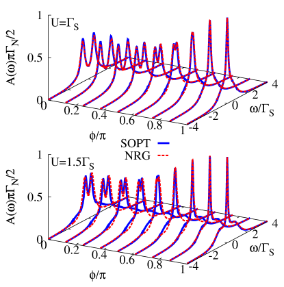
Figure 3: (Color online) Phase dependence of the diagonal spectral function $A(\omega)$ of the half-filled QD in the large-gap limit $\Delta\to\infty$ obtained by SOPT (blue solid lines) and NRG calculations (red dashed curves). Results are presented for $\Gamma_{N}/\Gamma_{S}=0.5$ and two values of the Coulomb potential $U_{d}/\Gamma_{S}=1$ (top panel) and $U_{d}/\Gamma_{S}=1.5$ (bottom panel).

For both values of the Coulomb potential $U_{d}$, the subgap electronic spectrum shows either the absence (for the spinless BCS-type configuration, close to the $0$ phase for small $\phi$’s) or presence (for the spinful doublet state, close to $\pi$ phase for $\phi\gtrsim\phi_{c}=2\arccos\left(U_{d}/2\Gamma_{S}\right)$ given by Eq. (5)) of the central Kondo-like peak around zero frequency. Such a phase evolution we assign to the efficiency or lack of the screening interactions.

Figure 4 shows the phase-dependent Kondo temperature determined as the half-width at half maximum (HWHM) of the zero-energy peak by the NRG and SOPT and compared to the generalized Schrieffer-Wolff prediction (7). We observe a very good correspondence between NRG and SOPT for small enough $U_{d}$ (panel b) and between NRG and SW for larger values of $U_{d}$ (panels a and c). The deviations observed between the NRG data and SW prediction occur close to the $0-\pi$ crossover where the central Kondo-like peak merges with the broadened Andreev states and the identification of the Kondo scale from the HWHM is no longer reliable. Furthermore, the effective exchange coupling (4) diverges at the $0-\pi$ transition where the perturbative SW approach necessarily breaks down and, thus, the SW prediction close to the transition stops working. Nonperturbative treatment beyond the simple SW approach based on the flow equations (corrected version of Ref. Zapalska and Domański (2014)) shows sharp but smooth features at the transition point; this issue is, however, beyond our current scope and the refined results will be published elsewhere. For the largest value of $U_{d}$ in the particle-hole symmetric case (black curves in panel a) when the system is close to the $\pi$ phase for all $\phi$’s the agreement between the two methods is nearly perfect.

In general, the trend extracted from all the available data confirms the enhancement of $T_{K}$ (i.e., broadening of the Kondo-like peak with respect to the normal case as seen already in the inset of Fig. 2) upon approaching the singlet state from the doublet side. For sufficiently large values of $U_{d}$ the Kondo scale enhancement follows quite well the analytical formula (7) above $\phi_{c}$ (5). The logarithm of the enhancement is proportional to $\cos^{2}(\phi/2)$ with the proportionality constant inversely decaying with increasing $U_{d}$ — for the strong Coulomb interaction $U_{d}$ the relative value of the Kondo scale hardly changes with respect to $\phi$ because the correlations dominate over the induced electron pairing. For the opposite case of relatively small $U_{d}$, the Kondo state survives only when the Josephson phase $\phi$ is nearby $\pi$ (i.e., $\phi\gtrsim\phi_{c}$), where the quantum interference between superconducting reservoirs is destructive.

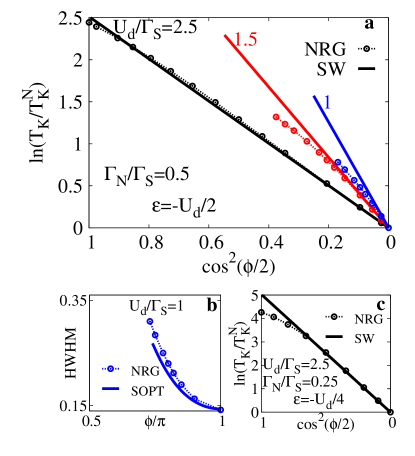
Figure 4: (Color online) (a) Phase dependence of the Kondo temperature $T_{K}$ obtained by NRG for $\Gamma_{N}/\Gamma_{S}=0.5$ and several potentials $U_{d}/\Gamma_{S}$ as indicated (dotted lines with bullets) and compared to the generalized Schrieffer-Wolff prediction (7) (full lines) ending at the transition point determined by Eq. (5). (b) Comparison of the absolute HWHM from the NRG and SOPT for relatively small $U_{d}=\Gamma_{S}$. (c) Analogously to panel a for the large $U_{d}=2.5\Gamma_{S}$ and smaller normal coupling $\Gamma_{N}=\Gamma_{S}/4$ but away from the half-filling ($\varepsilon_{d}=-U_{d}/4$). In all panels we use the large-gap limit $\Delta\to\infty$ and in panels a and c the $T_{K}$ is normalized to $T_{K}^{N}$ corresponding to $\Gamma_{S}=0$ (i.e., in the absence of the proximity effect).

The above conclusions are based on the results in the large-gap limit $\Delta\to\infty$ where the NRG works reliably. However, as already mentioned this limit is not experimentally realistic and one may wonder whether these statements do survive also for finite $\Delta$ cases. Unfortunately, the case of simultaneously finite $\Delta$ and $\phi$ is practically very difficult to handle by NRG and we must thus resort to an approximative treatment based on SOPT. As seen in Fig. 4, panel b SOPT and NRG yield comparable results and this encourages us to address the finite-$\Delta$ case by SOPT with results summarized in Fig. 5. The two panels describe (a) the large-gap $\Delta\to\infty$ case corresponding to the panel a of Fig. 4 and (b) fairly realistic finite $\Delta=\Gamma_{S}$ case at half-filling for the same set of $U_{d}/\Gamma_{N}$ ratios as in panel a. In both cases we do observe the universal linear behavior $\ln T_{K}\propto\cos^{2}(\phi/2)$ of the logarithm of the Kondo scale.

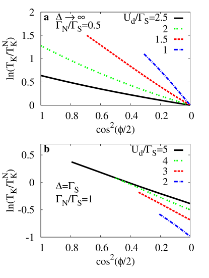
Figure 5: (Color online) Universal phase dependence $\ln T_{K}\propto\cos^{2}(\phi/2)$ of the normalized Kondo temperature $T_{K}$ obtained by the SOPT at half-filling for several $U_{d}/\Gamma_{N}$ values and large (a) and finite (b) gap.

Nevertheless, it is at place to mention several problematic aspects of this finding here. First, although the logarithm of the Kondo scale is proportional to $\cos^{2}(\phi/2)$ and the proportionality coefficient correctly decreases with increasing $U_{d}$, its value is not captured quantitatively precisely as can be seen by comparing the black lines (corresponding to $U_{d}/\Gamma_{S}=2.5$) in panels a of Figs. 4 and 5 — they should be identical but they are clearly not. This is not so surprising as this case corresponds to a rather large interaction value $U_{d}=5\Gamma_{N}$ where the SOPT, being a simple perturbation scheme, is not expected to yield very reliable results. For the smaller values of $U_{d}$ our SOPT findings should be even quantitatively correct as shown in panel b of Fig. 4. However, for such small values of the interaction, the central peak in the spectral function cannot be attributed to a true Kondo effect, rather to its weak coupling precursor. Despite all these objections we still believe that the qualitative conclusions drawn from the SOPT results, which confirm the universal phase dependence of the Kondo scale even for finite SC gap, are valid.

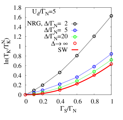
Figure 6: (Color online) SC-induced enhancement of the Kondo temperature at $\phi=0$ calculated by NRG as a function of $\Gamma_{S}$ for several finite values of the gap $\Delta$. The bottom curve corresponds to the infinite-gap limit and is perfectly determined by the SW formula (7).

Finally, we address the issue mentioned at the end of the Schrieffer-Wolff section II.2, namely, the effect of finite value of the SC gap $\Delta$ on the enhancement of the Kondo scale and its relation to the infinite-$\Delta$ limit. To obtain quantitatively reliable results we resort to the NRG calculations, which can be for finite $\Delta$ performed only for $\phi=0$ (see above). We plot the SC-enhanced Kondo temperature as a function of the coupling to the superconducting leads $\Gamma_{S}$ for several values of $\Delta$ in Fig. 6. The parameter values are chosen such that there is no $0-\pi$ transition in the whole range of $\phi$’s and the system is close to the $\pi$ phase even for $\phi=0$, where we evaluate the spectral function and read off the Kondo scale. We see that the enhancement gets even more pronounced with decreasing $\Delta$ (within reasonable limits — we always work in the regime where the Kondo peak is well inside the SC gap, i.e., $T_{K}\ll\Delta$). The values of $\Delta$ comparable to $\Gamma_{S}$ (corresponding to the topmost curve in Fig. 6) are experimentally fully justified, but we have no analytical theory for them, unlike in the $\Delta\to\infty$ case where the SW expression (7) pierces the NRG data. This remains an interesting and experimentally relevant open question.

IV Josephson current

For complete analysis of the three-terminal nanostructure we now address the Josephson loop. The DC supercurrent is known to deviate from the usual first Josephson law $I_{J}(\phi)=I_{c}\sin{\phi}$ nearby the singlet-doublet transition. The quantum phase transition (or crossover) reverses the Josephson current $I_{J}(\phi)$, and such a “$0-\pi$ transition” is due to the parity change of the induced electron pairing $\langle\hat{d}_{\downarrow}\hat{d}_{\uparrow}\rangle$. It can be practically achieved by tuning either the gate potential van Dam et al. (2006); *Cleuziou-2006; *Jorgensen-2007; *Eichler-2009, the superconducting phase Maurand et al. (2012); *Delagrange-2015; *Delagrange-2016 or magnetic field Wentzell et al. (2016).

The charge flow from the superconducting $L$ electrode to the QD can be derived using the Heisenberg equation of motion $I_{L}(\phi)=e\frac{d}{dt}\sum_{{\bf k},\sigma}\langle\hat{c}_{{\bf k}\sigma L}^{\dagger}\hat{c}_{{\bf k}\sigma L}\rangle=\frac{e}{i\hbar}\sum_{{\bf k},\sigma}\big{\langle}[\hat{c}_{{\bf k}\sigma L}^{\dagger}\hat{c}_{{\bf k}\sigma L},\hat{H}]\big{\rangle}$. It can be formally expressed by the anomalous Green’s function Žonda et al. (2015); *Zonda-2016

$$I_{L}(\phi)=\frac{2e}{\hbar\beta}\sum_{\omega_{n}}\frac{\Gamma_{S}\Delta}{\sqrt{\Delta^{2}+\omega_{n}^{2}}}\Im\left[{\mbox{\boldmath{$G$}}}_{12}(i\omega_{n})e^{i\phi/2}\right],$$ (21)

where $\omega_{n}=(2n+1)\pi\beta^{-1}$ are the fermionic Matsubara frequencies. We have previously shown Žonda et al. (2015); *Zonda-2016 that (21) satisfies the charge conservation $I_{L}(\phi)=-I_{R}(\phi)$ and is fully consistent with an alternative derivation of the Josephson current from the phase derivative of the free energy. In what follows we thus treat the DC Josephson current as $I_{J}(\phi)\equiv I_{L}(\phi)$. Let us remark, that in the infinite-gap limit $\Delta\rightarrow\infty$ Eq. (21) simplifies to Oguri et al. (2013)

$$I_{J}(\phi)=\frac{2e\Gamma_{S}}{\hbar}\;|\langle\hat{d}_{\downarrow}\hat{d}_{\uparrow}\rangle|\;\sin\left(\phi-\theta_{d}\right),$$ (22)

where $\theta_{d}=0$ or $\pi$ is the phase of the induced pairing $\langle\hat{d}_{\downarrow}\hat{d}_{\uparrow}\rangle=|\langle\hat{d}_{\downarrow}\hat{d}_{\uparrow}\rangle|\;e^{i\theta_{d}}$. Expression (22) explicitly implies the Josephson current reversal upon changing the parity $\theta_{d}$ between $0$ and $\pi$, which occurs at the singlet-doublet quantum phase transition van Dam et al. (2006); *Cleuziou-2006; *Jorgensen-2007; *Eichler-2009; Maurand et al. (2012); *Delagrange-2015; *Delagrange-2016.

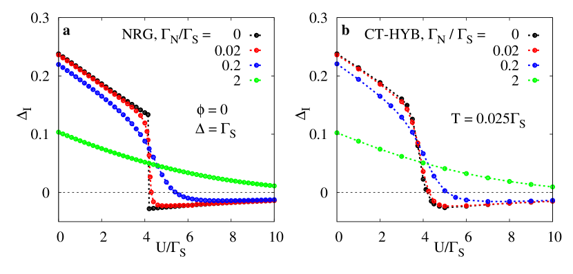
Figure 7: (Color online) Induced on-dot pairing $\Delta_{I}=\langle\hat{d}_{\downarrow}\hat{d}_{\uparrow}\rangle$ as a function of the interaction $U_{d}$ calculated for finite gap $\Delta=\Gamma_{S}$ and $\phi=0$ for several values of the normal electrode coupling $\Gamma_{N}$. (a) NRG results for T=0. (b) CT-HYB results for $T=0.025\Gamma_{S}$. QMC error bars are smaller than the symbol size.

In our three-terminal structure (Fig. 1) the metallic lead gives rise to a finite broadening of the subgap states, therefore the singlet evolves to doublet (and vice versa) in a continuous manner. This continuous crossover has already been discussed by Oguri et al. Oguri et al. (2013) for the superconducting atomic limit $\Delta\rightarrow\infty$. Here we extend the approach to the more realistic situations corresponding to finite SC gap $\Delta<\infty$ and nonzero temperature $T>0$.

Since the interplay of pairing and correlations affects the Josephson current indirectly via the pair correlation $\Delta_{I}\equiv\langle\hat{d}_{\downarrow}\hat{d}_{\uparrow}\rangle$ we first consider its variation as a function of the interaction strength $U_{d}$. Figure 7 shows the NRG (a) and CT-HYB (b) results obtained for representative couplings $\Gamma_{N}$, as indicated. In the absence of the normal lead ($\Gamma_{N}=0$) the induced pairing $\Delta_{I}$ changes abruptly at the quantum phase transition where the parity $\theta_{d}$ evolves from $0$ to $\pi$. Under such circumstances the $0-\pi$ transition in S-QD-S junctions is manifested by the sharp sign change of $I_{J}(\phi)$ van Dam et al. (2006); *Cleuziou-2006; *Jorgensen-2007; *Eichler-2009; Maurand et al. (2012); *Delagrange-2015; *Delagrange-2016 (theoretically a discontinuity at zero temperature $T=0$). For either finite couplings $\Gamma_{N}$ or finite temperature $T$ the induced pairing $\Delta_{I}$ continuously changes from the positive to negative values. Let us remark that the previous study Oguri et al. (2013) of the infinite-gap limit $\Delta\to\infty$ has not shown the negative values of $\Delta_{I}$. On the other hand, for sufficiently strong couplings $\Gamma_{N}$ the broadening of Andreev/Shiba states is so large that they are no longer distinguishable (spectroscopically they are seen as one broad structure). For this reason the induced pairing $\Delta_{I}$ monotonously decreases with respect to $U_{d}$ as seen in the behavior for the large value $\Gamma_{N}=2\Gamma_{S}$.

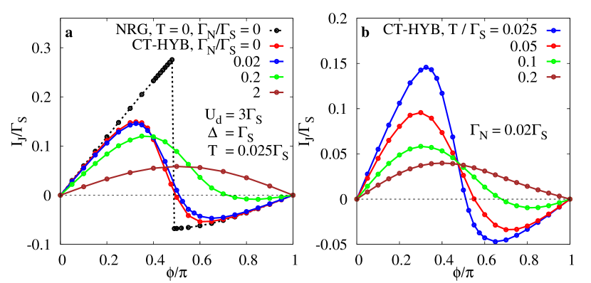
Figure 8: (Color online) Phase dependence of the DC Josephson current obtained from CT-HYB for $\Delta=\Gamma_{S}$ and $U_{d}=3\Gamma_{S}$ for fixed temperature $T=0.025\Gamma_{S}$ and changing $\Gamma_{N}$ (a) and fixed normal coupling $\Gamma_{N}=0.02\Gamma_{S}$ and varying temperature (b) as indicated. In the left panel a we included for $\Gamma_{N}=0$ the zero-temperature NRG results for comparison. QMC error bars are smaller than the symbol size.

Practical observability of the effects discussed above can be done by measuring the phase dependence of Josephson current. In Fig. 8 we plot the results (for $U=3\Gamma_{S}$ and $\Delta=\Gamma_{S}$) of evaluating Eq. (21) by CT-HYB analogously to Refs. Luitz and Assaad (2010); *Luitz-2012, since NRG is very inefficient in this situation (finite $\Delta$ and nonzero $\phi$ and $\Gamma_{N}$ implying a three-channel problem, see above). The results shown in the left panel a were obtained at fixed temperature $T=0.025\Gamma_{S}$. We included the available zero-temperature NRG data for $\Gamma_{N}=0$. Comparing the CT-HYB results with NRG shows that the chosen temperature used in CT-HYB is low enough to provide a reasonable value of critical $\phi_{c}$ for which the current changes sign. This point is pushed to higher values of $\phi$ with increasing $\Gamma_{N}$ and for high enough values of $\Gamma_{N}$ the region of the negative current ($\pi$ phase) is no longer present. Similar behavior is obtained by changing the temperature for a fixed value of $\Gamma_{N}$ in the right panel b . This indicates that indeed the normal coupling $\Gamma_{N}$ and temperature have qualitatively the same effect on the system — they both lead to the broadening of the Andreev/Shiba states and to vanishing of the $\pi$ phase.

However, this qualitative statement cannot be extended to quantitative predictions as we demonstrate in Fig. 9, where we try to model a finite $\Gamma_{N}$ by an effective temperature. More precisely, we attempt to mutually match two curves: one with very small $T$ and finite $\Gamma_{N}$ (red line) and the other with very small $\Gamma_{N}$ and finite effective temperature $T_{\mathrm{eff}}$ (blue and green curves). As can be seen from the figure, this attempt fails — we can fit either the small- or high-$\phi$ parts of the current-phase relations with various effective temperatures, but we cannot find a single effective temperature which would cover the whole phase range. Thus, the correspondence between the finite normal-lead coupling $\Gamma_{N}$ and temperature is only a vague qualitative analogy which should be used with much care.

Unfortunately, the phase-dependent Josephson current does not indicate directly any features that could be strictly assigned to the Kondo effect. We hence think that the Josephson loop of the three-terminal structure would be useful merely for spotting the singlet-doublet crossover region, where the Andreev differential conductance should reveal the characteristic zero-bias enhancement. Charge transport through the Andreev loop would then allow for precise measurement of the phase-tunable Kondo temperature as we now demonstrate.

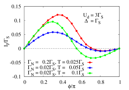
Figure 9: (Color online) Comparison between the effects of finite normal-lead coupling $\Gamma_{N}$ and temperature $T$. Failure to fit the finite-$\Gamma_{N}$ (red) curve with finite-temperature curve(s) (green & blue) demonstrates the nonexistence of a quantitative effective-temperature description of the normal lead influence (at least) on the Josephson transport.

V Andreev conductance

Empirical evaluation of the phase-controlled Kondo temperature can be carried out by the charge transport in the N-QD-S branch of our setup. Under general nonequilibrium conditions the current is given by the lesser Green’s function which should be determined from the Keldysh technique. However, for deeply subgap voltages $|V|\ll\Delta/e$ (of interest for our study of the subgap Kondo effect) the current can be expressed by the Landauer-Büttiker formula Fazio and Raimondi (1998); *Krawiec-2004

$$I_{A}(V)=\frac{2e}{h}\int\!\!d\omega\;T_{A}(\omega)\left[f(\omega\!-\!eV)\!-\!f(\omega\!+\!eV)\right].$$ (23)

This anomalous current is transmitted via the Andreev mechanism in which electrons from the conducting (N) reservoir are scattered into holes back to the same electrode, producing the Cooper pairs in superconducting (S) lead with the transmittance $T_{A}(\omega)\equiv\Gamma_{N}^{2}\left|{\mbox{\boldmath{$G$}}}_{12}(\omega+i0^{+})\right|^{2}$ which can be regarded as a quantitative measure of the induced on-dot pairing. Its maximal unitary value is achieved for the BCS-type ground state configurations when $eV$ coincides with the subgap Andreev/Shiba quasiparticle energies Barański and Domański (2013). Nevertheless, also for the (spinful) doublet configuration there is some contribution from the Andreev transport at least nearby the doublet-singlet crossover Domański et al. (2016). We suggest this particular feature for probing the phase-dependent Kondo temperature.

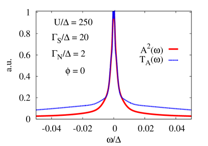
Figure 10: (Color online) Comparison between the square of the diagonal spectral function $A(\omega)$ of Sec. III and the Andreev transmittance $T_{A}(\omega)$ showing their identical zero-frequency-peak width which can be related to the Kondo scale.

To justify this proposal we first demonstrate that both the Andreev transmittance $T_{A}(\omega)$ and the diagonal spectral function $A(\omega)$ studied in detail in Sec. III are governed by the very same low-energy scale, i.e., the Kondo scale $T_{K}$. This means that the measurable width of the differential Andreev conductance $G_{A}(V)\equiv dI_{A}(V)/dV$ peak at $V=0$ can be related to the Kondo scale $T_{K}$ theoretically studied in Sec. III and, therefore, our theoretical predictions can be experimentally verified. At sufficiently low temperature the Andreev conductance $G_{A}(V)$ in terms of the conductance quantum $2e^{2}/h$ is equal to twice the Andreev transmittance, $G_{A}(V)=4e^{2}/h\,T_{A}(eV)$, and we thus just consider the two quantities interchangeably.

Figure 10 shows the (normalized) Andreev transmittance $T_{A}(\omega)$ and square of the spectral function $A(\omega)$ calculated by the NRG for a given set of parameters corresponding to the $\pi$ phase with a well-developed Kondo peak. We can clearly see that around $\omega=0$ both quantities overlap, which proves that the zero-frequency (Kondo) peaks are determined by a single scale which can be easily related to the Kondo scale studied in Sec. III. Technically, the Andreev transmittance is given as the square of the off-diagonal component of Green’s function (10) and that is the reason why it should be compared with the square of the diagonal spectral function which is determined by the diagonal part of Green’s function (10). This just means that the whole (matrix) Green’s function is governed by the single low-energy scale emerging as a complex zero point of the Green’s function determinant, cf. Refs. Žonda et al. (2015); *Zonda-2016.

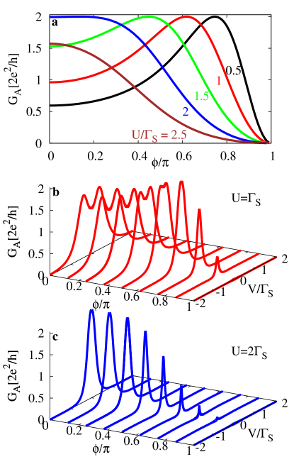
Figure 11: (Color online) (a) Phase dependence of the zero-bias Andreev conductance $G_{A}(V=0)$ in the infinite-gap limit $\Delta\to\infty$ for $\Gamma_{N}/\Gamma_{S}=0.5$ and several values of the Coulomb potential $U_{d}$ as indicated. (b) and (c) Differential Andreev conductance $G_{A}(V)$ as a function of the normal lead potential $V$ in the subgap regime corresponding to two values of the Coulomb interaction $U_{d}$ from the top panel a. All the results were obtained by NRG calculations.

In Fig. 11 we plot the phase dependence of the linear Andreev conductance $G_{A}(V=0)$ (panel a) as well as the finite-bias differential Andreev conductance $G_{A}(V)$ corresponding to two values of the Coulomb interaction $U_{d}=\Gamma_{S}$ (panel b) and $U_{d}=2\Gamma_{S}$ (panel c) from the panel a. Thus the corresponding curves in panel a are given as cuts $V=0$ of the graphs in the lower panels. Panel b depicts a situation with the $0-\pi$ crossover realized for an intermediate value of $\phi_{c}$ while in panel c the system always stays in the $\pi$ phase regardless of the value of $\phi\in(0,\pi)$. In the first situation (panel b), at small phase difference $\phi$ the system is in the BCS-type (singlet) configuration, we hence observe two maxima with the maximal conductance $G_{A}(V)=4e^{2}/h$. They appear at such voltage $eV$, which corresponds to the quasiparticle (Andreev/Shiba states) energies. Upon increasing the phase $\phi$ these maxima gradually merge at the critical phase $\phi_{c}$ where the linear Andreev conductance reaches its maximal value $4e^{2}/h$. At such a crossing point the ground state changes its configuration and the system enters the (spinful) doublet state Oguri et al. (2013). In that state the induced on-dot pairing is no longer efficient and, therefore, the Andreev conductance is suppressed. In the vicinity of such a singlet-doublet transition, from the doublet side, there appears the characteristic phase-dependent zero-bias enhancement due to the Kondo effect. The lower panel c for a stronger interacting case does not exhibit any phase crossover, instead, we can observe with decreasing phase $\phi$ the steady growth of the zero-bias peak, whose width reveals the Kondo temperature.

Actually, the experimental data obtained by Chang et al. Chang et al. (2013) for an InAs nanowire confined between two superconducting Al leads and the third normal Au electrode have already indicated such zero-bias enhancement as a function of the back-gate potential, see the bottom panel in their Fig. 2. We hope that experimental estimation of the zero-bias width in a generalized SQUID setup enabling tuning of the phase difference Cleuziou et al. (2006); Maurand et al. (2012); Delagrange et al. (2015, 2016) will be soon feasible and our theoretical predictions will be compared to the experimental data.

VI Summary

We have investigated the correlated quantum dot embedded in the Josephson junction and additionally coupled to the normal metallic electrode. Focusing on the subgap regime we have addressed an interplay between the correlations and the induced on-dot pairing, emphasizing that it can be controlled by the Josephson phase.

The tunable singlet-doublet crossover Oguri et al. (2013); Kiršanskas et al. (2015) has already been observed experimentally Delagrange et al. (2015, 2016). In this work we have proposed a feasible procedure for measuring the phase-dependent Kondo temperature. In the subgap regime such Kondo effect is driven by the effective spin-exchange between the QD and normal lead electrons which operates only in the spinfull (doublet) configuration. We have determined the phase-dependent Kondo temperature $T_{K}$ by three independent methods, using (i) the numerical renormalization group calculation, (ii) the self-consistent second order perturbation treatment of the Coulomb potential, and (iii) the generalized Schrieffer-Wolff canonical transformation projecting out the hybridization between the QD and normal lead electrons. The last method implies the universal phase scaling $\ln{T_{K}}\propto\cos^{2}{\phi/2}$, in agreement with the SOPT (at weak coupling) and the NRG (for arbitrary $U_{d}$) results.

Charge currents induced in the Josephson and Andreev circuits both reveal the phase-mediated crossover from the singlet to doublet configurations. We have shown by QMC calculations that the usual $0-\pi$ transition of the Josephson spectroscopy is strongly affected by the normal electrode: For small (but finite) coupling $\Gamma_{N}$ the transition is continuous whereas for larger couplings the $\pi$ phase is completely absent. We have also shown that the nonlinear conductance of the Andreev current can provide the detailed information on the subgap quasiparticle energies and the Kondo temperature. Such differential conductance reveals the zero-bias enhancement driven by the Kondo effect upon approaching the doublet-singlet crossover. Width of this feature yields the characteristic Kondo scale. We hope that our proposal will stimulate experimental efforts for measuring the subgap Kondo temperature that can be fully controlled by the Josephson phase.