A Fast Summation Method for Oscillatory Lattice Sums

Abstract

We present a fast summation method for lattice sums of the type which arise when solving wave scattering problems with periodic boundary conditions. While there are a variety of effective algorithms in the literature for such calculations, the approach presented here is new and leads to a rigorous analysis of Wood’s anomalies. These arise when illuminating a grating at specific combinations of the angle of incidence and the frequency of the wave, for which the lattice sums diverge. They were discovered by Wood in 1902 as singularities in the spectral response. The primary tools in our approach are the Euler-Maclaurin formula and a steepest descent argument. The resulting algorithm has super-algebraic convergence and requires only milliseconds of CPU time.

1 Introduction

A variety of problems in acoustics and electromagnetics require the solution of quasiperiodic scattering problems - that is, time-harmonic wave scattering from a periodic structure with a well-defined unit cell [21, 25]. For the sake of simplicity, we will focus on the scalar (acoustic) case. In the three dimensional setting, we imagine that an acoustic plane wave of the form $u^{in}=e^{i(k_{1}x+k_{2}y+k_{3}z)}$ impinges on a two-dimensional array of scatterers centered at $(nd_{1},md_{2})$ for $n,m\in\mathbb{Z}$ (Fig. 1, left). We denote the unit cell centered at the origin by $U=[-\frac{d_{1}}{2},\frac{d_{1}}{2}]\times[-\frac{d_{2}}{2},\frac{d_{2}}{2}]\times(-\infty,\infty)$ and the scatterer centered in the unit cell by $S$. The incoming wave satisfies the Helmholtz equation

$$\Delta u+k^{2}u=0\,,$$ (1)

where $k=\sqrt{k_{1}^{2}+k_{2}^{2}+k_{3}^{2}}$, and quasiperiodic boundary conditions on $U$, namely,

$$u^{in}(x+d_{1},y,z) =e^{i\alpha}u^{in}(x,y,z)\,,$$

$$u^{in}(x,y+d_{2},z) =e^{i\beta}u^{in}(x,y,z)\,,$$

where $e^{i\alpha}=e^{ik_{1}d_{1}}$ and $e^{i\beta}=e^{ik_{2}d_{2}}$ are complex (Bloch) phases. Note that for a normally incident wave, with $k_{3}=k$ and $k_{1}=k_{2}=0$, the boundary conditions reduce to simple periodicity. Assuming a “sound-soft” obstacle $S$, the scattered field $u^{scat}$ exterior to $S$ in the domain $(x,y,z)\in U$ must satisfy the Helmholtz equation (1) and the boundary conditions

$$u^{scat}(x+d_{1},y,z) =e^{i\alpha}u^{scat}(x,y,z)\,,$$

$$u^{scat}(x,y+d_{2},z) =e^{i\beta}u^{scat}(x,y,z)\,,$$

$$u^{scat}(x,y,z) =-u^{in}(x,y,z)|_{S}.$$

In the two dimensionsal case, the incoming acoustic plane wave takes the form $u^{in}=e^{i(k_{1}x+k_{2}y)}=e^{i(k\cos\psi x+k\sin\psi y)}$, where $k=\sqrt{k_{1}^{2}+k_{2}^{2}}$ and $\psi$ is the angle of incidence of the incoming wave with respect to the $x$-axis. The one-dimensional array of scatterers is assumed to be centered at $(nd,0)$ for $n\in\mathbb{Z}$ (Fig. 1, right). The unit cell will again denoted by $U=[-\frac{d}{2},\frac{d}{2}]\times(-\infty,\infty)$ and the scatterer centered at the origin will again denoted by $S$. The incoming wave satisfies the Helmholtz equation, while the quasiperiodic condition is now simply

$$u^{in}(x+d,y) =e^{i\alpha}u^{in}(x,y)\,,$$

with Bloch phase $e^{i\alpha}=e^{ik_{1}d}$. The scattered field $u^{scat}$, exterior to $S$ but within the domain $U$, must satisfy the Helmholtz equation (1) and the boundary conditions

$$u^{scat}(x+d,y) =e^{i\alpha}u^{scat}(x,y)\,,$$

$$u^{scat}(x,y) =-u^{in}(x,y)|_{S}.$$

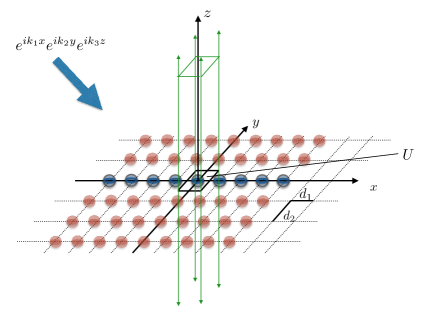
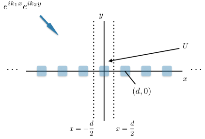
Figure 1: On the left is a periodic two-dimensional array of spherical scatterers lying in the $xy$-plane, with an incident plane wave at frequency $k=\sqrt{k_{1}^{2}+k_{2}^{2}+k_{3}^{2}}$ traveling in the direction $(k_{1},k_{2},k_{3})$. The unit cell is denoted by $U$. On the right is a periodic one-dimensional array of scatterers lying along the $x$-axis, with an incident plane wave at frequency $k=\sqrt{k_{1}^{2}+k_{2}^{2}}$ traveling in the direction $(k_{1},k_{2})$. The unit cell is again denoted by $U$.

Without entering into the details of integral equation methods or multiple scattering theory [5, 20, 24], we note that the Green’s function for the Helmholtz equation in free space is given by

$$G_{3D}(x,y,z)=\frac{e^{ikr}}{4\pi r}={\left(\frac{ik}{4\pi}\right)}h_{0}(kr),\quad G_{2D}(x,y,z)=\frac{H_{0}(kr)}{4i}\,,$$

in three and two dimensions, respectively, where $r=\sqrt{x^{2}+y^{2}+z^{2}}$ or $\sqrt{x^{2}+y^{2}}$ depending on the dimension, $h_{0}(x)$ denotes the spherical Hankel function of order zero, and $H_{0}(x)$ denotes the standard Hankel function of order zero. For quasiperiodic scattering, the Green’s function can be expressed formally as

$$G^{QP}_{3D}(x,y,z) =\frac{ik}{4\pi}\sum_{n=-\infty}^{\infty}\sum_{m=-\infty}^{\infty}h_{0}(k\sqrt{(x-nd_{1})^{2}+(y-md_{2})^{2}+z^{2}})e^{ink_{1}d_{1}}e^{imk_{2}d_{2}}\,,$$ (2)

$$G^{QP}_{2D}(x,y) =\frac{1}{4i}\sum_{n=-\infty}^{\infty}H_{0}(k\sqrt{(x-nd)^{2}+y^{2}})e^{ik_{1}nd}\,.$$ (3)

Note that both formulas (2) and (3) are simply infinite series of translated fundamental solutions.

By making use of standard addition theorems [20], it is straightforward and well-known that we can write

$$G^{QP}_{3D}(x,y,z)=\frac{ik}{4\pi}\left[h_{0}(kr)+\sum_{l=0}^{\infty}\sum_{j=-l}^{l}S_{l,j}Y_{l}^{-j}(\theta,\phi)j_{l}(kr)\right]\,,$$

where

$$S_{l,j} =S_{l,j}(d_{1},d_{2},k,k_{1},k_{2})$$

$$=\sum_{\begin{subarray}{c}n,m=-\infty\\ (n,m)\neq(0,0)\end{subarray}}^{\infty}h_{l}(k\sqrt{(nd_{1})^{2}+(md_{2})^{2}})Y_{l}^{j}\left(\frac{\pi}{2},\phi_{n}^{m}\right)e^{ink_{1}d_{1}}e^{imk_{2}d_{2}}\,.$$ (4)

Here, $h_{n}$ and $j_{n}$ denote the spherical Hankel and Bessel functions of order $n$ and $\phi_{n}^{m}$ is the angle subtended by the point $(nd_{1},md_{2})$ with respect to the $x$-axis. The function $Y_{l}^{j}$ denotes the spherical harmonic of degree $l$ and order $j$:

$$Y_{l}^{j}(\theta,\phi)=\sqrt{\frac{2l+1}{4\pi}}\sqrt{\frac{(l-|j|)!}{(l+|j|)!}}\,P_{l}^{|j|}(\cos\theta)e^{ij\phi}\,,$$ (5)

where the associated Legendre functions $P_{l}^{j}$ can be defined by the Rodrigues’ formula

$$P_{l}^{j}(x)=(-1)^{j}(1-x^{2})^{j/2}\frac{d^{j}}{dx^{j}}P_{l}(x),$$

with $P_{l}(x)$ the standard Legendre polynomial of degree $l$.

Similarly, in two dimensions, we have

$$G^{QP}_{2D}(x,y,z)=\frac{1}{4i}\left[H_{0}(kr)+\sum_{l=-\infty}^{\infty}S_{l}J_{l}(kr)e^{il\theta}\right]\,,$$

where $H_{n}$ and $J_{n}$ denote the usual Hankel and Bessel functions and

$$S_{l}=S_{l}(d,k,k_{1})=\sum_{n\in\mathbb{Z}\backslash\{0\}}H_{l}(|n|kd)(\operatorname{sgn}n)^{l}e^{ik_{1}nd}\,.$$ (6)

The sums appearing in (4) and (6) are referred to as lattice sums [11, 17, 18, 23]. If the expressions in (2), (3) (4) and (6) were well-defined, it would be straightforward to verify that $G^{QP}_{3D}$ and $G^{QP}_{2D}$ satisfy the desired quasiperiodicity conditions.

Unfortunately, three fundamental difficulties are encountered in the use of lattice sums: they are conditionally convergent, their “direct” numerical evaluation is extremely slow by naive methods, and they diverge for certain values of the wave parameters $k_{1},k_{2},k_{3}$ and lattice parameters $d_{1}$ and $d_{2}$ - giving rise to what are known as Wood’s anomalies [26]. The behavior of the scattered field is quite striking in the neighborhood of those parameter values, as discussed in [4, 11, 16] and in some detail below. In the two-dimensional case, it is straightforward to see from Fourier analysis that the scattered field (away from the obstacle) must take the form [11]

$$u^{scat}(x,y)=\sum_{n=-\infty}^{\infty}a_{n}e^{2\pi inx/d}e^{ik_{1}x}e^{i\beta_{n}y}\,,$$

for $y>0$ and

$$u^{scat}(x,y)=\sum_{n=-\infty}^{\infty}b_{n}e^{2\pi inx/d}e^{ik\cos\psi x}e^{-i\beta_{n}y}\,,$$

for $y<0$, where $\beta_{n}^{2}+\left(k_{1}+\frac{2\pi n}{d}\right)^{2}=k^{2}$ with the root taken as positive real or positive imaginary. Real values of $\beta_{n}$ correspond to propagating modes, while values of $\beta_{n}$ on the positive imaginary axis correspond to evanescent modes. Wood’s anomalies occur when $\beta_{n}=0$ and the scattered wave is propagating exactly along the array in the $x$-direction - a very special type of physical resonance. In three dimensions, the scattered field (away from the plane of obstacles) must take the form

$$u^{scat}(x,y,z)=\sum_{m,n\in\mathbb{Z}}a_{m,n}e^{2\pi inx/d_{1}}e^{ik_{1}x}e^{2\pi imy/d_{2}}e^{ik_{2}y}e^{i\beta_{n,m}z}\,,$$

for $z>0$ and

$$u^{scat}(x,y,z)=\sum_{m,n\in\mathbb{Z}}b_{m,n}e^{2\pi inx/d_{1}}e^{ik_{1}x}e^{2\pi imy/d_{2}}e^{ik_{2}y}e^{-i\beta_{n,m}z}\,,$$

for $z<0$, where

$$\beta_{n,m}^{2}+\left(k_{1}+\frac{2\pi n}{d_{1}}\right)^{2}+\left(k_{2}+\frac{2\pi m}{d_{2}}\right)^{2}=k^{2}.$$ (7)

Wood’s anomalies occur when $\beta_{n,m}=0$ and the scattered wave is propagating in some direction along the $xy$-plane [15, 22, 12].

The computation of lattice sums and the resonant behavior corresponding to Wood’s anomalies have been widely studied, from both a physical and a mathematical perspective (see, for example, [4, 10, 11, 12, 13, 16, 17, 18, 19, 22, 23, 27]). Oddly enough, in the numerical literature for evaluating lattice sums, the occurence of Wood’s anomalies is often ignored, despite the fact that the series can diverge and despite the potential loss of accuracy in computational results near such singularities.

In this paper, we focus on the rigorous analysis of one-dimensional lattice sums using a novel method based on quadrature, Euler-MacLaurin corrections to the trapezoidal rule, and steepest descent arguments. The reason for concentrating on the one-dimensional case is the remarkable work of McPhedran, Nicorovici, Botten, Grubits, Enoch and Nixon [8, 17], who showed that, once the one-dimensional lattice sums along the $x$-axis are obtained, highlighted in blue on the left-hand side of Fig. 1, the remaining contributions in higher dimensions can be computed semi-analytically using the Poisson summation formula. This technique, sometimes referred to as lattice reduction [13], is outlined briefly in section 2.

From a physical perspective, the correct choice of the conditionally convergent lattice sums corresponds to adding an infinitesimal amount of dissipation: that is, we replace the real wave number $k$ by $k+i\epsilon$ and then let $\epsilon\rightarrow 0^{+}$. For any fixed $\epsilon>0$, the relevant infinite series converges absolutely. Thus, instead of (6) and (4), we define the conditionally convergent lattice sums by

$$S_{l}=\lim_{\epsilon\rightarrow 0^{+}}\sum_{n\in\mathbb{Z}\backslash\{0\}}H_{l}(|n|(k+i\epsilon)d)(\operatorname{sgn}n)^{l}e^{ik_{1}nd}\,$$ (8)

and

$$S_{l,j}=\lim_{\epsilon\rightarrow 0^{+}}\sum_{\begin{subarray}{c}n,m=-\infty\\ (n,m)\neq(0,0)\end{subarray}}^{\infty}h_{l}((k+i\epsilon)\sqrt{(nd_{1})^{2}+(md_{2})^{2}})Y_{l}^{j}\left(\frac{\pi}{2},\phi_{n}^{m}\right)e^{ink_{1}d_{1}}e^{imk_{2}d_{2}}\,.$$ (9)

The existence of these limits will be established in our analysis, and the original physical interpretation does not play a role. We will show that the one-dimensional sums may be evaluated through techniques of complex analysis, combined with the Euler-Maclaurin formula with superalgebraic convergence. Our fast algorithm is derived in sections 3 and 6, and with proofs collected in sections 4 and 5. Section 7 presents some numerical experiments, and section 8 contains some concluding remarks.

2 Lattice Reduction

We illustrate the lattice reduction technique of [8, 17] for the case shown on the left-hand side of Fig. 1, with the added simplification that we assume the lattice to be square with unit cell of area one ($d_{1}=d_{2}=1$). For the prescribed wavenumber $k$, the Bloch phases are then given by $(e^{i\alpha},e^{i\beta})=(e^{ik_{1}},e^{ik_{2}})$. For the sake of brevity, we consider only the lattice sum $S_{0,0}$ from (4) which now takes the form:

$$S_{0,0} =\sum_{(n,m)\neq(0,0)}h_{0}(k\sqrt{n^{2}+m^{2}})e^{i\alpha n}e^{i\beta m}$$

$$=S_{0,0}^{+}+S^{grating}_{0,0}+S_{0,0}^{-}\,,$$ (10)

where

$$S_{0,0,}^{+}=\sum_{m>0}\sum_{n}h_{0}(k\sqrt{n^{2}+m^{2}})e^{i\alpha n}e^{i\beta m}\,,\quad S_{0,0}^{-}=\sum_{m<0}\sum_{n}h_{0}(k\sqrt{n^{2}+m^{2}})e^{i\alpha n}e^{i\beta m}\,,$$

and

$$S_{0,0}^{grating}=\sum_{n\neq 0}h_{0}(k|n|)e^{i\alpha n}\,.$$ (11)

Let us consider the sum $S^{+}_{0,0}$, which we write in the form

$$S^{+}_{0,0}=\sum_{m>0}\sum_{n\in\mathbb{Z}}h_{0}(k\sqrt{n^{2}+m^{2}})e^{i\alpha n}e^{i\beta m}\,=\ \sum_{m>0}e^{i\beta m}s_{m}\,,$$

where

$$s_{m}=\sum_{n\in\mathbb{Z}}h_{0}(k\sqrt{n^{2}+m^{2}})e^{i\alpha n}\,.$$

($S^{-}_{0,0}$ is treated in an analogous fashion.)

The important things to note about $s_{m}$ are (1) that it is the sum of the function $h_{0}(k\sqrt{x^{2}+m^{2}})e^{i\alpha x}$ sampled at the integers $n$, (2) that the function is smooth since $m>0$, and (3) that the spherical Hankel function $h_{0}$ has the spectral representation [5, 20, 24]

$$h_{0}(k\sqrt{x^{2}+y^{2}+z^{2}})=\frac{1}{2\pi ik}\int_{-\infty}^{\infty}\int_{-\infty}^{\infty}\frac{e^{-y\sqrt{s^{2}+t^{2}-k^{2}}}}{\sqrt{s^{2}+t^{2}-k^{2}}}e^{isx}e^{itz}\,ds\,dt\,,$$

for $y>0$. From this, letting $x=n$, $y=m$, and $z=0$, we have

$$s_{m}=\frac{1}{2\pi ik}\sum_{n\in\mathbb{Z}}\int_{-\infty}^{\infty}\int_{-\infty}^{\infty}\frac{e^{-m\sqrt{s^{2}+t^{2}-k^{2}}}}{\sqrt{s^{2}+t^{2}-k^{2}}}e^{in(s+\alpha)}\,ds\,dt\,.$$

We now apply the Poisson summation formula [17, 23], which we write informally as

$$\sum_{n}e^{inx}=2\pi\,\sum_{n}\delta(x+2\pi n).$$

This yields

$$s_{m}=\frac{1}{ik}\sum_{n\in\mathbb{Z}}\int_{-\infty}^{\infty}\frac{e^{-m\sqrt{t^{2}-k^{2}+(2\pi n-\alpha)^{2}}}}{\sqrt{t^{2}-k^{2}+(2\pi n-\alpha)^{2}}}\,dt.$$

From this, we have

$$S^{+}_{0,0}= \frac{1}{ik}\sum_{m>0}\sum_{n\in\mathbb{Z}}e^{i\beta m}\int_{-\infty}^{\infty}\frac{e^{-m\sqrt{t^{2}-k^{2}+(2\pi n-\alpha)^{2}}}}{\sqrt{t^{2}-k^{2}+(2\pi n-\alpha)^{2}}}\,dt$$

$$= \frac{1}{ik}\sum_{n\in\mathbb{Z}}\int_{-\infty}^{\infty}\frac{e^{i\beta-\sqrt{t^{2}-k^{2}+(2\pi n-\alpha)^{2}}}}{\sqrt{t^{2}-k^{2}+(2\pi n-\alpha)^{2}}}\,\frac{1}{1-e^{i\beta-\sqrt{t^{2}-k^{2}+(2\pi n-\alpha)^{2}}}}\,dt.$$

The last expression is obtained by summing a geometric series in the index $m$. Assuming that this formal manipulation makes sense, the resulting integral is rapidly converging in $t$ and the outer summation is rapidly converging in $n$. We omit further details, referring the reader to [8, 17]. Suffice it to say that, as a result of this observation, the principal obstacle in evaluating the lattice sum $S_{0,0}$ is that of computing the one-dimensional sum $S^{grating}_{0,0}$ in (11). This “punctured sum” cannot be evaluated through the Poisson summation formula directly, since the summand at $n=0$ is undefined (although Ewald type methods could be used to overcome this [11]).

The remainder of this paper is devoted to a new approach for the punctured sum, which results in a fast algorithm and may be of mathematical interest in its own right.

3 One-dimensional lattice sums and the Euler-
MacLaurin formula

To develop a unified framework that can handle one-dimensional sums such as $S^{grating}_{0,0}$ in (11) or $S_{l}$ in (6), let us now fix $k\in\mathbb{R}$, $d>0$ and suppose that $f(z)$ is a complex-analytic function such that, for some $\beta>0$, there exists a representation for the $p$th derivative of the form

$$f^{(p)}(z)=\frac{\Phi_{p}(z)}{z^{\beta}}e^{iz}\,,$$ (12)

where $\Phi_{p}(z)$ has an asymptotic series $\Phi_{p}(z)\sim\sum_{\mu=0}^{\infty}c_{p,\mu}z^{-\mu}$ valid for $|\textnormal{arg}\,z|<\pi/2+\delta$ and $|z|\rightarrow\infty$, for sufficiently small $\delta>0$. We also assume that $\Phi_{p}$ is bounded on the region $\left\{|z|>\delta^{\prime},\;|\textnormal{arg}\,z|<\pi/2+\delta\right\}$, for each $\delta^{\prime}>0$. The Bessel functions $h_{n}$ and $H_{n}$ are well-known to satisfy such estimates [1].

For $\epsilon>0$ and $\alpha\in\mathbb{R}$, we define the function

$${F}_{\alpha}^{\epsilon}(z)=f\left((k+i\epsilon)z\right)e^{i\alpha z}\,.$$ (13)

We shall denote by $F_{\alpha}$ the corresponding expression with $\epsilon=0$. For reasons that will become apparent later, we shall assume that $\left\{(k\pm\alpha)d/2\pi\right\}\cap\mathbb{Z}=\varnothing$. We now consider absolutely convergent sums of the general form:

$${S}^{\epsilon}(\alpha)=\sum_{n>0}{F}_{\alpha}^{\epsilon}(nd)\,.$$ (14)

Clearly, for $\ell\in\mathbb{Z}$, sums of the form

$$\sum_{n\in\mathbb{Z}\setminus\{0\}}f((k+i\epsilon)|nd|)(\textnormal{sgn}\,n)^{l}e^{i\alpha nd}={S}^{\epsilon}(\alpha)+(-1)^{\ell}{S}^{\epsilon}(-\alpha),$$

so we shall concern ourselves primarily with ${S}^{\epsilon}(\alpha)$. This framework covers the cases of physical interest in quasiperiodic scattering.

Our approach will require the use of an infinitely differentiable filter function, which we introduce here.

Definition 3.1

Let $\psi\in C^{\infty}([0,1])$ be a decreasing function such that, for some $r$ with $0<r<\frac{1}{4}$, $\psi|_{[0,2r]}=1$ and $\psi|_{[1-2r,1]}=0$. For $b,c\in\mathbb{N}$, we denote the scaled filter function $\psi_{b,c}(x)$ by

$$\psi_{b,c}(x)=\begin{cases}1,&x<b\,,\\ \psi\left[\frac{1}{c}(x-b)\right],&b\leq x\leq b+c\,,\\ 0,&b+c<x\,.\end{cases}$$ (15)

See Fig. 2. Note that the parameter $r$ determines both how flat the scaled filter function $\psi_{b,c}(x)$ is at the points $x=b$ and $x=b+c$, and how steep the transition is from $1$ to $0$.

From the properties of $\psi_{b,c}$, we may write

$${S}^{\epsilon}(\alpha)=\sum_{n=1}^{b-1}{F}_{\alpha}^{\epsilon}(nd)+\sum_{n=b}^{b+c}{F}_{\alpha}^{\epsilon}(nd)\psi_{b,c}(n)+\sum_{n=b}^{\infty}{F}_{\alpha}^{\epsilon}(nd)(1-\psi_{b,c}(n))\,.$$

Note that the third term corresponds to the trapezoidal approximation for the integral

$$\int_{b}^{\infty}{F}_{\alpha}(xd)(1-\psi_{b,c}(x))\,dx.$$

We now show that this integral can be evaluated by contour deformation and that the difference between the integral and the desired sum can be computed with high precision using Euler-MacLaurin corrections.

Lemma 3.1

Let $\phi\in(-\pi/2,\pi/2)$, such that $\tan\phi=(k+\alpha)/\epsilon$. Then

$$\int_{b}^{\infty}{F}_{\alpha}^{\epsilon}(xd)\,dx=\,\frac{1}{d}\int_{0}^{\infty}{F}_{\alpha}^{\epsilon}(bd+\zeta\tau)\,\zeta\,d\tau$$

where $\zeta=e^{i\phi}=\frac{\epsilon+i(k+\alpha)}{\sqrt{\epsilon^{2}+(k+\alpha)^{2}}}$.

Let $C_{0}$, $C_{\phi}$ denote the outward rays in the complex plane with $\arg z=0$ and $\arg z=\phi$. We begin by writing

$$\int_{b}^{\infty}{F}_{\alpha}^{\epsilon}(xd)\,dx=\frac{1}{d}\int_{0}^{\infty}{F}_{\alpha}^{\epsilon}(bd+t)\,dt=\frac{1}{d}\int_{C_{0}}{F}_{\alpha}^{\epsilon}(bd+z)\,dz$$

Now let $C_{0}(R)=[0,R]$ and let $C_{\phi}(R)=[0,R\zeta]$. Let $B(R)$ denote the circular arc from $R$ to $R\zeta$, let $I=[0,\phi]$ if $\phi>0$, and let $I=[\phi,0]$ if $\phi<0$. It is straightforward to verify that

$$\left|\int_{B(R)}{F}_{\alpha}^{\epsilon}(bd+z)\,dz\right|= \left|\int_{I}{F}_{\alpha}^{\epsilon}(bd+Re^{i\phi^{\prime}})Rie^{i\phi^{\prime}}d\phi^{\prime}\right|\,\leq\frac{C}{(|k|bd)^{\beta}}\cdot Re^{-\epsilon R\cos\phi}\,,$$

which goes to zero as $R\rightarrow\infty$. This justifies the contour deformation from $C_{0}$ to $C_{\phi}$:

$$\int_{b}^{\infty}{F}_{\alpha}^{\epsilon}(xd)\,dx=\,\frac{1}{d}\int_{C_{\phi}}{F}_{\alpha}^{\epsilon}(bd+z)\,dz=\,\frac{1}{d}\int_{0}^{\infty}{F}_{\alpha}^{\epsilon}\left(bd+\zeta\tau\right)\zeta\,d\tau\,.$$

$\square$

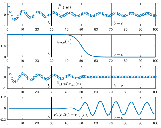
Figure 2: Lattice sums and the Euler-MacLaurin formula: The top row shows the discrete values of ${F}_{\alpha}(nd)$ whose sum corresponds to ${S}(\alpha)$. The second row depicts an infinitely differentiable filter function $\psi_{b,c}(x)$, which equals $1$ for $x\leq b$ and $0$ for $x>b+c$. The third row is a plot of the discrete values ${F}_{\alpha}(nd)\psi_{b,c}(n)$ and the bottom row is a plot of ${F}_{\alpha}(xd)(1-\psi_{b,c}(x))$. Our method exploits the relation between the desired lattice sum and the improper integral $\int_{n=b}^{\infty}{F}_{\alpha}(xd)(1-\psi_{b,c}(x))\,dx,$ which involves Euler-MacLaurin corrections at the endpoints.

Theorem 3.1

Let $\psi_{b,c}$ be a scaled filter function (Definition 3.1.) Then, for any fixed integer $s\geq 2$, we have

$${S}^{\epsilon}(\alpha)= \sum_{n=1}^{b-1}{F}_{\alpha}^{\epsilon}(nd)+\sum_{n=b}^{b+c}{F}_{\alpha}^{\epsilon}(nd)\psi_{b,c}(n)-\int_{b}^{b+c}{F}_{\alpha}^{\epsilon}(xd)\psi_{b,c}(x)\,dx$$ (16)

$$+\frac{1}{d}\int_{0}^{\infty}{F}_{\alpha}^{\epsilon}\left(bd+\frac{\epsilon+i(k+\alpha)}{\sqrt{\epsilon^{2}+(k+\alpha)^{2}}}\tau\right)\frac{\epsilon+i(k+\alpha)}{\sqrt{\epsilon^{2}+(k+\alpha)^{2}}}\,d\tau+R_{s,b,c}^{\epsilon}(\alpha)\,,$$

where

$$R_{s,b,c}^{\epsilon}(\alpha)=\frac{(-1)^{s-1}}{s!}\int_{b}^{\infty}B_{s}(x-[x])\left[\left.\frac{d^{s}}{dt^{s}}\left({F}_{\alpha}^{\epsilon}(td)(1-\psi_{b,c}(t))\right)\right|_{t=x}\right]\,dx\,,$$ (17)

and $B_{s}(x)$ denotes the Bernoulli polynomial of order $s$.

We have

$${S}^{\epsilon}(\alpha)=\sum_{n>0}{F}_{\alpha}^{\epsilon}(nd)\\ =\,\sum_{n>0}{F}_{\alpha}^{\epsilon}(nd)\psi_{b,c}(n)+\sum_{n>0}{F}_{\alpha}^{\epsilon}(nd)(1-\psi_{b,c}(n))\,.$$ (18)

Since $\psi_{b,c}(n)=1$, for $n\leq b$, and $\psi_{b,c}(n)=0$, for $n>b+c$, we have

$${S}^{\epsilon}(\alpha)=\sum_{n=1}^{b-1}{F}_{\alpha}^{\epsilon}(nd)+\sum_{n=b}^{b+c}{F}_{\alpha}^{\epsilon}(nd)\psi_{b,c}(n)+\sum_{n=b+1}^{\infty}{F}_{\alpha}^{\epsilon}(nd)(1-\psi_{b,c}(n))\,.$$

We now employ the Euler-Maclaurin formula (see [2], p. 619, Theorem D.2.1) to find that, for $s\in\mathbb{N}\backslash\{0\}$, $N>b$,

$$\sum_{n=b+1}^{N}{F}_{\alpha}^{\epsilon}(nd)(1-\psi_{b,c}(n))= \int_{b}^{N}{F}_{\alpha}^{\epsilon}(xd)(1-\psi_{b,c}(x))\,dx$$

$$+\sum_{\gamma=1}^{s}\frac{(-1)^{\gamma}B_{\gamma}}{\gamma!}\left.\frac{d^{\gamma-1}}{dx^{\gamma-1}}\left({F}_{\alpha}^{\epsilon}(xd)(1-\psi_{b,c}(x))\right)\right|_{x=N}$$

$$-\sum_{\gamma=1}^{s}\frac{(-1)^{\gamma}B_{\gamma}}{\gamma!}\left.\frac{d^{\gamma-1}}{dx^{\gamma-1}}\left({F}_{\alpha}^{\epsilon}(xd)(1-\psi_{b,c}(x))\right)\right|_{x=b}$$

$$+\frac{(-1)^{s-1}}{s!}\int_{b}^{N}B_{s}(x-[x])\left[\left.\frac{d^{s}}{dt^{s}}\left({F}_{\alpha}^{\epsilon}(td)(1-\psi_{b,c}(t))\right)\right|_{t=x}\right]\,dx\,,$$

where the $B_{s}(x)$ are the Bernoulli polynomials, and the $B_{\gamma}$ are Bernoulli numbers. Observe that $(1-\psi_{b,c}(x))$ is identically zero in a neighborhood of $x=b$ and that the boundary term at $x=b$ vanishes outright. Moreover, ${F}_{\alpha}^{\epsilon}(xd)$ and all its derivatives tend to zero exponentially as $x\rightarrow\infty$. Thus, only the two integral terms on the right hand side of the Euler-Maclaurin formula are preserved in the limit $N\rightarrow\infty$.

Thus,

$$\sum_{n=b+1}^{\infty}{F}_{\alpha}^{\epsilon}(nd)(1-\psi_{b,c}(n))= \int_{b}^{\infty}{F}_{\alpha}^{\epsilon}(xd)(1-\psi_{b,c}(x))\,dx+R_{s,b,c}^{\epsilon}(\alpha)$$

$$= \int_{b}^{\infty}{F}_{\alpha}^{\epsilon}(xd)\,dx-\int_{b}^{b+c}{F}_{\alpha}^{\epsilon}(xd)\psi_{b,c}(x)\,dx+R_{s,b,c}^{\epsilon}(\alpha)\,,$$

and

$${S}^{\epsilon}(\alpha)=\sum_{n=1}^{b-1}{F}_{\alpha}^{\epsilon}(nd)+\sum_{n=b}^{b+c}{F}_{\alpha}^{\epsilon}(nd)\psi_{b,c}(n)-\int_{b}^{b+c}{F}_{\alpha}^{\epsilon}(xd)\psi_{b,c}(x)\,dx+\int_{b}^{\infty}{F}_{\alpha}^{\epsilon}(xd)\,dx+R_{s,b,c}^{\epsilon}(\alpha)\,.$$

The desired result now follows from Lemma 3.1. $\square$

Before turning to the algorithm itself, we will require two more results, whose proofs are deferred to the next sections.

Lemma 3.2

The term $R_{s,b,c}^{\epsilon}(\alpha)$ from eq. (17) satisfies the estimate

$$\lim_{c\rightarrow\infty}\underset{\epsilon\rightarrow 0^{+}}{\overline{\lim}}\left|R_{s,b,c}^{\epsilon}(\alpha)\right|=\mathcal{O}(c^{-N-\beta})$$

for any fixed $N$.

Lemma 3.3

Recall that ${F}_{\alpha}^{\epsilon}(z)=f((k+i\epsilon)z)e^{i\alpha z}$ and for $p\in\mathbb{N}\cup\left\{0\right\}$ and $q\in\mathbb{Z}$ let

$$G_{\alpha,p,q}^{\epsilon}(x)=-\int_{x}^{\infty}f^{(p)}((k+i\epsilon)td)e^{i\alpha td}e^{2\pi iqt}\,dt\,.$$ (19)

Then $G_{\alpha,p,q}(x)\equiv\lim_{\epsilon\rightarrow 0^{+}}G_{\alpha,p,q}^{\epsilon}(x)$ exists (see formula (24)) and

$$\lim_{c\rightarrow\infty}\limsup_{\epsilon\rightarrow 0^{+}} \left|\sum_{n=b}^{b+c}{F}_{\alpha}^{\epsilon}(nd)\psi_{b,c}(n)-\int_{b}^{b+c}{F}_{\alpha}^{\epsilon}(xd)\psi_{b,c}(x)dx-\mathcal{A}\right|=0$$ (20)

where

$$\mathcal{A}={F}_{\alpha}(bd)-\sum_{\gamma=1}^{s}\frac{(-1)^{\gamma}B_{\gamma}}{\gamma!}\left.\frac{d^{\gamma-1}}{dx^{\gamma-1}}\left({F}_{\alpha}(xd)\right)\right|_{x=b}$$ (21)

$$-\frac{(-1)^{s-1}}{s!}A_{s}\sum_{j_{1}=0}^{s}\binom{s}{j_{1}}d^{s}k^{s-j_{1}}(i\alpha)^{j_{1}}\left[\sum_{q\in\mathbb{Z}\backslash\left\{0\right\}}q^{-s}G_{\alpha,s-j_{1},q}(b)\right]\,,$$

where $A_{s}=-s!/(2\pi i)^{s}$ (see [1], 23.1.16).

4 Proof of Lemma 3.2

For Lemma 3.2, we need to estimate the remainder $R_{s,b,c}^{\epsilon}(\alpha)$, defined via (17). This is precisely the error incurred by using the Euler-Maclaurin formula.

We begin by using the generalized product rule to expand the derivatives in (17):

$$R_{s,b,c}^{\epsilon}(\alpha)= \frac{(-1)^{s-1}}{s!}\int_{b}^{\infty}B_{s}(x-[x])\left[\left.\frac{d^{s}}{dt^{s}}\left({F}_{\alpha}^{\epsilon}(td)(1-\psi_{b,c}(t))\right)\right|_{t=x}\right]\,dx$$

$$= \frac{(-1)^{s-1}}{s!}\sum_{j=0}^{s}\sum_{j_{1}=0}^{s-j}\binom{s}{j}\binom{s-j}{j_{1}}d^{s-j}(k+i\epsilon)^{s-j-j_{1}}(i\alpha)^{j_{1}}$$

$$\times\int_{b}^{\infty}B_{s}(x-[x])(\delta_{j,0}-\psi_{b,c}^{(j)}(x))f^{(s-j-j_{1})}((k+i\epsilon)xd)e^{i\alpha xd}\,dx\,.$$

We see that it suffices to verify the smallness of finitely many terms of the following form:

$$\mathcal{R}_{\alpha,b,c,p,j}^{\epsilon}=\int_{b}^{\infty}B_{s}(x-[x])(\delta_{j,0}-\psi_{b,c}^{(j)}(x))f^{(p)}((k+i\epsilon)xd)e^{i\alpha xd}\,dx\,.$$ (22)

The functions $B_{s}(x-[x])$ are Bernoulli polynomials, and for $s\geq 2$ we have the absolutely convergent Fourier expansion:

$$B_{s}(x-[x])=A_{s}\cdot\sum_{q\in\mathbb{Z}\backslash\{0\}}q^{-s}e^{2\pi iqx}\,,$$

with $A_{s}=(-1)s!/(2\pi i)^{s}$ (see [1], 23.1.16). We shall assume henceforth that $s\geq 2$ to guarantee convergence; then by Fubini’s theorem, we have

$$\mathcal{R}_{\alpha,b,c,p,j}^{\epsilon}=A_{s}\sum_{q\in\mathbb{Z}\backslash\{0\}}q^{-s}\int_{b}^{\infty}(\delta_{j,0}-\psi_{b,c}^{(j)}(x))f^{(p)}((k+i\epsilon)xd)e^{i\alpha xd}e^{2\pi iqx}\,dx\,.$$

Let us define (for $x>0$)

$$G_{\alpha,p,q}^{\epsilon}(x)=-\int_{x}^{\infty}f^{(p)}((k+i\epsilon)td)e^{i\alpha td}e^{2\pi iqt}\,dt\,.$$ (23)

Integrating by parts, we have

$$\mathcal{R}_{\alpha,b,c,p,j}^{\epsilon}= A_{s}\sum_{q\in\mathbb{Z}\backslash\{0\}}q^{-s}\int_{b}^{\infty}\psi_{b,c}^{(j+1)}(x)G_{\alpha,p,q}^{\epsilon}(x)\,dx$$

$$= A_{s}\sum_{q\in\mathbb{Z}\backslash\{0\}}q^{-s}\int_{b}^{b+c}\psi_{b,c}^{(j+1)}(x)G_{\alpha,p,q}^{\epsilon}(x)\,dx$$

$$= A_{s}c^{-j}\sum_{q\in\mathbb{Z}\backslash\{0\}}q^{-s}\int_{0}^{1}\psi^{(j+1)}(x)G_{\alpha,p,q}^{\epsilon}(b+cx)\,dx\,.$$

Let $\lambda_{q}=(\alpha+k)d+2\pi q$, and let $\psi\in(-\pi/2,\pi/2)$ such that $\tan\psi=\lambda_{q}(d\epsilon)^{-1}$. Since we assumed that $(k\pm\alpha)d/2\pi\notin\mathbb{Z}$, we have that $\lambda_{q}\neq 0$ for any $q\in\mathbb{Z}$; indeed, it holds that $\inf_{q\in\mathbb{Z}}|\lambda_{q}|>0$. Let $C_{0}$, $C_{\psi}$ be contours in the $z$-plane along the outward rays $\arg z=0$ and $\arg z=\psi$. We have

$$G_{\alpha,p,q}^{\epsilon}(x)= -\int_{x}^{\infty}f^{(p)}((k+i\epsilon)td)e^{i\alpha td}e^{2\pi iqt}\,dt$$

$$= -\int_{C_{0}}\frac{\Phi_{p}((k+i\epsilon)(x+z)d)}{[(k+i\epsilon)(x+z)d]^{\beta}}e^{i(\lambda_{q}+id\epsilon)(x+z)}\,dz$$

$$= -e^{i(\lambda_{q}+id\epsilon)x}\int_{C_{0}}\frac{\Phi_{p}((k+i\epsilon)(x+z)d)}{[(k+i\epsilon)(x+z)d]^{\beta}}e^{i(\lambda_{q}+id\epsilon)z}\,dz$$

We now deform the contour $C_{0}$ into $C_{\psi}$, which will be justified momentarily.

$$G_{\alpha,p,q}^{\epsilon}(x)= -e^{i(\lambda_{q}+id\epsilon)x}\int_{C_{\psi}}\frac{\Phi_{p}((k+i\epsilon)(x+z)d)}{[(k+i\epsilon)(x+z)d]^{\beta}}e^{i(\lambda_{q}+id\epsilon)z}\,dz$$

$$= -e^{i(\lambda_{q}+id\epsilon)x}\int_{0}^{\infty}\frac{\Phi_{p}((k+i\epsilon)(x+e^{i\psi}\tau)d)}{[(k+i\epsilon)(x+e^{i\psi}\tau)d]^{\beta}}e^{i(\lambda_{q}+id\epsilon)(\cos\psi+i\sin\psi)\tau}e^{i\psi}\,d\tau$$

$$= -e^{i(\lambda_{q}+id\epsilon)x}\int_{0}^{\infty}\frac{\Phi_{p}((k+i\epsilon)(x+e^{i\psi}\tau)d)}{[(k+i\epsilon)(x+e^{i\psi}\tau)d]^{\beta}}e^{-\tau\sqrt{\lambda_{q}^{2}+d^{2}\epsilon^{2}}}e^{i\psi}\,d\tau\,.$$

This implies that $G_{\alpha,p,q}^{\epsilon}(x)$ is bounded on $[1,\infty)$ uniformly as $\epsilon\rightarrow 0^{+}$, $|q|\rightarrow\infty$, moreover, by the dominated convergence theorem (with $\eta=\operatorname{sgn}\lambda_{q}$),

$$\lim_{\epsilon\rightarrow 0^{+}}G_{\alpha,p,q}^{\epsilon}(x)=-e^{i\lambda_{q}x}i\eta\int_{0}^{\infty}\frac{\Phi_{p}((x+i\eta\tau)kd)}{[(x+i\eta\tau)kd]^{\beta}}e^{-|\lambda_{q}|\tau}\,d\tau\,.$$ (24)

The contour deformation in the above calculation, which takes place at some fixed $\epsilon>0$, is justified by the following estimate, where $B(R)$ and $I$ are defined as on the proof of Lemma 3.1.

$$\ \left|\int_{B(R)}\frac{\Phi_{p}((k+i\epsilon)(x+z)d)}{[(k+i\epsilon)(x+z)d]^{\beta}}e^{i(\lambda_{q}+id\epsilon)z}dz\right|\hskip 93.95122pt$$

$$= \ \left|\int_{I}\frac{\Phi_{p}((k+i\epsilon)(x+Re^{i\psi^{\prime}})d)}{[(k+i\epsilon)(x+Re^{i\psi^{\prime}})d]^{\beta}}e^{iR(\lambda_{q}+id\epsilon)(\cos\psi^{\prime}+i\sin\psi^{\prime})}Rie^{i\psi^{\prime}}d\psi^{\prime}\right|$$

$$\leq \ CR(|k|xd)^{-\beta}\int_{I}e^{-|\lambda_{q}|R\sin|\psi^{\prime}|}e^{-\epsilon dR\cos\psi^{\prime}}d\psi^{\prime}$$

$$\leq \ C(|k|xd)^{-\beta}\cdot Re^{-\epsilon dR\cos\psi}\longrightarrow 0\textnormal{ as }R\rightarrow\infty\,.$$

Let us define $G_{\alpha,p,q}(x)=\lim_{\epsilon\rightarrow 0^{+}}G_{\alpha,p,q}^{\epsilon}(x)$; we desire an asymptotic approximation to this function as $x\rightarrow\infty$. Recall that we have an asymptotic approximation $\Phi_{p}(z)\sim\sum_{\mu=0}^{\infty}c_{p,\mu}z^{-\mu}$, $|z|\rightarrow\infty$. Thus, for any fixed $N\geq 1$, we have

$$G_{\alpha,p,q}(x)= -e^{i\lambda_{q}x}i\eta\int_{0}^{\infty}\frac{\Phi_{p}((x+i\eta\tau)kd)}{[(x+i\eta\tau)kd]^{\beta}}e^{-|\lambda_{q}|\tau}\,d\tau$$

$$= -e^{i\lambda_{q}x}i\eta\left(\sum_{\mu=0}^{N}\frac{c_{p,\mu}}{(kd)^{\mu+\beta}}\int_{0}^{\infty}\frac{e^{-|\lambda_{q}|\tau}}{(x+i\eta\tau)^{\mu+\beta}}\,d\tau+\mathcal{O}(x^{-N-\beta})\right)\,,$$

Now we integrate by parts iteratively, finitely many times, until the error term is $\mathcal{O}(x^{-N-\beta})$.

$$G_{\alpha,p,q}(x)= -e^{i\lambda_{q}x}i\eta\left(\sum_{\mu=0}^{N}\sum_{\nu=0}^{N-\mu}\frac{c_{p,\mu}(i\eta)^{\nu}\prod_{0\leq i_{1}<\nu}(-\mu-\beta-i_{1})}{(kd)^{\mu+\beta}|\lambda_{q}|^{\nu+1}}x^{-(\mu+\nu)-\beta}+\mathcal{O}(x^{-N-\beta})\right)$$

$$= -e^{i\lambda_{q}x}i\eta\left(\sum_{\rho=0}^{N}\sum_{\mu=0}^{\rho}\frac{c_{p,\mu}(i\eta)^{\rho-\mu}\prod_{0\leq i_{1}<(\rho-\mu)}(-\mu-\beta-i_{1})}{(kd)^{\mu+\beta}|\lambda_{q}|^{\rho-\mu+1}}x^{-\rho-\beta}+\mathcal{O}(x^{-N-\beta})\right)$$

$$= -e^{i\lambda_{q}x}i\eta\left(\sum_{\rho=0}^{N-1}\left[\sum_{\mu=0}^{\rho}\frac{c_{p,\mu}(i\eta)^{\rho-\mu}\prod_{0\leq i_{1}<(\rho-\mu)}(-\mu-\beta-i_{1})}{(kd)^{\mu+\beta}|\lambda_{q}|^{\rho-\mu+1}}\right]x^{-\rho-\beta}+\mathcal{O}(x^{-N-\beta})\right)\,.$$

In particular, we find that $G_{\alpha,p,q}(x)\sim e^{i\lambda_{q}x}\sum_{\rho=0}^{\infty}G_{\rho,p,q}x^{-\rho-\beta}$; moreover, since $k$ and $d$ are fixed, we have an estimate $|G_{\rho,p,q}|\leq C_{\rho,p}\cdot(1+|\lambda_{q}|^{-\rho-1})$. Since $\left\{(k\pm\alpha)d/2\pi\right\}\cap\mathbb{Z}=\varnothing$, we have that $\inf_{q}|\lambda_{q}|>0$, so for fixed $\rho$, $G_{\rho,p,q}$ is uniformly bounded in $q$. Additionally, the error estimate $\mathcal{O}(x^{-N-\beta})$ is uniform in $q$, in that both the constant and the domain of validity are uniform in $q$, if $N$ is held constant. (This relies on $\inf_{q}|\lambda_{q}|>0$.)

Recall that

$$\mathcal{R}_{\alpha,b,c,p,j}^{\epsilon}=A_{s}c^{-j}\sum_{q\in\mathbb{Z}\backslash\{0\}}q^{-s}\int_{0}^{1}\psi^{(j+1)}(x)G_{\alpha,p,q}^{\epsilon}(b+cx)\,dx\,.$$

Since $G_{\alpha,p,q}^{\epsilon}(x)$ is uniformly bounded in the simultaneous limit $\epsilon\rightarrow 0^{+}$, $|q|\rightarrow\infty$, we may use the dominated convergence theorem to commute the limit $\epsilon\rightarrow 0^{+}$ with the integral, as well as the sum over $q$:

$$\lim_{\epsilon\rightarrow 0^{+}}\mathcal{R}_{\alpha,b,c,p,j}^{\epsilon}=A_{s}c^{-j}\sum_{q\in\mathbb{Z}\backslash\{0\}}q^{-s}\int_{0}^{1}\psi^{(j+1)}(x)G_{\alpha,p,q}(b+cx)\,dx\,.$$

By using $G_{\alpha,p,q}(x)=e^{i\lambda_{q}x}\sum_{\rho=0}^{N-1}G_{\rho,p,q}x^{-\rho-\beta}+\mathcal{O}(x^{-N-\beta})$ (the error estimate being uniform in $q$), and the fact that $\forall j\geq 0$, $\psi^{(j+1)}(x)$ is identically zero on $[0,2r]$, we have (in the limit $c\rightarrow\infty$)

$$\lim_{\epsilon\rightarrow 0^{+}}\mathcal{R}_{\alpha,b,c,p,j}^{\epsilon}$$

$$= A_{s}c^{-j}\sum_{\rho=0}^{N-1}\sum_{q\in\mathbb{Z}\backslash\{0\}}\frac{G_{\rho,p,q}e^{i\lambda_{q}b}}{q^{s}}\int_{r}^{1-r}\psi^{(j+1)}(x)\frac{e^{i\lambda_{q}cx}}{(b+cx)^{\rho+\beta}}\,dx+\mathcal{O}(c^{-j-N-\beta})$$

$$= A_{s}c^{-j}\sum_{\rho=0}^{N-1}\sum_{q\in\mathbb{Z}\backslash\{0\}}\frac{G_{\rho,p,q}e^{i\lambda_{q}b}}{c^{\rho+\beta}q^{s}}\int_{r}^{1-r}\frac{\psi^{(j+1)}(x)}{x^{\rho+\beta}}e^{i\lambda_{q}cx}\left(1+\frac{b}{cx}\right)^{-\rho-\beta}\,dx+\mathcal{O}(c^{-j-N-\beta})$$

Since $c$ is large and $x\geq r$, we may expand $(1+b/cx)^{-\rho-\beta}$ in powers of $(b/cx)$.

$$\lim_{\epsilon\rightarrow 0^{+}}\mathcal{R}_{\alpha,b,c,p,j}^{\epsilon}$$

$$= A_{s}\sum_{\rho=0}^{N-1}\sum_{\omega=0}^{N-\rho-1}\left[(-1)^{\omega}\frac{\prod_{i_{1}=0}^{\omega-1}(\rho+i_{1}+\beta)}{\omega!b^{-\omega}c^{j+\rho+\omega+\beta}}\sum_{q\in\mathbb{Z}\backslash\{0\}}\frac{G_{\rho,p,q}e^{i\lambda_{q}b}}{q^{s}}\int_{r}^{1-r}\frac{\psi^{(j+1)}(x)}{x^{\rho+\omega+\beta}}e^{i\lambda_{q}cx}\,dx\right]$$

$$+\mathcal{O}(c^{-j-N-\beta})\,.$$

Note that the integral on the right hand side depends on $c$ only through $e^{i\lambda_{q}cx}$, and $\psi^{(j+1)}(x)/x^{\rho+\omega+\beta}$ is smooth and compactly supported on $[r,1-r]$. Thus, the integral decays faster than any power of $c^{-1}$ as $c\rightarrow\infty$, and such decay is uniform in $q$.

Thus, as $c\rightarrow\infty$, for any fixed $N$, we have

$$\lim_{\epsilon\rightarrow 0^{+}}\mathcal{R}_{\alpha,b,c,p,j}^{\epsilon}=\mathcal{O}(c^{-j-N-\beta}),$$

yielding the desired result. $\square$

5 Proof of Lemma 3.3

For Lemma 3.3 we employ the Euler-Maclaurin formula yet again.

$$\sum_{n=b}^{b+c}{F}_{\alpha}^{\epsilon}(nd)\psi_{b,c}(n)-\int_{b}^{b+c}{F}_{\alpha}^{\epsilon}(xd)\psi_{b,c}(x)\,dx$$

$$= {F}_{\alpha}^{\epsilon}(bd)+\sum_{\gamma=1}^{s}\frac{(-1)^{\gamma}B_{\gamma}}{\gamma!}\left[\left.\frac{d^{\gamma-1}}{dx^{\gamma-1}}\left({F}_{\alpha}^{\epsilon}(xd)\psi_{b,c}(x)\right)\right|_{x=b+c}-\left.\frac{d^{\gamma-1}}{dx^{\gamma-1}}\left({F}_{\alpha}^{\epsilon}(xd)\psi_{b,c}(x)\right)\right|_{x=b}\right]$$

$$+\frac{(-1)^{s-1}}{s!}\int_{b}^{b+c}B_{s}(x-[x])\left[\left.\frac{d^{s}}{dt^{s}}\left({F}_{\alpha}^{\epsilon}(td)\psi_{b,c}(t)\right)\right|_{t=x}\right]\,dx\,.$$

Since $\psi_{b,c}(x)$ is identically zero in a neighborhood of $b+c$ and identically one in a neighborhood of $b$, this reduces to

$$\sum_{n=b}^{b+c}{F}_{\alpha}^{\epsilon}(nd)\psi_{b,c}(n)-\int_{b}^{b+c}{F}_{\alpha}^{\epsilon}(xd)\psi_{b,c}(x)\,dx$$

$$= {F}_{\alpha}^{\epsilon}(bd)-\sum_{\gamma=1}^{s}\frac{(-1)^{\gamma}B_{\gamma}}{\gamma!}\left.\frac{d^{\gamma-1}}{dx^{\gamma-1}}\left({F}_{\alpha}^{\epsilon}(xd)\right)\right|_{x=b}$$

$$+\frac{(-1)^{s-1}}{s!}\int_{b}^{b+c}B_{s}(x-[x])\left[\left.\frac{d^{s}}{dt^{s}}\left({F}_{\alpha}^{\epsilon}(td)\psi_{b,c}(t)\right)\right|_{t=x}\right]\,dx\,.$$

We expand the derivatives as before and define

$$\mathcal{E}_{\alpha,b,c,p,j}^{\epsilon}=\int_{b}^{b+c}B_{s}(x-[x])\psi_{b,c}^{(j)}(x)f^{(p)}((k+i\epsilon)xd)e^{i\alpha xd}\,dx\,,$$ (25)

$$E_{\alpha,b,c}^{\epsilon}= \frac{(-1)^{s-1}}{s!}\sum_{j=0}^{s}\sum_{j_{1}=0}^{s-j}\binom{s}{j}\binom{s-j}{j_{1}}d^{s-j}(k+i\epsilon)^{s-j-j_{1}}(i\alpha)^{j_{1}}\mathcal{E}_{\alpha,b,c,s-j-j_{1},j}^{\epsilon}\,.$$ (26)

Then

$$\sum_{n=b}^{b+c}{F}_{\alpha}^{\epsilon}(nd)\psi_{b,c}(n)-\int_{b}^{b+c}{F}_{\alpha}^{\epsilon}(xd)\psi_{b,c}(x)dx$$ (27)

$$= {F}_{\alpha}^{\epsilon}(bd)-\sum_{\gamma=1}^{s}\frac{(-1)^{\gamma}B_{\gamma}}{\gamma!}\left.\frac{d^{\gamma-1}}{dx^{\gamma-1}}\left({F}_{\alpha}^{\epsilon}(xd)\right)\right|_{x=b}+E_{\alpha,b,c}^{\epsilon}\,.$$

The limit of each term as $\epsilon\rightarrow 0^{+}$ exists (trivially for the first two terms, by the dominated convergence theorem for the third):

$$\lim_{\epsilon\rightarrow 0^{+}}\left[\sum_{n=b}^{b+c}{F}_{\alpha}^{\epsilon}(nd)\psi_{b,c}(n)-\int_{b}^{b+c}{F}_{\alpha}^{\epsilon}(xd)\psi_{b,c}(x)dx\right]$$

$$= {F}_{\alpha}(bd)-\sum_{\gamma=1}^{s}\frac{(-1)^{\gamma}B_{\gamma}}{\gamma!}\left.\frac{d^{\gamma-1}}{dx^{\gamma-1}}\left({F}_{\alpha}(xd)\right)\right|_{x=b}+\lim_{\epsilon\rightarrow 0^{+}}E_{\alpha,b,c}^{\epsilon}\,.$$

Notice that the first two terms are fully independent of $c$; to complete the argument, it suffices to show that $\lim_{c\rightarrow\infty}\lim_{\epsilon\rightarrow 0^{+}}\mathcal{E}_{\alpha,b,c,p,j}^{\epsilon}$ exists (we do not claim a limit of zero). Moreover, the $c\rightarrow\infty$ convergence behavior of the desired limit is fully determined by the $c\rightarrow\infty$ convergence behavior of $\lim_{\epsilon\rightarrow 0^{+}}\mathcal{E}_{\alpha,b,c,p,j}^{\epsilon}$.

As before, we replace $B_{s}(x-[x])$ by its absolutely convergent Fourier expansion ($s\geq 2$) and use Fubini’s theorem:

$$\mathcal{E}_{\alpha,b,c,p,j}^{\epsilon}= \int_{b}^{b+c}B_{s}(x-[x])\psi_{b,c}^{(j)}(x)f^{(p)}((k+i\epsilon)xd)e^{i\alpha xd}dx$$ (28)

$$= A_{s}\sum_{q\in\mathbb{Z}\backslash\{0\}}q^{-s}\int_{b}^{b+c}\psi_{b,c}^{(j)}(x)f^{(p)}((k+i\epsilon)xd)e^{i\alpha xd}e^{2\pi iqx}dx$$

$$= -A_{s}\left[\delta_{j,0}\sum_{q\in\mathbb{Z}\backslash\{0\}}q^{-s}G_{\alpha,p,q}^{\epsilon}(b)+\sum_{q\in\mathbb{Z}\backslash\{0\}}q^{-s}\int_{b}^{b+c}\psi_{b,c}^{(j+1)}(x)G_{\alpha,p,q}^{\epsilon}(x)dx\right]$$

$$= -A_{s}\delta_{j,0}\sum_{q\in\mathbb{Z}\backslash\{0\}}q^{-s}G_{\alpha,p,q}^{\epsilon}(b)-\mathcal{R}_{\alpha,b,c,p,j}^{\epsilon}\,.$$

Due to the uniform boundedness of $G_{\alpha,p,q}^{\epsilon}(x)$ on $[1,\infty)$ in the simultaneous limit $\epsilon\rightarrow 0^{+}$, $|q|\rightarrow\infty$, we may commute the $\epsilon\rightarrow 0^{+}$ limit with the sum in the first term:

$$\limsup_{\epsilon\rightarrow 0^{+}}\left|\mathcal{E}_{\alpha,b,c,p,j}^{\epsilon}+A_{s}\delta_{j,0}\sum_{q\in\mathbb{Z}\backslash\{0\}}q^{-s}G_{\alpha,p,q}(b)\right|=\limsup_{\epsilon\rightarrow 0^{+}}\left|\mathcal{R}_{\alpha,b,c,p,j}^{\epsilon}\right|\,.$$ (29)

The right-hand side is $\mathcal{O}(c^{-j-N-1/2})$ as $c\rightarrow\infty$, for any $N$, as has already been established.

$\square$

6 Informal description of the algorithm

Using equations (16) and Lemma 3.3, we can conclude the existence of $\lim_{\epsilon\rightarrow 0^{+}}{S}^{\epsilon}(\alpha)$ and obtain an explicit formula for this quantity (for a fixed $s\geq 2$):

$$\lim_{\epsilon\rightarrow 0^{+}}{S}^{\epsilon}(\alpha)= \sum_{n=1}^{b}{F}_{\alpha}(nd)-\sum_{\gamma=1}^{s}\frac{(-1)^{\gamma}B_{\gamma}}{\gamma!}\left.\frac{d^{\gamma-1}}{dx^{\gamma-1}}\left({F}_{\alpha}(xd)\right)\right|_{x=b}$$ (30)

$$+\frac{1}{d}\int_{0}^{\infty}{F}_{\alpha}\left(bd+i\tau\textnormal{sgn}(k+\alpha)\right)i\textnormal{sgn}(k+\alpha)d\tau$$

$$-\frac{(-1)^{s-1}}{s!}A_{s}\sum_{j_{1}=0}^{s}\binom{s}{j_{1}}d^{s}k^{s-j_{1}}(i\alpha)^{j_{1}}\left[\sum_{q\in\mathbb{Z}\backslash\left\{0\right\}}q^{-s}G_{\alpha,s-j_{1},q}(b)\right]\,.$$

While this formula is mathematically interesting, it does not provide a convenient algorithm due to the presence of terms depending on $G_{\alpha,p,q}(b)$. Instead, our algorithm approximates this limit by computing the first four terms of the formula (16) at $\epsilon=0$, for larger and larger values of $c$. Specifically, the expression is evaluated for increasing $c$ at fixed $b$ until convergence is obtained with the desired number of digits. This procedure is formally justified due to Lemma 3.2 and Lemma 3.3.

It is, perhaps, of interest to note that the conditional convergence of the lattice sums is discussed in the literature (see, for example [11]), but not typically studied in terms of an explicit limit with vanishing dissipation. An exception is [7].

6.1 Wood anomalies

As noted in the introduction, when $(k\pm\alpha)d=2\pi n$, where $n\in\mathbb{Z}$, the lattice sums considered in this paper may actually diverge. Such singularities are known as Wood’s anomalies and correspond to a kind of physical resonance in the underlying system. Using (30) and (24), we expect to see $|{S}(\alpha)|\lesssim|\delta k|^{-\frac{1}{2}}$ for sums involving $H_{\ell}$ and $|{S}(\alpha)|\lesssim\log\frac{1}{|\delta k|}$ for sums involving $h_{\ell}$ as $|\delta k|\rightarrow 0$. Here, $|\delta k|$ is the distance (in the wavenumber variable $k$) to the closest Wood anomaly. Two dimensional Wood anomalies (see (7)), are more complicated to characterize and will be considered at a later date.

7 Numerical Validation

Our fast summation algorithm for one-dimensional lattice sums, as previously indicated, is based upon the formula (16),

$${S}^{\epsilon}(\alpha)= \sum_{n>0}{F}_{\alpha}^{\epsilon}(nd)=\sum_{n>0}f((k+i\epsilon)nd)e^{i\alpha nd}$$

$$= \sum_{n=1}^{b-1}{F}_{\alpha}^{\epsilon}(nd)+\sum_{n=b}^{b+c}{F}_{\alpha}^{\epsilon}(nd)\psi_{b,c}(n)-\int_{b}^{b+c}{F}_{\alpha}^{\epsilon}(xd)\psi_{b,c}(x)\,dx$$

$$+\frac{1}{d}\int_{0}^{\infty}{F}_{\alpha}^{\epsilon}\left(bd+\frac{\epsilon+i(k+\alpha)}{\sqrt{\epsilon^{2}+(k+\alpha)^{2}}}\tau\right)\frac{\epsilon+i(k+\alpha)}{\sqrt{\epsilon^{2}+(k+\alpha)^{2}}}\,d\tau+R_{s,b,c}^{\epsilon}(\alpha)\,.$$

Using Lemma 3.2 and Lemma 3.3 which have been proven in the preceding sections, if $c$ is sufficiently large then

$$\lim_{\epsilon\rightarrow 0^{+}}{S}^{\epsilon}(\alpha)\approx \sum_{n=1}^{b-1}{F}_{\alpha}(nd)+\sum_{n=b}^{b+c}{F}_{\alpha}(nd)\psi_{b,c}(n)-\int_{b}^{b+c}{F}_{\alpha}(xd)\psi_{b,c}(x)\,dx$$ (31)

$$+\frac{1}{d}\int_{0}^{\infty}{F}_{\alpha}\left(bd+i\tau\textnormal{sgn}\left(k+\alpha\right)\right)i\,\textnormal{sgn}\left(k+\alpha\right)\,d\tau\,.$$

Moreover, for any fixed cutoff function $\psi$ as in the statement of Theorem 3.1, the error associated with this approximation vanishes more quickly than any power of $c$, as $c\rightarrow\infty$.

The fast algorithm proceeds as follows: First, we fix (once and for all) a smooth cut-off function $\psi$ as in the statement of Theorem 3.1. We also fix a positive integer value for the parameter $b$, which does not play an essential role in the analysis. Second, we evaluate the right-hand side of (31) for integer values of $c$, doubling $c$ at each iteration until convergence is obtained.

To test the speed and accuracy of our algorithm, we consider the cases where $f$ is the Hankel function of the first kind $H_{\ell}^{(1)}$ or the spherical Hankel function of the first kind $h_{\ell}^{(1)}$. With a Fortran implementation on a 1.3GHz Intel Core M processor, we found that the first 120 lattice sums $S_{l}$ in (6) were computed in 1.2 milliseconds with $7$ digits of accuracy for $k=1$, with a unit cell of length $d=1$ and $\alpha=0.4$. For $k=10$, 1.5 milliseconds were required and for $k=100$, 300 lattice sums were computed in 2 milliseconds. For validation, the sums ${S}^{\epsilon}(\alpha)$ were computed directly for $\epsilon>0$, and the limit $\epsilon\rightarrow 0^{+}$ was determined numerically using fourth-order Richardson extrapolation starting at $\epsilon=10^{-3}$, with an estimated accuracy of twelve digits.

In Fig. 3, we scan a range of frequencies $k$ with the phase $\alpha$ set to either $0$ or $0.4$. The blowup of $S_{0}$, defined by (6) is clearly visible. To investigate the behavior of our numerical method near Wood anomalies, we set parameters to $d=1$, $\alpha=\frac{\pi}{4}$, and $k=\frac{7\pi}{4}+\eta$, where $0<\eta\leq 1$, and consider the lattice sums $S_{l}$ involving $H_{\ell}$ and $h_{\ell}$, respectively. In Fig. 4, we plot $S_{l}$ and $S^{grating}_{l,0}$, defined as the one-dimensional grating sum component of (4), for $l=0,1,2,3$. In the first case, there is a clear power-law singularity with the correct exponent. In the latter case, involving $h_{\ell}$, the blowup is only logarithmic and harder to fit precisely.

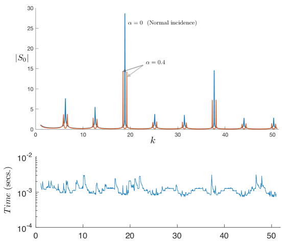
Figure 3: (Top) The periodic blowup of the lattice sums $S_{0}(\alpha)$, defined by (6) as a function of frequency $k$, with $\alpha$ set to either $0$ or $0.4$ and $d=1$. (Bottom) Time required for lattice sums with $\alpha=0.4$ at eack $k$.

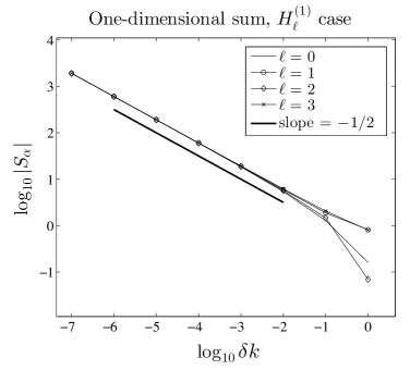
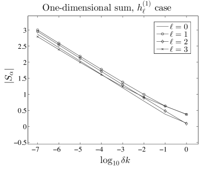
Figure 4: (l) Power-law blow-up of $S_{l}(\alpha)$ near a Wood’s anomaly when $f=H^{(1)}_{\ell}$ with parameters $d=1$, $\alpha=\frac{\pi}{4}$, $k=\frac{7\pi}{4}+\delta k$. (r) Blow-up of the lattice sums $S^{grating}_{l,0}(\alpha)$ near a Wood’s anomaly when $f=h^{(1)}_{\ell}$, with the same parameters. Note that on the left, the $y$-axis is on a logarithmic scale, while on the right, it is on a linear scale.

8 Conclusions

We have described a general approach for the numerical evaluation of one-dimensonal lattice sums which play an important role in diffraction and wave propagation problems in both two and three dimensions. Indeed, it is often possible to efficiently reduce higher-dimensional sums to their one-dimensional counterparts as discussed in section 2. Our algorithm achieves super-algebraic convergence rates and is able to evaluate lattice sums accurately and efficiently. Moreover, our estimates supply an interesting analytic interpretation of Wood’s anomalies - physical resonances that occur when $(k\pm\alpha)d=2\pi n$ for integer $n$ - which cause the lattice sums to diverge [12, 11]. In particular, the formulas (24) and (30) allow us to directly estimate the type of blow-up one should expect to see.

We believe that higher dimensional Wood anomalies can be analyzed by coupling our method with lattice reduction techniques, and we will report on such work at a later date. Finally, it is worth noting that lattice sums can be avoided altogether. Quasiperiodic boundary conditions can be imposed, for example, using layer potentials [3, 4, 9], fundamental solutions [6], or spherical harmonics [14] to enforce the conditions explicitly. Which approach is more efficient will depend, we suspect, on the ambient dimension, the frequency, and on the aspect ratio of the unit cell. Both this question and a comparison with other fast algorithms, such as those discussed in [10, 11, 12, 13, 16, 17, 18, 19, 23, 27] remain to be explored.

References

[1]
M. Abramowitz and I. A. Stegun.
Handbook of Mathematical Functions.
Dover, 1972.
[2]
G. E. Andrews, R. Askey, and R. Roy.
Special Functions.
Cambridge University Press, 1999.
[3]
A. Barnett and L. Greengard.
A new integral representation for quasi-periodic fields and its
application to two-dimensional band structure calculations.
Journal of Computational Physics, 229:6898–6914, 2010.
[4]
A. Barnett and L. Greengard.
A new integral representation for quasi-periodic scattering problems
in two dimensions.
BIT Numer. Math., 51(1):67–90, 2011.
[5]
W. C. Chew, editor.
Waves and Fields in Inhomogeneous Media.
IEEE Press, New York, 1995.
[6]
Min Hyung Cho and Alex H. Barnett.
Robust fast direct integral equation solver for quasi-periodic
scattering problems with a large number of layers.
Optics Express, 23:1775–1799, 2015.
[7]
Andrew Dienstfrey, Fengbo Hang, and Jingfang Huang.
Lattice sums and the two-dimensional, periodic Green’s function for
the Helmholtz equation.
Proceedings of the Royal Society A: Mathematical, Physical and
Engineering Sciences, 457:67–85, 2001.
[8]
S. Enoch, R. C. McPhedran, N. A. Nicorovici, L. C. Botten, and J. N. Nixon.
Sums of spherical waves for lattices, layers, and lines.
J. Math. Phys., 42:5859–5870, 2001.
[9]
Adrianna Gillman and Alex H. Barnett.
A fast direct solver for quasi-periodic scattering problems.
Journal of Computational Physics, 248:309–322, 2013.
[10]
H. Kurkcu and F. Reitich.
Stable and efficient evaluation of periodized green’s functions for
the Helmholtz equation at high frequencies.
Journal of Computational Physics, 228:75–95, 2009.
[11]
C. M. Linton.
Lattice sums for the Helmholtz equation.
SIAM Rev., 52(4):630–674, 2010.
[12]
C. M. Linton and I. Thompson.
Resonant effects in scattering by periodic arrays.
Wave Motion, 44(3):165–175, 2007.
[13]
C. M. Linton and I. Thompson.
One- and two-dimensional lattice sums for the three-dimensional
Helmholtz equation.
J. Comp. Phys., 228(6):1815, 2009.
[14]
Yuxiang Liu and Alex H. Barnett.
Efficient numerical solution of acoustic scattering from
doubly-periodic arrays of axisymmetric objects, 2015.
accepted, J. Comput. Phys.; arxiv:1506.05083.
[15]
Yuxiang Liu and Alex H. Barnett.
Efficient numerical solution of acoustic scattering from
doubly-periodic arrays of axisymmetric objects.
Journal of Computational Physics, 324:226 – 245, 2016.
[16]
Daniel Maystre.
Theory of Wood’s Anomalies.
In S. Enoch and N. Bonod, editors, Plasmonics, chapter 2.
Springer, Berlin, 2012.
[17]
R. C. McPhedran, N. A. Nicorovici, L. C. Botten, and K. A. Grubits.
Lattice sums for gratings and arrays.
J. Math. Phys., 41(11):7808–7816, 2000.
[19]
A. Moroz.
Quasi-periodic Green’s functions of the
Helmholtz and Laplace equations.
J. Phys. A: Math. Gen., 39(36):11247, 2006.
[20]
P. Morse and H. Feshbach, editors.
Methods of Theoretical Physics.
McGraw-Hill, New York, 1953.
[21]
R. Petit, editor.
Electronmgnetic Theory of Gratings.
Springer, Heidelberg, 1980.
[22]
Stephen P. Shipman.
Resonant scattering by open periodic waveguides.
In Matthias Ehrhardt, editor, Wave Propagation in Periodic
Media: Progress in Computational Physics, vol. 1, pages 7 – 50. Bentham
Books, Berlin, 2010.
[23]
V. Twersky.
Elementary function representations of Schlomilch series.
Arch. Ration. Mech. Anal., 8(1):323–332, 1961.
[24]
H. C. van de Hulst, editor.
Light Scattering by Small Particles.
Dover, New York, 1981.
[25]
Calvin H. Wilcox, editor.
Scattering Theory for Diffraction Gratings.
Springer, New York, 2013.
[26]
R. W. Wood.
On a remarkable case of uneven distribution of light in a diffraction
grating spectrum.
Philos. Mag., 4:396–408, 1902.
[27]
K. Yasumoto and K. Yoshitomi.
Efficient calculation of lattice sums for free-space periodic
Green’s function.
IEEE Trans. Antennas Propag., 47(6):1050, 1999.