Extraction of the $\pi^{+}\pi^{-}$ Subsystem in Diffractively Produced $\pi^{-}\pi^{+}\pi^{-}$ at Compass

Abstract

The Compass experiment at CERN has collected a large data sample of 50 million diffractively produced $\pi^{-}\pi^{+}\pi^{-}$ events using a $190\,$GeV$/c$ negatively charged hadron beam. The partial-wave analysis (PWA) of these high-precision data reveals previously unseen details. The PWA, which is currently limited by systematic uncertainties, is based on an isobar model, where multi-particle decays are described as subsequent two-body decays and where a prior-knowledge parametrization for the intermediate two-pion resonances has to be assumed – usually a Breit-Wigner amplitude – thus increasing systematic uncertainties, due to the concrete choice of the parametrization. We present a novel method, which allows to extract isobar amplitudes directly from the data in a less biased way. The focus lies on the scalar $\pi^{+}\pi^{-}$ subsystem, where a previous analysis found a signal for a new axial-vector state $a_{1}(1420)$ decaying into $f_{0}(980)\pi$.

1 Introduction

Compass is a two-stage multi-purpose spectrometer, located at CERN’s Prévessin site, which employs secondary hadron or tertiary muon beams from the Super Proton Synchrotron. Its large acceptance over a wide kinematic range allows Compass to study a broad physics program including, amongst others, light-meson spectroscopy, which is the focus here.

The particular channel of interest is $\pi^{-}p\to\pi^{-}\pi^{+}\pi^{-}p$, for which Compass collected a data set consisting of approximately $50$ million events.

2 Analysis method

2.1 The Isobar Model

To analyze the process $\pi^{-}p\to X^{-}p\to\pi^{-}\pi^{+}\pi^{-}p$ we use the isobar model, which assumes that the appearing intermediate $3\pi$ state $X^{-}$ does not decay directly into $\pi^{-}\pi^{+}\pi^{-}$, but undergoes subsequent two-particle decays until it ends up in the final state: $X^{-}\to\xi^{0}\pi^{-}\to\pi^{-}\pi^{+}\pi^{-}$. The intermediate two-pion state $\xi^{0}$ is called the isobar.

2.2 Conventional PWA

The conventional PWA expands the complex decay amplitude, which describes the measured intensity distribution $\mathcal{I}$, into partial waves [1]:

$$\mathcal{I}(\vec{\tau};m_{3\pi},t^{\prime})=\left|\sum_{\mathrm{waves}}\mathcal{T}_{\mathrm{wave}}(m_{3\pi},t^{\prime})\Psi_{\mathrm{wave}}(\vec{\tau};m_{3\pi})\right|^{2}.$$ (1)

The production amplitudes $\mathcal{T}_{\mathrm{wave}}$ depend on the invariant mass $m_{3\pi}$ of the $\pi^{-}\pi^{+}\pi^{-}$ system and on the reduced squared four-momentum transfer $t^{\prime}$. They are fitted to the data in bins of their kinematic variables using an extended maximum likelihood fit.

For constant $m_{3\pi}$ and $t^{\prime}$, the decay amplitudes $\Psi_{\mathrm{wave}}$ depend on $5$ kinematic variables, that define the $3\pi$ kinematics and are represented by $\vec{\tau}$, while the angular part alone is given by $\vec{\Theta}$. The decay amplitudes are known functions, which have to be put into the analysis model beforehand. They consist of a mass-dependent part $\Delta_{\xi}(m_{\pi^{+}\pi^{-}})$ which depends on the mass of the $\pi^{+}\pi^{-}$ subsystem, and an angular part $\mathcal{K}(\vec{\Theta})$:

$$\Psi_{\mathrm{wave}}(\vec{\tau};m_{3\pi})=\Delta_{\xi}(m_{\pi^{+}\pi^{-}};m_{3\pi})\mathcal{K}(\vec{\Theta};m_{3\pi})+(\mathrm{Bose\ symm.}).$$ (2)

The angular-momentum quantum numbers appearing in a partial wave completely determine the function $\mathcal{K}(\vec{\Theta})$.

The complex function $\Delta_{\xi}(m_{\pi^{+}\pi^{-}};m_{3\pi})$ describes the complex amplitude of the corresponding isobar $\xi$ and usually has to be known without any free parameters. In the simplest cases, single Breit-Wigner amplitudes are used. Since no unique parametrizations for these amplitudes are given by theory and different models are available, the choice of a particular parametrization introduces a model bias.

A conventional PWA of this type, which was performed on the data-set collected by the Compass spectrometer, uses a set of $88$ waves [1] .

2.3 Freed-isobar PWA

In order to circumvent this problem we introduce a novel method, which was inspired by Ref. [2]. This method allows us to extract isobar amplitudes in bins of $m_{\pi^{+}\pi^{-}}$ directly from the data. To this end, the fixed parametrizations are replaced by sets of piece-wise constant functions:

$$\Pi_{\mathrm{bin}}(m_{\pi^{+}\pi^{-}})=\left\{\begin{array}[]{l}1\mathrm{\ if\ }m_{\pi^{+}\pi^{-}}\mathrm{\ lies\ in\ the\ corresponding\ mass\ bin,`}\\ 0\mathrm{\ otherwise.}\end{array}\right.$$ (3)

These binned functions replace the fixed isobar amplitudes:

$$\Delta_{\xi}(m_{\pi^{+}\pi^{-}})\to\sum_{\mathrm{bins}}\Pi_{\mathrm{bin}}(m_{\pi^{+}\pi^{-}}).$$ (4)

The set of bins covers the whole kinematically allowed $m_{\pi^{+}\pi^{-}}$ mass range. With this replacement, equation (1) reads:

$$\mathcal{I}(m_{\pi^{+}\pi^{-}},\vec{\Theta};m_{3\pi},t^{\prime})=\left|\sum_{\mathrm{waves}}\sum_{\mathrm{bins}}\mathcal{T}_{\mathrm{wave}}(m_{\pi^{+}\pi^{-}}^{\mathrm{bin}};m_{3\pi},t^{\prime})\left[\Pi_{\mathrm{bin}}(m_{\pi^{+}\pi^{-}})\mathcal{K}_{\mathrm{wave}}(\vec{\Theta})\right]+(\mathrm{Bose\ symm.})\right|^{2}.$$ (5)

The piece-wise constant isobar amplitudes effectively behave like independent partial waves and their corresponding production amplitudes now also encode information about th $m_{\pi^{+}\pi^{-}}$ dependence of the isobar amplitudes. Therefore, the same fit procedure as in the conventional approach can be used. We call this new approach freed-isobar PWA.

A freed-isobar wave is named after the folloing scheme:

$$J^{PC}M^{\varepsilon}[\pi\pi]_{J^{PC}_{\xi}}\pi L,$$ (6)

where $J^{PC}$ are the spin and eigenvalues und parity and generalized charge conjugation of the $3\pi$ system, while $M^{\varepsilon}$ are its spin projection and reflectivity. The term $[\pi\pi]$ denotes a freed-isobar wave with spin and eigenvalues und parity and charge conjugation of $J^{PC}_{\xi}$. Finally, $L$ is the orbital angular momentum between the isobar and the bachelor $\pi$.

3 First Application

The analysis presented in the following employs $3$ freed-isobar waves: $0^{-+}0^{+}[\pi\pi]_{0^{++}}\pi S$, $1^{++}0^{+}$ $[\pi\pi]_{0^{++}}\pi P$ and $2^{-+}0^{+}[\pi\pi]_{0^{++}}\pi D$. Due to quantum numbers of the $\pi^{+}\pi^{-}$ subsystem, these waves describe seven waves in the conventional scheme. Therefore, the final model consists of $81$ fixed and $3$ freed-isobar waves.

3.1 $0^{-+}0^{+}[\pi\pi]_{0^{++}}\pi\,S$ Wave

The $0^{-+}0^{+}[\pi\pi]_{0^{++}}\pi\,S$ wave is able to describe all three isobars that are used in the conventional PWA: the $f_{0}(500)$, the $f_{0}(980)$, and the $f_{0}(1500)$. Fig. 1 shows the two-dimensional intensity distribution
$\left|\mathcal{T}_{\text{wave}}(m_{3\pi},m_{\pi^{+}\pi^{-}})\right|^{2}$ for this wave for two bins in $t^{\prime}$.

The most striking feature is a peak corresponding to the decay $\pi(1800)\to f_{0}(980)\pi$. A smaller peak corresponding to $\pi(1800)\to f_{0}(1500)\,\pi^{-}$ is also visible. Broad structures appear at low $2\pi$ and $3\pi$ masses and low $t^{\prime}$, which are probably of mostly non-resonant origin.

Fig. 2 and Fig. 3 show the intensity distributions and Argand diagrams as a function of $m_{\pi^{+}\pi^{-}}$ in narrow $m_{3\pi}$ bins around the $\pi(1800)$ resonance. Peaks and phase motions corresponding to the $f_{0}(980)$ and the $f_{0}(1500)$ are visible. They are modulated by the intensity distribution and phase motion of the decay of $\pi(1800)$.

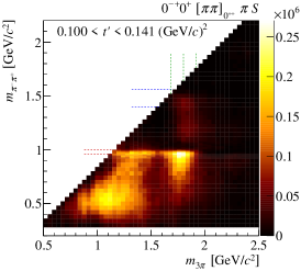
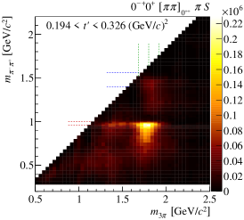
Figure 1: Intensity distribution of the $0^{-+}0^{+}[\pi\pi]_{0^{++}}\pi\,S$ wave as a function of $m_{3\pi}$ and $m_{\pi^{+}\pi^{-}}$ for two regions of $t^{\prime}$ [1].

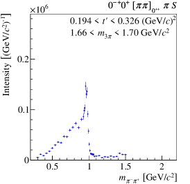
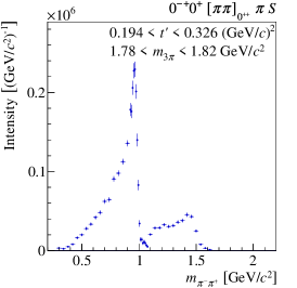
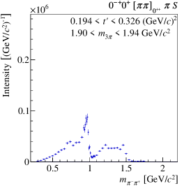
Figure 2: $0^{-+}0^{+}[\pi\pi]_{0^{++}}\pi S$ intensity distributions for three bins of $m_{3\pi}$, below, on, and above the $\pi(1800)$ resonance [1].

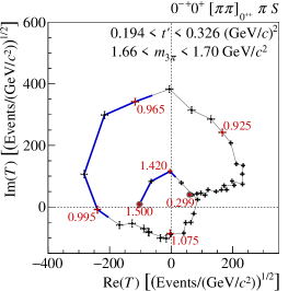
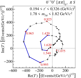
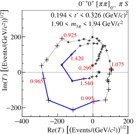
Figure 3: Argand diagrams of the $0^{-+}0^{+}[\pi\pi]_{0^{++}}\pi S$ amplitude for three bins of $m_{3\pi}$ below, on, and above the $\pi(1800)$ resonance. The $m_{\pi^{+}\pi^{-}}$ regions corresponding to the $f_{0}(980)$ and the $f_{0}(1500)$ are highlighted in blue [1].

3.2 $1^{++}0^{+}[\pi\pi]_{0^{++}}\pi\,P$ Wave

The freed $1^{++}0^{+}[\pi\pi]_{0^{++}}\pi\,P$ wave is able to describe two waves of the conventional PWA, since the $1^{++}0^{+}$ $f_{0}(1500)\pi P$ wave was not included in the conventional analysis. The two-dimensional intensity distribution is shown in Fig. 4 for two $t^{\prime}$ bins. It features a dominant broad structure at low $2\pi$ and $3\pi$ masses, which moves with $t^{\prime}$, indicating a predominantly non-resonant origin. In addition, a narrow peak at $m_{3\pi}\approx 1.4\,\mathrm{GeV}/c^{2}$ and a $m_{\pi^{+}\pi^{-}}\approx 0.98\,\mathrm{GeV}/c^{2}$ is visible. It corresponds to the recently discovered $a_{1}(1420)$ [3]. The observation of this peak in tha freed-isobar analysis proves that the $a_{1}(1420)$ signal is not an artifact of the parametrization of the scalar isobars in the conventional analysis [3].

Fig. 5 shows the $2\pi$ intensity distributions below, on, and above the $a_{1}(1420)$, which exhibits a strong correlation with the $f_{0}(980)$ peak. A comparison of the $f_{0}(980)$ mass region from the freed-isobar fit is in good agreement with the intensity of the $1^{++}0^{+}f_{0}(980)\pi P$ wave from the conventional PWA (See Fig. 6).

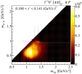
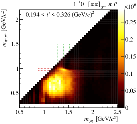
Figure 4: Intensity distribution of the $1^{++}0^{+}[\pi\pi]_{0^{++}}\pi\,P$ wave as a function of $m_{3\pi}$ and $m_{\pi^{+}\pi^{-}}$ for two regions of $t^{\prime}$ [1].

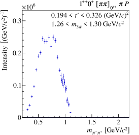
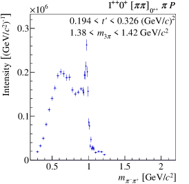
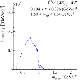
Figure 5: $1^{++}0^{+}[\pi\pi]_{0^{++}}\pi P$ intensity distributions for three bins of $m_{3\pi}$ around the $a_{1}(1420)$ resonance [1].

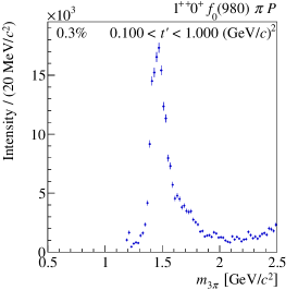
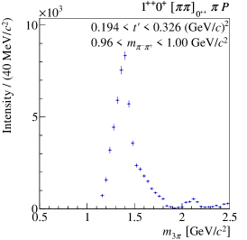
Figure 6: $1^{++}0^{+}f_{0}(980)\pi P$ intensity from the conventional PWA (left) and intensity sum over the $m_{\pi^{+}\pi^{-}}$ bins in the $f_{0}(980)$ region of the $1^{++}0^{+}[\pi\pi]_{0^{++}}\pi P$ wave from the freed-isobar analysis (right) [1].

4 Conclusions

We have introduced a novel PWA method for the process $\pi^{-}p\to\pi^{-}\pi^{+}\pi^{-}p$ using binned amplitudes to describe the $\pi^{+}\pi^{-}$ subsystems. This not only removes the model bias introduced by formerly fixed amplitudes used for the appearing isobars in the conventional PWA, but also allows us to study the $2\pi$ subsystems and their dependence on the $3\pi$ source system.

The large data set collected by the Compass spectrometer enables us to apply this novel method. In a first analysis, we free the $0^{++}$ isobar prametrizations for three waves with different $J^{PC}$ of the $3\pi$ parent system, namely $0^{-+}$, $1^{++}$, and $2^{-+}$. The analysis reproduces most of the expected structures, in particular a peak for the decay $a_{1}(1420)\to f_{0}(980)\pi$, which confirms the new signal observed with the conventional analysis not to be an artifact of the $f_{0}(980)$ parametrization.

In addition to resonances, broad structures are observed, that typically change their shape with $t^{\prime}$. They probably originate from non-resonant processes or from cross-talk with waves, that still employ fixed isobar amplitudes.

We are currently studying the latter effect by increasing the number of freed isobars. At the moment, we aim for a set of $11$ freed waves that would describe $75\%$ of the total intensity. In these fits, we encounter several ambiguities in the fit and are currently working on techniques to resolve them.

References

- [1] C. Adolph et al. [COMPASS Collaboration], arXiv:1509.00992 [hep-ex].
- [2] E. M. Aitala et al. [E791 Collaboration], Phys. Rev. D 73 (2006) 032004 [Phys. Rev. D 74 (2006) 059901] doi:10.1103/PhysRevD.73.032004, 10.1103/PhysRevD.74.059901 [hep-ex/0507099].
- [3] C. Adolph et al. [COMPASS Collaboration], Phys. Rev. Lett. 115 (2015), 082001