Stochastic epidemic dynamics on extremely heterogeneous networks

Abstract

Networks of contacts capable of spreading infectious diseases are often observed to be highly heterogeneous, with the majority of individuals having fewer contacts than the mean, and a significant minority having relatively very many contacts. We derive a two-dimensional diffusion model for the full temporal behavior of the stochastic susceptible-infectious-recovered (SIR) model on such a network, by making use of a time-scale separation in the deterministic limit of the dynamics. This low-dimensional process is an accurate approximation to the full model in the limit of large populations, even for cases when the time-scale separation is not too pronounced, provided the maximum degree is not of the order of the population size.

I Introduction

Mathematical models are used throughout infectious disease epidemiology to understand the dynamical processes that shape patterns of disease Rock et al. (2014); Heesterbeek et al. (2015). While early models did not include complex population structure, modeling approaches now frequently let the epidemic spread take place on a network, which enables greater realism than a model in which all individuals mix homogeneously. It does, however, pose many technical problems for model analysis, particularly the question of how heterogeneity in the number of links each individual participates in—their degree—influences the epidemic Danon et al. (2011); Pastor-Satorras et al. (2015); Pellis et al. (2015).

Similarly, even though some of the earliest mathematical models of infectious diseases were stochastic, accounting for the chance nature of transmission of infection Bailey (1957), much of the applied modeling that followed was deterministic and based on non-linear differential equations Anderson and May (1991). More recent applied work has, however, recognized the importance of using stochastic epidemic models King et al. (2015) and also of the development of associated methodology Britton et al. (2015).

The difficulty in mathematically analyzing models that include both stochastic elements and network structure can be a reason for not including these factors, but we prefer to include them, and subsequently to systematically reduce the complexity of the resulting model. This is the approach we adopt in this paper; the reduction process being made possible because of the existence of a separation of time-scales: many variables “decaying” away rapidly, leaving a few slow variables, which govern the medium- to long-term dynamics.

Compartmental models of epidemics typically assume that the majority of the population starts susceptible to infection, with a small number infectious, who then spread infection to others before recovering. A key distinction is between susceptible-infectious-susceptible (SIS) dynamics in which recovery returns an individual to the susceptible compartment and susceptible-infectious-recovered (SIR) dynamics in which recovery removes an individual from a further role in the next epidemic Pastor-Satorras et al. (2015), with the former being used to model, e.g., sexually transmitted infections other than HIV and the latter, e.g., pandemic influenza Anderson and May (1991); Keeling and Rohani (2007); Heesterbeek et al. (2015).

In the theoretical analysis of epidemic models, a crucial quantity corresponds to the basic reproductive ratio $R_{0}$—verbally described as the expected number of secondary cases infected per primary case early in the epidemic Diekmann et al. (1990). Depending on the value of $R_{0}$, either $\mathcal{O}(N)$ individuals will experience infection in a population of size $N$—the model is then said to be supercritical—or $\mathcal{O}(1)$ individuals will experience infection in a population of size $N$—the model is then subcritical—thus defining an epidemic threshold.

In reality, the contact network on which the disease spreads will often change over the course of the epidemic; while approaches exist in which the dynamics of both the disease and the network are considered Miller et al. (2012), it is more common to consider two limiting cases. The first of these is a static approach (also called ‘quenched’) in which the network is assumed to evolve much more slowly than the disease and which is typically approached analytically through the use of pair approximation and related techniques Miller et al. (2012); Eames and Keeling (2002). The second is a dynamic limit (also called ‘annealed’ or ‘discrete heterogeneous’) in which the network is assumed to evolve much more quickly than the epidemic, and can be described by an effective network characterized by its degree distribution, in which all individuals sharing the same degree are considered equivalent. This case can be analyzed through use of a set of degree-indexed differential equations (often called the ‘heterogeneous mean field’ approach) provided the maximum degree is not too large May and Anderson (1988); Ferreira et al. (2012); House (2014).

When the distribution of degrees in the population is highly variable—a situation that appears to be supported empirically Leigh Brown et al. (2011); House et al. (2015)—it was recognized that the epidemic may not exhibit straightforward critical behavior. This happens because as the population size $N$ becomes large, extremely small levels of infectiousness can lead to large epidemic sizes Pastor-Satorras and Vespignani (2001) or more accurately speaking the critical level of infectiousness can depend very sensitively on the largest degree, $K$, in the network May and Lloyd (2001); Pastor-Satorras and Vespignani (2002). The behavior of highly heterogeneous network epidemics near criticality continues to generate interest in both the physics and mathematics literature Berger et al. (2005); Durrett (2010); Ferreira et al. (2012); Pastor-Satorras et al. (2015).

In this paper we investigate the stochastic behavior of heterogeneous network epidemics over time. We study a network in the dynamic limit, characterized by a power-law degree distribution such that the probability of an individual having degree $k$ is given by $d_{k}\propto k^{\alpha}$, with $-3<\alpha<-2$, although the method of analysis is applicable to other distributions. This type of network has the property that the basic reproductive ratio, which is found to be proportional to the second moment of the degree distribution $\langle k^{2}\rangle$, diverges in the limit of infinite populations, leading to the absence of an epidemic threshold. This is evidently not the case when the population—and thus the degree cutoff—is finite, but the second moment of the distribution can still be extremely large for sufficiently large $N$, and heterogeneity can play an important role in the dynamics of the system.

For the case of large but finite population size, we derive a two-dimensional stochastic differential equation (SDE) approximation to full SIR dynamics, which reduces to an analytically solvable one-dimensional system early in the epidemic. We perform simulations using a power-law degree distribution with a maximum degree cutoff $K$, which show that our approach provides a good approximation provided $K$ is not too close to the population size. There have, to our knowledge, been no directly comparable studies of this kind. Perhaps those closest have been, first the study of finite-size scaling of the SIS model near the critical point to produce a phenomenological one-dimensional SDE Hong et al. (2007), second, the derivation of a one-dimensional SDE for the SIS model from first principles, but using an adiabatic approximation that would only be expected to hold near the critical point Boguñá et al. (2009), and finally the study of a four-dimensional SDE for the SIR model on a static network that is much more complex than ours and less amenable to analysis Graham and House (2014).

The outline of the paper is as follows. In Sec. II we introduce the model, and formulate it first at the level of individuals (the microscale) and then at the level of populations, but retaining a stochastic element (the mesoscale). We begin to explore the reduction of the mesoscopic-level SDEs in Sec. III and complete the process in Sec. IV. In Sec. V we perform a further reduction, which allows us to make contact with a model that has already been discussed in the literature. In Sec. VI these reduced models are used to find the distribution of epidemic sizes, and we conclude with a discussion of our results in Sec. VII. There are two appendices where technical details relevant to Secs. III and IV have been relegated.

II Formulation of the Model

In this section we formulate the model first at the microscale, that is, in terms of individuals, and from this derive a mesoscopic version of the model where the variables are continuous and represent the fractions of types of individuals who are infected or who are susceptible to infection. The general procedure to do this is reviewed in Ref. McKane et al. (2014) and has been previously applied to models of epidemics on networks Rozhnova et al. (2011, 2012), albeit in situations where the nodes of the network contained many individuals, rather than just one, as in the present context.

As discussed in the Introduction, individuals are located at the nodes of a network through which they are exposed to infection from individuals at neighboring nodes. Since we work in the dynamic limit, individuals do not alter their number of contacts when acquiring the infection or recovering from it, and the network plays no role other than encoding the information about how many connections to other individuals a given individual possesses. In practice, this means that the network is not explicitly generated, and it is only characterized through its degree distribution.

An individual is labeled according to whether it is (i) susceptible, infected or recovered, and (ii) the degree of the node where it is located. Thus, the variables at the microscale are $S_{k}$, $I_{k}$, and $R_{k}$, $k=1,\ldots,K$. We will assume that the population is closed, i.e., that $S_{k}(t)+I_{k}(t)+R_{k}(t)=N_{k}$, with total population $N=\sum_{k=1}^{K}N_{k}$, at all times, so that we can remove one of the variables: $R_{k}(t)=N_{k}-S_{k}(t)-I_{k}(t)$.

Two types of events can occur: the infection of a susceptible individual, whenever an individual of type $I$ comes in contact with one of type $S$—contacts between individuals $i$ and $j$ having degrees $k_{i}$ and $k_{j}$, respectively, are governed by a Poisson process with rate $\beta k_{i}k_{j}$; and the recovery of an infectious individual with rate $\gamma$. In this paper we will be interested in the properties of an epidemic that takes place over a much shorter timeframe than demographic processes and hence will ignore the birth and death of individuals, leaving the only interactions between the individuals to be:

1. Infection of an individual at a node of degree $k$. The transition rate for this process is given by

   $$T_{1}(S_{k}-1,I_{k}+1|S_{k},I_{k}) =\beta k\frac{S_{k}}{N}\sum^{K}_{l=1}lI_{l},$$ (1)

   where the summation is over infected individuals labeled according to the degree of the node on which they are located. The only arguments of $T_{1}$ which are shown explicitly are those involving individuals on nodes of degree $k$, since only these change in this process; those on the right represent the initial state, and those on the left represent the final state.

2. Recovery of an infected individual at a node of degree $k$. This proceeds at a rate given by $\gamma$, and so the transition rate for this process is given by

   $$T_{2}(S_{k},I_{k}-1|S_{k},I_{k}) =\gamma I_{k}.$$ (2)

The dynamics of the process can be described by writing down an equation for the probability that the system is in a state $\{S_{l},I_{l}\,|l=1,\ldots,K\}$ at time $t$, which will be denoted by $P(\{S_{l},I_{l}\},t)$. This is the master equation van Kampen (2007), which equates $dP/dt$ to the net rate of increase of $P$ due to the processes given by Eqs. (1) and (2), and is given by

$$\frac{dP(\{S_{l},I_{l}\},t)}{dt} =\sum^{K}_{k=1}\left[T_{1}(S_{k},I_{k}|S_{k}+1,I_{k}-1)P(S_{k}+1,I_{k}-1,t)+T_{2}(S_{k},I_{k}|S_{k},I_{k}+1)P(S_{k},I_{k}+1,t)\right]$$

$$\quad-\sum^{K}_{k=1}\left[T_{1}(S_{k}-1,I_{k}+1|S_{k},I_{k})+T_{2}(S_{k},I_{k}-1|S_{k},I_{k})\right]P(S_{k},I_{k},t).$$ (3)

Once again, the dependence of the probability distribution, $P$, on the state variables $\{S_{l},I_{l}\,|l\neq k\}$ has been suppressed in the sum over $k$ on the right-hand side of this equation.

We will refer to the discrete model defined by Eqs. (1)–(3) as the full microscopic model, since we shortly derive a mesoscopic model from it, and subsequently further reduce this model. Once an initial state has been specified, the model is completely determined, and in principle $P(\{S_{l},I_{l}\},t)$ can be found for any state $\{S_{l},I_{l}\,|l=1,\ldots,K\}$ at any time $t$. This behavior can be explored numerically via Monte Carlo simulations (e.g. using Gillespie’s method Gillespie (1976, 1992) or other approaches House (2014)); however, our main interest in this paper is in approximating the master equation to obtain models that are more amenable to analysis.

A mesoscopic description of the process involves going over to new variables $s_{k}=S_{k}/N$ and $i_{k}=I_{k}/N$, $k=1,\ldots,K$, which are assumed continuous for large $N$, but retaining the stochastic nature of the system by keeping $N$ large but finite. A macroscopic description, on the other hand, would involve taking the limit $N\to\infty$, which renders the process deterministic, and which eliminates all effects of the original discrete nature of the system.

The construction of the mesoscopic model involves expanding the master equation, Eq. (3), in powers of $1/N$ and truncating this expansion at order $\mathcal{O}\left(N^{-2}\right)$. This is discussed in many places in the literature, but here we follow Ref. McKane et al. (2014), which gives explicit forms for the functions $A^{(k)}_{\mu}$ and $B^{(k)}_{\mu\nu}$, $\mu,\nu=1,2$, which define the mesoscopic model. Carrying out this procedure, the master equation becomes a Fokker-Planck equation Gardiner (2009) of the form

$$\frac{\partial P\left(\bm{x},t\right)}{\partial t} =-\frac{1}{N}\sum^{K}_{k=1}\sum\limits_{\mu=1}^{2}\frac{\partial}{\partial x^{(k)}_{\mu}}\left[A^{(k)}_{\mu}(\bm{x})P\left(\bm{x},t\right)\right]+\frac{1}{2N^{2}}\sum^{K}_{k=1}\sum\limits_{\mu,\nu=1}^{2}\frac{\partial^{2}}{\partial x^{(k)}_{\mu}\partial x^{(k)}_{\nu}}\left[B^{(k)}_{\mu\nu}(\bm{x})P\left(\bm{x},t\right)\right],$$ (4)

where $\bm{x}^{(k)}=(s_{k},i_{k})$; $x^{(k)}_{1}=s_{k}$, $x^{(k)}_{2}=i_{k}$. We have also introduced $\bm{x}=(\bm{x}^{(1)},\ldots,\bm{x}^{(K)})$. The explicit form of the functions $A^{(k)}_{\mu}$ and $B^{(k)}_{\mu\nu}$ are McKane et al. (2014)

$$A^{(k)}_{1} =-\mathcal{T}_{1}^{(k)};\ \ A^{(k)}_{2}=\mathcal{T}_{1}^{(k)}-\mathcal{T}_{2}^{(k)};\ \ B^{(k)}_{11}=\mathcal{T}_{1}^{(k)};\ \ B^{(k)}_{12}=B^{(k)}_{21}=-\mathcal{T}_{1}^{(k)};\ \ B^{(k)}_{22}=\mathcal{T}_{1}^{(k)}+\mathcal{T}_{2}^{(k)},$$ (5)

where

$$\mathcal{T}_{1}^{(k)} \equiv\beta ks_{k}\sum^{K}_{l=1}li_{l},\ \ \ \mathcal{T}_{2}^{(k)}\equiv\gamma i_{k},$$ (6)

are the original transition rates (scaled by $N$) given in Eqs. (1) and (2), but written in terms of the continuous state variables $s_{k}$ and $i_{k}$.

The final stage of the construction of the mesoscopic form of the model is to adopt a coarser time scale by introducing a new time variable $\tau=t/N$. From Eq. (4) it can be seen that without this change of variable, the macroscopic ($N\to\infty$) limit eliminates the right-hand side of the equation, giving a trivial macroscopic limit. With the change of variable, the first term on the right-hand side survives (but without the factor $N^{-1}$), giving a Liouville-like equation for $P$, which implies a non-trivial deterministic dynamics.

A clearer way to see this, and in fact a more intuitive formulation of the mesoscopic dynamics to that of the Fokker-Planck equation, is to use the SDE which is equivalent to Eq. (4). We utilize the general result that a Fokker-Planck equation of the form given by Eq. (4) is equivalent to the SDE $dx^{(k)}_{\mu}/d\tau=A^{(k)}_{\mu}(\bm{x})+\eta^{(k)}_{\mu}(\tau)/\sqrt{N}$, where the $\eta_{\mu}^{(k)}$ are Gaussian random variables with zero mean and a correlation matrix given by the matrix $\bm{B}^{(k)}$. In terms of the variables $s_{k}$ and $i_{k}$, the SDEs take the form

$$\frac{ds_{k}}{d\tau} =-\beta ks_{k}\sum^{K}_{l=1}li_{l}+\frac{\eta_{1}^{(k)}(\tau)}{\sqrt{N}},$$ (7)

$$\frac{di_{k}}{d\tau} =\beta ks_{k}\sum^{K}_{l=1}li_{l}-\gamma i_{k}+\frac{\eta_{2}^{(k)}(\tau)}{\sqrt{N}},$$ (8)

where

$$\left\langle\eta_{\mu}^{(k)}(\tau)\eta_{\nu}^{(l)}(\tau^{\prime})\right\rangle =B^{(k)}_{\mu\nu}(\bm{x})\delta_{kl}\delta(\tau-\tau^{\prime}).$$ (9)

Here the noise is to be interpreted in the sense of Itō Gardiner (2009). It is clear from Eqs. (7) and (8) that the limit $N\to\infty$ eliminates the noise terms leaving deterministic equations, and we recover Eq. (2.6) from Ref. House (2014).

It is convenient to make the noise in the SDEs explicitly multiplicative. Since the rates $\mathcal{T}^{(k)}_{\mu}$ are non-negative we may introduce new functions $\sigma^{(k)}_{\mu}(\bm{x})\equiv\sqrt{\mathcal{T}^{(k)}_{\mu}(\bm{x})}$, $\mu=1,2$, and then transform to new noise variables

$$\begin{split}\eta_{1}^{(k)}(\tau)&=\sigma^{(k)}_{1}(\bm{x})\rho_{1}^{(k)}(\tau),\\ \eta_{2}^{(k)}(\tau)&=-\sigma^{(k)}_{1}(\bm{x})\rho_{1}^{(k)}(\tau)+\sigma^{(k)}_{2}(\bm{x})\rho_{2}^{(k)}(\tau).\end{split}$$ (10)

It is straightforward to check that $\langle\rho_{\mu}^{(k)}(\tau)\rho_{\nu}^{(l)}(\tau^{\prime})\rangle=\delta_{\mu\nu}\delta_{kl}\delta(\tau-\tau^{\prime})$, and therefore that all the state dependence has been transferred from the correlator to the SDEs. Equations (7)–(8) correspond to the full mesoscopic model.

In order to describe the evolution of the entire population, we need to consider the SDEs for all $k=1,\ldots,K$; that is, we have to work with $2K$ equations. In this paper, we will be interested in networks where individuals can pick degrees from a truncated Zipf distribution of the form

$$d_{k} =\kappa_{\alpha}k^{\alpha},\qquad\kappa_{\alpha}=\sum_{k=1}^{K}k^{\alpha},$$ (11)

and we let $1\leq K\leq N-1$. Since we are interested in the case when $K$ is large, the number of equations making up the full mesoscopic model are so large that it can make any direct treatment impractical. Therefore, in the following sections we will be concerned with reducing the number of equations, and we start by looking at the deterministic limit of the system. This will also have a crucial role to play in the reduction of the stochastic model, described in Sec. IV.

III Deterministic dynamics and reduction of the equations

The deterministic limit that controls the dynamics of the macroscopic version of the model is found by taking the $N\to\infty$ limit of Eqs. (7)–(8), and so eliminating the noise terms. For notational convenience we reorder the entries of the state vector, so that $\bm{x}(\tau)=(s_{1}(\tau),\ldots,s_{K}(\tau),i_{1}(\tau),\ldots,i_{K}(\tau))$, and write Eqs. (7)–(8) in the form $d{\bm{x}}/d\tau=\bm{A}(\bm{x})$. To find the fixed points of the dynamics we set the time derivatives on the left-hand side of these equations to zero; these fixed points will be denoted by an asterisk and obey $\bm{A}(\bm{x}^{*})=\bm{0}$. It is immediately clear that there is a set of stable fixed points with $i_{k}^{*}=0$ and $s_{k}^{*}$ undetermined, for all $k$, corresponding to a disease-free state.

For a given initial condition, the fixed point is uniquely determined, however it may not be stable. To investigate the stability of the fixed point $(s^{*}_{1},\ldots,{s}^{*}_{K},0,\ldots,0)$ we perform a linear stability analysis. The $2K\times 2K$ stability matrix $\bm{J}^{\{2K\}}$ is defined so that near $\bm{x}^{*}$, the dynamics are $d{\bm{x}}/d\tau=\bm{J}^{\{2K\}}(\bm{x}-\bm{x}^{*})+\mathcal{O}(\bm{x}-\bm{x}^{*})^{2}$, and is found to have the form

$$\bm{J}^{\{2K\}} =\left(\begin{array}[]{rr}0&\ -\bm{\mathcal{J}}\\ \\ 0&\ \bm{\mathcal{J}}-\gamma\bm{I}\end{array}\right),$$ (15)

where $\bm{\mathcal{J}}$ is a $K\times K$ matrix with entries $\mathcal{J}_{kl}=\beta s_{k}^{*}kl$ and $\bm{I}$ is the $K\times K$ unit matrix. The eigenvalues and eigenvectors of $\bm{J}^{\{2K\}}$ are straightforward to determine. Any vector that has the last $K$ entries equal to zero is an eigenvector with eigenvalue zero, reflecting the degeneracies of the system. Similarly a vector with the first $K$ entries set equal to zero and the last $K$ entries equal to $\psi_{k}$, $k=1,\ldots,K$, is an eigenvector with eigenvalue $-\gamma$ if $\sum^{K}_{l=1}\mathcal{J}_{kl}\psi_{l}=0$, that is, if $\sum^{K}_{l=1}l\psi_{l}=0$. These then yield another degenerate set of $(K-1)$ eigenvalues $-\gamma$. The final eigenvalue can be found by equating the trace of $\bm{J}^{\{2K\}}$ to the sum of its eigenvalues. In summary, the $2K$ eigenvalues are

$$\Lambda^{\{k\}} =0,\ k=1,\ldots,K;\ \ \Lambda^{\{K+l\}}=-\gamma,\ l=1,\ldots,K-1;\ \ \Lambda^{\{2K\}}=-\gamma+\beta\sum_{k=1}^{K}k^{2}s^{*}_{k},$$ (16)

while a suitable set of corresponding eigenvectors are listed in Appendix A. From Eq. (16) we see that the condition for the fixed points to be (marginally) stable is

$$\sum_{k=1}^{K}k^{2}s^{*}_{k} <\frac{\gamma}{\beta}.$$ (17)

As mentioned in the Introduction, there are two possible outcomes for the deterministic dynamics depending on the parameter values: either a negligible or a significant number of individuals in the population will get infected during the course of the epidemic. The quantity that determines which of these cases we are in is often referred to as the basic reproductive ratio; the final size of the epidemic, in turn, can be obtained from the $s$ coordinates of the fixed point, $s_{1}^{*},\ldots,s^{*}_{K}$. In order to determine these in the general heterogeneous case, we look first at the homogeneous case, where $K=1$. If we set an initial condition with only a few infective individuals in an almost completely susceptible population, we will have $i(\tau=0)=i_{0}\ll 1$ and $s(\tau=0)=s_{0}\sim 1$, where $s=s_{1}$ and $i=i_{1}$; with this, the $N\to\infty$ limit of Eq. (8) takes the form $di/d\tau=(\beta-\gamma)i$, early in the epidemic. From this we obtain

$$i(\tau) =i_{0}e^{\gamma(R_{0}-1)\tau},$$ (18)

where $R_{0}=\beta/\gamma$ corresponds to the basic reproductive ratio. This defines an epidemic threshold, such that for $R_{0}>1$ the number of infectives grows exponentially in the early stages of the epidemic, while for $R_{0}<1$ the epidemic does not take off and its final state corresponds to $(s^{*},i^{*})=(s_{0},i_{0})\sim(1,0)$.

For the case when $R_{0}>1$, we can find the $s$ coordinate of the fixed point by dividing Eq. (8) by Eq. (7) with $K=1$; this yields

$$\frac{di}{ds} =-\frac{\beta s-\gamma}{\beta s}.$$ (19)

If we set again an initial condition $i_{0}\ll 1$, with $s_{0}\sim 1$, we can integrate the equation above to find

$$\frac{\gamma}{\beta}\ln s^{*}-s^{*}+1 =0,$$ (20)

where we have used that the final state of the epidemic corresponds to $i^{*}=0$. Therefore, to a very good approximation, we can find $s$ coordinate of the fixed point as the smallest solution to

$$s^{*} =e^{-R_{0}(1-s^{*})};$$ (21)

note that $s^{*}=1$ is always a solution, and the only one for $R_{0}<1$. The total epidemic size will be given by $r^{*}=1-s^{*}$, which corresponds to the fraction of recovered individuals at the end of the outbreak. This is due to the fact that the initial number of recovered individuals is zero, and that every individual that gets infected during the course of the epidemic will eventually recover and remain permanently recovered.

Now, a significant simplification can be made in the deterministic limit of the heterogeneous case, which reduces the $2K$ dynamical equations to $2$ equations (see Refs. Volz (2008); House and Keeling (2010); Miller (2011), which consider the static case). This is achieved by use of the Ansatz $s_{k}(\tau)=d_{k}\theta(\tau)^{k}$; we also define $\lambda(\tau)$ such that $\lambda(\tau)\equiv\sum_{k}ki_{k}(\tau)$. With these two variables, Eqs. (7)–(8), in the case when $N\to\infty$, can be rewritten independently of $k$ as

$$\frac{d\theta}{d\tau} =-\beta\theta\lambda,$$ (22)

$$\frac{d\lambda}{d\tau} =\beta\lambda\phi(\theta)-\gamma\lambda,$$ (23)

where we have introduced $\phi(x)=\sum^{K}_{k=1}k^{2}d_{k}x^{k}$. While the new variables $\theta$ and $\lambda$ are justified mathematically through the fact that they simplify the equations, they also have a physical interpretation. For the case of $\theta$, this is related to the recently-introduced concept of a test node Miller et al. (2012); Miller and Volz (2013), which plays an analogous role in epidemic dynamics to the concept of a test charge in electrostatics. If we introduce a single initially susceptible individual with one link into the system, and assume that the population is so large that this individual has negligible influence on the epidemic dynamics, then $\theta(\tau)$ is the probability that such a ‘test node’ has avoided infection at time $\tau$. The quantity $\lambda$ is related to the force of infection that is defined in epidemiology as the per-capita rate at which susceptible individuals become infective Keeling and Rohani (2007). Our $\lambda(\tau)$ is the network generalization of this, being instead the per-link rate at which susceptible individuals become infective at time $\tau$. We therefore argue that where a non-network SIR epidemic can have its dynamics represented in phase space with coordinates $(s(\tau),i(\tau))$, for the network model the physically relevant coordinates, designed to account for link heterogeneity, are $(\theta(\tau),\lambda(\tau))$.

If we also introduce the probability generating function of the degree distribution $G(x)=\sum^{K}_{k=1}d_{k}x^{k}$, then $\phi(x)=x^{2}G^{\prime\prime}(x)+xG^{\prime}(x)$. In this reduced model, there is a line of stable fixed points, uniquely determined by the initial conditions, which satisfy $\lambda^{*}=0$. The stability matrix for these fixed points is the $2\times 2$ matrix

$$\bm{J}^{\{2\}} =\left(\begin{array}[]{rr}0&\ -\beta\theta^{*}\\ \\ 0&\ \beta\phi(\theta^{*})-\gamma\end{array}\right),$$ (27)

which has a similar form to the stability matrix for the full system given by Eq. (15). Once again, an eigenvector exists that has the last entry equal to zero. This corresponds to an eigenvalue zero, reflecting the existence of a line of fixed points. The trace of $\bm{J}^{\{2\}}$ then gives the second eigenvalue, and the two eigenvalues are thus

$$\Lambda^{\{1\}} =0\ ;\ \ \ \ \Lambda^{\{2\}}=-\gamma+\beta\phi(\theta^{*})=-\gamma+\beta\sum_{k=1}^{K}k^{2}s^{*}_{k},$$ (28)

with the eigenvectors given in Appendix A. The stability condition is now

$$\phi(\theta^{*})<\gamma/\beta.$$ (29)

Now we can find analogous expressions to those in Eqs. (18) and (21) for the heterogeneous case. We start by noting that, in terms of $\theta$, the total number of susceptible individuals will be given by

$$\sum_{k=1}^{K}s_{k} =\sum_{k=1}^{K}d_{k}\theta^{k}=G(\theta).$$ (30)

It is clear that if $\theta<1$, then $G(\theta)<G(1)=1$; conversely, if $\theta>1$ then $G(\theta)>G(1)=1$, and so $G(\theta)=1\Leftrightarrow\theta=1$. This means that a completely susceptible population will correspond to $\theta$ being equal to unity. A small initial number of infectives will, in turn, correspond to $\lambda\ll 1$. In addition from Eq. (23), $d\lambda/d\tau=\gamma(\rho-1)\lambda$, where $\rho=\beta\phi(1)/\gamma=\beta\langle k^{2}\rangle/\gamma$, at early times. Therefore

$$\lambda(\tau) =\lambda_{0}e^{\gamma(\rho-1)\tau}.$$ (31)

From Eq. (31) it is clear that there is a critical value of $\rho$ equal to $1$; if $\rho$ is larger than $1$ the infection grows, and if it is below $1$ it does not. Thus, $\rho$ is the heterogeneous basic reproductive ratio, generalizing $R_{0}=\beta/\gamma$ in the homogeneous case. Central to our investigation is the fact that this quantity does not have a deterministic threshold for networks characterized by power-law degree distributions in the case of interest, i.e., when $-3<\alpha<-2$.

In order to find the heterogeneous final size, we proceed again as in the homogeneous case; dividing Eq. (23) by Eq. (22), we find

$$\frac{d\lambda}{d\theta} =-\frac{\beta\phi(\theta)-\gamma}{\beta\theta}.$$ (32)

From this, the heterogeneous analog of Eq. (20) is given by

$$\frac{\gamma}{\beta}\ln\theta^{*}-\theta^{*}G^{\prime}(\theta^{*})+\langle k\rangle=0,$$ (33)

where we again set an initial condition with a very small number of infectives, $\lambda_{0}\ll 1$, in an almost completely susceptible population, $\theta_{0}\sim 1$, and the final state is given by $\lambda^{*}=0$. The $\theta$ component of the fixed point will then correspond to the smallest solution to

$$\theta^{*} =\exp\left\{-\frac{\rho}{\langle k^{2}\rangle}\left[\langle k\rangle-\theta^{*}G^{\prime}(\theta^{*})\right]\right\},$$ (34)

with $\rho$ the heterogeneous basic reproductive ratio defined above. The epidemic size, by definition, will be given by $r^{*}=1-G(\theta^{*})$. Furthermore, the $s_{k}$ components of the fixed point correspond to $s^{*}_{k}=d_{k}{\theta^{*}}^{k}$.

Our interest in this paper is in the (finite $N$) stochastic dynamics of the model, where a complete reduction of the kind that led to Eqs. (22) and (23) is not possible. In order to see this, we proceed in the same manner as in the deterministic case: we start from Eq. (7), this time without taking the $N\to\infty$ limit, and use the Ansatz $s_{k}(\tau)=d_{k}\theta(\tau)^{k}$; summing over $k$ and dividing by $G^{\prime}(\theta)$, we arrive at

$$\frac{d\theta}{d\tau} =-\beta\theta\lambda+\frac{1}{\sqrt{N}}\xi_{1}(\tau),$$ (35)

where we have introduced $\xi_{1}(\tau)=\left[G^{\prime}(\theta)\right]^{-1}\sum_{k}\sigma^{(k)}_{1}\rho^{(k)}_{1}(\tau)$. Since the noises $\rho^{(k)}_{1}(\tau)$ have zero mean and are independent of each other, we can rewrite $\xi_{1}(\tau)$ as

$$\xi_{1}(\tau) =\bar{\sigma}_{1}\zeta_{1}(\tau),$$ (36)

where $\zeta_{1}(\tau)$ has zero mean and unit variance, and $\bar{\sigma}_{1}^{2}=\left[G^{\prime}(\theta)\right]^{-2}\sum_{k}\left[\sigma^{(k)}_{1}\right]^{2}=\left[G^{\prime}(\theta)\right]^{-1}\beta\lambda\theta$. With this, we arrive at a reduced equation for $\theta$ given by

$$\frac{d\theta}{d\tau} =-\beta\theta\lambda+\frac{1}{\sqrt{N}}\bar{\sigma}_{1}\zeta_{1}(\tau).$$ (37)

As in the deterministic case, then, we can express the $K$ equations for the $s_{k}$ variables, described by Eq. (7), entirely in terms of $\theta$ and $\lambda$ via Eq. (37). However, we will see that the same does not hold for the dynamics of the $i_{k}$ variables, as we have anticipated.

In a similar fashion as with the $s_{k}$ variables, we take the equation for the $i_{k}$ variables, Eq. (8), multiply it by $k$ and sum over $k$, to obtain

$$\frac{d\lambda}{d\tau} =\beta\lambda\phi(\theta)-\gamma\lambda-\frac{1}{\sqrt{N}}\sum_{k}k\sigma^{(k)}_{1}\rho^{(k)}_{1}(\tau)+\frac{1}{\sqrt{N}}\sum_{k}k\sigma^{(k)}_{2}\rho^{(k)}_{2}(\tau).$$ (38)

Let us now denote the noise terms appearing in the equation for $\lambda$ above as $\xi_{2}(\tau)=-\sum_{k}k\sigma^{(k)}_{1}\rho^{(k)}_{1}(\tau)$ and $\xi_{3}(\tau)=\sum_{k}k\sigma^{(k)}_{2}\rho^{(k)}_{2}(\tau)$. These two noise terms, like $\xi_{1}(\tau)$, have zero mean; also, it can be readily verified that the correlations between all three of them are given by $\langle\xi_{\mu}(\tau)\xi_{\nu}(\tau^{\prime})\rangle=\delta(\tau-\tau^{\prime})\bar{B}_{\mu\nu}$, where now $\mu,\nu=1,2,3$, with

$$\bar{B}_{11} =\bar{\sigma}_{1}^{2},\qquad\bar{B}_{12}=-\frac{\phi(\theta)}{\theta}\bar{\sigma}_{1}^{2},\qquad\bar{B}_{22}=\beta\lambda\left[\phi(\theta)+\psi(\theta)\right],\qquad\bar{B}_{33}=\gamma\sum_{k}k^{2}i_{k},$$ (39)

and $\bar{B}_{13}=\bar{B}_{23}=0$, where $\psi(x)=\sum^{K}_{k=1}\left(k^{3}-k^{2}\right)d_{k}x^{k}=x^{3}G^{\prime\prime\prime}(x)+2x^{2}G^{\prime\prime}(x)$.

We can now, as in Sec. II, express $\xi_{1}(\tau)$, $\xi_{2}(\tau)$ and $\xi_{3}(\tau)$ in terms of three independent normally-distributed random variables, $\zeta_{1}(\tau)$, $\zeta_{2}(\tau)$, and $\zeta_{3}(\tau)$, with zero mean and $\langle\zeta_{\mu}(\tau)\zeta_{\nu}(\tau^{\prime})\rangle=\delta(\tau-\tau^{\prime})\delta_{\mu\nu}$, $\mu,\nu=1,2,3$. The definition of $\zeta_{1}(\tau)$ in terms of $\xi_{1}(\tau)$ has already been given by Eq. (36); the other two are:

$$\xi_{2}(\tau) =-\frac{\phi(\theta)}{\theta}\,\bar{\sigma}_{1}\zeta_{1}(\tau)+\bar{\sigma}_{2}\zeta_{2}(\tau),\ \ \ \xi_{3}(\tau)=\bar{\sigma}_{3}\zeta_{3}(\tau),$$ (40)

where $\bar{\sigma}_{2}\equiv\sqrt{\bar{B}_{22}-\bar{\sigma}^{2}_{1}}$ and $\bar{\sigma}_{3}\equiv\sqrt{\bar{B}_{33}}$. Substituting all this back into Eq. (38) yields

$$\frac{d\lambda}{d\tau} =\lambda(\beta\phi(\theta)-\gamma)+\frac{1}{\sqrt{N}}\left[-\frac{\phi(\theta)}{\theta}\bar{\sigma}_{1}\zeta_{1}(\tau)+\bar{\sigma}_{2}\zeta_{2}(\tau)+\bar{\sigma}_{3}\zeta_{3}(\tau)\right].$$ (41)

The main feature we note from this is that the two-dimensional system of equations cannot be closed. This is so because $\bar{\sigma}_{3}$ is still dependent on $i_{k}$ for all values of $k$, and so it is not possible to achieve a complete reduction of the stochastic system. Therefore, when we take the intrinsic noise present in the system into account, a partially reduced model of $(K+1)$ equations—Eq. (37) for $\theta$, with $\lambda=\sum_{k}ki_{k}$, and Eq. (8) for $i_{k}$—is the best we can achieve.

Due to this, the exploration of the epidemic dynamics for extremely heterogeneous cases, in which $K$ can take very large values, is rendered impractical: even after reducing the number of equations, we will still be left with a very-high-dimensional system. However, progress can be made by observing that, under certain conditions, the deterministic limit of the model presents a separation of time-scales, as we shall see in the following section.

We will end this section by carrying out this partial reduction in the deterministic case, as a preparation for the stochastic treatment. This partial reduction involves applying the above reduction to the $s_{k}$ variables only, by writing $s_{k}(\tau)=d_{k}\theta(\tau)^{k}$, but keeping the $K$ $i_{k}$ variables. There are now $(K+1)$ dynamical equations, which take the form

$$\frac{d\theta}{d\tau} =-\beta\theta\sum^{K}_{l=1}li_{l},$$ (42)

$$\frac{di_{k}}{d\tau} =\beta kd_{k}\theta^{k}\sum^{K}_{l=1}li_{l}-\gamma i_{k}.$$ (43)

There is again a line of fixed points corresponding to disease-free states, $i_{k}=0$, $k=1,\ldots,K$, but with $\theta$ undetermined. The $(K+1)\times(K+1)$ stability matrix is now

$$\bm{J}^{\{K+1\}} =\left(\begin{array}[]{rr}0&\ -\bm{j}^{\top}\\ \\ 0&\ \bm{\mathcal{J}}-\gamma\bm{I}\end{array}\right),$$ (47)

where $\bm{j}$ is a $K$-dimensional vector whose $l$-th entry is $\beta\theta^{*}l$, $\bm{\mathcal{J}}$ is a $K\times K$ matrix with entries $\mathcal{J}_{kl}=\beta d_{k}(\theta^{*})^{k}kl$, and $\bm{I}$ is the $K\times K$ unit matrix. The eigenvalues and eigenvectors can be found in the same way as before, the eigenvalues having the form

$$\begin{split}\Lambda^{\{1\}}&=0\ ;\ \ \Lambda^{\{l+1\}}=-\gamma,\ l=1,\ldots,K-1;\ \ \Lambda^{\{K+1\}}=-\gamma+\beta\phi(\theta^{*}),\end{split}$$ (48)

with the eigenvectors given in Appendix A. The stability condition is once again given by Eq. (29).

IV Slow dynamics in the partially reduced model

As we have discussed, the deterministic limit of Eqs. (7)–(8) can be greatly simplified by performing a change of variables and describing the evolution of the system in terms of $\theta$ and $\lambda$. The inclusion of demographic noise, however, hinders such a reduction of dimensionality. It is not possible to obtain a closed two-dimensional system of equations, thus enormously complicating the analysis of the stochastic epidemic, compared to its deterministic limit.

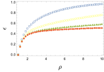
Here, we attempt to overcome this issue by exploiting the properties of the deterministic limit of the model, and by finding a way to close the equations for $\theta$ and $\lambda$ in the finite-$N$ case, while still retaining the essential features of the full model. In order to do this, we start from Eqs. (42)–(43) for the partially reduced $(K+1)$-dimensional deterministic system for $\theta$ and $i_{k}$. Examination of the eigenvalues appearing in Eq. (48), shows that $|\Lambda^{\{K+1\}}|<|\Lambda^{\{2,\ldots,K\}}|$. If the ratio $\epsilon\equiv|\Lambda^{\{K+1\}}/\Lambda^{\{2,\ldots,K\}}|$ is small, then there is the potential to carry out a reduction of the system. In such case, the deterministic dynamics would quickly evolve along the directions corresponding to the set of most negative eigenvalues towards a lower-dimensional region of the state-space, in which the system as a whole evolves in a much slower time-scale, and which contains the fixed point $(\theta^{*},0,\ldots,0)$. As illustrated in Fig. 1, showing the value of $\epsilon$ for different choices of $K$, we would expect this time-scale separation to occur for combinations of parameters for which the final size of the epidemic is small, i.e., for large $\theta^{*}$.

Since there is one most negative eigenvalue, with a degeneracy equal to $(K-1)$, after sufficient time has passed the evolution of the system will then be constrained to a two-dimensional surface, which we will refer to as the slow subspace. With the aim of reducing the dimensionality of the problem, then, we ignore the fast initial behavior of the system and focus the analysis on the slow surface. We do so by imposing the condition that no dynamics exists along the $(K-1)$ fast directions, i.e.,

$$\bm{u}^{\{j\}}\cdot\bm{A}(\bm{x}) =0,\qquad\qquad j=2,\ldots,K,$$ (49)

where $\bm{x}=(\theta,i_{1},\ldots,i_{K})$, and $\bm{u}^{\{j\}}$ is the $j$-th left-eigenvector of the Jacobian $\bm{J}^{\{K+1\}}$ evaluated at the fixed point $(\theta^{*},0,\ldots,0)$, with $\theta^{*}$ given by Eq. (34). This procedure goes under the name of adiabatic elimination, or fast-variable elimination Haken (1983), and it is a common practice in the simplification of deterministic non-linear dynamical systems—e.g., systems of oscillating chemical reactions Tyson (1982); Zhabotinsky and Rovinsky (1987).

Figure 1: Relative magnitudes of $\Lambda^{\{K+1\}}$ and $\Lambda^{\{2,\ldots,K\}}$, $\epsilon=|\rho\phi(\theta^{*})/\langle k^{2}\rangle-1|$, as a function of $\theta^{*}$ for ${\alpha=-2.5}$ and $K=10$ (blue squares), $K=10^{2}$ (empty yellow circles), $K=10^{4}$ (green triangles) and $K=10^{6}$ (filled red circles).

For ease of application of the method, the left- and right-eigenvectors of the Jacobian are normalized in such a way that

$$\bm{u}^{\{i\}}\cdot\bm{v}^{\{j\}} =\delta_{ij};$$ (50)

these are given, respectively, by Eqs. (78) and (80). Imposing the condition given by Eq. (49), one finds that $A_{k+1}=Y_{k}\sum^{K}_{l=1}lA_{l+1}$, where $k=2,\ldots,K$ and $Y_{k}$ is given by Eq. (79). In terms of the $\theta$ and $i_{k}$ variables, this reads

$$i_{k}=\frac{kd_{k}}{\gamma\phi(\theta^{*})}\,\left[\gamma{\theta^{*}}^{k}-\beta\left(\phi(\theta){\theta^{*}}^{k}-\phi(\theta^{*})\theta^{k}\right)\right]\,\sum^{K}_{l=1}li_{l},\ \ k=2,\ldots,K,$$ (51)

and this gives the behavior of $i_{k}$ which limits the dynamics of the deterministic system to a slow subspace. A more convenient form can be found by multiplying Eq. (51) by $k$ and summing from $k=2$ to $k=K$. This allows us to relate $\sum^{K}_{l=1}li_{l}$ to $i_{1}$ to find the following $(K-1)$ expressions for $i_{k}$:

$$i_{k} =\frac{i_{1}}{d_{1}}\frac{1}{\gamma\theta^{*}-\beta\left[\theta^{*}\phi(\theta)-\theta\phi(\theta^{*})\right]}kd_{k}\left[\gamma{\theta^{*}}^{k}-\beta\left(\phi(\theta){\theta^{*}}^{k}-\phi(\theta^{*})\theta^{k}\right)\right],\ \ k=2,\ldots,K.$$ (52)

It should be stressed that the $(K-1)$ equations (52), which we may write in the form $i_{k}(\tau)=F_{k}(\theta(\tau),i_{1}(\tau))$, $k=2,\ldots,K$, should be interpreted as the time-evolution that the $i_{k}$ need to follow, so that $d\bm{x}/d\tau=0$ in the directions $\bm{v}^{\{k\}}$, $k=2,\ldots,K$. This follows from the deterministic equations of motion $d\bm{x}/d\tau=\bm{A}(\bm{x})$ and from Eq. (49). Thus the only temporal evolution is in the $\bm{v}^{\{1\}}$ and $\bm{v}^{\{K+1\}}$ directions.

The functional forms $i_{k}(\tau)=F_{k}(\theta(\tau),i_{1}(\tau))$, with $F_{k}$ defined by Eq. (52), formally only hold sufficiently near the fixed point that linearization is accurate. However in Fig. 2 we show three-dimensional projections of the deterministic dynamics from Eqs. (42)–(43) for an epidemic on a network characterized by a power-law degree distribution with $\alpha=-2.5$ and maximum degree $K=10$, with heterogeneous basic reproductive ratio $\rho=1.2$, which gives $\epsilon\approx 0.184$. It appears that the solid red line, which represents the deterministic dynamics, lies in the slow subspace for most of the time, not just at late times when the system approaches the fixed point. That this is the case can be seen from a consideration of the Jacobian of the system at an arbitrary time, and not just at the fixed point:

$$\bm{J}^{\{K+1\}} =\left(\begin{array}[]{rr}-\beta\sum_{m}mi_{m}&\ -\beta\theta l\\ \\ \beta k^{2}d_{k}\theta^{k-1}\sum_{m}mi_{m}&\ \beta kld_{k}\theta^{k}-\gamma\delta_{kl}\end{array}\right).$$ (56)

It is straightforward to check that $(0,\psi_{1},\ldots,\psi_{K})^{\top}$ is a right-eigenvector of the matrix in Eq. (56) with eigenvalue $-\gamma$, if $\sum^{K}_{l=1}l\psi_{l}=0$. Therefore, remarkably, the eigenvectors $\bm{v}^{\{k\}}$ of the Jacobian at the fixed point, defined in Eq. (78), are eigenvectors of the Jacobian at all times. The existence of this negative eigenvalue with degeneracy $(K-1)$ means that the system remains in the plane described by the vectors $\bm{v}^{\{1\}}$ and $\bm{v}^{\{K+1\}}$, since any small deviations out of the plane will tend to be pushed back again. Normally, when carrying out a fast-variable elimination, one would find that the system possesses a line of fixed points which is quickly approached at early times, dominated by the deterministic dynamics, and along which the slow, stochastic dynamics takes place. In this case, however, the line of fixed points corresponds to an absorbing boundary of the system: the evolution of the epidemic stops altogether once it reaches the disease-free state. Therefore, it is important that the projection onto the slow variables constitutes a good approximation to the dynamics also far from the line of fixed points.

We parameterize the slow subspace using the coordinates $z_{1}\equiv\bm{u}^{\{1\}}\cdot\bm{x}$ and $z_{2}\equiv\bm{u}^{\{K+1\}}\cdot\bm{x}$. Using Eq. (80) and $\bm{x}=(\theta,i_{1},\ldots,i_{K})$, we obtain

$$z_{1} =\theta+\frac{\beta\theta^{*}}{-\gamma+\beta\phi(\theta^{*})}\sum^{K}_{k=1}ki_{k},$$ (57)

$$z_{2} =\frac{Kd_{K}{\theta^{*}}^{K}}{\phi(\theta^{*})}\sum^{K}_{k=1}ki_{k}.$$ (58)

A linear transformation of Eqs. (57) and (58) shows that an equivalent set of coordinates are $\theta$ and $\sum_{k}ki_{k}$, previously called $\lambda$. So, in summary, in Sec. III we showed the system of $2K$ equations leads to a closed set of equations in $\theta$ and $\lambda$. Here, through a consideration of the slow modes of the deterministic equations, we have shown that not only can we describe the system in terms of $\theta$ and $\lambda$, but that it remains in the vicinity of a subspace that can be parameterized by these variables.

Figure 2: Projection of the full epidemic dynamics onto (a) $(\theta,i_{1},i_{2})$, and (b) $(\theta,i_{1},i_{5})$, for $K=10$, $\alpha=-2.5$, $\rho=1.2$, $N=10^{5}$, where $s_{k}=d_{k}\theta^{k}$ and $i_{k}$ are the fractions of susceptible and infected individuals of degree $k$, respectively. Red, dashed line: deterministic limit, Eqs. (42)–(43); blue, yellow, green lines: stochastic differential equations (37) and (8). The initial condition corresponds to $i_{1,0}=0.005$, $i_{k,0}=0$ for $k=2,\ldots,K$, and $G(\theta_{0})=1-i_{1,0}$. In both cases, the system is pushed back from the initial condition (lower right in both panels) towards the slow subspace described by Eq. (52), on which it seems to stay during the rest of the course of the epidemic. Note the different scales in the $z$ axes of both panels, so the fluctuations away from the slow subspace are small in both cases; the fluctuations on the slow subspace can, however, be large, as seen from the departure of the stochastic trajectories from the deterministic dynamics.

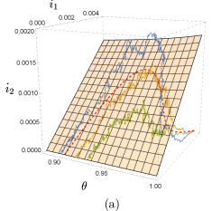
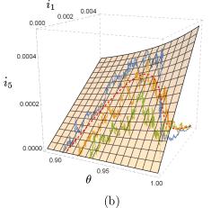
We would like to carry this reasoning over to the stochastic case, to find a reduced set of SDEs, but which are closed, i.e., which can be expressed entirely in terms of the slow variables $z_{1}$ and $z_{2}$ (or $\theta$ and $\lambda$). Before starting the actual treatment of the model, we visualize its dynamics to find whether the system evolves towards a lower-dimensional subspace, as it does in the deterministic case. Figure 2 also shows three-dimensional projections of stochastic trajectories from Eqs. (37) and (8), for a total population of $N=10^{5}$. The behavior is found indeed to be similar to that of the deterministic case: the dynamics seems to quickly reach, and then fluctuate around, the deterministic slow subspace, with the early behavior dominated by the deterministic dynamics. Therefore, we expect that we should be able to effectively reduce the stochastic system from $(K+1)$ dimensions to two dimensions, by neglecting the fast initial behavior of the epidemic.

We will do this by projecting the stochastic differential equations, Eqs. (37) and (8), onto the slow degrees of freedom of the deterministic limit of the model; that is, we will neglect the fluctuations away from the slow subspace, along the $(K-1)$ fast directions corresponding to the most negative eigenvalue. This can be formulated mathematically through the application of a projection operator that only picks the components of $\bm{x}$, $\bm{A}(\bm{x})$, and $\bm{\eta}(\tau)$ along the slow eigenvectors of the deterministic limit, $\bm{v}^{\{1\}}$ and $\bm{v}^{\{K+1\}}~{}$Constable and McKane (2014):

$$\bm{P} =\bm{v}^{\{1\}}[\bm{u}^{\{1\}}]^{\top}+\bm{v}^{\{K+1\}}[\bm{u}^{\{K+1\}}]^{\top}.$$ (59)

The details of the derivation are given in Appendix B, where it is shown that the SDEs given by Eqs. (37) and (41) of Sec. III are recovered, except that now $\bar{\sigma}_{3}\equiv\sqrt{\bar{B}_{33}}$ is determined in terms of $\theta$ and $\lambda$. This closed system of stochastic differential equations for $\theta$ and $\lambda$, which we call the reduced mesoscopic model, constitutes the main result of this paper and so we reproduce it here:

$$\frac{d\theta}{d\tau} =-\beta\theta\lambda+\frac{1}{\sqrt{N}}\bar{\sigma}_{1}\zeta_{1}(\tau),$$ (60)

$$\frac{d\lambda}{d\tau} =\lambda(\beta\phi(\theta)-\gamma)+\frac{1}{\sqrt{N}}\left[-\frac{\phi(\theta)}{\theta}\bar{\sigma}_{1}\zeta_{1}(\tau)+\bar{\sigma}_{2}\zeta_{2}(\tau)+\bar{\sigma}_{3}\zeta_{3}(\tau)\right],$$ (61)

where $\bar{\sigma}_{1}^{2}=\left[G^{\prime}(\theta)\right]^{-1}\beta\lambda\theta$, $\bar{\sigma}_{2}^{2}=\beta\lambda[\phi(\theta)+\psi(\theta)]-\bar{\sigma}^{2}_{1}$, and

$$\bar{\sigma}_{3}^{2} =\lambda\left(\gamma\frac{\phi(\theta^{*})+\psi(\theta^{*})}{\phi(\theta^{*})}+\frac{\beta}{\phi(\theta^{*})}\left[\phi(\theta^{*})\psi(\theta)-\phi(\theta)\psi(\theta^{*})\right]\right).$$ (62)

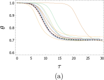
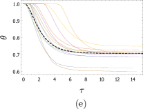
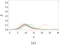
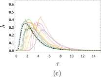
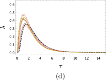
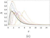
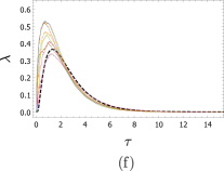
We now compare the dynamics of the full microscopic model, defined by Eqs. (1)–(3), to that of the reduced mesoscopic model above. Figures 3 and 4 show the time series of the full microscopic model in terms of the variables $\theta$ and $\lambda$, and that of the reduced mesoscopic model, for $N=20000$ and different values of $K$ having the same deterministic final size $\theta^{*}$, obtained from Eq. (34); Figure 5, in turn, compares the phase diagrams. We see that, in the case of small $K$, the time series of both variables in the full microscopic model are rather smooth, and are dominated by a horizontal spread due to the fact that the epidemic takes off at different moments. As heterogeneity increases, the dynamics of the system becomes noisier and noisier, as seen in the phase diagrams; however, the time series of $\theta$ continues to be smooth. This observation will be useful in the following section.

From the time series of the reduced mesoscopic model we see that, except for small $K$, the temporal behavior of $\theta$ and $\lambda$ does not present the horizontal spread observed in the full microscopic model. However, once the epidemic has taken off, the dynamics of the full microscopic model is correctly captured when $K$ is not so large; this can be seen from the phase diagrams. We note that the relative magnitude of the eigenvalues for this choice of parameters takes the values $\epsilon\approx 0.44\text{--}0.65$, and that the reduced mesoscopic model fares well despite $\epsilon$ being rather large. We find slightly worse agreement between the full and reduced models for smaller values of $\theta^{*}$, corresponding to larger $\epsilon$. One further detail to add is that in the case of the reduced model there are far fewer trajectories in which the epidemic does take off, compared to the full microscopic model; that is, the reduced model results in an over-representation of very early extinctions.

Note that, for the value of $N$ employed in these figures, $K=19999$ is the maximum possible degree cutoff. In this case, we would not expect the reduced model to yield accurate results. This is due to the fact that not even the full $2K$-dimensional mesoscopic model (Eqs. (7)–(8)) provides a good approximation to the microscopic dynamics in this case, since $K$ is of the order of $N$ and this would need to be explicitly taken into account when performing the mesoscopic expansion leading to the Fokker-Planck equation (4). The implementation of the reduced mesoscopic model, however, is much more practical than that of the full mesoscopic model: while we have found that simulations of the latter take a time that, as its number of equations, grows linearly with the degree of heterogeneity of the network, for the reduced version this time, besides being much shorter, appears to scale as $\sqrt{K}$.

We end this section with some further observations regarding the reduced stochastic system. First, the existence of a $(K-1)$-fold degenerate eigenvalue equal to $-\gamma$ throughout the time evolution also means that stochastic trajectories, as well as deterministic ones, which venture out of the slow subspace will tend to be pushed back into the plane. Thus we would expect the reduced set of SDEs to be a good approximation throughout the motion, and not just at late times. This may be the reason why the approximation works well even if $\epsilon$ is not particularly small. Second, in retrospect, the elimination of the fast variables in the stochastic system is not strictly necessary, since the SDEs previously obtained in Sec. III are recovered, and $\bar{\sigma}_{3}$ could be found in terms of $\theta$ and $\lambda$ using Eq. (52) obtained from the elimination of fast variables in the deterministic system. One can compare the value of $\bar{\sigma}_{3}$ in terms of the $i_{k}$ to the one in terms of $\lambda$ in the deterministic limit and see that, indeed, the approximation is not very good for moderate to large values of $\epsilon$. This does not seem to play a huge role when considered as one of many terms in the stochastic evolution of $\lambda$.

Finally, we can make a general comment about the nature of the fluctuations as the epidemic starts to grow from its initial state. In this case the relevant eigenvalues will be those of the Jacobian Eq. (56), but with $i_{k}=0$ and $\theta=1$, and will therefore be given by those in Eq. (48), but with $\theta^{*}$ set equal to $1$. Therefore, the largest eigenvalue is now $(\rho-1)\gamma$. In this case, if $\rho>1$, so that an epidemic starts to grow, the dynamics is pushed away from the line $(\theta,0,\ldots,0)$ in its early stages, as can be seen from Fig. 2, where the trajectories leave the vicinity of the absorbing state after reaching the slow subspace.

Figure 3: Time series of $\theta$ for $N=20000$, $\gamma=1$, and $\theta^{*}=0.7$, with (a)–(b) $K=10$, (c)–(d) $K=1000$, and (e)–(f) $K=19999$. Colored lines correspond to realizations of the full microscopic model (left panels) and the reduced mesoscopic model (60)–(61) (right panels) started with a total number of 5 infectives with degrees sampled from a truncated Zipf distribution with $\alpha=-2.5$. The black, dashed line corresponds to the deterministic solution.

Figure 4: Time series of $\lambda$ for $N=20000$, $\gamma=1$, and $\theta^{*}=0.7$, with (a)–(b) $K=10$, (c)–(d) $K=1000$, and (e)–(f) $K=19999$. Colored lines correspond to realizations of the full microscopic model (left panels) and the reduced mesoscopic model (60)–(61) (right panels) started with a total number of 5 infectives with degrees sampled from a truncated Zipf distribution with $\alpha=-2.5$. The black, dashed line corresponds to the deterministic solution.

Figure 5: Phase diagrams for $N=20000$, $\gamma=1$, and $\theta^{*}=0.7$, for (a)–(c) the full microscopic model, and (d)–(f) the reduced mesoscopic model (60)–(61). Colored lines correspond to stochastic realizations started with a total number of 5 infectives with degrees sampled from a truncated Zipf distribution with $\alpha=-2.5$ and $K=10$ (left), $K=1000$ (center), and $K=19999$ (right). The black, dashed line corresponds to the deterministic solution.

V Further reduction

In the previous section, we have derived a reduced two-dimensional system with three white-noise processes, the reduced mesoscopic model Eqs. (60)–(61), which provides a good approximation to the dynamics of the full microscopic model, provided the maximum degree individuals can pick is not so large. This is true even for relatively large values of $\epsilon$, corresponding to small separation between the eigenvalues of the system. We have also noted that the time series of $\theta$, obtained from the full microscopic model, presents very smooth behavior over the range of parameters explored. Inspired by this observation, we attempt to further simplify the model by noting that Eqs. (60)–(61) have the form

$$\frac{d\theta}{d\tau} =-\beta\theta\lambda+\sqrt{\frac{\lambda}{N}}f_{1}(\theta)\zeta_{1}(\tau),$$ (63)

$$\frac{d\lambda}{d\tau} =\lambda\left(\beta\phi(\theta)-\gamma\right)-\sqrt{\frac{\lambda}{N}}f_{2}(\theta)\zeta_{1}(\tau)+\sqrt{\frac{\lambda}{N}}f_{3}(\theta)\zeta_{2}(\tau)+\sqrt{\frac{\lambda}{N}}f_{4}(\theta)\zeta_{3}(\tau).$$ (64)

Figure 6: Relative intensities of the noise terms in Eqs. (63)–(64) for (a)–(c) $\theta^{*}=0.7$, and (d)–(f) $\theta^{*}=0.9$, with $K=10$ (left), $K=1000$ (center), $K=19999$ (right). Blue, solid line: $f=f_{2}$; yellow, dashed line: $f=f_{3}$; green, dot-dashed line: $f=f_{4}$.

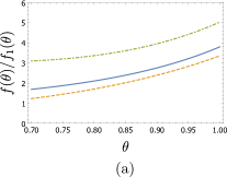
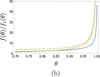
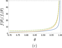
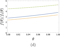
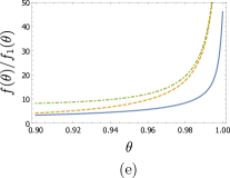
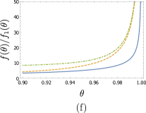
Taking into account the fact that, in any given realization of the process, the lowest value reached by $\theta$ will be roughly around $\theta^{*}$, we compare the magnitudes of the noise intensities $f_{1},\ldots,f_{4}$ between $\theta=\theta^{*}$ and $\theta=1$ for fixed $\theta^{*}$ and different values of $K$. We find that, in general, and especially during the early stages of the epidemic when $\theta\approx 1$, $f_{1}$ is small compared to $f_{2},f_{3}$ and $f_{4}$—see Fig. 6; the effect is more pronounced for more heterogeneous distributions with smaller deterministic final sizes, i.e., larger $\theta^{*}$. Therefore, the system may be described simply by a deterministic ordinary differential equation (ODE) for $\theta$, and Eqs (60)–(61) become

$$\frac{d\theta}{d\tau} =-\beta\theta\lambda,$$ (65)

$$\frac{d\lambda}{d\tau} =\lambda\left(\beta\phi(\theta)-\gamma\right)+\frac{1}{\sqrt{N}}\bar{\sigma}\zeta(\tau),$$ (66)

with $\zeta(\tau)$ a Gaussian noise with zero mean and $\langle\zeta(\tau)\zeta(\tau^{\prime})\rangle=\delta(\tau-\tau^{\prime})$, with the noise intensity, $\bar{\sigma}$, given by

$$\bar{\sigma} =\left[\left(\frac{\phi(\theta)}{\theta}\right)^{2}\bar{\sigma}_{1}^{2}+\bar{\sigma}_{2}^{2}+\bar{\sigma}_{3}^{2}\right]^{1/2}.$$ (67)

We call this system the semi-deterministic mesoscopic model, which is two-dimensional like the reduced mesoscopic model, but has only one white-noise process in place of the latter’s three. Here we have used that $\langle\zeta_{\mu}(\tau)\rangle=0$, and $\langle\zeta_{\mu}(\tau)\zeta_{\nu}(\tau^{\prime})\rangle=\delta_{\mu\nu}\delta(\tau-\tau^{\prime})$, $\mu,\nu=1,2,3$. Now, we note that Eq. (66) corresponds to a Cox-Ingersoll-Ross (CIR) model Cox et al. (1985),

$$\frac{d\lambda}{d\tau} =a(\theta(\tau))(b-\lambda)d\tau+\sigma(\theta(\tau))\sqrt{\lambda}\zeta(\tau),$$ (68)

where $\theta(\tau)$ is a time-dependent parameter that is the solution of the deterministic differential equation (65), $b=0$, and

$$a(\theta(\tau)) =\gamma-\beta\phi(\theta(\tau)),$$ (69)

$$\sigma(\theta(\tau)) =\frac{1}{\sqrt{N}}\sqrt{\beta\left[\phi(\theta(t))\left(1-\frac{\psi(\theta^{*})}{\phi(\theta^{*})}\right)+2\psi(\theta(t))\right]+\gamma\frac{\phi(\theta^{*})+\psi(\theta^{*})}{\phi(\theta^{*})}}.$$ (70)

For fixed $a$ and $\sigma$, the conditional probability distribution of $\lambda(\tau+\Delta\tau)=\lambda$, given $\lambda(\tau)=\lambda^{\prime}$, is known in closed form, and corresponds to a non-central chi-square distribution given by Cox et al. (1985); Feller (1951)

$$P(\lambda,\tau+\Delta\tau|\lambda^{\prime},\tau) =ce^{-u-v}\left(\frac{v}{u}\right)^{q/2}I_{q}(2\sqrt{uv}),$$ (71)

where

$$\begin{array}[]{rclcrcl}c&\equiv&\dfrac{2a}{\sigma^{2}\left(1-e^{-a\Delta\tau}\right)},&&u&\equiv&\displaystyle c\lambda^{\prime}\,e^{-a\Delta\tau},\\ v&\equiv&\displaystyle c\lambda,&&q&\equiv&\dfrac{2ab}{\sigma^{2}}-1=-1,\end{array}$$ (74)

and where $I_{q}$ is the modified Bessel function of the first kind of order $q$.

Therefore, if we assume that $\theta$ evolves discretely, staying constant from time $\tau$ to time $\tau+\Delta\tau$ for reasonably small $\Delta\tau$, we can use the result above to simulate Eqs. (65)–(66) by sampling the values of $\lambda$ directly from the distribution in Eq. (71) with fixed parameters $a(\theta(\tau))$, $\sigma(\theta(\tau))$ at every time-step. The case $b=0$ corresponds to the special case of a non-central chi-square distribution with zero degrees of freedom; thus, in order to simulate Eq. (66) we follow the method described in Refs. Glasserman (2003); Andersen et al. (2010) and sample from a central chi-square distribution with Poisson-distributed degrees of freedom, with the convention that the central chi-square distribution with zero degrees of freedom is identically zero Siegel (1979). Figure 7 shows the dynamics obtained in this way. While we note an additional over-representation of early extinctions, the other results are in very good agreement with the reduced mesoscopic model, Eqs. (60)–(61).

Figure 7: Phase diagrams from the semi-deterministic mesoscopic model with $N=20000$, $\gamma=1$, and $\theta^{*}=0.7$. Colored lines correspond to realizations of Eqs. (65)–(66), started with a total number of 5 infectives with degrees sampled from a truncated Zipf distribution with $\alpha=-2.5$ and (a) $K=10$, (b) $K=1000$, and (c) $K=19999$. The black, dashed line corresponds to the deterministic solution.

VI Distribution of epidemic sizes

In the previous sections, we have derived a two-dimensional reduction of the $2K$-dimensional SIR dynamics described by Eqs. (7)–(8), by exploiting a separation of time-scales in the deterministic dynamics of the system. We have found reasonably good agreement between the temporal behaviors of the full and reduced models. Furthermore, we have also discussed an extra simplification, consisting in neglecting the noise acting on the susceptible variable $\theta$, and describing the system in terms of one ODE and one SDE instead of two SDEs. Now we explore how accurately these reductions capture the distribution of epidemic sizes, given by the number of recovered individuals present in the system at the end of the epidemic, $r_{\infty}$, which can be obtained as $r_{\infty}=1-\sum_{k}s_{k,\infty}$ and $r_{\infty}=1-G(\theta_{\infty})$ in the full and reduced models, respectively, where $s_{k,\infty}$ and $\theta_{\infty}$ are the final values of $s_{k}$ and $\theta$—not to be confused with the fixed points in the deterministic limit, $s_{k}^{*}$ and $\theta^{*}$. Formal mathematical work has considered central limit theorems for models that generalize ours Neal (2007); we are interested here in explicit calculation and simulation approaches.

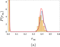
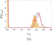
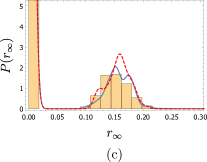
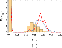
We obtain the distribution of $r_{\infty}$ from the full model via a Sellke construction House (2014), and note that it is characterized by two regions: one to the left of the interval, corresponding to early extinctions, and one to the right corresponding to the epidemic taking off. The first thing we note when comparing this to results from the two versions of the reduced model—Eqs.(60)–(61), and Eqs. (65)–(66)—is that, as discussed previously, there is an over-representation of very early extinctions in the case of the latter, and therefore the relative sizes of the left- and right-most regions of the distribution are not well captured. We would not expect our diffusion approximation to capture extinction probabilities accurately, given that its derivation implicitly assumes that the infective population is large and extinctions by definition involve small numbers of infectives. We can, however, derive accurate extinction probabilities from other results we have obtained.

First, we make an argument related to ‘susceptibility sets’ in probability Ball (2000). For each pair of individuals in the population, we pick whether infection will be spread between them if one becomes infective and draw a link between them if it will. This forms a static graph, and if we pick a node of the graph to be initially infective, then the size of the epidemic will be the size of the network component that the initial pick is part of. This means that the size of the giant component of the graph is equal to the final size of the epidemic if it is large, and the probability of early extinction is equal to the proportion of the population in the small components of this graph. Therefore, we can conclude that we have already calculated the probability of early extinction of the epidemic starting with an individual picked uniformly at random from a very large population; it will be equal to $\sum_{k}s_{k}^{*}=G(\theta^{*})$.

Figure 8 shows the distribution of final sizes from the reduced and semi-deterministic mesoscopic models, adjusted to account for the inaccuracy in early extinctions by removing these and assuming that a fraction $G(\theta^{*})$ of epidemics stop early, and a fraction $1-G(\theta^{*})$ take the values from the mesoscopic models. These results are compared to the distribution from the full model and show that the argument we have introduced provides a simple method to adjust for the inaccuracies in early extinctions, yielding an accurate approximation overall.

Figure 8: Distribution of epidemic sizes for $N=20000$, $\alpha=-2.5$ and $\gamma=1$, for (a)–(b) $\theta^{*}=0.7$, and (c)–(d) $\theta^{*}=0.9$, with $K=1000$ (left panels) and $K=19999$ (right panels). Histogram: full model; blue, solid line: reduced mesoscopic model Eqs. (60)–(61); red, dashed line: semi-deterministic mesoscopic model Eqs. (65)–(66).

VII Discussion

Stochastic epidemics on heterogeneous networks involve two potentially large parameters. The first of these is the size of the population, $N$, which is proportional to the dimensionality of the microscopic description. For large populations, this motivates the derivation of a mesoscopic model based on a diffusion approximation whose errors are controlled by inverse powers of $N$, and which we have formulated in this paper. The second of these is the maximum degree $K$, which is proportional to the dimensionality of the full mesoscopic model. We have been able to use fast-mode elimination techniques to derive two-dimensional approximations to this scheme: the reduced mesoscopic model, which involves three white-noise processes; and the semi-deterministic mesoscopic model, which involves only one white-noise process.

Our numerical results back up our theoretical understanding that these low-dimensional systems are accurate approximations to the microscopic model, except in the case where $K$ approaches $N$, although this is to be expected since our derivation of the diffusion limit implicitly assumes that $K\ll N$. Nevertheless, the reduction can be applied to cases with extremely large values of $K$, as long as they are not too close to $N$, thus significantly simplifying the original model.

We have observed that the elimination of fast variables in the system provides a good approximation to the full dynamics even for relatively large values of $\epsilon$, corresponding to a small separation between time-scales. We have also shown that the main inaccuracy of the reduction, relating to very early extinction probabilities of the epidemic, can be dealt with using a simple argument. In this way, we hope to have provided a useful tool in the study of both infectious diseases and spreading processes on heterogeneous networks.

Appendix A Eigenvectors of the deterministic system

Full system

A set of right-eigenvectors corresponding to the eigenvalues from Eq. (16) are given by

$$\begin{split}\bm{v}^{\{k\}}&=\bm{e}_{k},\qquad k=1,\ldots,K,\\ \bm{v}^{\{k\}}&=\bm{e}_{3K+1-k}-(2K+1-k)\bm{e}_{K+1},\qquad k=K+1,\ldots,2K-1,\\ \bm{v}^{\{2K\}}&=-X\sum_{k=1}^{K}ks^{*}_{k}\bm{e}_{k}+\sum_{k=1}^{K}ks^{*}_{k}\bm{e}_{K+k},\end{split}$$ (75)

where $\bm{e}_{i}$ is the $i$-th unit vector and

$$X=\frac{\beta\sum_{k=1}^{K}k^{2}s^{*}_{k}}{\beta\sum_{k=1}^{K}k^{2}s^{*}_{k}-\gamma}.$$ (76)

Totally reduced system

A set of right-eigenvectors corresponding to the eigenvalues from Eq. (28) are given by

$$\begin{split}\bm{v}^{\{1\}}&=\left(1,0\right)^{\top},\\ \bm{v}^{\{2\}}&=\left(-\frac{\beta\theta^{*}}{\beta\phi(\theta^{*})-\gamma},1\right)^{\top}.\end{split}$$ (77)

Partially reduced system

The partially reduced system with eigenvalues given by Eq. (48) has a set of right-eigenvectors given by

$$\begin{split}\bm{v}^{\{1\}}&=\bm{e}_{1},\\ \bm{v}^{\{k\}}&=\bm{e}_{K+3-k}-(K+2-k)\bm{e}_{2},\qquad k=2,\ldots,K,\\ \bm{v}^{\{K+1\}}&=\frac{1}{Y_{K}}\left(\sum_{k=1}^{K}Y_{k}\bm{e}_{k+1}-X\bm{e}_{1}\right),\end{split}$$ (78)

where now

$$\begin{split}X&=\frac{\beta\theta^{*}}{\beta\phi(\theta^{*})-\gamma},\\ Y_{k}&=\frac{kd_{k}{\theta^{*}}^{k}}{\phi(\theta^{*})}.\end{split}$$ (79)

In Eqs. (75) and (77) we did not normalize the eigenvectors. However, in this case we do need the eigenvectors to be normalized to simplify the application of the reduction technique described in Sec. IV. This requires finding the corresponding left-eigenvectors. When finding these, we have a complication given by the fact that there is one eigenvalue which is $(K-1)$-fold degenerate, and the condition (50) will not necessarily hold in general. However, if we construct a matrix $\bm{V}$ in such a way that its $i$-th column corresponds to $\bm{v}^{\{i\}}$, we can choose $\bm{u}^{\{j\}}$ to be the $j$-th row of the inverse matrix $\bm{V}^{-1}$, if such an inverse exists. We find that indeed this is the case, and the left-eigenvectors in the partially reduced model are then given by

$$\begin{split}\bm{u}^{\{1\}}&=\bm{e}_{1}+X\sum_{k=1}^{K}k\bm{e}_{k+1},\\ \bm{u}^{\{k\}}&=\bm{e}_{K+3-k}-Y_{K+2-k}\sum_{l=1}^{K}l\bm{e}_{l+1},\qquad k=2,\ldots,K,\\ \bm{u}^{\{K+1\}}&=Y_{K}\sum_{k=1}^{K}k\bm{e}_{k+1}.\end{split}$$ (80)

We note that

$$\sum_{k=1}^{K}kY_{k} =\frac{\sum_{k=1}^{K}k^{2}d_{k}{\theta^{*}}^{k}}{\phi(\theta^{*})}=\frac{\phi(\theta^{*})}{\phi(\theta^{*})}=1.$$ (81)

Using this property, we can verify that the orthogonality condition (50) is satisfied:

$$\begin{split}\bm{u}^{\{1\}}\cdot\bm{v}^{\{1\}}&=1,\\ \bm{u}^{\{1\}}\cdot\bm{v}^{\{j\}}&=(K+2-j)X-(K+2-j)X=0,\qquad j=2,\ldots,K,\\ \bm{u}^{\{1\}}\cdot\bm{v}^{\{K+1\}}&=-\frac{X}{Y_{K}}+\frac{X}{Y_{K}}\sum_{k=1}^{K}kY_{k}=0,\\ \bm{u}^{\{i\}}\cdot\bm{v}^{\{1\}}&=0,\qquad i=2,\ldots,K,\\ \bm{u}^{\{i\}}\cdot\bm{v}^{\{j\}}&=\delta_{ij}+Y_{K+2-i}(K+2-j)-Y_{K+2-i}(K+2-j)=\delta_{ij},\qquad i,j=2,\ldots,K,\\ \bm{u}^{\{i\}}\cdot\bm{v}^{\{K+1\}}&=\frac{Y_{K+2-i}}{Y_{K}}-\frac{Y_{K+2-i}}{Y_{K}}\sum_{k=1}^{K}kY_{k}=0,\qquad i=2,\ldots,K,\\ \bm{u}^{\{K+1\}}\cdot\bm{v}^{\{1\}}&=0,\\ \bm{u}^{\{K+1\}}\cdot\bm{v}^{\{j\}}&=Y_{k}(K+2-j)-Y_{k}(K+2-j)=0,\qquad j=2,\ldots,K,\\ \bm{u}^{\{K+1\}}\cdot\bm{v}^{\{K+1\}}&=\sum_{k=1}^{K}kY_{k}=1.\end{split}$$ (82)

Appendix B Fast-variable elimination

In this Appendix we derive the two-dimensional reduced mesoscopic model, by projecting the dynamics of the ${(K+1)}$-dimensional partially reduced mesoscopic model onto the slow degrees of freedom of its corresponding deterministic limit.

Using the projector defined in Eq. (59) on $\bm{x}=(\theta,i_{1},\ldots,i_{K})$ gives the slow variables defined by Eqs. (57) and (58). Later, the inverse transformation, back to the more familiar variables $\theta$ and $\sum_{k}ki_{k}(=\lambda)$, will be required. It is

$$\theta(\bm{z}) =z_{1}-\frac{\beta z_{2}\phi(\theta^{*})}{K{\theta^{*}}^{K-1}d_{K}\left[-\gamma+\beta\phi(\theta^{*})\right]},$$ (83)

$$\lambda(\bm{z}) =\frac{\phi(\theta^{*})}{Kd_{K}{\theta^{*}}^{K}}\,z_{2},$$ (84)

however for the moment we will use the $z_{1}$ and $z_{2}$ variables, and will denote the right-hand side of Eq. (83) as $\chi(\bm{z})$.

The deterministic slow dynamics, obtained by applying the projector to $\bm{A}(\bm{x})$, will be given by

$$\dot{z}_{1} =\frac{\phi(\theta^{*})}{Kd_{K}{\theta^{*}}^{K}}\beta z_{2}\left[-\chi(\bm{z})+\frac{\theta^{*}\left(\beta\phi(\chi(\bm{z}))-\gamma\right)}{-\gamma+\beta\phi(\theta^{*})}\right],$$ (85)

$$\dot{z}_{2} =z_{2}\left(\beta\phi(\chi(\bm{z}))-\gamma\right),$$ (86)

where the dot represents the time derivative.

Applying now the projector to the noise terms in the finite-$N$ case we find, for the component along $\bm{v}^{\{1\}}$,

$$\eta_{z_{1}}(\tau) =\frac{1}{\sqrt{N}}\bm{u}_{1}\cdot\left(\frac{1}{G^{\prime}(\theta)}\sum_{k}\sigma_{1}^{(k)}\rho_{1}^{(k)}(\tau),-\sigma_{1}^{(1)}\rho_{1}^{(1)}(\tau)+\sigma_{2}^{(1)}\rho_{2}^{(1)}(\tau),\ldots,-\sigma_{1}^{(K)}\rho_{1}^{(K)}(\tau)+\sigma_{2}^{(K)}\rho_{2}^{(K)}(\tau)\right)$$

$$=\frac{1}{\sqrt{N}}\left[\xi_{1}(\tau)+\frac{\beta\theta^{*}}{-\gamma+\beta\phi(\theta^{*})}\left(\xi_{2}(\tau)+\xi_{3}(\tau)\right)\right]$$ (87)

$$=\frac{1}{\sqrt{N}}\left[\left(1-\frac{\phi(\chi(\bm{z}))}{\chi(\bm{z})}\frac{\beta\theta^{*}}{-\gamma+\beta\phi(\theta^{*})}\right)\bar{\sigma}_{1}(\bm{z})\zeta_{1}(\tau)+\frac{\beta\theta^{*}}{-\gamma+\beta\phi(\theta^{*})}\left(\bar{\sigma}_{2}(\bm{z})\zeta_{2}(\tau)+\bar{\sigma}_{3}(\bm{z})\zeta_{3}(\tau)\right)\right],$$ (88)

where we obtain, from Eqs. (52), (57) and (58),

$$\bar{\sigma}_{1}(\bm{z}) =\left[\frac{\beta\phi(\theta^{*})z_{2}\chi(\bm{z})}{Kd_{K}{\theta^{*}}^{K}G^{\prime}(\chi(\bm{z}))}\right]^{1/2},$$ (89)

$$\bar{\sigma}_{2}(\bm{z}) =\left[\frac{\beta\phi(\theta^{*})z_{2}}{Kd_{K}{\theta^{*}}^{K}}\left(\phi(\chi(\bm{z}))+\psi(\chi(\bm{z}))-\frac{\phi(\chi(\bm{z}))^{2}}{\chi(\bm{z})G^{\prime}(\chi(\bm{z}))}\right)\right]^{1/2},$$ (90)

$$\bar{\sigma}_{3}(\bm{z}) =\left[\frac{z_{2}}{Kd_{K}{\theta^{*}}^{K}}\left(\gamma\left[\phi(\theta^{*})+\psi(\theta^{*})\right]+\beta\left[\phi(\theta^{*})\psi(\chi(\bm{z}))-\phi(\chi(\bm{z}))\psi(\theta^{*})\right]\right)\right]^{1/2}.$$ (91)

Similarly, for the component of the fluctuations along $\bm{v}^{\{K+1\}}$:

$$\eta_{z_{2}}(\tau) =\frac{1}{\sqrt{N}}\frac{Kd_{K}{\theta^{*}}^{K}}{\phi(\theta^{*})}\left(-\frac{\phi(\chi(\bm{z}))}{\chi(\bm{z})}\bar{\sigma}_{1}(\bm{z})\zeta_{1}(\tau)+\bar{\sigma}_{2}(\bm{z})\zeta_{2}(\tau)+\bar{\sigma}_{3}(\bm{z})\zeta_{3}(\tau)\right).$$ (92)

We now form $\dot{\theta}$ and $\dot{\lambda}$ as linear combinations of $\dot{z}_{1}$ and $\dot{z}_{2}$, using Eqs. (83) and (84). These are equal to the appropriate linear combinations of Eqs. (85), (86), (88), and (92). One finds that Eqs. (37) and (41) are exactly recovered, except that now $\bar{\sigma}_{3}\equiv\sqrt{\bar{B}_{33}}$ is determined, given by Eq. (91).

References

- Rock et al. (2014) K. Rock, S. Brand, J. Moir, and M. J. Keeling, Rep. Prog. Phys. 77, 026602 (2014).
- Heesterbeek et al. (2015) H. Heesterbeek, R. M. Anderson, V. Andreasen, S. Bansal, D. De Angelis, C. Dye, K. T. D. Eames, W. J. Edmunds, S. D. W. Frost, S. Funk, T. D. Hollingsworth, T. House, V. Isham, P. Klepac, J. Lessler, J. O. Lloyd-Smith, C. J. E. Metcalf, D. Mollison, L. Pellis, J. R. C. Pulliam, M. G. Roberts, C. Viboud, and Isaac Newton Institute IDD Collaboration, Science 347, aaa4339 (2015).
- Danon et al. (2011) L. Danon, A. P. Ford, T. House, C. P. Jewell, M. J. Keeling, G. O. Roberts, J. V. Ross, and M. C. Vernon, Interdisc. Perspect. Infect. Diseases 2011 (2011), article ID 284909.
- Pastor-Satorras et al. (2015) R. Pastor-Satorras, C. Castellano, P. Van Mieghem, and A. Vespignani, Rev. Mod. Phys. 87, 925 (2015).
- Pellis et al. (2015) L. Pellis, F. Ball, S. Bansal, K. Eames, T. House, V. Isham, and P. Trapman, Epidemics 10, 58 (2015).
- Bailey (1957) N. T. J. Bailey, The Mathematical Theory of Epidemics (Griffin, London, 1957).
- Anderson and May (1991) R. M. Anderson and R. M. May, Infectious Diseases of Humans (Oxford University Press, Oxford, 1991).
- King et al. (2015) A. A. King, M. Domenech de Cellès, F. M. G. Magpantay, and P. Rohani, Proc. R. Soc. B 282, 20150347 (2015).
- Britton et al. (2015) T. Britton, T. House, A. L. Lloyd, D. Mollison, S. Riley, and P. Trapman, Epidemics 10, 54 (2015).
- Keeling and Rohani (2007) M. J. Keeling and P. Rohani, Modeling Infectious Diseases in Humans and Animals (Princeton University Press, New Jersey, 2007).
- Diekmann et al. (1990) O. Diekmann, J. A. P. Heesterbeek, and J. A. J. Metz, J. Math. Biol. 28, 365 (1990).
- Miller et al. (2012) J. C. Miller, A. C. Slim, and E. M. Volz, J. R. Soc. Interface 9, 890 (2012).
- Eames and Keeling (2002) K. T. D. Eames and M. J. Keeling, Proc. Nat. Acad. Sci. (USA) 99, 13330 (2002).
- May and Anderson (1988) R. M. May and R. M. Anderson, Philos. Trans. R. Soc. London B 321, 565 (1988).
- Ferreira et al. (2012) S. C. Ferreira, C. Castellano, and R. Pastor-Satorras, Phys. Rev. E 86, 041125 (2012).
- House (2014) T. House, Math. Model. Nat. Phenom. 9, 153 (2014).
- Leigh Brown et al. (2011) A. J. Leigh Brown, S. J. Lycett, L. Weinert, G. J. Hughes, E. Fearnhill, and D. T. Dunn, J. Infect. Dis. 204, 1463 (2011).
- House et al. (2015) T. House, J. M. Read, L. Danon, and M. J. Keeling, EPJ Data Sciece 4, 13 (2015).
- Pastor-Satorras and Vespignani (2001) R. Pastor-Satorras and A. Vespignani, Phys. Rev. E 63, 066117 (2001).
- May and Lloyd (2001) R. M. May and A. L. Lloyd, Phys. Rev. E 64, 066112 (2001).
- Pastor-Satorras and Vespignani (2002) R. Pastor-Satorras and A. Vespignani, Phys. Rev. E 65, 035108 (2002).
- Berger et al. (2005) N. Berger, C. Borgs, J. T. Chayes, and A. Saberi, in Proceedings of the 16th Annual ACM-SIAM Symposium on Discrete Algorithms (Society for Industrial and Applied Mathematics, Philadelphia, PA, 2005) pp. 301–310.
- Durrett (2010) R. Durrett, Proc. Nat. Acad. Sci. (USA) 107, 4491 (2010).
- Hong et al. (2007) H. Hong, M. Ha, and H. Park, Phys. Rev. Lett. 98, 258701 (2007).
- Boguñá et al. (2009) M. Boguñá, C. Castellano, and R. Pastor-Satorras, Phys. Rev. E 79, 036110 (2009).
- Graham and House (2014) M. Graham and T. House, J. Math. Biol. 68, 1583 (2014).
- McKane et al. (2014) A. J. McKane, T. Biancalani, and T. Rogers, Bull. Math. Biol. 76, 895 (2014).
- Rozhnova et al. (2011) G. Rozhnova, A. Nunes, and A. J. McKane, Phys. Rev. E 84, 051919 (2011).
- Rozhnova et al. (2012) G. Rozhnova, A. Nunes, and A. J. McKane, Phys. Rev. E 85, 051912 (2012).
- van Kampen (2007) N. G. van Kampen, Stochastic Processes in Physics and Chemistry, 3rd ed. (Elsevier Science, Amsterdam, 2007).
- Gillespie (1976) D. T. Gillespie, J. Comput. Phys. 22, 403 (1976).
- Gillespie (1992) D. T. Gillespie, Markov Processes: An Introduction for Physical Scientists (Academic Press, San Diego, 1992).
- Gardiner (2009) C. W. Gardiner, Handbook of Stochastic Methods, 4th ed. (Springer, Berlin, 2009).
- Volz (2008) E. M. Volz, J. Math. Biol. 56, 293 (2008).
- House and Keeling (2010) T. House and M. J. Keeling, J. R. Soc. Interface 8, 67 (2010).
- Miller (2011) J. C. Miller, J. Math. Biol. 62, 349 (2011).
- Miller and Volz (2013) J. C. Miller and E. M. Volz, PLOS ONE 8, e69162 (2013).
- Haken (1983) H. Haken, Synergetics (Springer, Berlin, 1983).
- Tyson (1982) J. J. Tyson, J. Phys. Chem. 86, 3006 (1982).
- Zhabotinsky and Rovinsky (1987) A. M. Zhabotinsky and A. B. Rovinsky, J. Stat. Phys. 48, 959 (1987).
- Constable and McKane (2014) G. W. A. Constable and A. J. McKane, Phys. Rev. E 89, 032141 (2014).
- Cox et al. (1985) J. C. Cox, J. E. Ingersoll Jr, and S. A. Ross, Econometrica 53, 385 (1985).
- Feller (1951) W. Feller, Ann. Math. 54, 173 (1951).
- Glasserman (2003) P. Glasserman, Monte Carlo Methods in Financial Engineering, Vol. 53 (Springer Science & Business Media, New York, 2003) Chapter 3.
- Andersen et al. (2010) L. B. Andersen, P. Jäckel, and C. Kahl, “Simulation of square-root processes,” in Encyclopedia of Quantitative Finance (John Wiley & Sons, New York, 2010).
- Siegel (1979) A. F. Siegel, Biometrika 66, 381 (1979).
- Neal (2007) P. Neal, J. Appl. Probab. 44, 41 (2007).
- Ball (2000) F. G. Ball, “Susceptibility sets and the final outcome of stochastic SIR epidemic models,” Research Report 00-09, Division of Statistics, School of Mathematical Sciences, University of Nottingham, (2000).