The distribution of first hitting times
of non-backtracking random walks
on Erdős-Rényi networks

Abstract

We present analytical results for the distribution of first hitting times of non-backtracking random walks on finite Erdős-Rényi networks of $N$ nodes. The walkers hop randomly between adjacent nodes on the network, without stepping back to the previous node, until they hit a node which they have already visited before or get trapped in a dead-end node. At this point, the path is terminated. The length, $d$, of the resulting path, is called the first hitting time. Using recursion equations, we obtain analytical results for the tail distribution of first hitting times, $P(d>\ell)$, $\ell=0,1,2,\dots$, of non-backtracking random walks starting from a random initial node. It turns out that the distribution $P(d>\ell)$ is given by a product of a discrete Rayleigh distribution and an exponential distribution. We obtain analytical expressions for central measures (mean and median) and a dispersion measure (standard deviation) of this distribution. It is found that the paths of non-backtracking random walks, up to their termination at the first hitting time, are longer, on average, than those of the corresponding simple random walks. However, they are shorter than those of self avoiding walks on the same network, which terminate at the last hitting time. We obtain analytical results for the probabilities, $p_{\rm ret}$ and $p_{\rm trap}$, that a path will terminate by retracing, namely stepping into an already visited node, or by trapping, namely entering a node of degree $k=1$, which has no exit link, respectively. It is shown that in dilute networks the dominant termination scenario is trapping while in dense networks most paths terminate by retracing. We obtain expressions for the conditional tail distributions of path lengths, $P(d>\ell|{\rm ret})$ and $P(d>\ell|\rm{trap})$, for those paths which terminate by retracing or by trapping, respectively. We also study a class of generalized non-backtracking random walk models which not only avoid the backtracking step into the previous node but avoid stepping into the last $S$ visited nodes, where $S=2,3,\dots,N-2$. Note that the case of $S=1$ coincides with the non-backtracking random walk model described above, while the case of $S=N-1$ coincides with the self avoiding walk.

Keywords: Random network, Erdős-Rényi network, degree distribution, random walk, self-avoiding walk, first hitting time

1 Introduction

Random walk (RW) models [1, 2] are useful for the study of a large variety of stochastic processes such as diffusion [3, 4], polymer structure [5, 6] and random search [7, 8]. These models were studied extensively in geometries including continuous space [9], regular lattices [10], fractals [11] and random networks [12]. A RW on a network hops randomly at each time step to one of the nodes which are adjacent to the current node. Thus, if the current node is of degree $k$, the probability of each one of its neighbors to be selected by the RW is $1/k$. In some of the steps the RW hops into new nodes, which have not been visited before. In other steps it may backtrack its path into the previous node or hop into nodes already visited at earlier times. It was found that RWs on random networks are highly effective in exploring the network, retracing their steps much less frequently than RWs on low dimensional lattices [13]. Recent studies of random walks on random networks produced analytical results for the mean first passage time between random pairs of nodes [14], the average number of distinct nodes visited by a RW after $t$ time steps [15] and the mean cover time [16].

A special type of random walk model, which has been studied extensively on regular lattices, is the self avoiding walk (SAW). This is a random walk which does not visit the same node more than once [17]. At each time step, the walker chooses its next move randomly from the neighbors of its present node, excluding nodes that were already visited. The path terminates when the RW reaches a dead-end node from which it cannot exit, namely a node which does not have any yet unvisited neighbors. The length of the path, $d$, is given by the number of steps made until the path has terminated. The path length of an SAW on a connected network of size $N$ can take values between $1$ and $N-1$. The latter case corresponds to a Hamiltonian path [18]. More specifically, the SAW path lengths between a given pair of nodes, $i$ and $j$, are distributed in the range bounded from below by the shortest path length between these nodes [19, 20] and from above by the longest non-overlapping path between them [21]. The path length of an SAW on a random network is called the last hitting time [22]. In Ref. [23] we presented analytical results for the distribution of SAW path lengths, or last hitting times, on ER networks [24, 25, 26]. These SAW paths are often referred to as kinetic growth self-avoiding walks [27], or true self avoiding walks [28]. This is in contrast to SAW paths which are uniformly sampled among all possible self avoiding paths of a given length. It was found that the distribution of SAW path lengths follows a discrete version of the Gompertz distribution [29, 30, 31, 32]. This means that the SAWs exhibit a termination rate per step which increases exponentially with the number of steps already pursued.

Another important time scale which appears in random walks on networks is the first hitting time [15], also referred to as the first intersection length [33, 34]. This time scale emerges in a class of RW models which are not restricted to be self avoiding. In these models the RW hops freely between adjacent nodes until it enters a node which has already been visited before. At this point the path is terminated. The number of time steps up to termination of the path, which coincides with the path length, is called the first hitting time. This time, on average, is much smaller than the last hitting time, namely the path length of an SAW on the same network. This is due to the fact that the RW path may terminate at any time step, $t>1$, by randomly hopping into an already visited node, even if the current node has one or more yet-unvisited neighbors. This is in contrast with the SAW path, which terminates only when the current node does not have any yet-unvisited neighbors. In Ref. [35] we presented analytical results for the distribution of first hitting times of RWs on ER networks. In the analysis, we utilized the fact that up to its termination the RW follows an SAW path. The path pursued by the RW may terminate either by backtracking into the previous node or by retracing itself, namely stepping into a node which was already visited two or more time steps earlier. By calculating the probabilities of these two termination scenarios, we obtained analytical results for the distribution of first hitting times of RWs on ER networks. We also obtained analytical results for the probabilities, $p_{\rm backtrack}$ and $p_{\rm ret}$, that a RW, starting from a random initial node, will terminate by backtracking or by retracing, respectively. It was found that in dilute networks most paths terminate by backtracking while in dense networks most paths terminate by retracing.

The RW model studied in Ref. [35] and the SAW model studied in Ref. [23] are very different from each other. The SAW may be considered as a walker which maintains a complete record of all the nodes it has visited and avoids stepping into any of them again. On the other hand, the RW does not keep track of its path and thus may hop into an already visited node at any time step. This difference leads to different termination scenarios in the two models. While the RW path is terminated by either backtracking or by retracing of its own path, the SAW terminates only when it reaches a dead end node which does have any yet unvisited neighbor. The RW model and the SAW model can be considered as two opposite limits in a class of RW models which keep track of the last $S$ visited nodes, where $S=0,1,\dots,N-1$, and avoid stepping into any of them again. Put differently, in the $t+1$ time step such RW avoids hopping from the current node, to which entered at time $t$, into any of the nodes visited at times $t-1$, $t-2$, $\dots$, $t-S$, even if they are adjacent to the current node. However, it may hop into nodes visited at earlier times, in which case the path is terminated. The case of $S=0$ corresponds to the RW studied in Ref. [35]. The case of $S=1$ corresponds to the non-backtracking random walk (NBW), which avoids hopping back into the previous node. RW models with $S>1$ are called generalized NBW models, which are closely related to a class of models known as tourist walks [36, 37]. Note that the case of $S=N-1$ coincides with the SAW model studied in Ref. [23].

The paths of NBWs have been studied on regular lattices and random graphs [38]. It was shown that they explore the network more efficiently than RWs. It was also shown that they mix faster, namely require a shorter transient time to reach the stationary distribution of visiting frequencies throughout the network. The path of the NBW model studied here may terminate either by retracing, namely by hopping into a node which has already been visited before, or by trapping, namely entering a dead-end node from which it cannot exit.

NBWs provide a useful description of a large variety of randomly wandering objects on networks. These objects are endowed with a memory, which enables them to avoid revisiting the nodes visited in the last $S$ time steps. The non-backtracking property is often highly beneficial. For example, it speeds-up the performance of web-crawlers which constantly scan the world-wide-web. Also, it extends the life expectancy of random foragers which feed on the network.

Web crawlers are robots which scan the internet and assemble information from webpages, to be used in search engines and other databases [39]. They hop randomly in the web following the hyperlinks. To optimize the efficiency of web crawlers it is important to avoid revisiting sites at too high frequency. On the other hand, web crawlers need to keep the information fresh, namely revisit web sites frequently enough to account for updates. A generalized NBW protocol provides a strategy for such web crawlers, because tuning the parameter $S$ enables to balance between these competing requirements.

To make the connection to foraging theory, consider an animal, which is randomly foraging in a random network environment. Each time the animal visits a node it consumes all the food available in this node and needs to move on to one of the adjacent nodes. The model describes rather harsh conditions, in which the regeneration of resources is very slow and the visited nodes do not replenish within the lifetime of the forager. Moreover, the forager does not carry any reserves and in order to survive it must hit a vital node each and every time. Under these conditions, the distribution of life expectancies of the foragers coincides with the distribution of first hitting times. Clearly, a forager which avoids hopping back to the previous node (thus described by an NBW model) will have a higher life expectancy than a forager which may hop back to the previous node (described by an RW model). Foragers which avoid revisiting the last $S$ visited nodes are described by the generalized NBW model. Their life expectancy further increases as $S$ is increased.

Several variants of the forager model have been studied on lattices of different dimensions. For example, the case in which the forager carries sufficient resources which enable it to avoid starvation even when it visits several non-replenished nodes in a row, was recently studied [40, 41]. The effect of the regeneration rate of the visited nodes was also examined. It was shown that under slow regeneration the forager is susceptible to starvation, while above some threshold regeneration rate, the probability of starvation diminishes [42].

In this paper we present analytical results for the distribution of first hitting times of NBWs on ER networks. We obtain expressions for the mean, median and standard deviation of this distribution in terms of the parameters of the network. It turns out that the termination of an NBW path may occur either by the retracing scenario or by trapping in a dead-end (leaf) node, from which it cannot exit. We obtain analytical results for the probabilities, $p_{\rm ret}$ and $p_{\rm trap}$, that an NBW will terminate by retracing or by trapping, respectively. It is found that in dilute networks most paths terminate by trapping while in dense networks most paths terminate by retracing. We also obtain expressions for the conditional tail distributions of path lengths, $P(d>\ell|{\rm ret})$ and $P(d>\ell|{\rm trap})$, given that the NBWs are terminated by retracing or by trapping, respectively. We show that as $S$ is increased, the termination probability decreases and the mean path length increases.

The paper is organized as follows. In Sec. 2 we describe the class of non-backtracking random walk models on the ER network. In Sec. 3 we consider the evolution of the subnetwork which consists of the yet unvisited nodes. In Sec. 4 we derive analytical results for the distribution of path lengths, or first hitting times, of NBWs on ER networks. In Sec. 5 we obtain analytical expressions for two central measures (mean and median) and a dispersion measure (standard deviation) of this distribution. In Sec. 6 we analyze the distributions of path lengths of NBWs, conditioned on the termination scenario. In Sec. 7 we consider generalized NBW models and present analytical results for the distribution of first hitting times in these models. The results are summarized and discussed in Sec. 8. The details of the calculations of $P(d>\ell)$ for the NBW model and for the generalized NBW model are presented in Appendices A and B, respectively. The calculation of the mean of $P(d>\ell)$ for the generalized NBW model is presented in Appendix C.

2 The non-backtracking random walk models

Consider a random walk on a random network of $N$ nodes, starting from a random initial node. Each time step the walker chooses randomly one of the neighbors of its current node, and hops to the chosen node. The RW continues to hop between adjacent nodes as long as it does not visit any node more than once. For concreteness, we denote the initial node by $x_{0}$ and the subsequent nodes along the path by $x_{t}$, $t=1,2,\dots$, where $x_{t}$ is the node which the RW enters at time $t$ and leaves at time $t+1$. The RW path is terminated upon the first time it steps into an already visited node. The resulting path length is referred to as the first hitting time or the first intersection length.

The NBW may hop randomly to any neighbor of the current node, except for the previous node, from which it entered the current node. This significantly reduces the termination probability because the previous node is the only node which is guaranteed to be connected to the current node. The NBW exhibits two termination scenarios, namely retracing and trapping. In the retracing scenario, the NBW hops into an already visited node. In the trapping scenario it hops into a dead end (leaf) node of degree $k=1$, from which the only way out is by backtracking, which is not allowed.

We also consider generalized NBW models, which keep track of the last $S$ visited nodes and avoid hopping into them. The parameter, $S$, may take values in the range $1\leq S\leq N-1$. The case of $S=1$ is the NBW model, in which backtracking into the previous node is not allowed. The paths of NBWs may terminate either by hopping into nodes already visited at earlier times (retracing) or by trapping in a leaf node of degree $k=1$ from which they cannot exit. Generalized NBW models, with $S>1$, avoid hopping into any of the nodes visited at times $t=1$, $t-2$, $\dots$, $t-S$. The paths of generalized NBWs may terminate either by retracing or by trapping in a node which is surrounded by the tail of $S$ nodes which they cannot enter. The case of $S=N-1$ coincides with the SAW model.

3 Evolution of the subnetwork of the yet-unvisited nodes

Consider an $ER(N,p)$ network. The degree $k_{i}$ of node $i=1,\dots,N$ is the number of links connected to this node. The degree distribution $p(k)$ of the ER network is a binomial distribution, which in the sparse limit ($p\ll 1$) is approximated by a Poisson distribution of the form

$$p(k)=\frac{{c}^{k}}{k!}e^{-c},$$ (1)

where $c=(N-1)p$ is the average degree. In the asymptotic limit ($N\rightarrow\infty$), the ER network exhibits a phase transition at $c=1$ (a percolation transition), such that for $c<1$ the network consists only of small clusters and isolated nodes, while for $c>1$ there is a giant cluster which includes a macroscopic fraction of the network, in addition to small clusters and isolated nodes. At $c=\ln N$, there is a second transition, above which the entire network is included in the giant cluster and there are no isolated components.

Here we focus on the regime above the percolation transition, namely $c>1$. For $1<c<\ln N$ the fraction of isolated nodes among all nodes in the network is given by $i(c)=\exp(-c)$. In order to avoid the trivial case of an NBW starting on an isolated node, we performed the analysis presented below for the case in which the initial node is non-isolated. At time steps $t=2,\dots,S+1$ the generalized NBW avoids hopping into any of the previously visited nodes, and thus behaves as an SAW. At $t\geq S+2$, it avoids hopping from the node it entered at time $t-1$ into the nodes visited at times $t-2$, $t-3$, $\dots$, $t-S-1$ but may hop into nodes visited at earlier times, thus causing termination of the path. In these models, as long as the path does not terminate, it is identical to an SAW path.

The NBW path divides the network into two subnetworks, one consists of the already visited nodes and the other consists of the yet-unvisited nodes. After $t$ time steps the size of the subnetwork of visited nodes is $t+1$ (including the initial node), while the size of the network of yet-unvisited nodes is $N(t)=N-t-1$. We denote the degree distribution of the subnetwork of the yet-unvisited nodes at time $t$ by $p_{t}(k)$, $k=0,\dots,N(t)-1$, where $p_{0}(k)=p(k)$, namely the original degree distribution. The average degree of this subnetwork is given by

$$\langle k\rangle_{t}=\sum_{k=0}^{N(t)-1}kp_{t}(k).$$ (2)

We denote it by $c(t)=\langle k\rangle_{t}$, where $c(0)=c$.

RWs on random networks exhibit higher probabilities of visiting nodes of high degrees. More precisely, the probability that in a given time step a RW will visit a node of degree $k$, is given by $kp(k)/c$, namely it is proportional to the degree of the node. A special property of the Poisson distribution is that the probability ${kp(k)}/{c}=p(k-1)$. This means that, the probability that the node visited at time $t+1$ will be of degree $k$ is given by $p(k-1)$. In Ref. [23] it was shown that the degree distribution of the subnetwork which consists of the yet unvisited nodes at time $t$ is

$$p_{t}(k)=\frac{c(t)^{k}}{k!}e^{-c(t)},$$ (3)

where

$$c(t)=\left(1-\frac{t}{N-1}\right)c$$ (4)

is the mean degree of this subnetwork. This means that the subnetwork of the yet-unvisited nodes remains an ER network, while its size and mean degree decrease linearly in time. Therefore, the degree distribution of this subnetwork also satisfies ${kp_{t}(k)}/{c(t)}=p_{t}(k-1)$.

4 The distribution of first hitting times of the NBW model

Consider an NBW (with $S=1$) on an ER network of $N$ nodes. The NBW starts from a random node with degree $k\geq 1$ (non-isolated node) and hops randomly between nearest neighbor nodes without backtracking into the previous node. The path of the NBW may terminate either by the retracing scenario or by the trapping scenario. In the retracing mechanism the NBW steps into a node which was already visited two or more time steps earlier. In the trapping mechanism the NBW enters a dead end (leaf) node of degree $k=1$ from which it cannot exit.

In case that the NBW has pursued $t$ steps, without retracing its path and without getting trapped, the path length, $d$, is guaranteed to satisfy $d>t-1$. At this point, the probability that the path will not terminate in the $t+1$ step is denoted by the conditional probability $P(d>t|d>t-1)$. This conditional probability can be expressed as a product of the form

$$P(d>t|d>t-1)=P_{\rm ret}(d>t|d>t-1)P_{\rm trap}(d>t|d>t-1).$$ (5)

The conditional probability $P_{\rm trap}(d>t|d>t-1)$ is the probability that the NBW will not terminate by the trapping scenario at the $t+1$ time step. Given that the NBW is not terminated by trapping at the $t+1$ step, the conditional probability $P_{\rm ret}(d>t|d>t-1)$ is the probability that it will also not terminate by the retracing scenario, namely that it will not step into a node already visited at an earlier time.

The probability that the NBW will not terminate by the trapping mechanism in the $t+1$ time step is given by the probability that the node it entered at time $t$ is of degree $k>1$. This probability is given by

$$P_{\rm trap}(d>t|d>t-1)=\sum_{k=2}^{N-1}\frac{kp(k)}{c}.$$ (6)

Inserting in Eq. (6) the Poisson distribution of Eq. (1) we obtain

$$P_{\rm trap}(d>t|d>t-1)=1-e^{-c}.$$ (7)

Note that this probability does not depend on the time, $t$. Given that the NBW was not terminated by trapping at the $t+1$ time step, we will now evaluate the probability, $P_{\rm ret}(d>t|d>t-1)$, that it will also not terminate by retracing. Apart from the current node and the previous node, there are $N-2$ possible nodes which may be connected to the current node, each one of them with probability $p$. The fact that the possibility of trapping was already eliminated for the $t+1$ step, guarantees that at least one of these $N-2$ nodes is connected to the current node (otherwise, the only possible move would have been to hop back to the previous node). This leaves $N-3$ nodes such that each one of them is connected to the current node with probability $p$. Thus, the expectation value of the number of neighbors of the current node, to which the NBW may hop in the $t+1$ time step, is $(N-3)p+1$. Due to the local tree-like structure of ER networks, it is extremely unlikely that the one node which is guaranteed to be connected to the current node has already been visited. This is due to the fact that the path from such earlier visit of this adjacent node all the way to the current node is essentially a loop. Therefore, we conclude that this adjacent node has not yet been visited. Since the number of yet unvisited nodes is $N-t-1$, we conclude that the current node is expected to have $(N-t-2)p+1$ neighbors which have not yet been visited. As a result, the probability that the RW will hop into one of the yet-unvisited nodes is given by

$$P_{\rm ret}(d>t|d>t-1)=\frac{(N-t-2)p+1}{(N-3)p+1}.$$ (8)

Inserting $c=(N-1)p$ and $c(t)=(N-t-1)p$ we obtain

$$P_{\rm ret}(d>t|d>t-1)=\frac{c(t)-p+1}{c-2p+1}.$$ (9)

In the asymptotic limit this expression can be approximated by

$$P_{\rm ret}(d>t|d>t-1)=\frac{c(t)+1}{c+1}.$$ (10)

Combining the results presented above, it is found that the probability that the path of the NBW will not terminate at the $t+1$ time step is given by the conditional probability

$$P(d>t|d>t-1)=\left[\frac{c(t)-p+1}{c-2p+1}\right]\left(1-e^{-c}\right).$$ (11)

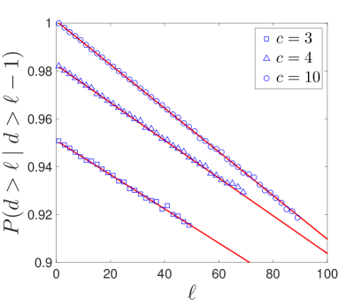
In Fig. 1 we present the conditional probability $P(d>t|d>t-1)$ vs. $t$ for an NBW on an ER network of size $N=1000$ and three values of $c$. The analytical results (solid lines) obtained from Eq. (11) are found to be in very good agreement with numerical simulations (symbols), confirming the validity of this equation. Note that the numerical results become more noisy as $t$ increases, due to diminishing statistics, and eventually terminate. This is particularly apparent for the smaller values of $c$.

Figure 1: Theoretical results (solid lines) for the conditional probability $P(d>\ell|d>\ell-1)$ vs. $\ell$, obtained from Eq. (11), and the results obtained from computer simulations (symbols) of NBWs on ER networks of size $N=1000$ and mean degrees $c=3$, $4$ and $10$ (squares, triangles and circles, respectively). The analytical and numerical results are found to be in very good agreement.

The probability that the path length of the NBW will be longer than $\ell$ is given by

$$P(d>\ell)=P(d>0)\prod_{t=1}^{\ell}P(d>t|d>t-1),$$ (12)

where $P(d>0)=1$, since the initial node is not isolated. Using Eq. (5) the probability $P(d>\ell)$ can be written as a product of the form

$$P(d>\ell)=P_{\rm ret}(d>\ell)P_{\rm trap}(d>\ell),$$ (13)

where

$$P_{\rm trap}(d>\ell)=\prod_{t=1}^{\ell}\left(1-e^{-c}\right),$$ (14)

and

$$P_{\rm ret}(d>\ell)=\prod_{t=1}^{\ell}\left[\frac{c(t)-p+1}{c-2p+1}\right].$$ (15)

In Appendix A we evaluate the probabilities $P_{\rm trap}(d>\ell)$, given by Eq. (14) and $P_{\rm ret}(d>\ell)$, given by Eq. (15). Combining the results for $P_{\rm trap}(d>\ell)$ and for $P_{\rm ret}(d>\ell)$ we obtain

$$\ln[P(d>\ell)] \simeq \left(\ell-\frac{1}{2}-\alpha^{2}\right)\ln\left(1-\frac{\ell-1/2}{\alpha^{2}}\right)-(\beta+1)\ell$$ (16)

$$+ \left(\alpha^{2}-\frac{1}{2}\right)\ln\left(1-\frac{1}{2\alpha^{2}}\right)+1,$$

where

$$\alpha=\sqrt{\frac{N\left(c+1\right)}{c}},$$ (17)

and

$$\beta=-\ln\left(1-e^{-c}\right).$$ (18)

Assuming that the NBW paths are short compared to the network size, namely $\ell\ll N$, one can use the expansion

$$\ln\left(1-\frac{x}{\alpha^{2}}\right)\simeq-\frac{x}{\alpha^{2}}-\frac{1}{2}\left(\frac{x}{\alpha^{2}}\right)^{2}+O\left(\frac{x^{3}}{\alpha^{6}}\right).$$ (19)

Plugging this approximation in Eq. (16) yields

$$P\left(d>\ell\right)\simeq\exp\left[-\frac{\ell(\ell-1)}{2\alpha^{2}}-\beta\ell\right].$$ (20)

Thus, the distribution of path lengths is a product of an exponential distribution and a Rayleigh distribution, which is a special case of the Weibull distribution [43]. Considering the next order in the series expansion of Eq. (19) we find that the relative error in Eq. (20) for $P(d>\ell)$ due to the truncation of the Taylor expansion after the second order is $\eta_{\rm TE}=\ell^{3}/(6\alpha^{4})$, which scales like $\ell^{3}/N^{2}$. This error is very small as long as $\ell\ll N^{1/2}$. Note that paths of length $\ell\simeq N^{1/2}$, for which the error in $P(d>\ell)$ is noticeable, become prevalent only in the limit of dense networks, where $c>N^{1/2}$. The probability density function $P(d=\ell)$ can be obtained by

$$P\left(d=\ell\right)=P\left(d>\ell-1\right)-P\left(d>\ell\right).$$ (21)

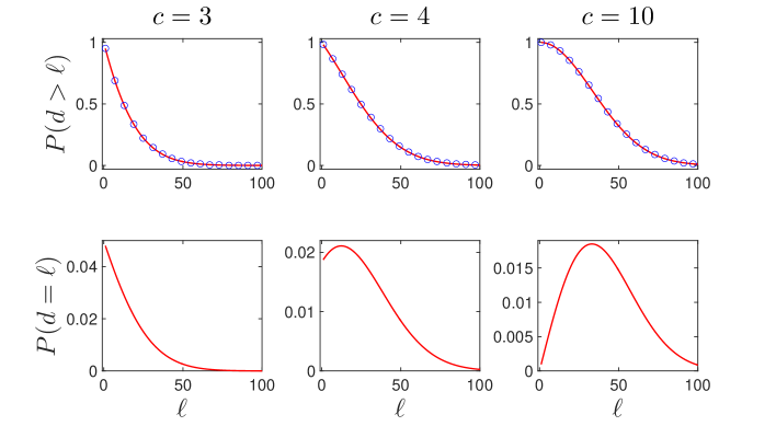
In Fig. 2 we present the tail distributions $P(d>\ell)$ vs. $\ell$ of first hitting times of NBWs on ER networks of size $N=1000$ and mean degrees $c=3$, $4$ and $10$ (top row). The theoretical results (solid lines) were obtained from Eq. (16). They are found to be in excellent agreement with the numerical simulations (symbols). The corresponding probability density functions, $P(d=\ell)$, obtained from Eqs. (16) and (21), are shown in the bottom row.

Figure 2: The tail distributions, $P(d>\ell)$, of the first hitting times of NBWs, vs. $\ell$, for ER networks of size $N=1000$ and $c=3$, $4$ and $10$. The theoretical results (solid lines), obtained from Eq. (16) are found to be in excellent agreement with the results obtained from numerical simulations (circles). The corresponding probability density functions, $P(d=\ell)$, obtained from Eqs. (16) and (21), are shown in the bottom row. The agreement with the numerical results is already established in the top row and therefore the numerical data is not shown in the bottom row.

5 Central and dispersion measures

In order to characterize the distribution of first hitting times of NBWs on ER networks we derive expressions for the mean and median of this distribution. The mean of the distribution can be obtained from the tail-sum formula

$$\ell_{\rm mean}(N,c)=\sum_{\ell=0}^{N-2}P(d>\ell).$$ (22)

Assuming that the initial node is not isolated and expressing the sum as an integral we obtain

$$\ell_{\rm mean}(N,c)\simeq 1+\int_{1/2}^{N-3/2}P(d>\ell)d\ell,$$ (23)

where the limits of the integration are set such that the summation over each integer, $i$, is replaced by an integral over the range $(i-1/2,i+1/2)$. Inserting $P(d>\ell)$ from Eq. (20) and solving the integral we obtain

$$\ell_{\rm mean}=1+\sqrt{\frac{\pi}{2}}\alpha e^{\frac{(\alpha^{2}\beta-1)\beta}{2}}\left[{\rm erf}\left(\frac{\alpha^{2}\beta+N-2}{\sqrt{2}\alpha}\right)-{\rm erf}\left(\frac{\alpha\beta}{\sqrt{2}}\right)\right].$$ (24)

where ${\rm erf}(x)$ is the error function, also called Gauss error function. This function exhibits a sigmoid shape. For $|x|\ll 1$ it can be approximated by ${\rm erf}(x)\simeq 2x/\sqrt{\pi}$ while for $|x|>1$ it quickly converges to ${\rm erf}(x)\rightarrow{\rm sign}(x)$. While the arguments of both ${\rm erf}$ functions in Eq. (24) are large, the argument of the first ${\rm erf}$ function is much larger than the argument of the second. Therefore, one can safely set the first ${\rm erf}$ function to be equal to $1$, and obtain

$$\ell_{\rm mean}\simeq 1+\sqrt{\frac{\pi}{2}}\alpha e^{\frac{(\alpha^{2}\beta-1)\beta}{2}}\left[1-{\rm erf}\left(\frac{\alpha\beta}{\sqrt{2}}\right)\right].$$ (25)

In Fig. 3(a) we present the mean, $\ell_{\rm mean}$, of the distribution of first hitting times of NBWs as a function of the mean degree $c$, for ER networks of size $N=1000$. The agreement between the theoretical results, obtained from Eq. (25) and the numerical simulations is very good for all values of $c$.

Figure 3: The mean $\ell_{mean}$ (a), the median $\ell_{median}$ (b) and the standard deviation $\sigma_{\ell}$ (c), of the distribution of first hitting times of NBWs, as a function of the mean degree, $c$, for ER networks of size $N=1000$. The analytical results (solid lines), obtained from Eqs. (25), (26) and (30), respectively, are in excellent agreement with numerical simulations (circles). For comparison, we also present analytical (dashed lines) and numerical ($\times$) results for the mean, $\ell_{mean}$ (a), the median, $\ell_{median}$ (b) and the standard deviation, $\sigma_{\ell}$ (c), of the distribution of first hitting times of RWs on the same network. Unlike the NBWs, in which the three measures sharply increase and then saturate as $c$ is increased, in case of the RW they rise gradually.

To obtain a more complete characterization of the distribution of first hitting times, it is also useful to evaluate its median, $\ell_{\rm median}$. Here the median is defined as the value of $\ell$ for which

$$|P(d>\ell)-P(d<\ell)|\rightarrow{\rm min},$$ (26)

where $\ell$ may take either an integer or a half-integer value. In Fig. 3(b) we present the median, $\ell_{\rm median}$, of the distribution of first hitting times of NBWs as a function of the mean degree $c$, for ER networks of size $N=1000$. The agreement between the theoretical results and the numerical simulations is very good for all values of $c$.

The moments of the distribution of NBW path lengths, $\langle\ell^{n}\rangle$, are given by the tail-sum formula [44]

$$\langle\ell^{n}\rangle=\sum_{\ell=0}^{N-2}[(\ell+1)^{n}-\ell^{n}]P(d>\ell).$$ (27)

Using this formula to evaluate the second moment and replacing the sum by an integral we obtain

$$\langle\ell^{2}\rangle=1+\int_{\frac{1}{2}}^{N-\frac{3}{2}}\left(2\ell+1\right)\exp\left[-\frac{\ell(\ell-1)}{2\alpha^{2}}-\beta\ell\right]d\ell.$$ (28)

As in Eq. (24), the solution of this integral consists of two ${\rm erf}$ functions. For $N\gg 1$ one can approximate the upper limit of the first error function by $1$, replace $N-3/2$ by $N$ and neglect the term $\exp(-N^{2})$, to obtain

$$\langle\ell^{2}\rangle\simeq 1+2\alpha^{2}e^{-\frac{\beta}{2}}+\sqrt{2\pi}\alpha\left(1-\alpha^{2}\beta\right)e^{(\alpha^{2}\beta-1)\beta/2}\left[1-{\rm erf}\left(\frac{\alpha\beta}{\sqrt{2}}\right)\right].$$ (29)

The standard deviation, $\sigma_{\ell}(c)$, of the distribution of path lengths is thus given by

$$\sigma_{\ell}^{2}(c)=\langle\ell^{2}\rangle-(\ell_{\rm mean})^{2},$$ (30)

where $\langle\ell^{2}\rangle$ is given by Eq. (29) and $\ell_{mean}$ is given by Eq. (25).

In Fig. 3(c) we present the standard deviation, $\sigma_{\ell}(c)$ of the distribution of first hitting times of NBWs as a function of the mean degree, $c$, for ER networks of size $N=1000$. The agreement between the theoretical results, obtained from Eq. (30), and the numerical simulations is very good for all values of $c$.

6 Analysis of the two termination mechanisms

The NBW model studied here may terminate either by the trapping scenario or by the retracing scenario. The trapping mechanism may occur starting from the second step of the NBW. The probability of trapping is $\exp(-c)$ at any time step afterwards, regardless of the number of steps already pursued. The termination by retracing takes place when the NBW steps into a node which it has already visited before. In this case, the path forms a loop which starts at the first visit to the termination node and ends in the second visit. Termination by the retracing scenario may occur starting from the third time step of the NBW. The probability that the NBW will terminate due to retracing increases in time. This is due to the fact that each visited node becomes a potential termination site. It is thus expected that paths that terminate after a small number of steps are likely to terminate by trapping, while paths which survive for a long time are more likely to terminate by retracing. Below we present a detailed analysis of the probabilities of an NBW to terminate by trapping or by retracing.

Consider an NBW on an ER network, which starts from a random, non-isolated node, hops to a new node at each of the first $\ell$ time steps, and terminates at the $\ell+1$ step. Since the termination step is not counted as a part of the path, the length of such NBW path is $d=\ell$. The probability distribution function of the NBW path lengths, $P(d=\ell)$, is given by Eq. (21). We denote by $p_{\rm trap}$ the probability that an NBW starting from a random initial node will eventually terminate by the trapping scenario and by $p_{\rm ret}$ the probability that it will terminate by the retracing scenario. Since these are the only two termination mechanisms in the NBW model, the two probabilities must satisfy $p_{\rm trap}+p_{\rm ret}=1$.

While the overall distribution of path lengths is given by $P(d=\ell)$, one expects the distribution $P(d=\ell|{\rm trap})$, of paths terminated by trapping, to differ from the distribution $P(d=\ell|{\rm ret})$, of paths terminated by retracing. These conditional probability distributions are normalized, namely they satisfy

$$\sum_{t=1}^{N-1}P(d=t|{\rm trap})=1,$$ (31)

and

$$\sum_{t=2}^{N-1}P(d=t|{\rm ret})=1.$$ (32)

The distribution of path lengths can be expressed in terms of the conditional distributions according to

$$P(d=\ell)=p_{\rm trap}P(d=\ell|{\rm trap})+p_{\rm ret}P(d=\ell|{\rm ret}).$$ (33)

The first term on the right hand side of Eq. (33) can be written as

$$p_{\rm trap}P(d=\ell|{\rm trap})=P(d>\ell-1)\left[1-P_{\rm trap}(d>\ell|d>\ell-1)\right],$$ (34)

namely as the probability that the RW will pursue $\ell$ steps and will terminate at the $\ell+1$ step by the trapping scenario. The second term on the right hand side of Eq. (33) can be written as

$$p_{\rm ret}P(d=\ell|r)=P(d>\ell-1)P_{\rm trap}(d>\ell|d>\ell-1)\left[1-P_{\rm ret}(d>\ell|d>\ell-1)\right],$$ (35)

namely as the probability that the RW will pursue $\ell$ steps, then in the $\ell+1$ step it will not get trapped but will retrace its path by stepping into a node which was already visited at least two steps earlier.

Summing up both sides of Eq. (34) over all integer values of $\ell$ we obtain

$$p_{\rm trap}=e^{-c}\sum_{\ell=1}^{N-1}P(d>\ell-1).$$ (36)

Using the tail-sum formula, Eq. (22), we find that the probability that the NBW will terminate by the trapping scenario is

$$p_{\rm trap}=e^{-c}\ell_{\rm mean}.$$ (37)

Therefore, the probability of the NBW to terminate by retracing its path is

$$p_{\rm ret}=1-e^{-c}\ell_{\rm mean}.$$ (38)

Using Eq. (34) the conditional probability $P(d=\ell|{\rm trap})$ can be written in the form

$$P(d=\ell|{\rm trap})=\frac{P(d>\ell-1)}{\ell_{\rm mean}},$$ (39)

where $P(d>\ell-1)$ is given by Eq. (20). Similarly, the conditional probability $P(d=\ell|{\rm ret})$ takes the form

$$P(d=\ell|{\rm ret})=\left(\frac{1-e^{-c}}{c+1}\right)\left[\frac{c-c(\ell)}{1-e^{-c}\ell_{\rm mean}}\right]P(d>\ell-1),$$ (40)

where $c(\ell)$ is given by Eq. (4). The corresponding tail distributions take the form

$$P(d>\ell|{\rm trap})=\frac{\sum\limits_{t=\ell+1}^{N-1}P(d>t-1)}{\ell_{\rm mean}},$$ (41)

and

$$P(d>\ell|{\rm ret})=\left(\frac{1-e^{-c}}{c+1}\right)\sum\limits_{t=\ell+1}^{N-1}\left[\frac{c-c(t)}{1-e^{-c}\ell_{\rm mean}}\right]P(d>t-1).$$ (42)

Given that the path of an NBW terminated after $\ell$ steps, it is interesting to evaluate the conditional probabilities $P({\rm trap}|d=\ell)$ and $P({\rm ret}|d=\ell)$, that the termination was caused by trapping or by retracing, respectively. Using Bayes’ theorem, these probabilities can be expressed by

$$P({\rm trap}|d=\ell)=\frac{p_{\rm trap}P(d=\ell|{\rm trap})}{P(d=\ell)}$$ (43)

and

$$P({\rm ret}|d=\ell)=\frac{p_{\rm ret}P(d=\ell|{\rm ret})}{P(d=\ell)}.$$ (44)

Clearly, these distributions satisfy $P({\rm trap}|d=\ell)+P({\rm ret}|d=\ell)=1$. Inserting the conditional probabilities $P(d=\ell|{\rm trap})$ and $P(d=\ell|{\rm ret})$ from Eqs. (39) and (40), respectively, we find that

$$P({\rm trap}|d=\ell)=\frac{P(d>\ell-1)}{e^{c}P(d=\ell)}$$ (45)

and

$$P({\rm ret}|d=\ell)=\left(1-e^{-c}\right)\frac{\left[c-c(\ell)\right]}{(c+1)}\frac{P(d>\ell-1)}{P(d=\ell)}.$$ (46)

The corresponding tail distributions can be expressed in the form

$$P({\rm trap}|d>\ell)=\frac{\sum\limits_{t=\ell+1}^{N-1}P(d>t-1)}{e^{c}P(d>\ell)}$$ (47)

and

$$P({\rm ret}|d>\ell)=\left(\frac{1-e^{-c}}{c+1}\right)\sum_{t=\ell+1}^{N-1}\left[c-c(t)\right]\frac{P(d>t-1)}{P(d>\ell)}.$$ (48)

These distributions also satisfy $P({\rm trap}|d>\ell)+P({\rm ret}|d>\ell)=1$.

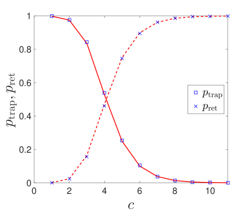
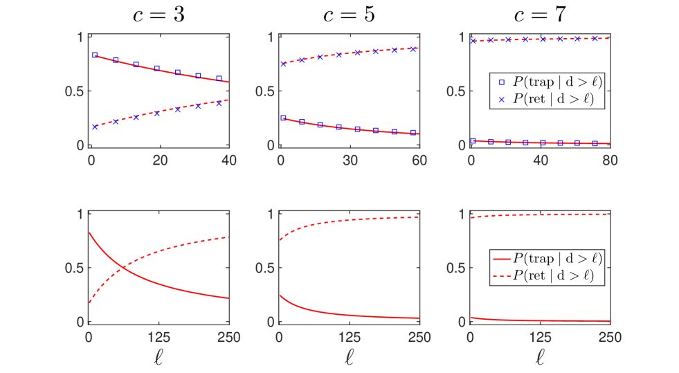
In Fig. 4 we present the probability $p_{\rm trap}$ that an NBW will terminate due to trapping and the probability $p_{\rm ret}$ that it will terminate due to retracing, as a function of the mean degree, $c$, for an ER network of size $N=1000$. As expected, $p_{\rm trap}$ is a decreasing function of $c$ while $p_{\rm ret}$ is an increasing function.

Figure 4: Analytical results for the probabilities $p_{\rm trap}$ (solid line) and $p_{\rm ret}$ (dashed line), that an NBW on an ER network will terminate by trapping in a dead-end node or by retracing of its path, respectively, as a function of the mean degree, $c$. The analytical results, obtained from Eqs. (37) and (38) are found to be in excellent agreement with the results of numerical simulations ($\square$ and $\times$, respectively).

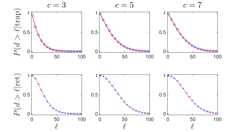
In Fig. 5 we present the probabilities $P(d>\ell|{\rm trap})$ and $P(d>\ell|{\rm ret})$ that an NBW path is of length larger than $\ell$, given that it terminated by trapping or by retracing, respectively. The results are presented for $N=1000$ and $c=3$, $5$ and $7$. The analytical results (solid lines) are found to be in excellent agreement with the numerical simulations (symbols). In both cases, the paths tend to become longer as $c$ is increased. However, for each value of $c$, the paths which terminate due to retracing are typically longer than the paths which terminate due to trapping.

Figure 5: Analytical results for the conditional tail distributions $P(d>\ell|{\rm trap})$ (solid lines) and $P(d>\ell|{\rm ret})$ (dashed lines) of first hitting times vs. $\ell$, for NBWs on an ER network, for paths terminated by trapping (top row) or by retracing (bottom row), respectively. The results are shown for $N=1000$ and $c=3$, $5$ and $7$. The theoretical results for $P(d>\ell|{\rm trap})$ are obtained from Eq. (41), while the theoretical results for $P(d>\ell|{\rm ret})$ are obtained from Eq. (42). In both cases, the theoretical results are found to be in excellent agreement with the numerical simulations ($\square$ and $\times$, respectively).

In Fig. 6 we present the probabilities $P({\rm trap}|d>\ell)$ and $P({\rm ret}|d>\ell)$ that an NBW will terminate due to trapping or retracing, respectively. Results are shown for ER networks of size $N=1000$ and $c=3$, $5$ and $7$. The theoretical results for $P({\rm trap}|d>\ell)$ (solid lines) are obtained from Eq. (47) while the theoretical results for $P({\rm ret}|d>\ell)$ (dashed lines) are obtained from Eq. (48). As expected, it is found that $P({\rm trap}|d>\ell)$ is a monotonically decreasing function of $\ell$ while $P({\rm ret}|d>\ell)$ is monotonically increasing. In the top row these results are compared to the results of numerical simulations (symbols) finding very good agreement. This comparison is done for the range of path lengths which actually appear in the numerical simulations. Longer NBW paths which extend beyond this range become extremely rare, so it is difficult to obtain sufficient numerical data. However, in the bottom row we show the theoretical results for the entire range of path lengths.

Figure 6: The conditional probabilities $P({\rm trap}|d>\ell)$ and $P({\rm ret}|d>\ell)$ that an NBW path will terminate by trapping or by retracing, respectively, given that its length is larger than $\ell$, are presented as a function of $\ell$. Results are shown for an ER networks of size $N=1000$ and $c=3$, $5$ and $7$. The theoretical results for $P({\rm trap}|d>\ell)$ (solid lines) are obtained from Eq. (47) while the theoretical results for $P({\rm ret}|d>\ell)$ (dashed lines) are obtained from Eq. (48). In the top row these results are compared to the results of numerical simulations (symbols) finding very good agreement. This comparison is done for the range of path lengths which actually appear in the numerical simulations and for which good statistics can be obtained. Longer NBW paths which extend beyond this range become extremely rare, so it is difficult to obtain sufficient numerical data. However, in the bottom row we show the theoretical results for a broader range of path lengths. It is found that $P({\rm trap}|d>\ell)$ is a monotonically decreasing function of $\ell$ while $P({\rm ret}|d>\ell)$ is monotonically increasing.

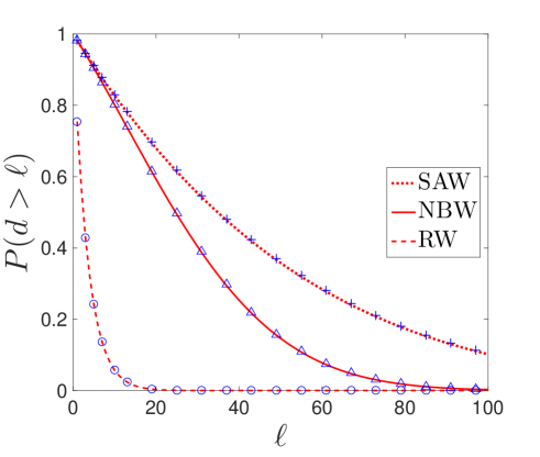
In Fig. 7 we present the tail distribution $P(d>\ell)$ of the first hitting times of the NBW (solid line) on ER networks of size $N=1000$ and $c=3$. It is shown that the paths of the NBW are much longer than those of the simple RW (dashed line), but much shorter than those of the SAW (dotted line) on the same network.

Figure 7: Theoretical results for the tail distribution $P(d>\ell)$ of first hitting times of NBWs (solid line), the tail distribution of first hitting times of RWs (dashed line) and the tail distribution of last hitting times of SAWs (dotted line), on an ER network of size $N=1000$ and $c=4$. The results are in excellent agreement with numerical simulations ($\triangle$, $\circ$ and $+$, respectively). The first hitting times of the NBWs are found to be longer than those of the corresponding RWs, but shorter than the last hitting times of the corresponding SAWs.

7 Generalized non-backtracking random walk models

We will now extend the analysis of the distribution of first hitting times to generalized NBW models with $S>1$. These NBWs keep track of the last $S$ nodes they visited and avoid stepping into them again. In the first $S$ time steps, the generalized NBW behaves like an SAW model. Hence, for $t\leq S$ the conditional probability $P_{\rm trap}(d>t|d>t-1)$ that the NBW will not be trapped at the $t+1$ time step takes the form

$$P_{\rm trap}(d>t|d>t-1)=1-e^{-c(t)},$$ (49)

where $c(t)$ is given by Eq. (4), while the conditional probability

$$P_{\rm ret}(d>t|d>t-1)=1.$$ (50)

The conditional probability $P(d>t|d>t-1)$ can be expressed in the form

$$P(d>t|d>t-1)=P_{\rm trap}(d>t|d>t-1)P_{\rm ret}(d>t|d>t-1)$$ (51)

where $P_{\rm trap}(d>t|d>t-1)$ is the probability that the path will not terminate via the trapping scenario and $P_{\rm ret}(d>t|d>t-1)$ is the probability that it will not terminate via the retracing scenario in the $t+1$ time step.

For $\ell\leq S$ the probability that the NBW path length is longer than $\ell$ is given by

$$P(d>\ell)=P(d>0)\prod_{t=1}^{\ell}P_{\rm trap}(d>t|d>t-1)$$ (52)

or by

$$P\left(d>\ell\right)=\prod_{t=1}^{\ell}\left(1-e^{-c\left(t\right)}\right).$$ (53)

In Ref. [23] it was shown that the tail distribution of path lengths of the SAW model takes the form

$$P_{\rm trap}(d>\ell)\simeq\exp\left\{\frac{N-1}{c}\left[{\rm Li}_{2}\left(e^{-c+\frac{c}{2(N-1)}}\right)-{\rm Li}_{2}\left(e^{-c+\frac{(2\ell+1)c}{2(N-1)}}\right)\right]\right\}.$$ (54)

where ${\rm Li}_{n}(x)$ is the Polylogarithm function [45]. For large networks ($N\gg 1$) one can approximate Eq. (54) by

$$P_{\rm trap}(d>\ell)\simeq\exp\left[-\eta\left(e^{b\ell}-1\right)\right],$$ (55)

which is a discrete form of the Gompertz distribution [29, 30, 31, 32], where

$$b=\frac{c}{N}$$ (56)

is the scale parameter and

$$\eta=\frac{N}{c}e^{-c}$$ (57)

is the shape parameter.

Starting at time step $t=S+1$ the NBW may hop into nodes which were already visited before at times $t^{\prime}=0,1,\dots,t-S-1$, thus causing termination of the path through the retracing mechanism. The step in which the NBW hops into a previously visited node is not counted as a part of the RW path. This means that the path length of an NBW which pursued $\ell$ steps and was terminated in the $\ell+1$ step, is $d=\ell$. The path includes $\ell+1$ nodes, since the initial node is counted as a part of the path.

In case that the NBW has already pursued $t>S$ steps without visiting any node more than once, the path length is guaranteed to be $d>t-1$. At this point, the probability that the path will not terminate by trapping in the $t+1$ step is denoted by the conditional probability $P_{\rm trap}(d>t|d>t-1)$. We will now evaluate this probability for $t>S$. The probability that the node entered by the NBW at time $t$ does not have any other neighbor except for those nodes visited in the last $S$ time steps is given by $e^{-c(S-1)}$. This conditional probability is thus given by

$$P_{\rm trap}(d>t|d>t-1)=1-e^{-c(S-1)},$$ (58)

where $c(S-1)$ is given by Eq. (4). For $t>S$ there are $N-S-1$ nodes, which may be connected to the current node with probability $p$. Having eliminated the possibility of trapping at the $t+1$ time step, guarantees that at least one of these nodes is actually connected to the current node. Each one of the remaining $N-S-2$ nodes is connected to the current node with probability $p$. Thus, the expectation value of the number of neighbors of the current node to which the NBW may hop is $(N-S-2)p+1$. Due to the local tree-like structure of ER networks, it is extremely unlikely that the one node which is guaranteed to be connected to the current node has already been visited. This is due to the fact that the path from such earlier visit all the way to the current node is essentially a loop. Therefore, we conclude that this adjacent node has not been visited yet. Since the number of yet unvisited nodes is $N-t-1$, the current node is expected to have $(N-t-2)p+1$ neighbors which have not yet been visited. As a result, the probability that in the $t+1$ time step the NBW will hop into one of the yet-unvisited nodes is given by

$$P_{\rm ret}(d>t|d>t-1)=\frac{(N-t-2)p+1}{(N-S-2)p+1}.$$ (59)

Using the fact that $c=(N-1)p$ and $c(t)=(N-t-1)p$ we obtain

$$P_{\rm ret}(d>t|d>t-1)=\frac{c(t)-p+1}{c-(S+1)p+1}.$$ (60)

Summarizing the results so far, we obtain that for $t\leq S$ the conditional probability $P(d>t|d>t-1)$ is given by Eq. (51), while for $t>S$

$$P(d>t|d>t-1)=\left[\frac{c(t)-p+1}{c-(S+1)p+1}\right]\left[1-e^{-c(S-1)}\right].$$ (61)

In Fig. 8 we present the conditional probability $P(d>t|d>t-1)$ vs. $t$ for the generalized NBW model with $S=25$, $50$ and $100$ on an ER network of size $N=1000$ and mean degree $c=3$, $4$ and $10$. The analytical results (solid lines) obtained from Eqs. (49) and (61) are found to be in good agreement with numerical simulations (symbols), confirming the validity of these equations. Note that the numerical results become more noisy as $t$ increases, due to diminishing statistics, and eventually terminate. This is particularly apparent for the smaller values of $c$.

Figure 8: The conditional probability $P(d>\ell|d>\ell-1)$ vs. $\ell$, obtained from Eqs. (49) and (61) (solid lines) and from numerical simulations (symbols) of generalized NBWs with $S=25$ (left), $S=50$ (center) and $S=100$ (right), on ER networks of size $N=1000$ and mean degrees $c=3$, $4$ and $10$ (squares, triangles and circles, respectively). The analytical and numerical results are found to be in good agreement.

In Appendix B we calculate the probabilities $P_{\rm ret}(d>\ell)$ and $P_{\rm trap}(d>\ell)$ and obtain

$${P\left(d>\ell\right)=\left\{\begin{array}[]{ll}\exp\left[-\eta\left(e^{b\ell}-1\right)\right]&\ell\leq S\\ \exp\left[-\eta\left(e^{bS}-1\right)\right]\exp\left[-\frac{\ell_{S}(\ell_{S}-1)}{2\alpha^{2}}-\beta_{S}\ell_{S}\right]&\ell\geq S+1,\end{array}\right.}$$ (62)

where

$$\beta_{S}=-\ln\left[1-e^{-\left(1-\frac{S-1}{N-1}\right)c}\right],$$ (63)

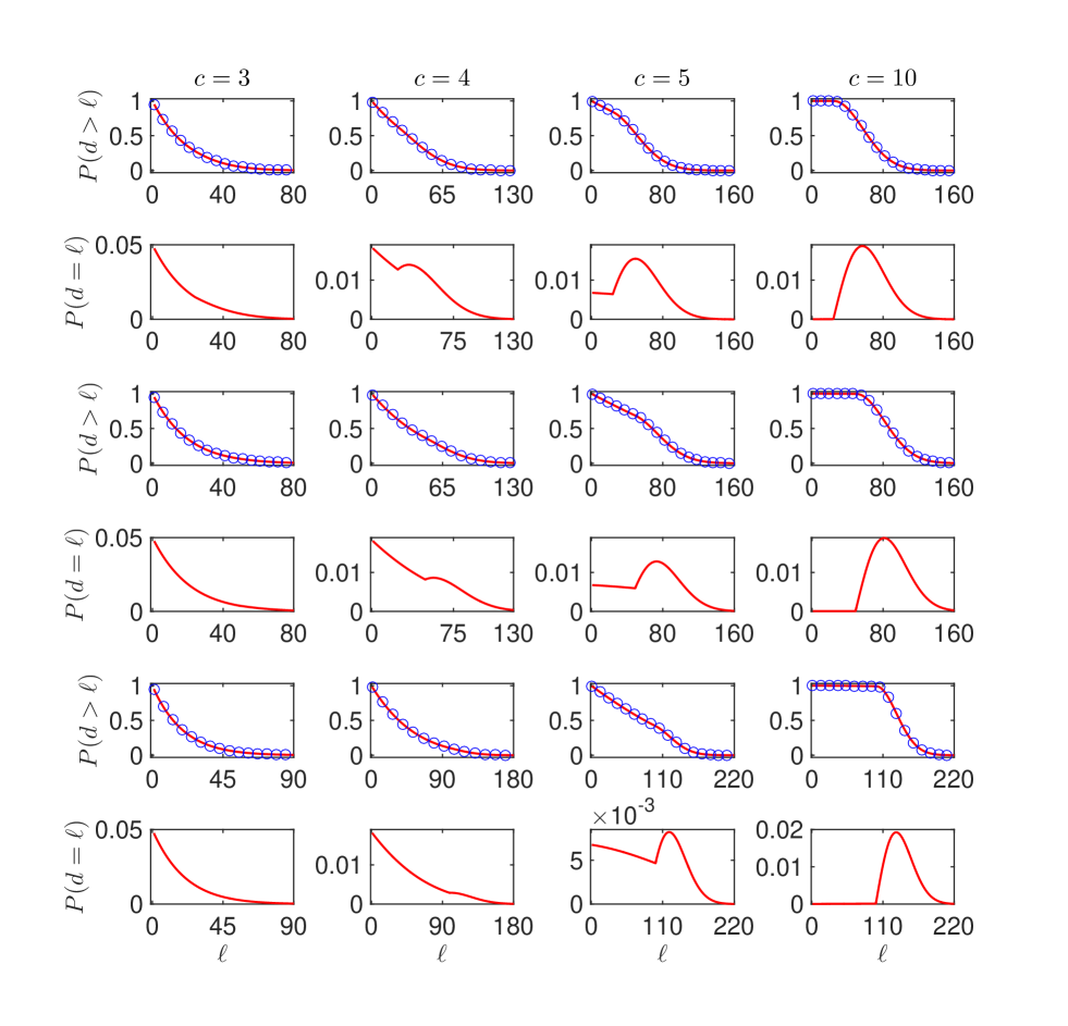
and $\ell_{S}=\ell-(S-1)$. In Fig. 9 we present the tail distributions of first hitting times $P(d>\ell)$ (top rows) vs. $\ell$ for generalized NBWs with $S=25$, $50$ and $100$ on ER networks of size $N=1000$ and mean degrees $c=3$, $4$, $5$ and $10$. The theoretical results (solid lines) were obtained from Eq. (62). They are found to be in excellent agreement with the numerical simulations (symbols). The theoretical results for the probability distribution functions are presented in the bottom rows.

Figure 9: The tail distributions, $P(d>\ell)$, of first hitting times and the corresponding probability density functions, $P(d=\ell)$, vs. $\ell$, of generalized NBWs with $S=25$ (rows 1 and 2), $S=50$ (rows 3 and 4) and $S=100$ (rows 5 and 6) on ER networks of size $N=1000$ and $c=3$, $4$, $5$ and $10$. The theoretical results, obtained from Eqs. (62) (solid lines), are found to be in excellent agreement with the results obtained from numerical simulations (circles). The agreement with the numerical results is already established for the tail distributions and therefore the numerical data is not shown for the probability density functions.

In order to obtain an expression for the mean distance, $\ell_{\rm mean}$, we use the tail-sum formula presented in Eq. (27) for $n=1$. Separating the sum into two parts, one for $\ell\leq S$ and the other for $\ell>S$, we obtain

$$\ell_{\rm mean}=\sum_{\ell=0}^{S}P_{\rm trap}\left(d>\ell\right)+\sum_{\ell=S+1}^{N-2}P\left(d>\ell\right).$$ (64)

In Appendix C we evaluate these sums and obtain

$$\ell_{\rm mean} \simeq 1+\frac{e^{\eta}}{b}\left[{\rm Ei}\left(-\eta e^{b(S+{1}/{2})}\right)-{\rm Ei}\left(-\eta e^{\frac{b}{2}}\right)\right]$$ (65)

$$+ \sqrt{\frac{\pi}{2}}\alpha\exp\left[\frac{(\alpha^{2}\beta_{S}-1)\beta_{S}}{2}-\eta\left(e^{bS}-1\right)\right]$$

$$\times \left[{\rm erf}\left(\frac{\alpha^{2}\beta_{S}+(N-S)-2}{\sqrt{2}\alpha}\right)-{\rm erf}\left(\frac{\alpha\beta_{S}}{\sqrt{2}}\right)\right],$$

where the shape parameter $\eta$ is given by Eq. (57), the scale parameter $b$ is given by Eq. (56), the parameter $\beta_{S}$ is given by Eq. (63) and $\alpha$ is given by (17).

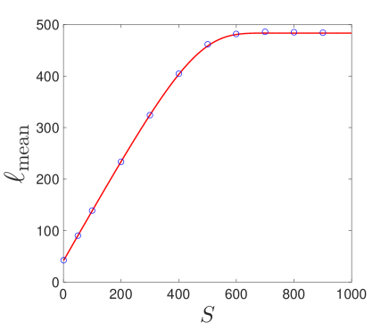
In Fig. 10 we present the mean of the distribution of first hitting times, $\ell_{mean}$, as a function of the mean degree, $c$, of generalized NBWs with $S=25$ (a), $S=50$ (b) and $S=100$ (c) on ER networks of size $N=1000$. The analytical results (solid line), obtained from Eq. (65) are in excellent agreement with numerical simulations (circles). It is shown that $\ell_{mean}$ increases sharply as a function of $c$ and quickly saturates. As $S$ is increased, the saturation level of $\ell_{mean}$ increases.

Figure 10: The mean of the distribution of first hitting times, $\ell_{mean}$, as a function of the mean degree, $c$, of generalized NBWs with $S=25$ ($\circ$), $S=50$ ($\square$) and $S=100$ ($\times$) on ER networks of size $N=1000$. The analytical results (solid lines), obtained from Eq. (65) are in excellent agreement with numerical simulations (symbols).

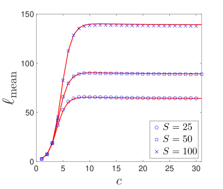
In Fig. 11 we present the mean of the distribution of first hitting times, $\ell_{mean}$, as a function of $S$ for generalized NBWs on an ER network of size $N=1000$ and $c=10$ . The analytical results (solid line), obtained from Eq. (65) are in excellent agreement with numerical simulations (circles).

Figure 11: The mean of the distribution of first hitting times, $\ell_{mean}$, as a function of $S$ for generalized NBWs on an ER network of size $N=1000$ and $c=10$ . The analytical results (solid line), obtained from Eq. (65), are in excellent agreement with numerical simulations (circles).

The paths of generalized NBWs may terminate either by the trapping scenario or by the retracing scenario. Therefore, the tail distribution $P(d>\ell)$ can be decomposed into two distributions, each accounting for the paths terminated by one of the two scenarios. First, we calculate the probabilities, $p_{\rm trap}$ and $p_{\rm ret}$, that a generalized NBW path will terminate by the trapping scenario or by the retracing scenario, respectively. The probability of termination by trapping, $p_{\rm trap}$ is given by

$$p_{\rm trap}=p_{\rm trap}[d\leq S]+p_{\rm trap}[d\geq S+1],$$ (66)

where $p_{\rm trap}[d\leq S]$ is the probability that a generalized NBW path will terminate by trapping during the first $S$ time steps, while $p_{\rm trap}[d>S]$ is the probability that it will terminate by trapping after more than $S$ steps. These probabilities are given by

$$p_{\rm trap}[d\leq S]=\sum_{\ell=1}^{S}P_{\rm trap}(d>\ell-1)[1-P_{\rm trap}(d>\ell|d>\ell-1)],$$ (67)

and

$$p_{\rm trap}[d\geq S+1]=\sum_{\ell=S+1}^{N-2}P(d>\ell-1|d\geq S+1)[1-P_{\rm trap}(d>\ell|d>\ell-1)].$$ (68)

Summing up the terms on the right hand side of Eq. (67), it can be written in the form

$$p_{\rm trap}[d\leq S]=P_{\rm trap}(d>0)-P_{\rm trap}(d>S).$$ (69)

One can evaluate the sum on the right hand side of Eq. (67) by converting it to an integral of the form

$$p_{\rm trap}[d\leq S]=\int_{1/2}^{S+1/2}b\eta\exp\left[-\eta\left(e^{b(\ell-1)}-1\right)+\frac{c}{N}\ell\right]d\ell.$$ (70)

Solving the integral we obtain

$$p_{\rm trap}[d\leq S]=\exp\left[\eta\left(1-e^{\frac{-b}{2}}\right)\right]-\exp\left[\eta\left(1-e^{b\left(S-\frac{1}{2}\right)}\right)\right]$$ (71)

Converting the sum on the right hand side of Eq. (68) to an integral and performing the integration we obtain

$$p_{\rm trap}[d\geq S+1] = \left\{1+\sqrt{\frac{\pi}{2}}\alpha e^{\frac{(\alpha^{2}\beta_{S}-1)\beta_{S}}{2}}\left[{\rm erf}\left(\frac{\alpha^{2}\beta_{S}+N-S-2}{\sqrt{2}\alpha}\right)\right.\right.$$ (72)

$$- \left.\left.{\rm erf}\left(\frac{\alpha\beta_{S}}{\sqrt{2}}\right)\right]\right\}e^{-c\left(S-1\right)}.$$

Combining the results of Eqs. (71) and (72) we find that

$$p_{\rm trap}=\exp\left[\eta\left(1-e^{\frac{-b}{2}}\right)\right]-\exp\left[\eta\left(1-e^{b\left(S-\frac{1}{2}\right)}\right)\right]$$

$$+\left\{1+\sqrt{\frac{\pi}{2}}\alpha e^{\frac{(\alpha^{2}\beta_{S}-1)\beta_{S}}{2}}\left[{\rm erf}\left(\frac{\alpha^{2}\beta_{S}+N-S-2}{\sqrt{2}\alpha}\right)-{\rm erf}\left(\frac{\alpha\beta_{S}}{\sqrt{2}}\right)\right]\right\}e^{-c\left(S-1\right)}.$$ (73)

The probability of termination by the retracing scenario is obtained from $p_{\rm ret}=1-p_{\rm trap}$, or

$$p_{\rm ret}=1-\exp\left[\eta\left(1-e^{\frac{-b}{2}}\right)\right]+\exp\left[\eta\left(1-e^{b\left(S-\frac{1}{2}\right)}\right)\right]$$

$$-\left\{1+\sqrt{\frac{\pi}{2}}\alpha e^{\frac{(\alpha^{2}\beta_{S}-1)\beta_{S}}{2}}\left[{\rm erf}\left(\frac{\alpha^{2}\beta_{S}+N-S-2}{\sqrt{2}\alpha}\right)-{\rm erf}\left(\frac{\alpha\beta_{S}}{\sqrt{2}}\right)\right]\right\}e^{-c\left(S-1\right)}.$$ (74)

It turns out that for values of $c$ which are not too small, the approximation involves in converting the sum of Eq. (68) to an integral is very good and Eqs. (73) and (74) provide accurate results for $p_{\rm trap}$ and $p_{\rm ret}$, respectively. However, for small values of $c$, more accurate results are obtained by using the recursion equations directly to evaluate $p_{\rm trap}[d\leq S]$ from Eq. (69).

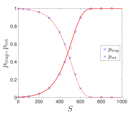
In Fig. 12 we present the probabilities $p_{\rm trap}$ and $p_{\rm ret}$ that generalized NBWs with $S=25$, $50$ and $100$ on an ER network will terminate via retracing of its path, or by being trapped in a dead-end node, respectively, as a function of the mean degree, $c$. The theoretical results, obtained from Eqs. (73) and (74) are found to be in excellent agreement with the results of numerical simulations (symbols).

Figure 12: Analytical results for the probabilities $p_{\rm trap}$ (solid lines) and $p_{\rm ret}$ (dashed lines) that generalized NBWs with $S=25$, $50$ and $100$ on an ER network will terminate by retracing their paths, or by being trapped in a dead-end node, respectively, as a function of the mean degree, $c$. The theoretical results, obtained from Eqs. (73) and (74) are found to be in excellent agreement with the results of numerical simulations (symbols).

In Fig. 13 we present the probabilities $p_{\rm trap}$ and $p_{\rm ret}$ that a generalized NBW path will terminate by trapping or by retracing, respectively, as a function of the parameter $S$ on an ER network of size $N=1000$ and $c=10$. The theoretical results, obtained from Eqs. (73) and (74) are found to be in excellent agreement with the results of numerical simulations (symbols).

Figure 13: Analytical results for the probabilities $p_{\rm trap}$ (solid line) and $p_{\rm ret}$ (dashed line) that a generalized NBW will terminate by trapping in a dead-end node or by retracing of its path, respectively, as a function of the parameter $S$ on an ER network of size $N=1000$ and $c=10$. The theoretical results for $p_{\rm trap}$ (solid line), obtained from Eq. (73), and for $p_{\rm ret}$ (dashed line), obtained from Eq. (74), are found to be in excellent agreement with the results of numerical simulations (symbols).

We will now calculate the conditional tail distribution of the path lengths of generalized NBW paths. The probability that an NBW path length will be larger than $\ell$, given that it terminated by trapping is given by $P\left(d>\ell|{\rm trap}\right)$, while the probability that it will be larger than $\ell$ given that it terminated by retracing is given by $P\left(d>\ell|{\rm ret}\right)$. The probability $P\left(d>\ell|{\rm trap}\right)$ is given by

$$P\left(d>\ell|{\rm trap}\right)=\frac{1}{p_{\rm trap}}\sum_{t=\ell+1}^{N-2}P\left(d>t-1\right)\left[1-P_{\rm trap}\left(d>t|d>t-1\right)\right].$$ (75)

It can be expressed in the form

$${P\left(d>\ell|{\rm trap}\right)=\left\{\begin{array}[]{ll}\sum\limits_{t=\ell+1}^{S}e^{-c\left(t\right)}\frac{P\left(d>t-1\right)}{p_{\rm trap}}+{e^{-c\left(S-1\right)}}\sum\limits_{t=S+1}^{N-1}\frac{P\left(d>t-1\right)}{p_{\rm trap}}&\ell\leq S\\ {e^{-c\left(S-1\right)}}\sum\limits_{t=\ell}^{N-1}\frac{P\left(d>t-1\right)}{p_{\rm trap}}&\ell\geq S+1\end{array}\right.}$$ (76)

The conditional tail distribution $P\left(d>\ell|{\rm ret}\right)$ can be written in the form

$$P\left(d>\ell|{\rm ret}\right) = \frac{1}{p_{\rm ret}}\sum\limits_{t=\ell}^{N-2}P\left(d>t-1\right)P_{\rm trap}\left(d>t|d>t-1\right)$$ (77)

$$\times \left[1-P_{\rm ret}\left(d>t|d>t-1\right)\right].$$

Thus, we find that

$${P\left(d>\ell|{\rm ret}\right)=\left\{\begin{array}[]{ll}1&\ell\leq S\\ \frac{1-e^{-c\left(S-1\right)}}{p_{\rm ret}}\sum\limits_{t=\ell}^{N-2}P\left(d>t-1\right)\left[\frac{c-c\left(t\right)-Sp}{c-(S+1)p+1}\right]&\ell\geq S+1\end{array}\right.}$$ (78)

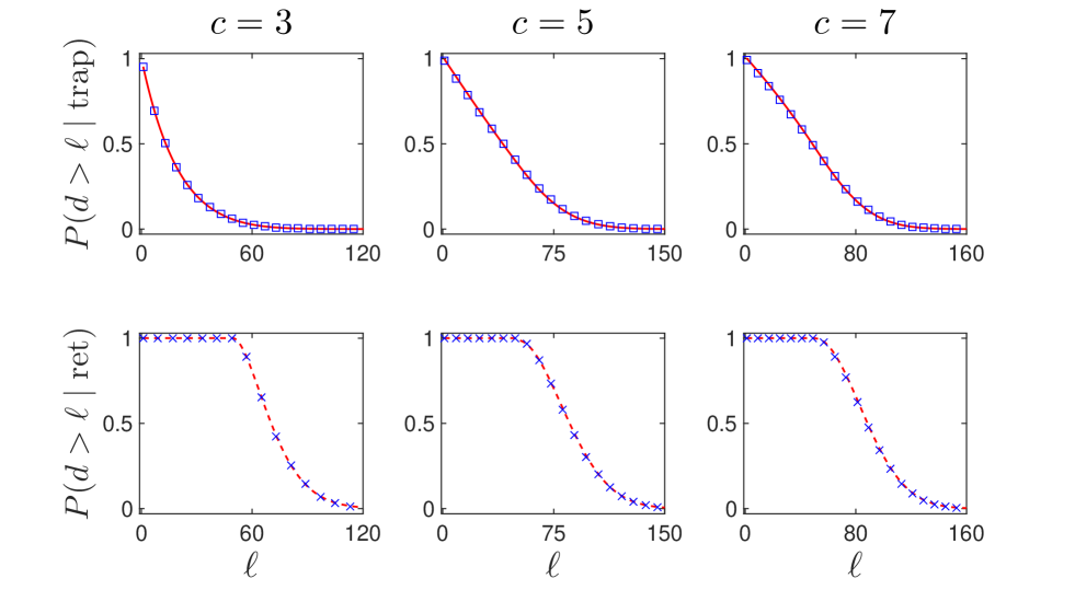
In Fig. 14 we present the conditional tail distributions $P(d>\ell|{\rm trap})$ and $P(d>\ell|{\rm ret})$ of first hitting times vs. $\ell$, for NBWs on an ER network of size $N=1000$ and $c=3$, $5$ and $7$. The theoretical results, obtained from Eqs. (76) and (78) are found to be in excellent agreement with the numerical simulations.

Figure 14: The conditional tail distributions $P(d>\ell|{\rm trap})$ and $P(d>\ell|{\rm ret})$ of first hitting times vs. $\ell$, of generalized NBWs with $S=50$, for paths terminated by trapping (top row) or by retracing (bottom row), respectively. The results are shown for ER networks of size $N=1000$ and $c=3$, $5$ and $7$. The theoretical results for $P(d>\ell|{\rm trap})$ are obtained from Eq. (76), while the theoretical results for $P(d>\ell|{\rm ret})$ are obtained from Eq. (78). In both cases, the theoretical results (solid and dashed lines lines, respectively) are found to be in excellent agreement with the numerical simulations (symbols).

Finally, we use Bayes’ theorem to obtain the conditional distributions:

$${P\left({\rm trap}|d>\ell\right)=\left\{\begin{array}[]{ll}\sum\limits_{t=\ell+1}^{S-1}e^{-c\left(t\right)}\frac{P\left(d>t-1\right)}{P\left(d>\ell\right)}+e^{-c(S-1)}\sum\limits_{t=S}^{N}\frac{P\left(d>t-1\right)}{P\left(d>\ell\right)}&\ell\leq S\\ e^{-c\left(S-1\right)}\sum\limits_{t=\ell+1}^{N}P\left(d>t-1\right)&\ell\geq S+1\end{array}\right.}$$ (79)

and

$${P\left({\rm ret}|d>\ell\right)=\left\{\begin{array}[]{ll}\frac{\left[1-e^{-c\left(S-1\right)}\right]}{P\left(d>\ell\right)}\sum\limits_{t=S}^{N}\left[\frac{c-c\left(t\right)-Sp}{c-(S+1)p+1}\right]{P\left(d>t-1\right)}&\ell\leq S\\ \frac{\left[1-e^{-c\left(S-1\right)}\right]}{P\left(d>\ell\right)}\sum\limits_{t=\ell}^{N-2}\left[\frac{c-c\left(t\right)-Sp}{c-(S+1)p+1}\right]{P\left(d>t-1\right)}&\ell\geq S+1\end{array}\right.}$$ (80)

In Fig. 15 we present the conditional probabilities $P({\rm trap}|d>\ell)$ and $P({\rm ret}|d>\ell)$ that an NBW path will terminate by trapping or by retracing, respectively, given that its length is larger than $\ell$, as a function of $\ell$. Results are shown for ER networks of size $N=1000$ and $c=3$, $5$ and $7$. The theoretical results, obtained from Eqs. (79) and (80) are found to be in excellent agreement with the numerical simulations. This comparison is done for the range of path lengths which actually appear in the numerical simulations and for which good statistics can be obtained. Longer RW paths which extend beyond this range become extremely rare, so it is difficult to obtain sufficient numerical data. However, in the bottom row we show the theoretical results for the entire range of path lengths. In fact, such long paths can be sampled using the pruned enriched Rosenbluth method, which was successfully used in the context of SAWs in polymer physics [46]. In this method one samples long non-overlapping paths, keeping track of their weights, to obtain an unbiased sampling in the ensemble of all paths.

Figure 15: The conditional probabilities $P({\rm trap}|d>\ell)$ and $P({\rm ret}|d>\ell)$ that a path of a generalized NBW with $S=50$ will terminate by trapping or by retracing, respectively, given that its length is larger than $\ell$, are presented as a function of $\ell$. Results are shown for ER networks of size $N=1000$ and $c=3$, $5$ and $7$. The theoretical results for $P({\rm trap}|d>\ell)$ (solid lines) are obtained from Eq. (79) while the theoretical results for $P({\rm ret}|d>\ell)$ (dashed lines) are obtained from Eq. (80). The theoretical results are compared to the results of numerical simulations (symbols) finding excellent agreement. It is found that $P({\rm trap}|d>\ell)$ is a monotonically decreasing function of $\ell$ while $P({\rm ret}|d>\ell)$ is monotonically increasing.

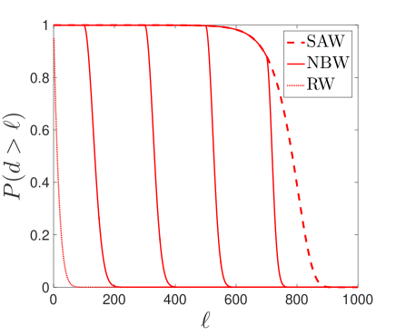
In Fig. 16 we present theoretical results for the tail distributions $P(d>\ell)$ of first hitting times of generalized NBWs with $S=100$, $300$, $500$ and $700$ (solid lines, left to right), in comparison with the tail distribution of first hitting times of RWs (dashed line) and the tail distribution of last hitting times of SAWs (dotted line), on an ER network of size $N=1000$ and $c=20$. As $S$ is increased, the form of the tail distribution exhibits a crossover from the RW towards the SAW.

Figure 16: Theoretical results for the tail distributions $P(d>\ell)$ of first hitting times of generalized NBWs with $S=100$, $300$, $500$ and $700$ (solid lines, left to right), in comparison with the tail distribution of first hitting times of RWs (dotted line) and the tail distribution of last hitting times of SAWs (dashed line), on an ER network of size $N=1000$ and $c=20$. As $S$ is increased, the tail distribution of first hitting times of the generalized NBWs exhibits a crossover from the behavior of a RW towards the behavior of an SAW.

8 Summary and Discussion

NBWs provide useful insight on the dynamics of objects which exhibit random motion on networks such as web crawlers and foragers. Starting from a random initial node, these walkers hop randomly between adjacent nodes without backtracking, namely without hopping back into the previous node. The NBW path terminates when it steps into a node which they already visited before (retracing scenario) or when it becomes trapped in a dead-end node from which it cannot exit (trapping scenario). The number of steps taken from the initial node up to the termination of the path is called the first hitting time. We obtained analytical results for the distribution of first hitting times, $P(d=\ell)$, of NBWs on ER networks and for its mean, median and standard deviation. We calculated the probabilities, $p_{\rm trap}$ and $p_{\rm ret}$, that an NBW path starting at a random node will terminate by trapping or by retracing, respectively. We also obtained analytical expressions for the conditional distributions of path lengths, $P(d=\ell|{\rm trap})$ and $P(d=\ell|{\rm ret})$ for the paths which terminate by backtracking and by retracing, respectively. Finally, we calculated the conditional probabilities $P({\rm trap}|d=\ell)$ and $P({\rm ret}|d=\ell)$ that a path which terminates after $d=\ell$ steps is terminated by trapping or by retracing, respectively. It was found that the two termination mechanisms exhibit very different behavior. The trapping probability sets in starting from the second step and is constant throughout the path. As a result, this mechanism alone would produce a geometric distribution of path lengths. The retracing mechanisms sets in starting from the third step and its rate increases linearly in time. The balance between the two termination mechanisms depends on the mean degree of the network. In the limit of sparse networks, the trapping mechanism is dominant and most paths terminate long before the retracing mechanism becomes relevant. In the case of dense networks, the trapping probability is low and most paths terminate by the retracing mechanism.

Comparing the NBW model studied here to the RW model studied in Ref. [35], we find that the probability of termination by retracing at time $t$, given by

$$P_{\rm ret}(d=t|d>t-1)=1-P_{\rm ret}(d>t|d>t-1)=\frac{c-c(t)}{c+1},$$ (81)

is identical in the two models. It can be expressed in the form

$$P_{\rm ret}(d=t|d>t-1)=\left(\frac{c}{c+1}\right)\left(\frac{t}{N-1}\right).$$ (82)

The difference between the distributions of first hitting times in the two models is due to the different behaviors of the backtracking mechanism in the RW model and the trapping mechanism in the NBW model. While the probabilities of both backtracking and trapping do not depend on time, they depend differently on the parameter $c$. The backtracking probability is given by [35]

$$P_{\rm backtrack}(d=t|d>t-1)=1-P_{\rm backtrack}(d>t|d>t-1)=\frac{1-e^{-c}}{c},$$ (83)

while the trapping probability is given by

$$P_{\rm trap}(d=t|d>t-1)=1-P_{\rm trap}(d>t|d>t-1)=e^{-c}.$$ (84)

This means that the backtracking probability essentially decreases as $1/c$ while the trapping probability decreases exponentially. Therefore, the trapping mechanism is much less likely to occur and the NBW paths are are much longer than the corresponding RW paths.

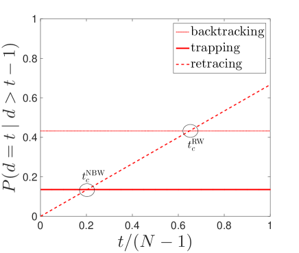
In Fig. 17 we present the termination probabilities by backtracking (of RWs), by trapping (of NBWs) and by retracing (both RWs and NBWs) as a function of time, on an ER network of size $N=1000$ and $c=2$. While the backtracking and trapping probabilities do not depend on time, the retracing probability increases linearly with time. The RW model exhibits a crossover time, $t_{c}^{\rm RW}$, at which the retracing probability exceeds the backtracking probability. This crossover time is given by

$$\frac{t_{c}^{\rm RW}}{N-1}=\left(\frac{c+1}{c}\right)\left(\frac{1-e^{-c}}{c}\right)$$ (85)

Similarly, the NBW model exhibits a crossover time, $t_{c}^{\rm NBW}$, given by

$$\frac{t_{c}^{\rm NBW}}{N-1}=\left(\frac{c+1}{c}\right)e^{-c},$$ (86)

at which the retracing probability exceeds the trapping probability.

Figure 17: The probability $P_{\rm backtrack}(d=t|d>t-1)$ that a RW will terminate by backtracking at time $t$ (dotted line), the probability $P_{\rm trap}(d=t|d>t-1)$ that an NBW will terminate by trapping at time $t$ (solid line) and the probability $P_{\rm ret}(d=t|d>t-1)$ that either a RW or an NBW will terminate by retracing at time $t$ (dashed line), vs. the normalized time, $t/(N-1)$, for an ER network of $N=1000$ nodes and $c=2$. While the backtracking and trapping probabilities do not depend on time, the retracing probability increases linearly with time. Since the backtracking probability is larger than the trapping probability, the crossover time $t_{c}^{\rm RW}$ in which the retracing probability exceeds the backtracking probability is larger than the crossover time $t_{c}^{\rm NBW}$ in which the retracing probability exceeds the trapping probability.

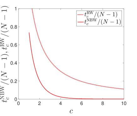
In Fig. 18 we present the normalized crossover times $t_{c}^{\rm RW}/(N-1)$ and $t_{c}^{\rm NBW}/(N-1)$ of RWs and NBWs, respectively, as a function of the mean degree, $c$, on an ER network of size $N=1000$. While both times are decreasing functions of $c$, the crossover time of the RW is larger than the crossover time of the NBW for all values of $c>1$.

Figure 18: The normalized crossover time, $t_{c}^{\rm RW}/(N-1)$, in which the retracing probability exceeds the backtracking probability of the RW (dashed line) and the normalized crossover time $t_{c}^{\rm NBW}/(N-1)$ (solid line) at which the retracing probability exceeds the trapping probability of the NBW, as a function of $c$ for an ER network of size $N=1000$. Both crossover times decrease as $c$ is increased, while $t_{c}^{\rm RW}>t_{c}^{\rm NBW}$ for all values of $c$.

We also considered generalized NBWs which keep track of the last $S$ visited nodes and avoid hopping into them. The parameter, $S$, may take values in the range $1\leq S\leq N-1$. The case of $S=1$ is the NBW model, in which backtracking into the previous node is not allowed. The paths of NBWs may terminate either by hopping into nodes already visited at earlier times (retracing) or by trapping in a leaf node of degree $k=1$ from which they cannot exit. Generalized NBW models, with $S>1$, avoid hopping into any of the nodes visited at times $t=1$, $t-2$, $\dots$, $t-S$. The paths of generalized NBWs may terminate either by retracing or by trapping in a node which is surrounded by the tail of $S$ nodes which they cannot enter. Thus, unlike the NBW which may be trapped only at a node of degree $k=1$, the generalized NBW may be trapped at nodes of degrees $k\leq S$. The case of $S=N-1$ coincides with the SAW model. During the first $S+1$ time steps, the generalized NBW behaves like an SAW and may terminate only by trapping. Starting at the $S+2$ step, the retracing mechanism is activated and from that point on its weight increases linearly with time. Thus, the probability of termination by trapping $p_{\rm trap}$ is an increasing function of $S$, while the probability of termination by retracing $p_{\rm ret}$ is a decreasing function of $S$. Overall, the mean path length of the generalized NBW increases as $S$ is increased.

The analysis presented in this paper provides useful insight on the broad issue of life-time distributions such as the distribution of life expectancies of humans and animals and the distribution of service lives of machines [47, 48]. In particular, the RW, NBW and SAW provide well defined termination mechanisms for which the distributions of termination times can be calculated analytically. In case of the SAW, the termination rate increases exponentially with time, giving rise to a distribution of termination times which follows the Gompertz distribution. In case of the RW and NBW, the termination rate consists of a constant term and a linearly increasing term, resulting in a distribution of termination times which follows a combination of an exponential distribution and a Rayleigh distribution. The termination rate of the generalized NBW resembles an SAW in the first $S$ steps and an NBW afterwards. Interestingly, the life expectancies of humans can be described by the Gompertz distribution [29, 30, 31, 32], while the service lives of machines can be fitted to a Weibull distribution, of which the Rayleigh distribution is a special case [49]. In general, the distribution of human life expectancies and the distribution of machine service lives are determined by a combination of different causes of death or failure mechanisms. To understand the interplay between these different scenarios one needs to be able to isolate the contribution of each of of them and examine how it varies with age. In the analysis of the termination scenarios of NBW paths we develop an approach which enables us to disentangle the contribution of the trapping and retracing mechanisms. This type of analysis is likely to be useful in many other contexts in which several failure mechanisms coexist.

Appendix A Calculation of $P(d>\ell)$ for the NBW model

To obtain a closed form expression for the tail distribution, $P(d>\ell)$, we take the natural logarithm on both sides of Eq. (13). This leads to

$$\ln\left[P\left(d>\ell\right)\right]=\ln\left[P_{\rm ret}\left(d>\ell\right)\right]+\ln\left[P_{\rm trap}\left(d>\ell\right)\right].$$ (87)

Below we analyze separately each one of the two terms on the right hand side of Eq. (87). The calculation of the tail distribution $P_{\rm trap}(d>\ell)$ is simplified by the fact that $P_{\rm trap}(d>t|d>t-1)$ does not depend on $t$. As a result, Eq. (14) can be written in the form

$$P_{\rm trap}(d>\ell)=\left(1-e^{-c}\right)^{\ell},$$ (88)

or in the form

$$P_{\rm trap}(d>\ell)=e^{-\beta\ell},$$ (89)

where

$$\beta=-\ln\left(1-e^{-c}\right).$$ (90)

The termination by the trapping scenario can be considered as a Poisson process, in which the termination probability is fixed and depends only on the mean degree of the network.

Taking the logarithm of $P_{\rm ret}(d>\ell)$, as expressed in Eq. (15), we obtain

$$\ln\left[P_{\rm ret}(d>\ell)\right]=\sum_{t=2}^{\ell}\ln\left[\frac{c(t)-p+1}{c-2p+1}\right].$$ (91)

Replacing the sum by an integral we obtain

$$\ln P_{\rm ret}(d>\ell)\simeq\int_{3/2}^{\ell+1/2}\ln\left[\frac{c\left(t\right)-p+1}{c-2p+1}\right]dt.$$ (92)

Plugging in the expression for $c(t)$ from Eq. (4) and rearranging terms in the integrand we obtain

$$\ln P_{\rm ret}(d>\ell)\simeq\int_{3/2}^{\ell+1/2}\ln\left[1-\frac{(t-1)c}{\left(N-1\right)\left(c-2p+1\right)}\right]dt.$$ (93)

For sufficiently large networks one can replace $N-1$ by $N$ and $c+1-2p$ by $c+1$. Solving the integral we obtain

$$\ln[P_{\rm ret}(d>\ell)] \simeq \left(\ell-\frac{1}{2}-\alpha^{2}\right)\ln\left(1-\frac{\ell-1/2}{\alpha^{2}}\right)-(\ell-1)$$ (94)

$$+ \left(\alpha^{2}-\frac{1}{2}\right)\ln\left(1-\frac{1}{2\alpha^{2}}\right),$$

where

$$\alpha=\sqrt{\frac{N\left(c+1\right)}{c}}.$$ (95)

In the approximation of the sum of Eq. (91) by the integral of Eq. (92) we have used the formulation of the middle Riemann sum. Since the function $\ln[P_{r}(d>\ell)]$ is a monotonically decreasing function, the value of the integral is over-estimated by the left Riemann sum, $L_{\alpha}(\ell)$, and under-estimated by the right Riemann sum, $R_{\alpha}(\ell)$. The error involved in this approximation is thus bounded by the difference $\Delta_{\alpha}(\ell)=L_{\alpha}(\ell)-R_{\alpha}(\ell)$, which satisfies $\Delta_{\alpha}(\ell)<\ln(1-\ell/\alpha^{2})$. Thus, the relative error in $P(d>\ell)$ due to the approximation of the sum by an integral is bounded by $\eta_{\rm SI}=\ell/\alpha^{2}$, which scales like $\ell/N$. Comparing the values obtained from the sum and the integral over a broad range of parameters, we find that the pre-factor of the error is very small, so in practice the error introduced by approximation of the sum by an integral is negligible.

Appendix B Calculation of $P(d>\ell)$ for the generalized NBW model when $\ell>S$

For $\ell>S$, the probability that the path length of the NBW will be longer than $\ell$ is given by

$$P(d>\ell)=P_{\rm ret}(d>\ell)P_{\rm trap}(d>\ell),$$ (96)

where

$$P_{\rm trap}(d>\ell)=\prod_{t=1}^{\ell}P_{\rm trap}(d>t|d>t-1)$$ (97)

and

$$P_{\rm ret}(d>\ell)=\prod_{t=1}^{\ell}P_{\rm ret}(d>t|d>t-1).$$ (98)

The probability $P_{\rm trap}(d>\ell)$ is given by

$$P_{\rm trap}\left(d>\ell\right)=\left(\prod_{t=1}^{S-1}\left[1-e^{-c\left(t\right)}\right]\right)\left[1-e^{-c\left(S-1\right)}\right]^{\ell_{S}},$$ (99)

where

$$\ell_{S}=\ell-(S-1),$$ (100)

and $c(S-1)$ and $c(t)$ are given by Eq. (4).

The probability $P_{\rm ret}(d>\ell)$ can be written in the form

$$P_{\rm ret}(d>\ell)=\prod_{t=S}^{\ell}\left[\frac{c(t)-p+1}{c-(S+1)p+1}\right].$$ (101)

Taking the logarithm of $P_{\rm ret}(d>\ell)$ we obtain

$$\ln\left[P_{\rm ret}(d>\ell)\right]=\sum_{t=S+1}^{\ell}\ln\left[\frac{c(t)-p+1}{c-(S+1)p+1}\right].$$ (102)

Replacing the sum by an integral, plugging in the expression for $c(t)$ from Eq. (4) and rearranging terms in the integrand, we obtain

$$\ln P_{\rm ret}\left(d>\ell\right)=\int_{S+1/2}^{\ell+1/2}\ln\left[1-\frac{\left(t-S\right)c}{\left(N-1\right)\left(c-2p+1\right)}\right]dt.$$ (103)

Changing the integration variable to $t^{\prime}=t-S+1$, the lower limit of the integration becomes $t^{\prime}=3/2$, while the upper limit becomes $t^{\prime}=\ell_{S}+1/2$. The integral takes the form

$$\ln P_{\rm ret}\left(d>\ell\right)=\int_{3/2}^{\ell+1/2}\ln\left[1-\frac{(t^{\prime}-1)c}{\left(N-1\right)\left(c-2p+1\right)}\right]dt^{\prime}.$$ (104)

Solving this integral we obtain

$$\ln[P_{\rm ret}(d>\ell)] \simeq \left(\ell_{S}-\frac{1}{2}-\alpha^{2}\right)\ln\left(1-\frac{\ell_{S}-1/2}{\alpha^{2}}\right)-(\ell_{S}-1)$$ (105)

$$+ \left(\alpha^{2}-\frac{1}{2}\right)\ln\left(1-\frac{1}{2\alpha^{2}}\right)+1,$$

Appendix C Calculation of $\ell_{\rm mean}$ for the generalized NBW model

Since $P\left(d>0\right)=1$, the mean path length can be expressed in the form

$$\ell_{\rm mean}=1+I_{1}+I_{2},$$ (106)

where

$$I_{1}=\sum_{\ell=1}^{S}P_{\rm trap}\left(d>\ell\right),$$ (107)

and

$$I_{2}=\sum_{\ell=S+1}^{N-2}P\left(d>\ell\right).$$ (108)

Replacing the sums by integrals we obtain

$$I_{1}\simeq\int_{\frac{1}{2}}^{S+\frac{1}{2}}P_{\rm trap}\left(d>\ell\right)d\ell,$$ (109)

and

$$I_{2}\simeq\int_{S+\frac{1}{2}}^{N-\frac{3}{2}}P\left(d>\ell\right)d\ell.$$ (110)

Inserting $P_{\rm trap}(d>\ell)$ from Eq. (55) into Eq. (109) we obtain the integral

$$I_{1}\simeq\int_{\frac{1}{2}}^{S+\frac{1}{2}}\exp\left[-\eta\left(e^{b\ell}-1\right)\right]d\ell.$$ (111)

Its solution is given by

$$I_{1}\simeq\frac{e^{\eta}}{b}\left[{\rm Ei}\left(-\eta e^{b(S+{1}/{2})}\right)-{\rm Ei}\left(-\eta e^{\frac{b}{2}}\right)\right].$$ (112)

The integral $I_{2}$ can be written in the form

$$I_{2}\simeq\exp\left[-\eta\left(e^{bS}-1\right)\right]\int_{\frac{1}{2}}^{N-S-\frac{3}{2}}\exp\left(-\frac{\ell_{S}(\ell_{S}-1)}{2\alpha^{2}}-\beta_{S}\ell_{S}\right)d\ell_{S}.$$ (113)

Following Ref. [35] we obtain

$$I_{2} = \sqrt{\frac{\pi}{2}}\alpha\exp\left[\frac{(\alpha^{2}\beta_{S}-1)\beta_{S}}{2}-\eta\left(e^{bS}-1\right)\right]$$ (114)

$$\times \left[{\rm erf}\left(\frac{\alpha^{2}\beta_{S}+(N-S)-2}{\sqrt{2}\alpha}\right)-{\rm erf}\left(\frac{\alpha\beta_{S}}{\sqrt{2}}\right)\right].$$

References

- [1] Spitzer F 1964 Principles of Random Walk (New York: Springer-Verlag)
- [2] Weiss G H 1994 Aspects and Applications of the Random Walk (New York: North Holland)
- [3] Berg H C 1993 Random Walks in Biology (Princeton: Princeton University Press)
- [4] Ibe O C 2013 Elements of Random Walk and Diffusion Processes (New Jersey: Wiley & Sons)
- [5] Fisher M E 1966 J. Chem. Phys. 44 616
- [6] De Gennes P G 1979 Scaling Concepts in Polymer Physics (Ithaca: Cornell University Press).
- [7] Evans M R and S.N. Majumdar S N 2011 Phys. Rev. Lett. 106 160601
- [8] Lopez V M, Millán, Cholvi V, Lopez L and Anta A F 2012 Networks 60 71
- [9] Lawler G F 2010 Random Walk and the Heat Equation (Providence: American Mathematical Society)
- [10] Lawler G F and Limic V 2010 Random Walk: A Modern Introduction (Cambridge: Cambridge University Press)
- [11] ben-Avraham D and Havlin S 2000 Diffusion and Reactions in Fractals and Disordered Systems (Cambridge: Cambridge University Press)
- [12] Noh D J and Rieger H 2004 Phys. Rev. Lett. 92 118701
- [13] Montroll E W and Weiss G H 1965 J. Math. Phys. 6 167
- [14] Sood V, Redner S and ben-Avraham D 2005 J. Phys. A 38 109
- [15] De Bacco C, Majumdar S N and Sollich P 2015 J. Phys. A 48 205004
- [16] Kahn J D, Linial N, Nisan N and Saks M E 1989 J. Theor. Probab 2 121
- [17] Madras N and Slade G 1996 The Self Avoiding Walk (Boston: Birkhäuser)
- [18] Bollobas B 2001 Random Graphs, Second Edition (London: Academic Press)
- [19] Katzav E, Nitzan M, ben-Avraham D, Krapivsky P L, Kühn R, Ross N and Biham O 2015 EPL 111 26006
- [20] Nitzan M, Katzav E, Kühn R and Biham O 2016 Phys. Rev. E 93 062309
- [21] Karger D, Motwani R and Ramkumar G D S 1997 Algorithmica 18 82
- [22] Herrero C P 2005 Phys. Rev. E 71 016103
- [23] Tishby I, Biham O and Katzav E 2016 J. Phys. A 49 285002
- [24] Erdős P and Rényi 1959 Publ. Math. 6 290
- [25] Erdős P and Rényi 1960 Publ. Math. Inst. Hung. Acad. Sci. 5 17
- [26] Erdős P and Rényi 1961 Bull. Inst. Int. Stat. 38 343
- [27] Herrero C P 2007 Eur. Phys. J. B. 56 71
- [28] Slade G 2011 Surveys in Stochastic Processes, Proceedings of the 33rd SPA Conference in Berlin, 2009, EMS Series of Congress Reports, eds. Blath J, Imkeller P, and Roelly S
- [29] Gompertz B 1825 Philosophical Trans. R. Soc. London A 115 513
- [30] Johnson N L, Kotz S and Balakrishnan N 1995 Continuous Univariate Distributions (New York: John Wiley & Sons)
- [31] Shklovskii B I 2005 Theory in Biosciences 123 431
- [32] Ohishi K, Okamura H and Dohi T 2009 Journal of Systems and Software 82 535
- [33] Herrero C P and Saboyá M 2003 Phys. Rev. E 68 026106
- [34] Herrero C P 2005 J. Phys. A 38 4349
- [35] Tishby I, Biham O and Katzav E 2017 J. Phys. A 50 115001
- [36] Stanley H E and Buldyrev S V 2001 Nature 413 373
- [37] Silva T C and Zho L 2016 Machine learning in complex networks (London: Springer)
- [38] Alon N, Benjamini I, Lubetzky E and Sodin S 2007 Commun. Contemp. Math. 9 585
- [39] Kobayashi M and Takeda K 2000 ACM Computing Surveys 32 144
- [40] Bénichou O and Redner S 2014 Phys. Rev. Lett 113 238101
- [41] Chupeau M, Bénichou O and Redner S 2017 Phys. Rev. E 95 012157
- [42] Chupeau M, Bénichou O and Redner S 2016 Phys. Rev. E 93 032403
- [43] Papoulis A and Pillai S U 2002 Probability, Random Variables and Stochastic Processes (Europe: McGraw-Hill)
- [44] Pitman J 1993 Probability (New York: Springer-Verlag)
- [45] Olver F W J, Lozier D W, Boisvert R F and Clark C W 2010 NIST Handbook of Mathematical Functions (Cambridge: Cambridge University Press)
- [46] Grassberger P 1997 Phys. Rev. E 56 3682
- [47] Finkelstein M 2008 Failure Rate Modelling for Reliability and Risk (Springer-Verlag, London)
- [48] Gavrilov L A and Gavrilova N S 2001 J. theor. Biol 213 527
- [49] Erumban A A 2008 Review of Income and Wealth 54 237