Relay-Linking Models for Prominence
and Obsolescence in Evolving Networks

Abstract.

The rate at which nodes in evolving social networks acquire links (friends, citations) shows complex temporal dynamics. Preferential attachment and link copying models, while enabling elegant analysis, only capture rich-gets-richer effects, not aging and decline. Recent aging models are complex and heavily parameterized; most involve estimating 1–3 parameters per node. These parameters are intrinsic: they explain decline in terms of events in the past of the same node, and do not explain, using the network, where the linking attention might go instead. We argue that traditional characterization of linking dynamics are insufficient to judge the faithfulness of models. We propose a new temporal sketch of an evolving graph, and introduce several new characterizations of a network’s temporal dynamics. Then we propose a new family of frugal aging models with no per-node parameters and only two global parameters. Our model is based on a surprising inversion or undoing of triangle completion, where an old node relays a citation to a younger follower in its immediate vicinity. Despite very few parameters, the new family of models shows remarkably better fit with real data. Before concluding, we analyze temporal signatures for various research communities yielding further insights into their comparative dynamics. To facilitate reproducible research, we shall soon make all the codes and the processed dataset available in the public domain.

1. Introduction

How do actors in a social network pass from prominence to obsolescence and obscurity? Is aging intrinsic, or informed and influenced by the local network around actors? And how does the aging process affect properties of social networks, specifically, the tension between entrenchment of prominence (aka “rich gets richer” or the Matthew effect) vs. obsolescence? These are fundamental questions for any evolving social network, but particularly well-motivated in bibliometry. With rapidly growing publication repositories, understanding the networked process of obsolescence is as important to the emerging field of academic analytics as understanding the rise to prominence.

In his classical papers, Price (de Solla Price, 1965; Price, 1976) presents evidences of obsolescence in bibliography network. Recently, Parolo et al. (Parolo et al., 2015) presented evidence that it is indeed becoming “increasingly difficult for researchers to keep track of all the publications relevant to their work”, which can lead to reinventions, redundancies, and missed opportunities to connect ideas. Based on analysis of citation data, they propose a pattern of a paper’s citation counts per year, which peaks within a few years and then the typical paper fades into obscurity. Such works have seen considerable press following, with headlines ranging from the tongue-in-cheek “Study shows there are too many studies" to the more alarmist “Science is ‘in decay’ because there are too many studies”.

On the other hand, Verstak et al. (Verstak et al., 2014) claim that fear of evanescence is misplaced, and that older papers account for an increasing fraction of citations as time passes. In a related vein, when PageRank began to be used for ranking in Web search, there was a concern that older pages have an inherent — and potentially unfair — advantage over emerging pages of high quality, because they have had more time to acquire hyperlink citations. In fact, algorithms have been proposed to compensate for this effect (Cho et al., 2005; Pandey et al., 2005). (In that domain, clickthrough also provides valuable support for recency to combat historic popularity.)

So where does reality lie between entrenchment and obsolescence? Chakraborty et al. (Chakraborty et al., 2015) present a nuanced analysis that naturally clusters papers into the ephemeral and the enduring. This gives hope that not all creativity is lost in the sands of time; but neither do older papers capture all our attention. Others (Wang et al., 2013; Wang et al., 2009) model aging as intrinsic to a paper, reducing the probability of citing it as it ages, but do not prescribe where the diverted citations end up.

In an interesting work on explaining aging by attention stealing, Waumans et al. (Waumans and Bersini, 2016) present several evidences of attention stealing from parent paper by child paper. They show that the arXiv article titled “Notes on D-Branes" (Polchinski et al., 1996) published in the year 1996 started losing its citations in the very next year (1997). The reason for attention stealing is attributed to four papers that cite (Polchinski et al., 1996) and go further on the same topic. In another example, the paper titled “Theory of Bose-Einstein condensation in trapped gases”  (Dalfovo et al., 1999) from the American Physical Society dataset suffers from a similar stealing effect. This paper starts losing attention to its three child papers six years after publication. In all the three cases, the title clearly indicates the scientific content continuity in the child paper. Our specific contributions are summarized in the rest of this section.

1.1. Reconciling obsolescence vs. entrenchment

Our point of departure is the apparent contradiction between obsolescence (Parolo et al., 2015; Ke et al., 2015; Wang et al., 2013; Wang et al., 2009; de Solla Price, 1965; Price, 1976; Leskovec et al., 2008) and entrenchment (Cho et al., 2005; Pandey et al., 2005; Verstak et al., 2014). We propose several measurements on evolving networks that constitute a temporal bucket signature summarizing the coexistence between entrenchment and obsolescence. Temporal bucket signature denotes a stacked histogram of the relative age of target papers cited in a source paper. Natural social networks (e.g., various research communities) show diverse and characteristic temporal bucket signatures. Surprisingly, many standard models of network evolution — and even obsolescence — fail to fit the temporal signatures of real bibliometric data. We establish this with temporal bucket signatures and two associated novel measures: distance and turnover. We also propose age gap count histograms to represent citation age distribution. Similar to temporal bucket signature, standard models fail to fit age gap count histogram of real data as well. We establish this fitness using another novel metric termed as divergence. We define these in Section 4. As we shall see, simple models with $O(1)$ parameters find it very challenging to pass all these stringent tests for temporal fidelity.

1.2. Insufficiency of intrinsic obsolescence

Albert and Barabasi’s remarkable scale-free model (preferential attachment or PA) (Albert and Barabási, 2002) “explained” power law degrees, but failed to simulate many other natural properties, such as bipartite communities. The “copying model” (Kumar et al., 2000) gave a better power law fit and explained bipartite communities. Given that temporal signatures have not been studied before, it is not surprising that these models fit real signatures poorly. We demonstrate this in Section 5.2.

Recent work (Leskovec et al., 2008; Wang et al., 2009; Wang et al., 2013) has sought to remedy that classical network growth models do not capture aging. Dorogovtsev et al. (Dorogovtsev and Mendes, 2000) empirically showed that power law aging function better fits real citation networks. A similar study by Hajra et al. (Hajra and Sen, 2005) reconfirms the previous claim. Additionally, they show the existance of two exponents and a possibility of a crossover from one to the other. Universally, the crossover value was roughly close to ten years after publication. Recently, Wang et al. (Wang et al., 2009) modelled aging using an exponential decay function. They propose that the probability of citing paper $p$ at time $t$ is proportional to the product $k_{p}(t)e^{-\lambda(t-b_{p})}$, where $k_{p}(t)$ is the number of citations $p$ has at time $t$, $b_{p}$ is its birth epoch, and $\lambda$ is a global decay parameter. We call this the WYY model, after the authors. To our surprise (Section 5.2), WYY model improves only modestly upon PA or copying model at matching age gap count histograms and temporal bucket signatures.

A more sophisticated model by Wang et al. (Wang et al., 2013) involves three model parameters $\eta_{p},\mu_{p},\sigma_{p}$ per paper. In effect, this model is just a reparameterization to achieve data collapse (Bhattacharjee and Seno, 2001) — collapsing apparently diverse citation trajectories into one standard function of age. We hypothesize that the reason is that aging papers lose probability of getting cited, but none of the aging models use the graph structure to predict where these citations are likely to be redistributed. This limitation also applies to Hawkes processes (Bacry et al., 2015; Farajtabar et al., 2015), which we discuss in Section 5.3.

1.3. Triad uncompletion and relay-linking

Triad completion (viz., if links $(u,v)$ and $(v,w)$ are present, consider adding $(u,w)$) has long been established (Holme and Kim, 2002) as a cornerstone of link prediction. The above observations led us to look for the reverse micro-dynamic pattern: whether a popular older paper $p_{0}$, at a given time, starts losing citations in favor of a newer paper $p_{1}$ citing $p_{0}$. Of course, we may only get to see the final decision to cite $p_{1}$ and not the process of “dropping” $p_{0}$. Therefore, it is a delicate process to tease apart such “relaying” (from $p_{0}$ to $p_{1}$) effects from myriad other reasons for increase or decrease in popularity. But we succeeded in designing high-precision filters that gathered strong circumstantial evidence that this effect is real (Section 6.1).

This study led to a family of relay-linking models that are the central contributions of this paper (Section 6.2), roughly speaking: to add a citation in a new paper, choose an existing paper $p_{0}$, but if it is too old, walk back along a citation link to $p_{1}$ and (optionally) repeat the process. We call this hypothesized process triad uncompletion and the associated generative model relay-linking.

These proposed relay-linking models or network influenced models of aging mimic temporal signatures of real networks better than state-of-the-art aging models. In sharp contrast to existing work, we avoid modeling aging as governed by network-exogenous rules or distributions (whose complexity scales with the number of nodes). Our models have only two global parameters shared over all nodes.

In Section 2, we describe a large-scale time-stamped bibliographic dataset. Section 3 presents empirical evidences of co-existence of obsolescence and entrenchment, leading to the development of the temporal bucket signatures described in Section 4. Section 5 presents description of classical evolution models and our simulation framework. In Section 6, we present evidences of relay and propose several relay-linking models. We compare proposed relay-linking models in Section 7. Section 8 presents an interesting application of the temporal bucket signatures.

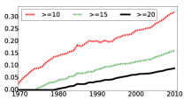
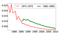
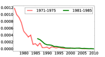
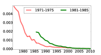
(a)	(b)	(c)	(d)

Figure 1. (Best viewed in color) a. For a paper written in $y\in[1970,2010]$ (x-axis), we plot the fraction of papers it cites (y-axis) that are older than $y-t$ years, for $t=10,15,20$ (red, green, black). b. We picked a fixed set $P$ of 100 most cited papers written in 1971–1975 (red) and 1981-1985 (green). For papers written in years $y\in[1975,2010]$ (x-axis), we plot the fraction (y-axis) of citations made to papers in $P$. Unlike (a), this shows a steep decrease. c. Replacing popular papers $P$ with a random set $R$ of papers written in 1971–1975 (red) and 1981–1985 (green) reduces the absolute y-axis but not the relative decay. d. Enlarging $R$ to 500 random papers also has no effect on the relative rate of decay.

2. Dataset

Investigating the questions raised in this work requires rich trajectories of time-stamped network snapshots. However, such intricately detailed datasets are rare, even while there are an increasing number of new repositories being built and updated regularly. Fortunately, Microsoft Academic Search (MAS) provides an ideal platform for our study. MAS data includes paper titles, reconciled paper IDs, year of publication, publication venue, references, citation contexts, related field(s), abstract and keywords, author(s) and their affiliations (Chakraborty et al., 2014). We have filtered papers from full dataset (Table 2). The filtered dataset consists of papers published between 1961–2010 and have at least one outlink or one inlink (to filter isolated nodes or missing data). We call this filtered dataset as the Ground Truth dataset (GT). For each simulation initialization, we create a warmup dataset from GT having papers published between 1961–1970. Detailed description and the role of warmup data in the simulation framework can be found in Section 5.2.

Table 2. General statistics about the full Computer Science dataset from Microsoft Academic Search. Filtered and warmup dataset are subsets of full dataset.

	Full	Filtered	Warmup
Year range	1859–2012	1961–2010	1961–1970
Number of papers	2,281,307	1,702,471	9,568
Number of citations	27,527,432	15,791,272	7,312

To ensure that our proposed temporal signatures are generally applicable, we also experimented with papers from the biomedical domain. In this study, we use biomedical dataset that consists of 801,252 research articles published between 1996-2014. All our evaluations are based on extensive experiments with the Computer Science domain dataset.

3. Entrenchment and obsolescence

Preferential attachment models without aging (Jeong et al., 2003; Kumar et al., 2000) predict that older papers get more entrenched and their rate of citation acquisition can only go up. Verstak et al. (Verstak et al., 2014) provide support that as a cohort older papers are thriving: more recently written papers have a larger fraction of outbound citations targeting papers that are older by a fixed number of years. However, there is plenty of evidence (Chakraborty et al., 2015; Wang et al., 2013; Wang et al., 2009) that aging counteracts entrenchment. This apparent contradiction is readily resolved by realizing that the number of papers older by a fixed number of years is growing rapidly. But the real value of the study (Sections 3.1 and 3.2) is that it leads us to the definition of new signatures of evolving networks (Section 4).

3.1. Fraction of citations to ‘old’ papers

Suppose that papers in our corpus, published in year $y$, make $C_{y}$ citations in all to older papers. Of these, say $C_{t}$ citations go to papers that were published before year $y-t$, for $t=10,15,20$. Figure 1(a) plots the quantity ${C_{t}}/{C_{y}}$ against $y$, similar to the setup of Verstak et al. (Verstak et al., 2014). The plot is consistent with their claim: the fraction of citations to older papers is indeed increasing over the years $y$ for all values of $t$.

However, Figure 1(b) paints a different picture. For each year range 1971–1975 and 1981–1985, we choose 100 most cited (through 2010) papers $P$. Then, for other papers written in year $y\in[1975,2010]$, we plotted the fraction of citations out of those papers that go to $P$. Clearly, this fraction decreases over time. In place of popular papers, how do random papers fare? Figures 1(c,d) show that the relative shape of decay remains stable when random paper sets of sizes 100 and 500 are picked as the targets.

3.2. Fraction of citations to papers in 10-year age buckets

Figures 1 suggests a natural and compact way to summarize citation statistics organized by age. We group papers into buckets. Each bucket includes papers published in one decade. Then, for each bucket, we plot as a stacked bar-chart, the fraction of citations going to that same bucket as well as all previous buckets. Figure 3a shows the result. We note the following:

• The fraction of citations from a bucket to itself (shown as the bottom purple, yellow, red and blue bars in successive columns) decreases over time, and those to all older buckets increases over time. This is consistent with Verstak et al.

• However, if we consider papers in a bucket as targets, the citations they receive decreases over the years. For instance, papers written in 1971–1980 (purple bars over successive columns) received 70.5% of the citations in that decade (purple) but this number reduces to $29.2,6.4,2.8$% in successive decades. Similar decay is seen for the following buckets (yellow, red) as well.

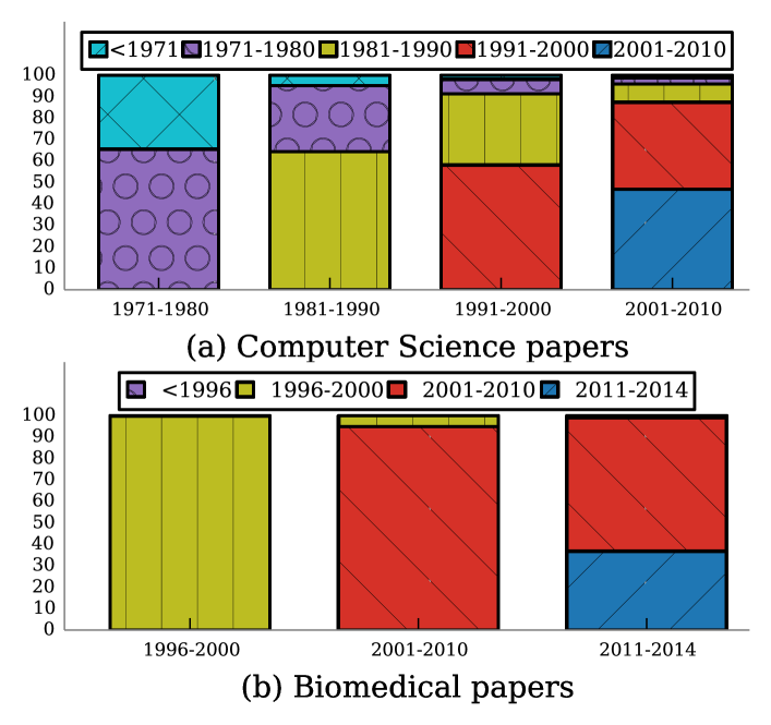
Figure 3. a. Citation distribution across 10-year buckets for computer science dataset. Each vertical bar represents a decade of papers. Within each bar, colored/textured segments represent the fraction of citations going to preceding decades. The bottommost segment is to the same decade, the second from bottom to the previous decade, etc. On one hand, the volume of citations to the current decade (bottommost segment) is shrinking to accommodate “old classics” (entrenchment). On the other hand, any given color/texture shrinks dramatically over decades (most papers fade away). b. Citation distribution for biomedical dataset. Papers written in 1996–2000 became obsolete much more rapidly.

We see similar effects in Figure 3(b), except that papers written in 1996–2000 became obsolete much more rapidly (yellow bar) compared to papers written in 2001–2010, so there is less stationarity of the obsolescence process in the biomedical domain compared to computer science. Thus, such bar charts simultaneously validate Verstak et al. (Verstak et al., 2014) and also show aging of paper cohorts, and are a succinct signature of the balance between entrenchment and obsolescence.

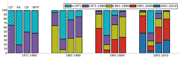
Simulator Distance Turnover Divergence GT – 2.70 – PA 4.98 0.97 0.77 CP ($p_{\text{copy}}=.5$) 1.97 1.53 0.18 WYY ($\lambda=.11$) 1.67 2.59 0.13

Figure 4. Temporal bucket signatures comparing ground truth (GT), preferential attachment (PA), copying (CP) and WYY, the model proposed by Wang et al. (Wang et al., 2009). Each bucket represents a decade. Ground truth turnover is 2.70. For others, distance, turnover and divergence values are shown in the accompanying table. Clearly, only WYY has even a remote similarity to ground truth.

4. New signatures of evolving networks

We start with some basic notation. Time $t$ proceeds in discrete steps (for publications, often measured in years). Sometimes we will bucket time into ranges like decades. We study an evolving graph $G_{t}$, which comprises the node set $V_{t}$ and edge set $E_{t}$. Nodes are denoted by $u,v$, etc. Edges (i.e., citations) once added, are never removed. Also, in our bibliometric setting, edges emanating from a node $v$ all “appear” when node $v$ itself appears, at birth time $t_{v}$, but this assumption can be relaxed. We shall use GT as the shorthand for ground-truth data (see Section 2).

We introduce several natural ways to observe dynamic networks to better understand the interplay between entrenchment and obsolescence.

4.1. Age gap count histogram

When new paper $u$, born at time $t_{u}$, cites an older paper $v$, born at $t_{v}$, that citation link spans an age gap of $t_{u}-t_{v}\geq 0$. (Depending on the granularity of measuring time, $t_{u}=t_{v}$ may or may not be possible.) In case of dynamic documents where $u$ can add citations (dropping citations is rare), we can take $t_{u}$ to be the citation creation time, rather than the birth time of $u$. In citation data, gap $g$ is usually expressed in whole years. For any value of $g$,

(1) $$\sum_{(u,v)\in E}\begin{cases}1,&\text{if $t_{u}-t_{v}=g$, and}\\ 0,&\text{otherwise}\end{cases}$$

is the number of links that span an age gap of $g$. As we shall see later, age gap count histograms reveal some salient dynamics of graph evolution.

4.1.1. Divergence

Suppose we observe age gap histograms $H$ from real data. Each simulated model gives age gap histograms $\tilde{H}$. We assess divergence between two histograms ($\tilde{H}$ and $H$) by measuring Kullback-Leibler divergence. More precisely,

(2) $$\text{divergence}(H||\tilde{H})=\sum_{g\in H}H(g)\log{\frac{H(g)}{\tilde{H}(g)}}$$

A simulated model is closer to real data, if $\text{divergence}\rightarrow 0$.

4.2. Temporal bucket signature

Suppose we collect birth times into buckets of temporal width $T$ (e.g., $T$ may be 10 years). Suppose our corpus of papers $P$ is thus partitioned into $P_{1},P_{2},\ldots,P_{N}$, based on their publication date. We pad this with sentinel bucket $P_{0}$ for all papers before $P_{1}$. Each source paper $p_{s}\in P_{j}$ may cite target papers $p_{t}\in P_{i}$, where $i\leq j$. Let the total number of citations from papers in $P_{j}$ to papers in $P_{i}$ be $C(i,j)$ (row=cited, column=citing). Let column sums $C(j)=\sum_{i}C(i,j)$ be the total number of outbound citations from papers in $P_{j}$. Let $F(i,j)=C(i,j)/C(j)$ be the fraction of outbound links from papers in $P_{j}$ that target papers in $P_{i}$. The temporal bucket signature is defined as the matrix $F(i,j):i\leq j$, i.e.,

(3) $$F =\begin{bmatrix}F(0,1)&F(0,2)&\cdots&F(0,N)\\ F(1,1)&F(1,2)&\cdots&F(1,N)\\ 0&F(2,2)&\cdots&F(2,N)\\ \vdots&0&\ddots&\vdots\\ 0&0&0&F(N,N)\end{bmatrix},$$

where each column adds up to 1. We propose two intuitive scalar summaries of temporal bucket signatures.

4.2.1. Distance

Suppose we observe $F$ from real data. We also fit a model which, upon simulation, gives bucket signature $\tilde{F}$. We propose to assess how closely $\tilde{F}$ approximates $F$ by measuring the average row-wise L1 distance between their corresponding columns. More precisely,

(4) $$\text{distance}(F,\tilde{F}) =\sum_{j=1}^{N}\left[\sum_{i=0}^{j}|F(i,j)-\tilde{F}(i,j)|\right].$$

The higher the distance value, lower will be the closeness of approximation, and vice versa. Note that there is no assumption of stationarity in this definition. Communities can be in volatile and transient stages of obsolescence while replacement rates in other communities can be stable.

4.2.2. Turnover

Another quantity of interest summarizing $F$ or $\tilde{F}$ is a notion of decay of the height of a segment of a given color from one column to the next, in the sequence $F(i,i),F(i,i+1),F(i,i+2),\ldots$ Specifically, the ratio $F(i,j)/F(i,j+1)$ (which is usually more than 1) represents how sharply citations to papers in $P_{i}$ decreases from year $j$ to year $j+1$. Because we are interested in a ratio, we aggregate these via a geometric mean:

(5) $$\text{turnover}(F) =\left[\prod_{j=1}^{N-1}\prod_{i=0}^{j}\frac{F(i,j)}{F(i,j+1)}\right]^{\frac{2}{(N+2)(N-1)}}$$

A high value of turnover indicates more rapid obsolescence. Turnover can be measured on both $F$ and $\tilde{F}$. In the later sections, we will relate the quantities we have defined with other established properties of real networks.

4.3. Optimization

We assume that the temporal bucket signature for GT is $F$ and the age gap histogram is $H$. Similarly, for each simulated model, we denote $\tilde{F}$ and $\tilde{H}$ as temporal bucket signature and age gap histogram respectively. Note that, $\tilde{F}$ and $\tilde{H}$ are dependent on two model parameters $\lambda$ and $\Theta$ (see Figure 7). We use $d(\cdot)$, $t(\cdot)$ and $f(\cdot)$ as shorthand for $\text{distance}(\cdot)$, $\text{turnover}(\cdot)$ and $\text{divergence}(\cdot)$ respectively. To obtain optimal set of parameters for each model, we need to solve the following optimization problem:

(6) $$\underset{\lambda,\theta}{\text{minimize}} \emph{d}(F,\tilde{F})*\left(|t(\tilde{F})-t(F)|\right)*f(H||\tilde{H})$$

Here, $|t(\tilde{F})-t(F)|$ represents absolute difference between GT’s turnover (e.g., 2.70 for one of our data sets), and relay-link model’s turnover. Other combinations such as weighted sums can be considered, but product has the advantage that we do not need to manually balance typical magnitudes of the parts. To our knowledge the above problem does not admit a tractable continuous optimization procedure. Therefore, we perform grid search and choose values for model parameters for each proposed model.

5. Classical evolution models and simulation results

The first generation of idealized network growth models (Albert and Barabási, 2002; Pennock et al., 2002) generally focused on a “rich gets richer” (preferential attachment or PA) phenomenon without any notion of aging. This was followed by the vertex copying model (Kumar et al., 2000). There has been more recent work (Dorogovtsev and Mendes, 2000; Hajra and Sen, 2005; Wang et al., 2013; Wang et al., 2009; Zhu et al., 2003) on modeling age within the PA framework. We will review and evaluate some of these in Section 5.2.

5.1. Classical Models

5.1.1. Standard preferential attachment (PA)

In Albert et al.’s classical PA model (Albert and Barabási, 2002; Jeong et al., 2003), at time $t$, a new paper would cite an old paper $p$, which currently has degree $k_{p}(t)$, with probability $\Pi(p,t)$ that is proportional to $k_{p}(t)$:

(7) $$\Pi(p,t)\propto k_{p}(t)$$

In their idealized model, one new paper was added at every time step, but this is easily extended to mimic and match the growing observed rate of arrival of new papers. Moreover, the number of outbound citations from each new paper can also be sampled to match real data.

If paper $p$ arrives at time $t_{p}$, it is not hard to obtain a mean-field approximation to the degree of $p$ at time $t\geq t_{p}$:

(8) $$\tilde{k}_{p}(t)\propto\sqrt{t/t_{p}}.$$

This expression suggests that age is a monotone asset, never a liability, for any paper.

5.1.2. Copying model (CP)

The copying model (Kumar et al., 2000) is characterized by a network that grows from a small initial graph and, at each time step, adds a new node (paper) $p_{n}$ with $k$ edges (citations) emanating from it. Let $p_{r}$ be a “reference” paper chosen uniformly at random from pre-existing papers. With a fixed probability (the only parameter of the model), each citation from $p_{n}$ is assigned to the destination of a citation made by $p_{r}$, i.e., $p_{n}$ “copies” $p_{r}$’s citations. Neither PA nor copying has a notion of aging.

5.1.3. Ageing model (WYY)

Wang, Yu and Yu (Wang et al., 2009) proposed modeling age within the PA framework. The probability of citing at time $t$ a paper $p$ that was born at time $b_{p}$, while proportional to its current degree as in PA, decreases exponentially with its age:

(9) $$\Pi(p,t) \propto k_{p}(t)\,\exp\Bigl{(}-\lambda(t-b_{p})\Bigr{)},$$

where $\lambda>0$ is the single global parameter controlling the attention decay rate, estimated from some “warmup” data. Similar models are motivated by the measurements by Leskovec et al. (Leskovec et al., 2008). Note, in order to avoid huge computational overhead associated with updating probability values for each new entry, we approximate by only updating the attachment probability value once in each year. For the first 20 years, the approximate version is (a) extremely close to the original version (less than .05 L1 distance) and (b) slightly closer to the GT than the original version thus giving this baseline a small additional advantage.

5.2. Simulation protocol and results

We simulate the models described above for 40 years (1971–2010) and compare the results with GT ($turnover=\textbf{2.70}$). Warmup data is the subset of GT generated between 1961–1970 (detailed statistics is present in Section 2). Warmup data consists of papers published between 1961–1970 along with the citation links formed between them. We initiate each simulation model from warmup data. The warmup data can be called as the “train data”. Starting from the year 1971, for each subsequent year we introduce as many papers in the system as the publication count of that year estimated from GT. Each incoming paper is accompanied by nine outlinks (average number references estimated from GT). This data, generated through our simulation models between 1971–2010, can be called as “test data”. We simulate CP with copying probability = 0.5 (after grid search on all possible probability values) since the product of the three observables, i.e., distance, turnover, and divergence (a function similar to (6)) is the least at this value of the probability. Similarly, for WYY, we obtain through grid search $\lambda=0.11$ that results in the lowest product of the three observables.

Results are shown in Figure 4. PA fits observed temporal bucket profiles very poorly. The distance score is very large (4.98). Neither PA nor copying has a notion of aging. Therefore, it is not surprising that CP also does not fit observed temporal bucket signatures well. The distance score is 1.97. WYY performed best at $\lambda=0.11$ with distance = 1.67. As for turnover, WYY’s turnover (2.59) is closest to that of GT (2.70).

5.3. Other related models

5.3.1. Forest Fire

Relay-linking has some superficial similarity to the forest fire model (Leskovec et al., 2005) and earlier work on random walk and recursive search based attachment processes (Vazquez, 2001). But among many critical difference is the involvement of time and node ages. In forest fire terminology, the relative birth times of candidate source and target nodes strongly influence whether we prefer to ‘burn’ forward or backward edges. To our knowledge, there is no similar temporally modulated version of forest fire model that has demonstrated fidelity to bucket signatures, or age gap count histograms.

5.3.2. Point processes

It is attractive to think of citations as events “arriving at a node/paper” according to some temporal point process. Focusing on one node, if $\mathcal{H}(t)$ is the history of event arrivals up to time $t$, then the conditional intensity function is defined as

$$\gamma(t)dt :=\Pr(\text{event in $[t,t+dt)$}|\mathcal{H}(t)).$$

Specifically, if $\mathcal{H}_{v}(t)$ comprises the points of time ${t_{vi}<t}$ of past arrivals at node $v$, then the Hawkes process (Aalen et al., 2008) defines

$$\gamma_{v}(t) =a_{v}+b_{v}\sum_{t_{vi}<t}\exp(-|t-t_{vi}|).$$

and provides two major benefits: (1) the exponential decay term elegantly captures temporal burstiness, and (2) given $\{t_{vi}\}$, parameters $a_{v},b_{v}$ can be estimated efficiently (Bacry et al., 2015; Farajtabar et al., 2015). While Hawkes process is most suited for repeated similar events (such as messages or tweets between two people), citation happens only once between two papers. Work on coupling edge message events to network evolution itself is rare, with notable exceptions (Farajtabar et al., 2015). In our case, citation arrivals at different papers are not independent events, but coupled to global population growth rates as well as network constraints (e.g., out-degree distribution). Given those constraints, Hawkes process provides no obvious benefits to inference or simulation. Moreover, citations are often observed in (annual) batches, but Hawkes process finds simultaneous arrivals impossible. We can model arrival times as hidden and observe them in batches, but that involves a more complex EM procedure (Liu et al., 2015) to marginalize over arrivals. Even if these hurdles can be overcome, we have to estimate or sample $a_{v},b_{v}$ for every node, just like WSB (Wang et al., 2013), which results in too many parameters. Moreover, there is still no direct connection between declining citations and whether the network guides the diverted citations to specific targets, which is the specific goal of relay-linking models.

6. Proposed relay-linking models

6.1. Evidence of citation stealing

The central hypothesis behind the relay linking model is as follows:

At a given point in time, an old popular paper $p_{0}$ begins to lose citations in favor of a relatively young paper $p_{1}$ that cites $p_{0}$.

There are a variety of intuitive reasons why relay-linking or relay-citing can happen:

• $p_{1}$ is a journal version of a conference paper $p_{0}$,

• $p_{1}$ refutes or improves upon $p_{0}$, or

• $p_{1}$ reuses data or a procedure in $p_{0}$, and so on.

Table 5. Circumstantial evidence of relay-link: $R_{W}$ papers acquire more citations than $R_{L}$ papers. Here, $r$ is in $R_{W}$ or $R_{L}$ . Higher proportion of papers belonging to $R_{L}$ have zero citation count than $R_{W}$. Bold face text represents that the mean of cumulative citation count of $R_{W}$ at base year $T$ is larger than the mean of $R_{L}$. Also, $R_{W}$ papers show higher increasing trend than $R_{L}$ papers.

	Popularity of cited papers	#Papers	#Papers with $>0$ citations	%Papers with $>0$ citations	Avg #citations to $r$	#Recent papers with increasing trend	%Recent papers with increasing trend	Cited neighbors with decreasing trend (%)	Avg. decrease in median values
$R_{W}$	$\geq 70$	76082	60205	79.13	19.77	31749	41.72	48.06	5.69
$R_{L}$	$\leq 10$	16257	2017	12.40	0.31	736	4.52	41.39	0.41

Table 6. Circumstantial evidence of relay-link: Papers that cite fading papers gather citations at an accelerated pace. Bold face text represents that the rate at which the citations are gained by the set of $R^{\prime}$ papers is higher compared to the set of $R_{W}\setminus R^{\prime}$ papers.

$R_{W}$			$R^{\prime}$			$R_{W}\setminus R^{\prime}$
#papers in $P_{P}$	#papers in F	Avg. drop	Avg. citation count at T	Avg. citation gain in $[T,T+\delta T]$	Per-year citation gain	Avg. citation count at $T$	Avg. citation gain $[T,T+\delta T]$	Year-wise citation gain
21621	4962	36.41	23.48	13.92	2.48	11.02	11.89	2.05

Unlike standard preferential attachment (PA), evidence for relay-linking can only be circumstantial and in the aggregate, because the decision of $p_{2}$ to select, but then not cite $p_{0}$, is never recorded in any form; we get to know only of the recorded citation to $p_{1}$. Here we produce such circumstantial evidence, in two parts.

Fix a base time $T$ (2005 in our experiments). Define popular papers $P_{P}$ as those that have at least 70 cumulative citations as of $T$. Define obscure papers $P_{O}$ as those that have at most ten cumulative citations as of $T$. Let recent winner papers $R_{W}$ be those that make at least ten citations and at least 50% are to papers in $P_{P}$. Let recent loser papers $R_{L}$ be those that make at least ten citations, and all are to papers in $P_{O}$.

Do $R_{W}$ papers gain citations faster than $R_{L}$?

We now measure the cumulative citations to each paper in $R_{W}$ and $R_{L}$ as of time $T+\delta T$ (say after five years), and can apply a standard test of the hypothesis that the mean of $R_{W}$ is larger than the mean of $R_{L}$ (see Table 5).

Are $R_{W}$ papers stealing citations from $P_{P}$ papers?

Now we focus on a subset of $P_{P}$: those whose rate of acquiring citations see a sharp ($>50\%$) drop from $[T-\delta T,T]$ to $[T,T+\delta T]$. Let this be fading papers $F\subset P_{P}$. Consider papers $R^{\prime}\subset R_{W}$ that cite papers in $F$, and their rate of acquiring citations in $[T,T+\delta T]$. We investigate if this population has a significantly larger mean than a base population. Here the base population are set to the papers $R_{W}\setminus R^{\prime}$. In Table 6 we observe that indeed the rate at which the citations are gained by the set of $R^{\prime}$ papers is higher compared to the set of $R_{W}\setminus R^{\prime}$ papers.

6.2. Model descriptions and results

Inspired by the above experiments, we propose in Fig. 7, a generic template for all our relay-link models. $t_{u}$ is the birth time of $u$. The flexible policies/ parameters are $R,\lambda,\Theta,D$. $R$ is either 1 (one-shot relay) or $\infty$ (iterated relay). $D$ is either uniform, or as in PA, but restricted to $I(u,t)$. The $\lambda$ parameter governs the time to initiate relaying while the $\Theta$ parameter governs the extent of relaying. Higher value of $\lambda$ leads to relaying of citations from source paper soon after its publication and vice-versa. Similarly, $\Theta$ controls intensity of relaying; higher values of $\Theta$ lead to higher intensity of relaying. Note that, standard PA can be achieved by keeping $\lambda=0$. We will explore alternatives for a few design choices, and that will lead us to a few variations on the basic theme.

6.2.1. Random relay-cite (RRC)

Our first model is obtained by setting $R=1$ and $D$ as the uniform distribution over $I(u,t)$. In words, we first pick a $p_{0}$ to cite, then we toss a coin with head probability = $exp(-\lambda T)$, where T is the current age of the paper $p_{0}$. If the coin turns up tail, then again, we toss a coin with head probability $\Theta$. With coin turning up as head, we sample a paper $v$ that links to $p_{0}$ uniformly at random, and then cite $v$ instead of $p_{0}$. Effectively, $p_{0}$ relays the citation to $v$. This version of the model thus has two parameters $\lambda$ and $\Theta$.

We simulated the model with different values of $(\lambda,\Theta)$. Grid search led us to the best value of $(0.19,0.9)$ as per the optimization function defined in  (6). Figure 8 shows the temporal bucket signatures for this and the other variants described below; the best distance, turnover and divergence that RRC achieves are 1.08, 2.70 and 0.03.

1:for advancing time steps $t$ do 2:     for each paper $p_{n}$ newly added at time $t$ do 3:         for each citation $(p_{n},?)$ to fill do 4:              choose old paper $u$ using PA 5:              for $r=1,2,\ldots$ do 6:                  $T=t-t_{u}$ 7:                  toss coin with head prob. $\exp(-\lambda T)$ 8:                  if head or $r>R$: break 9:                  toss coin with head prob. $\Theta$ 10:                  if tail: break 11:                  let $I(u,t)$ be papers that cite $u$ 12:                        as of time $t$ 13:                  choose $v\in I(u,t)$ according to 14:                        a sampling distribution $D$ 15:                  $u\leftarrow v$                16:              add $(p_{n},u)$ as new citation               

Figure 7. Relay-linking template.

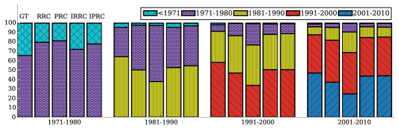
Simulator ($\lambda,\Theta$) Distance Turnover Divergence RRC (0.19, 0.9) 1.08 2.70 0.03 PRC (0.3, 0.9) 1.86 2.11 0.16 IRRC (0.115, 0.8) 0.60 2.67 0.012 IPRC (0.19, 0.8) 0.72 2.70 0.004

Figure 8. Temporal bucket signatures from ground truth data (GT), random relay-cite (RRC), preferential relay-cite (PRC), iterated RRC (IRRC) and iterated PRC (IPRC). $\lambda$ and $\Theta$ were optimized separately for each variant using grid search. Ground truth turnover is 2.70. For others, distance, turnover and divergence values are shown in the accompanying table. Note the qualitatively better fit with ground truth compared to Figure 4.

6.2.2. Preferential relay-cite (PRC)

In the preferential relay-cite model, $R$ continues to be 1, but we depart from the random relay-cite model in that $D$ is no more a uniform distribution over the papers in $I(u,t)$. The probability of sampling $v$ is proportional to its in-degree, as in PA. Again, we simulated this model and performed a grid search to obtain the best parameter values $(\lambda,\Theta)=(0.3,0.9)$ as per the optimization function in Equation 6. We obtained the best distance score of 1.86. The corresponding turnover and divergence scores were found to be 2.11 and 0.16.

6.2.3. Iterated random relay-cite (IRRC)

In iterated random relay-cite model, we relax $R$ to be able to follow the relay-cite hypothesis iteratively. Thus, once a paper $v$ has sampled a paper from $I(u,t)$ based on uniform distribution, we again toss a coin with head probability = $\exp(-\lambda T^{\prime})$, where $T^{\prime}$ is the current age of the paper $v$. In case, tail turns up, we follow this process recursively. $(\lambda,\Theta)=(0.115,0.8)$ gives the best distance score of 0.60, turnover of 2.67 and divergence score of 0.012.

6.2.4. Iterated preferential relay-cite (IPRC)

In iterated preferential relay-cite model, once a paper $v$ has sampled a paper from $I(u,t)$ based on PA, we again toss a coin with head probability = $\exp(-\lambda T^{\prime})$, where $T^{\prime}$ is the current age of the paper $v$. In case, tail turns up, we follow this process recursively. We simulated the model with different parameter values, and found that $\lambda=0.19$ and $\Theta=0.8$ gives the best distance score of 0.72, turnover score of 2.70 and divergence score of 0.004.

6.3. Dependence on bucket size

Since divergence is computed from age gap count histograms, it does not depend on the bucket size. For distance and turnover, we observed that our observations are stable for bucket sizes 7, 8 and 9 years. For bucket sizes larger than 10 years, the number of buckets is too small to make a fair comparison.

7. Comparison between models

7.1. Temporal bucket signatures

Fig. 8 compares ground truth (GT) temporal bucket signatures against the variations of relay-linking models described above. Three out of four relay-linking models proposed above outperform the popular baseline models of network evolution in terms of all the observables, i.e., distance, turnover and divergence (see Figure 4 for detailed result obtained for the baseline models.) Further, note that IPRC outperforms all the other relay-linking models in at least two out of the three observables and can be considered to be the closest fit to GT. Therefore, in order to strengthen our results, we compare age gap count histograms and degree distribution of IPRC (instead of other relay-linking models) with the baseline models.

7.2. Age gap count histograms

Fig. 9 shows the age gap count histograms defined in equation (1) for various simulators, compared with ground truth (over all time). Ground truth rolls down steadily after an early peak at 2–3 years age gap. As expected, the PA curve keeps going up, because aging is always an advantage. Surprisingly, but indirectly corroborating degree distribution (as well as its temporal signature in Figure 4), WYY does well in comparison, but its most likely gap is larger compared to real data. IPRC fits GT’s decay best.

The model complexity of relay-linking is comparable to PA. Yet, we establish that relay-linking is the closest to real networks in terms of divergence, distance, and turnover.

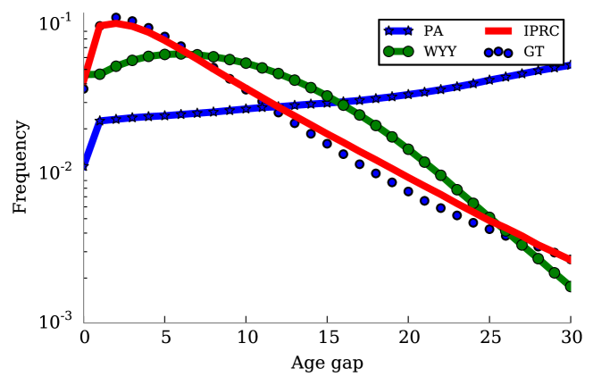
Figure 9. Age gap count histograms. WYY is quite close to ground-truth, but for its best choice of $\lambda$, its peak is still at too large a gap. IPRC’s decay fits GT best. The divergence values are, PA: 0.77; WYY($\lambda=0.11$): 0.13; IPRC ($\lambda=0.19,\Theta=0.8$): 0.004

7.3. Degree distribution

We also find it remarkable that relay-linking models fit temporal bucket signatures better than all other models. In Figure 10 we plot the degree distribution of the network obtained by simulating IPRC. The figure shows that the distribution fits the GT quite well. We should, however, verify that other properties of real networks that are matched well by preferential attachment or similar models are preserved.

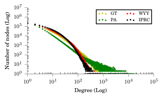
Figure 10. Degree distributions of ground truth (GT) and various models (PA,WYY,IPRC) at the best optimal parameters values.

8. Practical Application

To get more insight into temporal bucket signatures, we apply these to a cross-sectional study by sub-field and conference slices. The widely quoted impact factor (Garfield, 2006) (IF10) of a journal or conference is the average number of citations to recent (last 10 years) articles published there. Table 11 shows the turnover values we estimate against IF10 for the four conference subsets we chose. There is a clear negative correlation i.e., communities with large turnover have low IF10. Large turnover also seems associated with applied communities in a state of more intense flux.

Table 11. Correlation between turnover and average value of 10-year impact factor, over specific conferences as well as coherent sub-communities of computer science. Note the negative correlation between turnover and 10-year impact factor. Communities with large turnover have low IF10.

Conference Name	Turnover	Avg. IF10
SIGMOD	3.97	3.50
VLDB,ICDE	4.52	2.79
SIGIR	5.61	2.77
ICML,NIPS	6.74	1.84
Data Mining, machine learning, artificial intelligence, natural language processing and information retrieval	3.32	0.63
Distributed and parallel computing, hardware and architecture, real time and embedded systems	3.31	0.74
Algorithms and Theory, Programming Languages and Software Engineering	2.29	0.78

9. Conclusion

Idealized network evolution models that explain entrenchment of prominence are abundant, but the only ones that model aging depend on post-hoc distribution-fitting (data collapse) and externality (fitness) parameters. We give the first plausible network-driven models for obsolescence in the context of research paper citations, based on a natural notion of relay-linking. Studying large bibliographic data sets, we also propose several novel and stringent tests for temporal fidelity of evolving, aging network models. Traditional aging models do not pass these tests well, but our relay-linking models do.

Finally, a number of potential limitations need to be considered. First, the current study employs bibliographic datasets only. Therefore, we do not claim about generic applicability in other social networks. In future, we plan to extend this study to other citation networks, for example, U.S. Supreme Court citation network. Second, our proposed relay models do not consider area/author information which might be relevant in deciding the relay citation. On account of the fact that the current work is only a preliminary attempt to understand the relaying phenomenon of citation links, future extensions could possibly lead to formal analysis of properties of relay-linking or tractable variations.

References

- (1)
- Aalen et al. (2008) Odd Aalen, Ornulf Borgan, and Hakon Gjessing. 2008. Survival and event history analysis: a process point of view. Springer.
- Albert and Barabási (2002) Réka Albert and Albert-László Barabási. 2002. Statistical mechanics of complex networks. Reviews of modern physics 74, 1 (2002), 47.
- Bacry et al. (2015) Emmanuel Bacry, Stéphane Gaïffas, Iacopo Mastromatteo, and Jean-François Muzy. 2015. Mean-field inference of Hawkes point processes. arXiv/1511.01512 (2015). http://arxiv.org/pdf/1511.01512.pdf
- Bhattacharjee and Seno (2001) Somendra M Bhattacharjee and Flavio Seno. 2001. A measure of data collapse for scaling. J. Physics A: Mathematical and General 34, 33 (2001), 6375. http://arxiv.org/pdf/cond-mat/0102515v2.pdf
- Chakraborty et al. (2014) Tanmoy Chakraborty, Suhansanu Kumar, Pawan Goyal, Niloy Ganguly, and Animesh Mukherjee. 2014. Towards a Stratified Learning Approach to Predict Future Citation Counts. In Proceedings of the 14th ACM/IEEE-CS Joint Conference on Digital Libraries (JCDL ’14). IEEE Press, 351–360.
- Chakraborty et al. (2015) Tanmoy Chakraborty, Suhansanu Kumar, Pawan Goyal, Niloy Ganguly, and Animesh Mukherjee. 2015. On the Categorization of Scientific Citation Profiles in Computer Science. Commun. ACM 58, 9 (Aug. 2015), 82–90. DOI:http://dx.doi.org/10.1145/2701412
- Cho et al. (2005) Junghoo Cho, Sourashis Roy, and Robert E Adams. 2005. Page quality: In search of an unbiased Web ranking. In SIGMOD conference. ACM, 551–562.
- Dalfovo et al. (1999) Franco Dalfovo, Stefano Giorgini, Lev P Pitaevskii, and Sandro Stringari. 1999. Theory of Bose-Einstein condensation in trapped gases. Reviews of Modern Physics 71, 3 (1999), 463.
- de Solla Price (1965) Derek J. de Solla Price. 1965. Networks of Scientific Papers. Science 149, 3683 (1965), 510–515. DOI:http://dx.doi.org/10.1126/science.149.3683.510 arXiv:http://science.sciencemag.org/content/149/3683/510.full.pdf
- Dorogovtsev and Mendes (2000) Sergey N Dorogovtsev and José Fernando F Mendes. 2000. Evolution of networks with aging of sites. Physical Review E 62, 2 (2000), 1842.
- Farajtabar et al. (2015) Mehrdad Farajtabar, Yichen Wang, Manuel Gomez-Rodriguez, Shuang Li, Hongyuan Zha, and Le Song. 2015. COEVOLVE: A Joint Point Process Model for Information Diffusion and Network Co-evolution. CoRR abs/1507.02293 (2015). http://arxiv.org/abs/1507.02293
- Garfield (2006) Eugene Garfield. 2006. The history and meaning of the journal impact factor. JAMA 295, 1 (2006), 90–93.
- Hajra and Sen (2005) Kamalika Basu Hajra and Parongama Sen. 2005. Aging in citation networks. Physica A: Statistical Mechanics and its Applications 346, 1 (2005), 44–48.
- Holme and Kim (2002) Petter Holme and Beom Jun Kim. 2002. Growing scale-free networks with tunable clustering. Phys. Rev. E 86 (2002), 026107–(1–5).
- Jeong et al. (2003) Hawoong Jeong, Zoltan Néda, and Albert-László Barabási. 2003. Measuring preferential attachment in evolving networks. EPL (Europhysics Letters) 61, 4 (2003), 567.
- Ke et al. (2015) Qing Ke, Emilio Ferrara, Filippo Radicchi, and Alessandro Flammini. 2015. Defining and identifying Sleeping Beauties in science. Proceedings of the National Academy of Sciences (2015), 201424329.
- Kumar et al. (2000) Ravi Kumar, Prabhakar Raghavan, Sridhar Rajagopalan, D Sivakumar, Andrew Tomkins, and Eli Upfal. 2000. Random graph models for the web graph.. In FOCS. 57–65.
- Leskovec et al. (2008) Jure Leskovec, Lars Backstrom, Ravi Kumar, and Andrew Tomkins. 2008. Microscopic evolution of social networks. In SIGKDD Conference. 462–470. http://www-cs.stanford.edu/people/jure/pubs/microEvol-kdd08.pdf
- Leskovec et al. (2005) Jure Leskovec, Jon Kleinberg, and Christos Faloutsos. 2005. Graphs over time: densification laws, shrinking diameters and possible explanations. In SIGKDD Conference. 177–187.
- Liu et al. (2015) Yu-Ying Liu, Shuang Li, Fuxin Li, Le Song, and James M Rehg. 2015. Efficient Learning of Continuous-Time Hidden Markov Models for Disease Progression. In NIPS. 3599–3607.
- Pandey et al. (2005) Sandeep Pandey, Sourashis Roy, Christopher Olston, Junghoo Cho, and Soumen Chakrabarti. 2005. Shuffling a stacked deck: the case for partially randomized ranking of search engine results. In VLDB conference. 781–792.
- Parolo et al. (2015) Pietro Della Briotta Parolo, Raj Kumar Pan, Rumi Ghosh, Bernardo A. Huberman, Kimmo Kaski, and Santo Fortunato. 2015. Attention decay in science. Journal of Informetrics 9, 4 (2015), 734 – 745. DOI:http://dx.doi.org/10.1016/j.joi.2015.07.006
- Pennock et al. (2002) David M Pennock, Gary W Flake, Steve Lawrence, Eric J Glover, and C Lee Giles. 2002. Winners don’t take all: Characterizing the competition for links on the web. PNAS 99, 8 (2002), 5207–5211.
- Polchinski et al. (1996) Joseph Polchinski, Shyamoli Chaudhuri, and Clifford V Johnson. 1996. Notes on D-branes. arXiv preprint hep-th/9602052 (1996).
- Price (1976) Derek De Solla Price. 1976. A general theory of bibliometric and other cumulative advantage processes. Journal of the American Society for Information Science 27, 5 (1976), 292–306. DOI:http://dx.doi.org/10.1002/asi.4630270505
- Vazquez (2001) A Vazquez. 2001. Disordered networks generated by recursive searches. Europhysics Letters 54, 4 (2001), 430–435.
- Verstak et al. (2014) Alex Verstak, Anurag Acharya, Helder Suzuki, Sean Henderson, Mikhail Iakhiaev, Cliff Chiung-Yu Lin, and Namit Shetty. 2014. On the Shoulders of Giants: The Growing Impact of Older Articles. CoRR abs/1411.0275 (2014). http://arxiv.org/abs/1411.0275
- Wang et al. (2013) Dashun Wang, Chaoming Song, and Albert-László Barabási. 2013. Quantifying long-term scientific impact. Science 342, 6154 (2013), 127–132.
- Wang et al. (2009) Mingyang Wang, Guang Yu, and Daren Yu. 2009. Effect of the age of papers on the preferential attachment in citation networks. Physica A: Statistical Mechanics and its Applications 388, 19 (2009), 4273 – 4276. DOI:http://dx.doi.org/10.1016/j.physa.2009.05.008
- Waumans and Bersini (2016) Michaël Charles Waumans and Hugues Bersini. 2016. Genealogical trees of scientific papers. PloS one 11, 3 (2016), e0150588.
- Zhu et al. (2003) Han Zhu, Xinran Wang, and Jian-Yang Zhu. 2003. Effect of aging on network structure. Physical Review E 68, 5 (2003), 056121.