Astronomy Letters, 2016, Vol. 42, No. 11, pp. 721–733.

Galactic Kinematics from Data on Open Star Clusters

from the MWSC Catalogue

V.V. Bobylev${}^{1},$ A.T. Bajkova¹ and K.S. Shirokova^1,2

¹ Pulkovo Astronomical Observatory, St. Petersburg, Russia

² St. Petersburg State University, St. Petersburg, Russia

Abstract—Open star clusters from the MWSC (Milky Way Star Clusters) catalogue have been used to determine the Galactic rotation parameters. The circular rotation velocity of the solar neighborhood around the Galactic center has been found from data on more than 2000 clusters of various ages to be $V_{0}=236\pm 6$ km s^-1 for the adopted Galactocentric distance of the Sun $R_{0}=8.3\pm 0.2$ kpc. The derived angular velocity parameters are $\Omega_{0}=28.48\pm 0.36$ km s^-1 kpc^-1, $\Omega^{\prime}_{0}=-3.50\pm 0.08$ km s^-1 kpc^-2, and $\Omega^{\prime\prime}_{0}=0.331\pm 0.037$ km s^-1 kpc^-3. The influence of the spiral density wave has been detected only in the sample of clusters younger than 50 Myr. For these clusters the amplitudes of the tangential and radial velocity perturbations are $f_{\theta}=5.6\pm 1.6$ km s^-1 and $f_{R}=7.7\pm 1.4$ km s^-1, respectively; the perturbation wavelengths are $\lambda_{\theta}=2.6\pm 0.5$ kpc $(i_{\theta}=-11^{\circ}\pm 2^{\circ})$ and $\lambda_{R}=2.1\pm 0.5$ kpc $(i_{R}=-9^{\circ}\pm 2^{\circ})$ for the adopted four-armed model $(m=4).$ The Sun’s phase in the spiral density wave is $(\chi_{\odot})_{\theta}=-62^{\circ}\pm 9^{\circ}$ and $(\chi_{\odot})_{R}=-85^{\circ}\pm 10^{\circ}$ from the residual tangential and radial velocities, respectively.

INTRODUCTION

When the Galaxy and its subsystems are studied, great significance is attached to the observational data quality. Open star clusters (OSCs) play an important role here, because the mean values of quite a few kinematic and photometric parameters derived from them are highly accurate, while fitting to appropriate theoretical isochrones based on probable cluster members allows one to reliably estimate the distances (with an error of about 20%) to OSCs and their ages.

Open star clusters are used as a tool for studying the interstellar dust (Trumpler 1930; Clayton and Fitzpatrick 1987; Joshi 2005), the vertical structure of the Galactic disk (Bonatto et al. 2006; Piskunov et al. 2006; Joshi 2007), its age (Twarog and Anthony-Twarog 1989; Phelps 1997; Chaboyer et al. 1999), the metallicity distribution in it (Netopil et al. 2016), the age–metallicity relation (Friel 1995; Chen et al. 2003), and the stellar evolution (Maeder and Mermilliod 1981; Moroni and Straniero 2002). The great importance of OSCs for determining the local parameters of the Galactic rotation curve (Glushkova et al. 1998; Zabolotskikh et al. 2002; Loktin and Beshenov 2003; Piskunov et al. 2006; Bobylev et al. 2007) and the parameters of the spiral density wave (Amaral and Lépine 1997; Popova and Loktin 2005; Loktin and Popova 2007; Naoz and Shaviv 2007; Bobylev et al. 2008; Lépine et al. 2008; Junqueira et al. 2015; Camargo et al. 2015) has long been recognized.

The various data on OSCs are continuously updated. The number of discovered clusters has increased considerably in recent years owing to the appearance of large-scale infrared photometric surveys. These include, for example, 2MASS (The Two Micron All Sky Survey; Skrutskie et al. 2006) or WISE (Wide-field Infrared Survey Explorer; Wright et al. 2010). The analysis of 2MASS data performed by various authors enlarged the list of OSCs (Koposov et al. 2005; 2008; Froebrich et al. 2007; Glushkova et al. 2010). WISE data have revealed 652 new OSCs (Camargo et al. 2016) that are virtually invisible in the optical band. The deep infrared VVV (VISTA Variables in the Via Lactea; Cross et al. 2012) survey has revealed 58 OSC candidates toward the central Galactic bulge (Borisova et al. 2014), with the limiting distance being about 11.75 kpc (the cluster VVV CL117). Such works open up new possibilities in studying the Galactic structure.

Infrared observations were also conducive to the appearance of large-scale catalogues of stellar proper motions. These include, for example, the XPM (Fedorov et al. 2009, 2011) or PPMXL (Röser et al. 2010) catalogues. In the new MWSC (Milky Way Star Clusters; Kharchenko et al. 2013) catalogue the mean proper motions were determined for $\sim$3000 OSCs using data from the PPMXL catalogue. It is important to note that the MWSC catalogue is complete within 1.8 kpc of the Sun, which is more than twice the completeness of the previous version of the catalogue compiled by these authors. The goal of this paper is to refine the rotation parameters of the Galaxy and its spiral structure using the latest data on open star clusters. For this purpose we use the MWSC catalogue.

DATA

The MWSC (Milky Way Star Clusters) catalogue was presented in Kharchenko et al. (2013). It contains photometric and kinematic data on 3006 Galactic objects (stellar associations, open and globular clusters).

The MWSC catalogue surpasses considerably the previous COCD catalogue of these authors (Kharchenko et al. 2005a, 2005b) in the number of open star clusters with age and distance estimates and kinematic data. To derive the mean proper motions of OSCs in MWSC, we used the stellar proper motions from the PPMXL catalogue (Röser et al. 2010), in which their random errors range from 4 to 10 mas yr^-1. In systematic terms, the PPMXL catalogue is an extension of the International Celestial Reference System (ICRS) to faint stars, because it is tied to the Hipparcos (1997) catalogue.

The stellar proper motions in the PPMXL catalogue were obtained from a completely different material than in the ASCC-2.5 catalogue (Kharchenko and Röser 2001), which served as a basis for deriving the mean proper motions of OSCs in the COCD catalogue. Therefore, with regard to the stellar proper motions, we have a completely new material to investigate the kinematics of OSCs. The CRVAD-2 compilation (Kharchenko et al. 2007) served to derive the mean line-of-sight velocities of OSCs in the MWSC catalogue, just as in the COCD catalogue. For some of the OSCs information from other lists and databases, for example, from the series of catalogues by Dias et al. (2002), was included in MWSC.

We supplemented the MWSC catalogue (Kharchenko et al. 2013) by new data from two more papers of these authors: Schmeja et al. (2014) on 139 high-latitude OSCs and Scholz et al. (2015) on 63 OSCs with new distance and age determinations. We do not use the MWSC objects with descriptors like “a”, “g”, “n”, and “s” (associations, globular clusters, nebulae, and asterisms). As a result, we produced a list of 2877 OSCs. For all these clusters there are estimates of their ages, distances, and proper motion components, while for 695 of them there are line-of-sight velocity estimates.

METHOD

We know three stellar velocity components from observations: the line-of-sight velocity $V_{r}$ and the two tangential velocity components $V_{l}=4.74r\mu_{l}\cos b$ and $V_{b}=4.74r\mu_{b}$ along the Galactic longitude $l$ and latitude $b$, respectively, expressed in km s^-1. Here, the coefficient 4.74 is the quotient of the number of kilometers in an astronomical unit by the number of seconds in a tropical year, and $r$ is the heliocentric distance of the star in kpc. The proper motion components $\mu_{l}\cos b$ and $\mu_{b}$ are expressed in mas yr^-1. The velocities $U,V,W$ directed along the rectangular Galactic coordinate axes are calculated via the components $V_{r},V_{l},V_{b}:$

$$\begin{array}[]{lll}U=V_{r}\cos l\cos b-V_{l}\sin l-V_{b}\cos l\sin b,\\ V=V_{r}\sin l\cos b+V_{l}\cos l-V_{b}\sin l\sin b,\\ W=V_{r}\sin b+V_{b}\cos b,\end{array}$$ (1)

where the velocity $U$ is directed from the Sun toward the Galactic center, $V$ is in the direction of Galactic rotation, and $W$ is directed to the north Galactic pole. We can find two velocities, $V_{R}$ directed radially away from the Galactic center and $V_{circ}$ orthogonal to it in the direction of Galactic rotation, based on the following relations:

$$\begin{array}[]{lll}V_{circ}=U\sin\theta+(V_{0}+V)\cos\theta,\\ V_{R}=-U\cos\theta+(V_{0}+V)\sin\theta,\end{array}$$ (2)

where the position angle $\theta$ obeys the relation $\tan\theta=y/(R_{0}-x),$ and $x,y,z$ are the rectangular heliocentric coordinates of the star (the velocities $U,V,W$ are directed along the corresponding $x,y,z$ axes). The velocities $V_{R}$ and $W$ barely depend on the pattern of the Galactic rotation curve. However, to analyze the periodicities in the tangential velocities, it is necessary to determine a smoothed Galactic rotation curve and to form the residual velocities $\Delta V_{circ}.$

To determine the parameters of the Galactic rotation curve, we use the equations derived from Bottlinger’s formulas, in which the angular velocity $\Omega$ is expanded into a series to terms of the second order of smallness in $r/R_{0}:$

$$\begin{array}[]{lll}V_{r}=-U_{\odot}\cos b\cos l-V_{\odot}\cos b\sin l-W_{\odot}\sin b+\\ +R_{0}(R-R_{0})\sin l\cos b\Omega^{\prime}_{0}+0.5R_{0}(R-R_{0})^{2}\sin l\cos b\Omega^{\prime\prime}_{0},\end{array}$$ (3)

$$\begin{array}[]{lll}V_{l}=U_{\odot}\sin l-V_{\odot}\cos l-r\Omega_{0}\cos b\\ +(R-R_{0})(R_{0}\cos l-r\cos b)\Omega^{\prime}_{0}+0.5(R-R_{0})^{2}(R_{0}\cos l-r\cos b)\Omega^{\prime\prime}_{0},\end{array}$$ (4)

$$\begin{array}[]{lll}V_{b}=U_{\odot}\cos l\sin b+V_{\odot}\sin l\sin b-W_{\odot}\cos b-\\ -R_{0}(R-R_{0})\sin l\sin b\Omega^{\prime}_{0}-0.5R_{0}(R-R_{0})^{2}\sin l\sin b\Omega^{\prime\prime}_{0},\end{array}$$ (5)

where $R$ is the distance from the star to the Galactic rotation axis:

$$R^{2}=r^{2}\cos^{2}b-2R_{0}r\cos b\cos l+R^{2}_{0}.$$ (6)

The quantity $\Omega_{0}$ is the angular velocity of Galactic rotation at the solar distance $R_{0},$ the parameters $\Omega^{\prime}_{0}$ and $\Omega^{\prime\prime}_{0}$ are the corresponding derivatives of the angular velocity, and $V_{0}=|R_{0}\Omega_{0}|.$ As experience shows, to construct a smooth Galactic rotation curve in the range of distances $R$ from 2 to 12 kpc, it will suffice to know two derivatives of the angular velocity, $\Omega^{\prime}_{0}$ and $\Omega^{\prime\prime}_{0}$. Note that the velocities $V_{R}$ and $\Delta V_{circ}$ must be freed from the peculiar solar velocity $U_{\odot},V_{\odot},W_{\odot}.$

It is important to know the specific distance $R_{0}.$ Gillessen et al. (2009) obtained one of its most reliable estimates, $R_{0}=8.28\pm 0.29$ kpc, by analyzing the orbits of stars moving around the massive black hole at the Galactic center. From a sample of masers with measured trigonometric parallaxes Reid et al. (2014) estimated $R_{0}=8.34\pm 0.16$ kpc; Bobylev and Bajkova (2014a, 2014b) and Bajkova and Bobylev (2015) found $R_{0}=8.3\pm 0.4$ kpc also from masers. Based on these determinations, we adopt $R_{0}=8.3\pm 0.2$ kpc in this paper.

The influence of the spiral density wave in the radial, $V_{R},$ and residual tangential, $\Delta V_{circ},$ velocities is periodic with an amplitude of $\sim$10 km s^-1. According to the linear theory of density waves (Lin and Shu 1964), it is described by the following relations:

$$\begin{array}[]{lll}V_{R}=-f_{R}\cos\chi,\\ \Delta V_{circ}=f_{\theta}\sin\chi,\end{array}$$ (7)

where

$$\chi=m[\cot(i)\ln(R/R_{0})-\theta]+\chi_{\odot}$$ (8)

is the phase of the spiral density wave ($m$ is the number of spiral arms, $i$ is the pitch angle of the spiral pattern, and $\chi_{\odot}$ is the Sun’s radial phase in the spiral density wave); $f_{R}$ and $f_{\theta}$ are the amplitudes of the radial and tangential velocity perturbations, which are assumed to be positive.

In the next step, we apply a spectral analysis to study the periodicities in the velocities $V_{R}$ and $\Delta V_{circ}.$ The wavelength $\lambda$ (the distance between adjacent spiral arm segments measured along the radial direction) is calculated from the relation

$$\frac{2\pi R_{0}}{\lambda}=m\cot(i).$$ (9)

Let there be a series of measured velocities $V_{R_{n}}$ (these can be both radial, $V_{R},$ and tangential, $\Delta V_{circ},$ velocities), $n=1,\dots,N,$ where $N$ is the number of objects. The objective of our spectral analysis is to extract a periodicity from the data series in accordance with the adopted model describing a spiral density wave with parameters $f_{R},f_{\theta},\lambda(i)$ and $\chi_{\odot}$.

Having taken into account the logarithmic behavior of the spiral density wave and the position angles of the objects $\theta_{n},$ our spectral (periodogram) analysis of the series of velocity perturbations is reduced to calculating the square of the amplitude (power spectrum) of the standard Fourier transform (Bajkova and Bobylev 2012):

$$\bar{V}_{\lambda_{k}}=\frac{1}{N}\sum_{n=1}^{N}V^{{}^{\prime}}_{n}(R^{{}^{\prime}}_{n})\exp\Bigl{(}-j\frac{2\pi R^{{}^{\prime}}_{n}}{\lambda_{k}}\Bigr{)},$$ (10)

where $\bar{V}_{\lambda_{k}}$ is the $k$th harmonic of the Fourier transform with wavelength $\lambda_{k}=D/k,$ $D$ is the period of the series being analyzed,

$$\begin{array}[]{lll}R^{{}^{\prime}}_{n}=R_{\circ}\ln(R_{n}/R_{\circ}),\\ V^{{}^{\prime}}_{n}(R^{{}^{\prime}}_{n})=V_{n}(R^{{}^{\prime}}_{n})\times\exp(jm\theta_{n}).\end{array}$$ (11)

The algorithm of searching for periodicities modified to properly determine not only the wavelength but also the amplitude of the perturbations is described in detail in Bajkova and Bobylev (2012).

The sought-for wavelength $\lambda$ corresponds to the peak value of the power spectrum $S_{peak}.$ The pitch angle of the spiral density wave is derived from Eq. (9). We determine the perturbation amplitude and phase by fitting the harmonic with the wavelength found to the observational data. The following relation can also be used to estimate the perturbation amplitude:

$$f_{R}(f_{\theta})=\sqrt{4\times S_{peak}}.$$ (12)

Thus, our approach consists of two steps: (i) the construction of a smooth Galactic rotation curve and (ii) a spectral analysis of both radial, $V_{R},$ and residual tangential, $\Delta V_{circ},$ velocities. Such a method was applied by Bobylev et al. (2008) to study the kinematics of young Galactic objects, by Bobylev and Bajkova (2012) to analyze Cepheids, and by Bobylev and Bajkova (2013, 2015a) to determine the Galactic rotation curve from massive OB stars.

RESULTS

The system of conditional equations (3)–(5) is solved by the least-squares method with weights of the form $w_{r}=S_{0}/\sqrt{S_{0}^{2}+\sigma^{2}_{V_{r}}},$ $w_{l}=S_{0}/\sqrt{S_{0}^{2}+\sigma^{2}_{V_{l}}}$ and $w_{b}=S_{0}/\sqrt{S_{0}^{2}+\sigma^{2}_{V_{b}}},$ where $S_{0}$ is the “cosmic” dispersion, $\sigma_{V_{r}},\sigma_{V_{l}},\sigma_{V_{b}}$ are the dispersions of the corresponding observed velocities. $S_{0}$ is comparable to the root-mean-square residual $\sigma_{0}$ (the error per unit weight) in solving the conditional equations (3)–(5); therefore, we adopted $S_{0}=15$ km s${}^{-1}.$ The OSC distance errors were assumed to be 20%.

Table 1: Kinematic parameters found from OSCs by method I for four age intervals

Parameters	$\lg t<7.7$	$\lg t:7.7-8.4$	$\lg t:8.4-8.8$	$\lg t>8.8$
$U_{\odot},$ km s-1	$9.74\pm 1.13$	$8.38\pm 1.01$	$10.06\pm 1.46$	$18.40\pm 2.00$
$V_{\odot},$ km s-1	$11.19\pm 1.38$	$13.48\pm 1.13$	$10.94\pm 1.57$	$15.43\pm 2.44$
$W_{\odot},$ km s-1	$6.19\pm 1.10$	$5.97\pm 1.02$	$6.91\pm 1.42$	$7.78\pm 2.14$
$\Omega_{0},$ km s-1 kpc-1	$28.60\pm 0.81$	$26.34\pm 0.87$	$24.64\pm 1.56$	$28.22\pm 1.54$
$\Omega^{{}^{\prime}}_{0},$ km s-1 kpc-2	$-4.04\pm 0.16$	$-3.51\pm 0.17$	$-3.61\pm 0.29$	$-3.29\pm 0.34$
$\Omega^{{}^{\prime\prime}}_{0},$ km s-1 kpc-3	$0.19\pm 0.13$	$0.40\pm 0.15$	$0.78\pm 0.17$	$0.20\pm 0.17$
$\sigma_{0},$ km s-1	15.7	13.7	15.9	21.0
$N_{\star}$	209	197	136	123
$N_{equation}$	600	563	386	316
$A,$ km s-1 kpc-1	$-16.66\pm 0.64$	$-14.57\pm 0.70$	$-15.00\pm 1.18$	$-13.64\pm 1.42$
$B,$ km s-1 kpc-1	$11.95\pm 1.03$	$11.78\pm 1.11$	$9.65\pm 1.96$	$14.59\pm 2.09$

Table 2: Kinematic parameters found from OSCs by method II for four age intervals

Parameters	$\lg t<7.7$	$\lg t:7.7-8.4$	$\lg t:8.4-8.8$	$\lg t>8.8$
$U_{\odot},$ km s-1	$11.42\pm 1.14$	$9.49\pm 0.97$	$11.74\pm 1.15$	$13.94\pm 1.09$
$V_{\odot},$ km s-1	$13.77\pm 1.50$	$13.64\pm 1.24$	$17.85\pm 1.33$	$21.96\pm 1.29$
$W_{\odot},$ km s-1	$6.53\pm 1.01$	$6.42\pm 0.85$	$7.19\pm 0.87$	$7.59\pm 0.87$
$\Omega_{0},$ km s-1 kpc-1	$28.71\pm 0.70$	$26.71\pm 0.72$	$28.49\pm 0.79$	$28.76\pm 0.64$
$\Omega^{{}^{\prime}}_{0},$ km s-1 kpc-2	$-3.75\pm 0.14$	$-3.38\pm 0.15$	$-3.92\pm 0.18$	$-3.33\pm 0.14$
$\Omega^{{}^{\prime\prime}}_{0},$ km s-1 kpc-3	$0.20\pm 0.11$	$0.17\pm 0.11$	$0.82\pm 0.09$	$0.27\pm 0.06$
$\sigma_{0},$ km s-1	20.2	18.2	21.0	26.0
$N_{\star}$	476	509	671	1221
$N_{equation}$	1016	1120	1338	2037
$A,$ km s-1 kpc-1	$-15.54\pm 0.60$	$-14.02\pm 0.64$	$-16.27\pm 0.73$	$-13.82\pm 0.56$
$B,$ km s-1 kpc-1	$13.17\pm 0.92$	$12.69\pm 0.97$	$12.22\pm 1.08$	$14.94\pm 0.85$

Method I

First we obtained a solution based on a sample of OSCs for which the space velocities $U,V,W$ could be calculated. As can be seen from Eqs. (1), such clusters must be provided with the proper motions, line-of-sight velocities, and distances. In this case, each OSC gives the three conditional equations (3), (4), and (5). There are a total of 695 such clusters in the MWSC catalogue. We selected the OSCs satisfying the following constraint on the magnitude of the total space velocity:

$$\begin{array}[]{lll}\sqrt{U^{2}+V^{2}+W^{2}}<150~{}\hbox{km s${}^{-1}$}.\end{array}$$ (13)

The $3\sigma$ criterion was applied in solving the conditional equations (3)–(5). Since the proper motion errors increase dramatically with distance, we restricted the use of clusters with proper motions to the radius $r=4$ kpc. The latter restriction cuts off only about 20 distant OSCs, while reducing considerably (by 2–3%) $\sigma_{0}.$ Based on our sample of 665 clusters, we found the following kinematic parameters by this method:

$$\begin{array}[]{lll}(U_{\odot},V_{\odot},W_{\odot})=(10.61,12.59,6.72)\pm(0.66,0.75,0.68)~{}\hbox{km s${}^{-1}$},\\ \Omega_{0}=~{}27.14\pm 0.53~{}\hbox{km s${}^{-1}$ kpc${}^{-1}$},\\ \Omega^{{}^{\prime}}_{0}=-3.69\pm 0.10~{}\hbox{km s${}^{-1}$ kpc${}^{-2}$},\\ \Omega^{{}^{\prime\prime}}_{0}=0.375\pm 0.067~{}\hbox{km s${}^{-1}$ kpc${}^{-3}$}.\end{array}$$ (14)

In this solution the error per unit weight is $\sigma_{0}=16.5$ km s^-1. For the adopted $R_{0}=8.3\pm 0.2$ kpc the linear Galactic rotation velocity $(V_{0}=|R_{0}\Omega_{0}|)$ is $V_{0}=225\pm 7$ km s^-1, while the Oort constants $(A=0.5\Omega^{\prime}_{0}R_{0}$ and $B=\Omega_{0}+0.5\Omega^{\prime}_{0}R_{0})$ are $A=-15.31\pm 0.43$ km s^-1 kpc^-1 and $B=11.83\pm 0.68$ km s^-1 kpc^-1

Table 1 gives four solutions obtained in this approach for four age intervals. Apart from the values found for the six sought-for unknowns in Eqs. (3)–(5), Table 1 gives $\sigma_{0},$ the number of OSCs $N_{\star},$ the number of equations in system $N_{equation}$ (3)–(5) after all rejections, and the Oort constants $A$ and $B.$

Method II

In this approach we exploit all potentialities of the available data. The clusters with the proper motions, line-of-sight velocities, and distances give all three equations (3)–(5), while the clusters for which only the proper motions are available give only two equations, (4) and (5). Just as in the first method, we restricted the use of clusters with known proper motions to the radius $r=4$ kpc. More than 2000 clusters are involved in the solution, while the total number of equations is $N_{equation}=5496.$ The following kinematic parameters were found in this approach:

$$\begin{array}[]{lll}(U_{\odot},V_{\odot},W_{\odot})=(12.14,17.29,7.18)\pm(0.55,0.67,0.46)~{}\hbox{km s${}^{-1}$},\\ \Omega_{0}=~{}28.48\pm 0.36~{}\hbox{km s${}^{-1}$ kpc${}^{-1}$},\\ \Omega^{{}^{\prime}}_{0}=-3.50\pm 0.08~{}\hbox{km s${}^{-1}$ kpc${}^{-2}$},\\ \Omega^{{}^{\prime\prime}}_{0}=0.331\pm 0.037~{}\hbox{km s${}^{-1}$ kpc${}^{-3}$}.\end{array}$$ (15)

In this solution the error per unit weight is $\sigma_{0}=22.3$ km s^-1. The Galactic rotation velocity is $V_{0}=236\pm 6$ km s^-1 (for $R_{0}=8.3\pm 0.2$ kpc), while the Oort constants $A=-14.52\pm 0.32$ km s^-1 kpc^-1 and $B=13.95\pm 0.48$ km s^-1 kpc^-1 show that the Galactic rotation curve in the solar neighborhood is flatter than that in the case of solution (14). Table 2 gives four solutions obtained in this approach for four age intervals.

In comparison with solution (14), solution (15) has a higher value of $\sigma_{0}.$ This is due to a considerable increase in the random errors of the velocities $V_{l}$ and $V_{b}$ dependent on the proper motion errors and the errors in the distance estimates. Nevertheless, solution (15) has the following advantages over solution (14): (i) the velocities $U_{\odot}$ and $V_{\odot}$ increase with OSC age more gradually, (ii) a more stable angular velocity $\Omega_{0}$ for various age intervals is observed, and (iii) the errors in all six sought-for parameters decreased by a factor of 1.5.

The distribution of OSCs divided into four age groups on the Galactic $XY$ plane is presented in Fig. 1. To construct this figure, we used all 2877 OSCs without any restrictions. As can be seen from the figure, only the youngest clusters tend to concentrate toward the segments of the Carina–Sagittarius (number II in Fig. 1) and Perseus (number III in Fig. 1) spiral arms and the Local Arm (Bobylev and Bajkova 2014d).

Perturbations in the Velocities from the Density Wave

In both Table 1 and Table 2 the errors per unit weight $\sigma_{0}$ for the youngest clusters are larger than those for older clusters. This is due to the influence of the spiral density wave on the motion of the youngest clusters.

Note that the velocity perturbations from the density wave can be analyzed by applying a spectral analysis only based on OSCs with known space velocities. Therefore, to solve this problem, we took 209 youngest clusters $(\log t<7.7)$ and found the parameters specified in the first column of Table 1 from them. The Galactic rotation curve for these OSCs and their residual tangential, $\Delta V_{circ},$ and radial, $V_{R},$ velocities as a function of distance $R$ are presented in Fig. 2, while the power spectra corresponding to these velocities are presented in Fig. 3. The rotation curve in Fig. 2a was constructed with the parameters from the first column of Table 2, while the error in $R_{0}$ of 0.2 kpc was taken into account when constructing the confidence region.

When constructing Fig. 2 and applying a spectral analysis using Eqs. (7)–(11), we assumed the spiral pattern to be a four-armed one $(m=4)$ with the pitch angle $i=-13^{\circ}.$ These parameters are close to the present-day estimates of the geometrical parameters of the Galactic spiral pattern (Bobylev and Bajkova 2014c; Hou and Han 2014; Valleé 2015). The signal amplitude is easily estimated from the power spectrum using Eq. (12). We found (see Fig. 3) that the perturbations in the radial velocities, where $f_{R}=7.7\pm 1.4$ km s^-1, manifest themselves with increasing amplitude, while the amplitude of the periodicity in the tangential velocities is only $f_{\theta}=5.6\pm 1.6$ km s^-1. The significance of the main peak is $p=0.983$ in Fig. 3b and only $p=0.884$ in Fig. 3a.

However, the perturbations in the residual tangential velocities have a longer wavelength, $\lambda_{\theta}=2.6\pm 0.5$ kpc. Based on Eq. (9), we then find $i_{\theta}=-11^{\circ}\pm 2^{\circ}$ (for $R_{0}=8.3$ kpc), which agrees satisfactorily with $i=-13^{\circ}$ that we found from masers wit measured trigonometric parallaxes (Bobylev and Bajkova 2014c). From the radial velocities we have $\lambda_{R}=2.1\pm 0.5$ kpc and, consequently, $i_{R}=-9^{\circ}\pm 2^{\circ}.$ As our analysis of various samples of OB stars showed (Bobylev and Bajkova 2015a), the amplitude of the perturbations in the radial velocities usually exceeds that in the tangential ones. This is most likely due to the presence of significant noise in the cluster velocities. The revealed waves are shown in Figs. 2b and 2c. The Sun’s phase in the spiral density wave is seen to be $(\chi_{\odot})_{R}=-85^{\circ}\pm 10^{\circ}$ if this angle (increases toward the Galactic center) is measured from the Carina–Sagittarius arm ($R\approx 7.5$ kpc). The wave in the tangential velocities has a shift by a value close to $\pi/2.$ The Sun’s phase for this wave is $(\chi_{\odot})_{\theta}=-62^{\circ}\pm 9^{\circ}.$ A peculiarity of our approach (Eqs. (10)–(11)) is that we take into account the logarithmic behavior of the spiral density wave. It can be seen from Figs. 2b and 2c that the revealed waves have a distinct logarithmic behavior (the wavelength $\lambda$ increases with $R$).

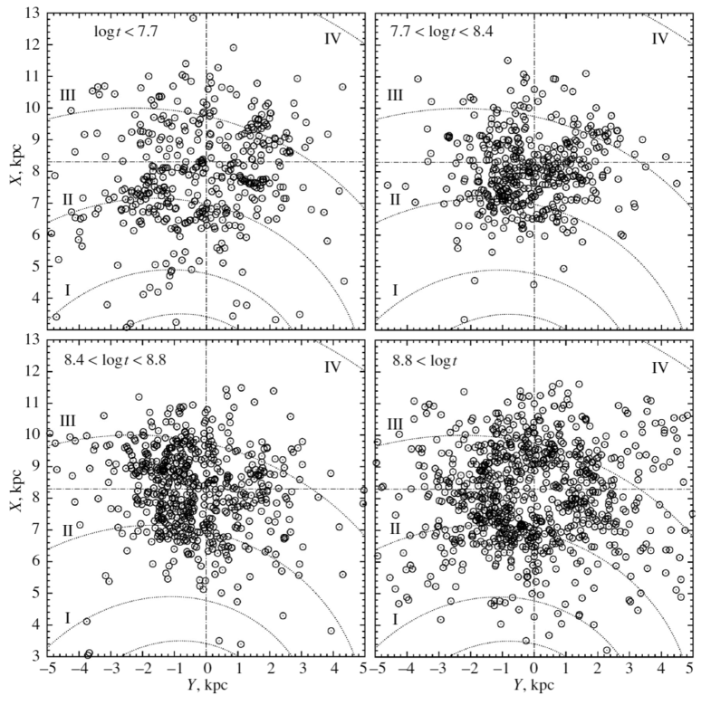
Figure 1: Distribution of four samples of OSCs with different ages on the Galactic $XY$ plane. The Sun’s coordinates are $(X,Y)=(8.3,0)$ kpc. The four-armed spiral pattern with the pitch angle $i=-13^{\circ}$ found from masers (Bobylev and Bajkova 2014c) is shown. The spiral arm segments are numbers by Roman numerals.

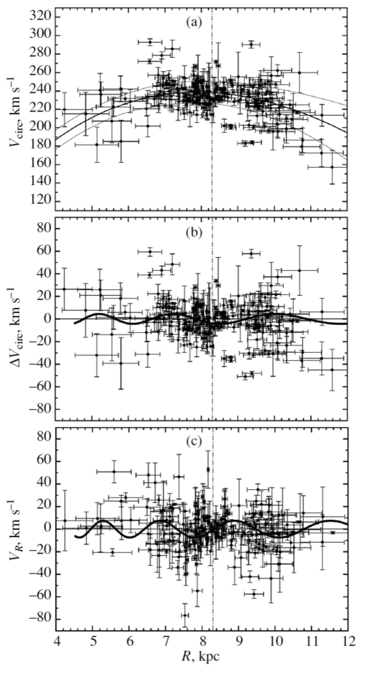
Figure 2: (a) Galactic rotation curve constructed from the sample of 209 youngest OSCs $(\log t<7.7)$ with an indication of the boundaries of the $1\sigma$ confidence intervals, (b) the residual rotation velocities $\Delta V_{circ}$ of stars, and (c) the radial velocities $V_{R}$ of stars; the vertical dash–dotted line marks the Sun’s position.

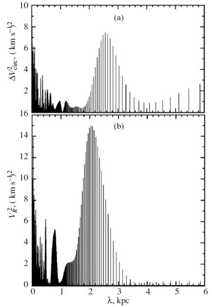
Figure 3: Power spectrum of the residual tangential, $\Delta V_{circ}$ (a), and radial, $V_{R}$ (b), velocities for the sample of 209 youngest $(\log t<7.7)$ OSCs.

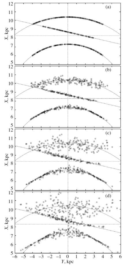
Figure 4: Distributions of 280 model OSCs on the Galactic $XY$ plane (a) obtained by the Monte Carlo method as a result of one realization with the addition of random errors to the distances of 10% (b), 20% (c), and 30% (d).

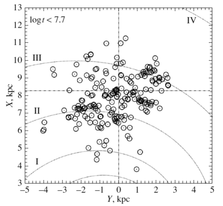
Figure 5: Distributions of the sample of 209 young OSCs with known space velocities on the Galactic $XY$ plane. The Sun’s coordinates are $(X,Y)=(8.3,0)$ kpc. The four-armed spiral pattern with the pitch angle $i=-13^{\circ}$ found from masers (Bobylev and Bajkova 2014c) is shown. The spiral arm segments are numbered by Roman numerals.

On the Geometry of the Spiral Pattern

As can be seen from Fig. 1, the spiral pattern in the distribution of OSCs is visible, but only in the sample of youngest clusters $(\log t<7.7).$ However, there is significant noise even in the distribution of these young OSCs.

We simulated the distribution of young clusters on the Galactic $XY$ plane as a function of errors in their distances. For this purpose we generated a model sample of 280 points corresponding to the clusters populating the Local Arm (100 points) and two more distant segments of the spiral arms, Perseus and Carina–Sagittarius (90 points in each). The Local Arm was represented by a line segment with a total length of 6 kpc that was slightly displaced from the Sun toward the Galactic anticenter and oriented at an angle of $13^{\circ}$ to the $Y$ axis (Bobylev and Bajkova 2014d). In this model the segments of the Perseus ($X\approx 9.5$ kpc) and Carina–Sagittarius ($X\approx 7$ kpc) spiral arms are represented as arcs of circumferences.

We generated three realizations by the Monte Carlo method with the addition of random errors to the distances of 10%, 20%, and 30%. The simulation results are presented in Fig. 4, where the upper panel shows the initial model.

Our simulations showed the following: (i) if the objects lie on the line of sight, as is the case for the edge segments of the Carina.Sagittarius arm (II, $X\approx$7 kpc) and the Local Arm, then the belonging to the specified model is retained even at large random errors in the distances; (ii) from the distribution of objects in the Perseus arm (III, $X\approx$9.5 kpc) that lie on different lines of sight we can draw the conclusion about a fundamental similarity to the distribution of the youngest $(\log t<7.7)$ OSCs (Fig. 1) for a random error level of at least 20%.

Figure 5 presents the distribution of the sample of 209 OSCs with known space velocities on the Galactic $XY$ plane. In comparison with the distribution of the youngest OSCs (Fig. 1), the connection of OSCs with the plotted spiral pattern is seen more clearly here. The Local Arm and part of the Carina–Sagittarius arm are especially prominent. This is probably because the selection of cluster members and the distance determination are made more reliably at known line-of-sight velocities and proper motions.

In Fig. 1 we have more cases where the candidates for clusters were selected based on the proper motions of individual stars with a comparatively low accuracy. This causes the errors in the distance estimates to increase and, consequently, the spiral pattern to be blurred. The motion of such clusters more likely reflects the kinematics of the Galactic “background” than the clusters themselves. However, such a smoothing effect is more likely useful than harmful in determining the Galactic rotation parameters.

The cluster age is also important. For example, Dias and Lépine (2005) showed that OSCs with an age of no more than 20 Myr are closely connected with the spiral structure.

DISCUSSION

At present, there is a sample of more than 120 maser sources whose trigonometric parallaxes were measured by the VLBI technique with a high accuracy, with a mean error of $\pm$20 mas and, some of them, with a record error of $\pm$5 mas. Honma et al. (2012) estimated the Sun’s velocity $V_{0}=238\pm 14$ km s^-1 (for the derived $R_{0}=8.05\pm 0.45$ kpc) from their analysis of masers, Reid et al. (2014) determined $V_{0}=240\pm 8$ km s^-1 (for the derived $R_{0}=8.34\pm 0.16$ kpc), and, finally, Bobylev and Bajkova (2014a) calculated $V_{0}=241\pm 7$ km s^-1 (for the adopted $R_{0}=8.3\pm 0.2$ kpc). It can be seen that the value of this velocity $V_{0}=236\pm 6$ km s^-1 (for $R_{0}=8.3\pm 0.2$ kpc) found from a large amount of data on OSCs in solution (15) is in good agreement with the present-day estimates obtained in other works.

We detected the influence of the spiral structure only in the spatial distribution and kinematics of the youngest clusters whose age does not exceed 50 Myr. It is interesting to compare the parameters found from these clusters, such as the velocity perturbation amplitudes $f_{\theta},$ and $f_{R},$ the wavelengths $\lambda_{\theta},$ and $\lambda_{R},$ and the Sun’s phases in the spiral density wave $(\chi_{\odot})_{\theta},(\chi_{\odot})_{R},$ with those determined from other samples.

For example, Bobylev and Bajkova (2015a) analyzed spectroscopic binaries and OB3 stars with the calcium distance scale based on a spectral analysis. Based on a sample of spectroscopic binaries, we found the following parameters for the model of a four-armed spiral pattern $(m=4,R_{0}=8$ kpc): $f_{R}=9.5\pm 1.5$ km s^-1 and $f_{\theta}=3.2\pm 1.4$ km s^-1, $\lambda_{R}=2.8\pm 0.5$ kpc $(i_{R}=-13^{\circ}\pm 4^{\circ})$ at the Sun’s phase in the spiral density wave $(\chi_{\odot})_{R}=-95^{\circ}\pm 15^{\circ},$ $\lambda_{\theta}=2.6\pm 0.4$ kpc $(i_{\theta}=-12^{\circ}\pm 3^{\circ})$ at $(\chi_{\odot})_{\theta}=-93^{\circ}\pm 12^{\circ}.$ We obtained the following estimates from a sample of OB3 stars with the calcium distance scale: $f_{R}=11.8\pm 1.3$ km s^-1 and $\lambda_{R}=2.1\pm 0.3$ kpc $(i_{R}=-9.5^{\circ}\pm 1.7^{\circ})$ at the Sun’s phase in the spiral density wave $(\chi_{\odot})_{R}=-86^{\circ}\pm 7^{\circ}.$

Zabolotskikh et al. (2002) obtained $f_{\theta}=0.4\pm 2.3$ km s^-1, $f_{R}=6.6\pm 2.5$ km s^-1, $i=-6.6^{\circ}\pm 0.9^{\circ}$ and $\chi_{\odot}=-97^{\circ}\pm 18^{\circ}$ $(m=2,R_{0}=7.5$ kpc) from a sample of blue supergiants and $f_{\theta}=0.2\pm 1.6$ km s^-1, $f_{R}=5.5\pm 2.3$ km s^-1, $i=-12.2^{\circ}\pm 0.7^{\circ}$ and $\chi_{\odot}=-88^{\circ}\pm 14^{\circ}$ $(m=4,R_{0}=7.5$ kpc) from a sample of open clusters. Note that Zabolotskikh et al. (2002) determined the parameters of the spiral density wave simultaneously with the Galactic rotation parameters, i.e., no spectral analysis was used. Dambis et al. (2015) found the phase $\chi_{\odot}=-121^{\circ}\pm 3^{\circ}$ $(m=4,R_{0}=7.1$ kpc) by analyzing the currently most complete kinematic sample of classical Cepheids. Using a sample of 107 masers with measured trigonometric parallaxes and based on a spectral analysis, Bobylev and Bajkova (2015b) estimated $f_{\theta}=6.0\pm 2.6$ km s^-1 and $f_{R}=7.2\pm 2.2$ km s^-1, $\lambda_{\theta}=3.2\pm 0.5$ kpc and $\lambda_{R}=3.0\pm 0.6$ kpc $(m=4,R_{0}=8.0$ kpc), $(\chi_{\odot})_{\theta}=-79^{\circ}\pm 14^{\circ}$ and $(\chi_{\odot})_{R}=-199^{\circ}\pm 16^{\circ}$.

We can see that the wavelengths $\lambda_{\theta},$ $\lambda_{R}$ and the Sun’s phases in the spiral density wave $(\chi_{\odot})_{\theta},$ $(\chi_{\odot})_{R}$ found in this paper from clusters are in good agreement with the results of the analysis of OB stars, Cepheids, and masers. The fairly large amplitude of the perturbations in the tangential velocities of OSCs $f_{\theta}=5.6\pm 1.6$ km s^-1, which from samples of OB stars usually turns out to be no significantly different from zero, is of considerable interest.

The connection of the spatial distribution of young OSCs with the spiral structure was pointed out by many authors (Dias and Lépine 2005; Naoz and Shaviv 2007; Loktin and Popova 2007; Griv et al. 2014). Since the radius of the sample with reliable OSC distance estimates is small (approximately 3.5 kpc), the estimates of the parameters of the spiral structure based on OSCs are unreliable. For example, from their analysis of OSCs Popova and Loktin (2005) found the pitch angle $i=-21.5^{\circ}$, while based on a joint analysis of OSCs, HII clouds, and Cepheids these authors hypothesized the existence of a 12-armed spiral structure in the Galaxy (Loktin and Popova 2007).

Hou and Han (2014) gave an overview of the present-day estimates for the parameters of the spiral structure obtained from objects (HI clouds, HII regions, molecular clouds, and masers) distributed over the entire Galaxy. These authors justify the four-armed model with a pitch angle close to $-13^{\circ}.$ Based on a sample of 565 classical Cepheids, Dambis et al. (2015) found the pitch angle $i=-9.5^{\circ}\pm 0.1^{\circ}$ within the four-armed model of the spiral structure. According to the latest estimate by Valleé (2015) obtained by analyzing various indicators, the pitch angle of the four-armed spiral pattern in the Galaxy is $i=-13.1^{\circ}\pm 0.6^{\circ}.$

CONCLUSIONS

The Galactic rotation parameters were redetermined using a large sample of open star clusters from the MWSC (Milky Way Star Clusters) catalogue produced by Kharchenko et al. (2013). An important advantage of the catalogue is the homogeneity of its proper motions that were obtained using the PPMXL catalogue (Röser et al. 2010).

The circular rotation velocity of the solar neighborhood around the Galactic center was found from data on $\sim$2000 OSCs to be $V_{0}=236\pm 6$ km s^-1 for the adopted Galactocentric distance of the Sun $R_{0}=8.3\pm 0.2$ kpc. The Oort constants $A=-14.52\pm 0.32$ km s^-1 kpc^-1 and $B=13.95\pm 0.48$ km s^-1 kpc^-1 found in this solution show that the Galactic rotation curve is nearly flat in the solar neighborhood. This solution was obtained using almost all clusters from the catalogue, because they are all provided with the proper motions. In addition, the line-of-sight velocities of the clusters were also involved in the solution.

Remarkably, the Galactic rotation parameters ($\Omega_{0},$ $\Omega^{\prime}_{0},$ $\Omega^{\prime\prime}_{0},$ $V_{0}$, $A,$ $B$) that were determined from samples of clusters with various ages are very stable. In addition, the values of $\Omega_{0},$ $V_{0}$, $A,$ and $B$ are close to those found by various authors from masers with measured trigonometric parallaxes. Obviously, this favorably characterizes the system of proper motions of the PPMXL catalogue.

The parameters of the Galactic spiral density wave satisfying the linear Lin.Shu model were found from the series of residual tangential, $\Delta V_{circ},$ and radial, $V_{R},$ velocities for the sample of youngest clusters $(\log t<7.7)$ using a periodogram analysis. The amplitudes of the tangential and radial velocity perturbations are $f_{\theta}=5.6\pm 1.6$ km s^-1 and $f_{R}=7.7\pm 1.4$ km s^-1, respectively; the perturbation wavelengths are $\lambda_{\theta}=2.6\pm 0.5$ kpc ($i_{\theta}=-11^{\circ}\pm 2^{\circ}$) and $\lambda_{R}=2.1\pm 0.5$ kpc ($i_{R}=-9^{\circ}\pm 2^{\circ}$) for the adopted four-armed model of the spiral pattern $(m=4).$ The Sun’s phase in the spiral density wave is $(\chi_{\odot})_{\theta}=-62^{\circ}\pm 9^{\circ}$ and $(\chi_{\odot})_{R}=-85^{\circ}\pm 10^{\circ}$ from the residual tangential and radial velocities, respectively. No influence of the spiral structure in the velocities and positions of older clusters $(\log t>7.7)$ was detected.

Monte Carlo simulations of the distribution of clusters in space showed the errors in the distances to be, on average, no less than 20%.

ACKNOWLEDGMENTS

We are grateful to the referees for their helpful remarks that contributed to an improvement of this paper. This work was supported by the “Transitional and Explosive Processes in Astrophysics” Program P–41 of the Presidium of Russian Academy of Sciences.

REFERENCES

1. L.H. Amaral and J.R.D. Lépine, Mon. Not. R. Astron. Soc. 286, 885 (1997).

2. A.T. Bajkova and V.V. Bobylev, Astron. Lett. 38, 549 (2012).

3. A.T. Bajkova and V.V. Bobylev, Baltic Astron. 24, 43 (2015).

4. V.V. Bobylev, A.T. Bajkova, and S.V. Lebedeva, Astron. Lett. 33, 720 (2007).

5. V.V. Bobylev, A.T. Bajkova, and A.S. Stepanishchev, Astron. Lett. 34, 515 (2008).

6. V.V. Bobylev and A.T. Bajkova, Astron. Lett. 38, 638 (2012).

7. V.V. Bobylev and A.T. Bajkova, Astron. Lett. 39, 532 (2013).

8. V.V. Bobylev and A.T. Bajkova, Astron. Lett. 40, 389 (2014a).

9. V.V. Bobylev and A.T. Bajkova, Astron. Lett. 40, 773 (2014b).

10. V.V. Bobylev and A.T. Bajkova, Mon. Not. R. Astron. Soc. 437, 1549 (2014c).

11. V.V. Bobylev and A.T. Bajkova, Astron. Lett. 40, 783 (2014c).

12. V.V. Bobylev and A.T. Bajkova, Astron. Lett. 41, 473 (2015a).

13. V.V. Bobylev and A.T. Bajkova, Mon. Not. R. Astron. Soc. 447, L50 (2015b).

14. C. Bonatto, L.O. Kerber, E. Bica, and B.X. Santiago, Astron. Astrophys. 446, 121 (2006).

15. J. Borissova, A.-N. Chené, S. Ramirez Alegria, S. Sharma, J.R.A. Clarke, R. Kurtev, I. Negueruela, A. Marco, P. Amigo, et al., Astron. Astrophys. 569, A24 (2014).

16. D. Camargo, C. Bonatto, and E. Bica, Mon. Not. R. Astron. Soc. 450, 4150 (2015).

17. D. Camargo, E. Bica, and C. Bonatto, Mon. Not. R. Astron. Soc. 455, 3126 (2016).

18. B. Chaboyer, E.M. Green, and J. Liebert, Astron. J. 117, 1360 (1999).

19. L. Chen, J.L. Hou, and J.J. Wang, Astron. J. 125, 1397 (2003).

20. G.C. Clayton and E.L. Fitzpatrick, Astron. J. 93, 157 (1987).

21. N.J.G. Cross, R.S. Collins, R.G. Mann, M.A. Read, E.T.W. Sutorius, R.P. Blake, M. Holliman, N.C. Hambly, et al., Astron. Astrophys. 548, A119 (2012).

22. A.K. Dambis, L.N. Berdnikov, Yu.N. Efremov, A.Yu. Knyazev, A.S. Rastorguev, E.V. Glushkova, V.V. Kravtsov, D.G. Terner, D.D. Madzhess, and R. Sefako, Astron. Lett. 41, 489 (2015).

23. W.S. Dias, B.S. Alessi, A. Moitinho, and J.R.D. Lépine, Astron. Astrophys. 389, 871 (2002).

24. W.S. Dias and J.R.D. Lépine, Astrophys. J. 629, 825 (2005).

25. P. Fedorov, A. Myznikov, and V. Akhmetov, Mon. Not. R. Astron. Soc. 393, 133 (2009).

26. P. Fedorov, V. Akhmetov, and V.V. Bobylev, Mon. Not. R. Astron. Soc. 416, 403 (2011).

27. E.D. Friel, Ann. Rev. Astron. Astrophys. 33, 381 (1995).

28. D. Froebrich, A. Scholz, and C.L. Raftery, Mon. Not. R. Astron. Soc. 374, 399 (2007).

29. S. Gillessen, F. Eisenhauer, T.K. Fritz, H. Bartko, K. Dodds-Eden, O. Pfuhl, T. Ott, and R. Genzel, Astroph. J. 707, L114 (2009).

30. E.V. Glushkova, A.K. Dambis, A.M. Mel’nik, and A.S. Rastorguev, Astron. Astrophys. 329, 514 (1998).

31. E.V. Glushkova, S.E. Koposov, I.Yu. Zolotukhin, Yu.V. Beletskii, A.D. Vlasov, and S.I. Leonova, Astron. Lett. 36, 75 (2010).

32. E. Griv, C.-C. Lin, C.-C. Ngeow, and I.G. Jiang, New Astron. 29, 9 (2014).

33. The HIPPARCOS and Tycho Catalogues, ESA SP–1200 (1997).

34. M. Honma, T. Nagayama, K. Ando, T. Bushimata, Y.K. Choi, T. Handa, T. Hirota, H. Imai, T. Jike, et al., Publ. Astron. Soc. Jpn. 64, 136 (2012).

35. L.G. Hou and J.L. Han, Astron. Astrophys. 569, A125 (2014).

36. Y.C. Joshi, Mon. Not. R. Astron. Soc. 362, 1259 (2005).

37. Y.C. Joshi, Mon. Not. R. Astron. Soc. 378, 768 (2007).

38. T.C. Junqueira, C. Chiappini, J.R.D. Lépine, I. Minchev, and B.X. Santiago, Mon. Not. R. Astron. Soc. 449, 2336 (2015).

39. N.V. Kharchenko and S. Röser, Kinem. Phys. Celest. Bodies 17, 409 (2001).

40. N.V. Kharchenko, A.E. Piskunov, S. Röser, E. Schilbach, and R.-D. Scholz, Astron. Astrophys. 438, 1163 (2005a).

41. N.V. Kharchenko, A.E. Piskunov, S. Röser, E. Schilbach, and R.-D. Scholz, Astron. Astrophys. 440, 403 (2005b).

42. N.V. Kharchenko, R.-D. Scholz, A.E. Piskunov, S. Röser, and E. Schilbach, Astron. Nachr. 328, 889 (2007).

43. N.V. Kharchenko, A.E. Piskunov, S. Roeser, E. Schilbach, and R.-D. Scholz, Astron. Astrophys. 558, 53 (2013).

44. S. Koposov, E. Glushkova, and I. Zolotukhin, Astron. Nachr. 326, 597 (2005).

45. S.E. Koposov, E.V. Glushkova, and I.Yu. Zolotukhin, Astron. Astrophys. 486, 771 (2008).

46. J.R.D. Lépine, W.S. Dias, and Yu. Mishurov, Mon. Not. R. Astron. Soc. 386, 2081 (2008).

47. C.C. Lin and F.H. Shu, Astrophys. J. 140, 646 (1964).

48. A.V. Loktin and G.V. Beshenov, Astron. Rep. 47, 6 (2003).

49. A.V. Loktin and M.E. Popova, Astron. Rep. 51, 364 (2007).

50. A. Maeder and J.C. Mermilliod, Astron. Astrophys. 93, 136 (1981).

51. P.G.P. Moroni and O. Straniero, Astrophys. J. 581, 585 (2002).

52. S. Naoz and N.J. Shaviv, New Astron. 12, 410 (2007).

53. M. Netopil, E. Paunzen, U. Heiter, and C. Soubiran, Astron. Astrophys. 585, 150 (2016).

54. R.L. Phelps, Astrophys. J. 483, 826 (1997).

55. A.E. Piskunov, N.V. Kharchenko, S. Röser, E. Schilbach, and R.-D. Scholz, Astron. Astrophys. 445, 545 (2006).

56. M.E. Popova and A.V. Loktin, Astron. Lett. 31, 171 (2005).

57. M.J. Reid, K.M. Menten, A. Brunthaler, X.W. Zheng, T.M. Dame, Y. Xu, Y. Wu, B. Zhang, et al., Astrophys. J. 783, 130 (2014).

58. S. Röser, M. Demleitner, and E. Schilbach, Astron. J. 139, 2440 (2010).

59. S. Schmeja, N.V. Kharchenko, A.E. Piskunov, S. Röser, E. Schilbach, D. Froebrich, and R.-D. Scholz, Astron. Astrophys. 568, A51 (2014).

60. R.-D. Scholz, N.V. Kharchenko, A.E. Piskunov, S.Röser, and E. Schilbach, Astron. Astrophys. 581, A39 (2015).

61. M.F. Skrutskie, R. M. Cutri, R. Stiening, M.D. Weinberg, S. Schneider, J.M. Carpenter, C. Beichman, R. Capps, et al., Astron. J. 131, 1163 (2006).

62. R.J. Trumpler, Publ. Astron. Soc. Pacif. 42, 214 (1930).

63. B.A. Twarog and B.J. Anthony-Twarog, Astron. J. 97, 759 (1989).

64. J.P. Vallée, Mon. Not. R. Astron. Soc. 450, 4277 (2015).

65. E.L. Wright, P.R.M. Eisenhardt, A.K. Mainzer, M.E. Ressler, R.M. Cutri, T. Jarrett, J.D. Kirkpatrick, D. Padgett, et al., Astron. J. 140, 1868 (2010).

66. M.V. Zabolotskikh, A.S. Rastorguev, and A.K. Dambis, Astron. Lett. 28, 454 (2002).