Random-phase-approximation theory for sequence-dependent, biologically functional liquid-liquid phase separation of intrinsically disordered proteins

Abstract

Intrinsically disordered proteins (IDPs) are typically low in nonpolar/hydrophobic but relatively high in polar, charged, and aromatic amino acid compositions. Some IDPs undergo liquid-liquid phase separation in the aqueous milieu of the living cell. The resulting phase with enhanced IDP concentration can function as a major component of membraneless organelles that, by creating their own IDP-rich microenvironments, stimulate critical biological functions. IDP phase behaviors are governed by their amino acid sequences. To make progress in understanding this sequence-phase relationship, we report further advances in a recently introduced application of random-phase-approximation (RPA) heteropolymer theory to account for sequence-specific electrostatics in IDP phase separation. Here we examine computed variations in phase behavior with respect to block length and charge density of model polyampholytes of alternating equal-length charge blocks to gain insight into trends observed in IDP phase separation. As a real-life example, the theory is applied to rationalize/predict binodal and spinodal phase behaviors of the 236-residue N-terminal disordered region of RNA helicase Ddx4 and its charge-scrambled mutant for which experimental data are available. Fundamental differences are noted between the phase diagrams predicted by RPA and those predicted by mean-field Flory-Huggins and Overbeek-Voorn/Debye-Hückel theories. In the RPA context, a physically plausible dependence of relative permittivity on protein concentration can produce a cooperative effect in favor of IDP-IDP attraction and thus a significant increased tendency to phase separate. Ramifications of these findings for future development of IDP phase separation theory are discussed.

1 Introduction

Globular proteins have been the predominant focus of structural biology since the folded myoglobin structure was revealed by X-ray crystallography in 1958 [1]. However, while many proteins need to fold to a relatively fixed structure for biological activity, it is now clear — after more than one and a half decade of intense research [2, 3, 4, 5, 6] — that intrinsically disordered proteins (IDPs) perform key functions in cellular processes [7, 8, 9, 10, 11, 12, 13, 14, 15, 16]. This advance led to the recognition that different biological functions can be bestowed upon protein conformations of various degrees of flexibility [8]. Many IDPs do “fold” or become otherwise ordered upon binding to their folded partners [6]. Recently, an IDP was found to fold by phosphorylation as a regulatory switch [17]. But IDPs can also form “fuzzy complexes” [18], i.e., they remain largely disordered even when they are functionally bound, as exemplified by the interaction between the IDP cyclin dependent kinase inhibitor Sic1 and the ubiquitin ligase SCF^Cdc4 [19, 20, 21]. Although IDP conformations are largely disordered, their ensemble distributions are not random. Like globular proteins, their behaviors are governed by their amino acid sequences [13]. In this respect, functional IDPs entail a type of biomolecular self-organization that is perhaps even more challenging to comprehend physico-chemically than the self-assembly of globular proteins.

More recently, a previously unexpected function of IDPs was discovered. Some IDPs have been found to be the main constituents of functional membraneless organelles in the living cell, the assembly and disassembly of which is apparently underpinned by liquid-liquid IDP phase separation [22, 23, 24, 25, 26, 27, 28, 29, 30, 31, 32, 33, 34, 35, 36]. Such IDP phase behaviors are sequence-dependent [30, 36] and may be regulated posttranslationally such as by phosphorylation of germ plasm component proteins in P granules [29] and by arginine methylation of Ddx4^N1 organelles [30]. Droplets of these IDP-rich phase are fundamentally different from amyloids [37, 16] and condensed phases of folded globular proteins [38, 39, 40, 41, 42, 43, 44]. Membraneless organelles include nuceloli, Cajal bodies, and stress granules. They are a form of cell compartmentalization, creating their peculiar microenvironments [34, 35] that play critical roles in cellular integrity, homeostasis, gene regulation and the cell cycle. Examples include the RNA and protein-rich P granules in the germ cell of Caenorhabditis elegans [22, 29] and the RNA-protein (RNP) stress granules induced by exposing human (HeLa) cells to arsenate [32]. Because of the central role of membraneless organelles in cell cycle regulation and thus the disease process of cancer, and that RNP aggregates are often associated with neurodegenerative diseases, a better understanding of the biophysics of IDP phase separation is not only of fundamental biological interest but also of tremendous medical relevance.

Unlike globular proteins, the role of hydrophobic interactions [45] are significantly less dominant in IDPs, which generally contains fewer nonpolar but more polar, charged, and aromatic residues than globular proteins ([46, 47, 48] and references therein). Many IDPs may be regarded as polyampholytes — heteropolymers with both positively and negatively charged monomer units [49, 50]. Dimensions of individual IDP molecules are affected not only by their total charges [51] but also sequence arrangement of charges [52]; their response to denaturant is different from that of unfolded globular proteins [53]. Liquid-liquid phase separation of IDPs is sensitive to the charge pattern along their chain sequences as well [54]. This is evident from recent experiments on the DEAD-box RNA helicase Ddx4 [30] and the Nephrin intracellular domain [36] showing different phase behaviors from their respective charge-scrambled mutants [30, 36]. These behaviors may in principle be addressed by explicit-chain simulations [55]. For computational tractability as well as conceptual advances, however, it is useful to develop an analytical theory of polymer solutions for IDP phase behaviors, notwithstanding the approximate and simplistic nature of all analytical theories of complex systems [43]. In view of the experimental observations, a desirable feature of such theories is to afford an account of sequence-dependent long-range electrostatic interactions that goes beyond classical Flory-Huggins (FH) theory [56, 57, 58], as the latter is strictly speaking only suited for short-range, contact-like interactions such as those arising from hydrophobicity [59].

A variety of analytical theories for electrolytes and charged polymers have been put forth during the last nearly one century since the 1923 publication of the Debye-Hückel (DH) theory that accounts for the nonideality of electrolyte solutions [60]. DH theory, or equivalently the linearized Poisson-Boltzmann (PB) equation, has been applied to electrolyte and polyelectrolyte systems with identical or nonidentical ions [61, 62]. The PB equation has since been augmented, e.g., by incorporating van der Waals forces, to construct more enriched theories such as that of Derjaguin, Landau, Verwey, and Overbeek (DLVO theory, 1941, 1948) to rationalize the stability of lyophobic (solvent averting) colloid [63, 64]. Subsequently, theories that go beyond the mean-field PB equation such as the closure relations to solve the Wertheim-Ornstein-Zernike (WOZ) equation [65, 66, 62], e.g. the hypernetted-chain/mean-spherical approximation (HNC/MSA) ([67] and references therein) and the Percus-Yevick approximation [68], as well as the random phase approximation (RPA) [69, 70], were devised to model various electrolyte systems, including globular polyions as well as flexible polyelectrolytes and polyampholytes [66, 71, 62, 72, 73, 74, 75, 76].

Although the main concern of many of these theories has been uniformly charged polyelectrolytes, the charge pattern on flexible polyampholytes has not escaped recognition as having a significant impact on the conformational distribution of individual chains as well as multiple-chain phase properties [49, 50]. Based on beyond-DH formulations that take into account chain connectivity, theories such as RPA [77, 73, 78] and HNC/MSA [75, 76, 79] have been applied to study polyampholyte systems. However, such effort has not been widely pursued, likely because of a lack of experimental impetus. In the absence of a chemical process comparable to the cellular apparatus capable of synthesizing specific amino acid sequences accurately, synthesis of nonbiological polyampholytes with specific sequences is extremely difficult if not impossible. In such synthesis, often only the initial conditions can be controlled, resulting in a polymerization process that can only be monitored at the level of thermal average [50]. Consequently, research on nonbiological polyampholytes has focused on either the ensemble average of all possible random sequences [49, 77, 78] or simple block polyampholytes with a strictly alternating [77], diblock [73], or four-block charge patterns [80, 79].

As far as charge effects in biomolecules are concerned, the Overbeek-Voorn (OV, 1957) theory [81] is a rudimentary approach that combines DH theory with FH conformational entropy [58, 69]. OV theory has been applied to rationalize behavior of various complex coacervations, e.g. between albumin and acacia [82] as well as between whey proteins and gum arabic [83, 84]. Beyond-mean-field theories have also been applied to model phase separation of folded globular proteins in aqueous solutions, wherein protein molecules are treated as spheres with no or few internal degrees of freedom, similar to the idealized folded states in earlier mean-field models for electrostatic effects in protein folding and stability [85, 86]. These include, but are not limited to, RPA [38], perturbation theories [39, 40] and, notably, a recent application Wertheim’s thermodynamic perturbation theory (TPT1) [87] by Vlachy and coworkers to rationalize protein aggregation induced by salt as well as the liquid-liquid co-existence curve of folded lysozyme and $\gamma$ IIIa-crystallin solutions [44]. One of the goals of these studies has been to better understand crystallization of globular proteins for X-ray crystallography, including under harsh conditions with non-physiological pH and salt concentrations [88]. Effects of specific amino acid sequences were not considered in these approaches.

The recent discovery of biologically functional IDPs as individual molecules and also collectively via phase-separation has sparked a renewed interest in polymer solution theories [27, 33, 89, 90]. For instance, Sawle and Ghosh developed an analytical formulation to account for sequence-specific electrostatic effects on the dimension of individual polyampholytes [89], providing predictions consistent with prior atomic simulation results [52]. In this context, we recently outlined an approach to apply RPA theory to model sequence-specific long-range electrostatic effects in IDP phase separation [91]. Compared to the mean-field FH [26, 27, 30], DH and OV [33] theories that have been applied or advocated for the study of IDP phase separation, our approach has the advantage of treating chain connectivity rather explicitly and hence it allows for a direct, unambiguous input of the charge pattern along the chain sequence into the theory [70, 73, 74]. The approach has been applied to the 236-residue IDP fragment Ddx4^N1 of Ddx4, a protein required for the assembly and maintenance of membraneless organelles that are essential for germ cell development in mammals, worms and flies [30, 92]. Our theory is successful in rationalizing the experimentally observed salt-dependent phase separation of Ddx4^N1 as well as the drastically different phase behaviors of Ddx4^N1 and a charge scrambled mutant Ddx4^N1CS [91]. The new results reported below are further development of this theory, including detailed comparisons with mean-field FH and OV/DH approaches, and exploration of extensions of the theory that may provide deeper physical insights into the fascinating phenomenon of biologically functional IDP liquid-liquid phase separation in general.

2 A sequence-specific RPA theory for polypeptide charge patterns

As described recently [91], our theory is for aqueous solutions of neutral or nearly-neutral polyampholytes such as Ddx4^N1 with small monovalent counterions and salt, and is based on previous RPA methods [77, 73]. (For simplicity of notation, Ddx4^N1 and its mutant are sometimes referred to simply as “Ddx4” in the discussion below when the meaning is obvious from the context). Each polyampholyte chain is composed of $N$ amino acid residues (monomers) with charges $\{\sigma_{i}\}=\{\sigma_{1},\sigma_{2},\dots,\sigma_{N}\}$ given in units of the electronic charge $e$ ($\sigma_{i}=\pm 1$ or $0$). Using the same notation as in [91], $\rho_{m}$, $\rho_{c}$, and $\rho_{s}$ are, respectively, the average number densities of the monomers of the polyampholytes, counterions, and salt in a total solution volume $V$, where $\rho_{c}=\rho_{m}\left|\sum_{i}\sigma_{i}\right|/N$ because the number of counterions is equal to the total net charge of polyampholytes.

A major part of the configurational entropy of the system is based on the FH lattice model [58, 69], in which spatial volume is partitioned into lattice sites each with a volume $a^{3}$, which is of order of an individual solvent molecule; thus the total number of lattice sites is $M=V/a^{3}$. The total free energy $F$ per lattice site in units of $k_{\rm B}T$ is given by

$$f\equiv\frac{Fa^{3}}{Vk_{\rm B}T}=-s+f_{\rm int},$$ (1)

where $k_{\rm B}$ is Boltzmann’s constant and $T$ is absolute temperature, $-s$ is the entropic contribution to free energy from FH consideration, and $f_{\rm int}$ accounts for the effective solvent-mediated interactions in the system. The $f_{\rm int}$ term is modeled under an RPA framework [91], which provides a beyond-mean-field, approximate account of local density fluctuations. RPA may be applied to any form of two-body interactions in principle. In this paper, however, we are interested in situations of polyampholyte phase separation where electrostatics is the dominant enthalpic contribution. Although $f_{\rm int}$ is often characterized as “enthalpic” for terminological simplicity [91], it is useful to keep in mind that effective solvent-mediated interactions such as hydrophobicity can be temperature dependent [93] and therefore contain entropic contributions. As will be discussed below, the present RPA form of $f_{\rm int}$ also contains entropic contributions from chain connectivity.

2.1 Entropy in a size-dependent mean-field lattice model

Most formulations of FH  [58], including recent applications to IDP phase separation [30, 91], assume for simplicity that a solvent molecule is of the same size of a monomer of the polymer of interest, each occupying a single lattice site. Numerical results presented in this paper were obtained using the same assumption. However, it is useful for future development of theory to consider here a generalization of the FH approach that is capable of accounting for solvent, monomers, salt ions, and counterions of different sizes. Based on a detailed consideration of the physical meaning of the entropy term in the FH formulation [94] (especially discussion relating to Figs. 4 and 5 in this reference), a generalized FH configurational entropy of a collection of $m$ different types of polymers labeled by $i$ $=1,2,\dots,m$, each with $N_{i}$ monomers of size $r_{i}a^{3}$ — where individual solvent molecules, counterion and salt ions are regarded as special cases of polymers with $N_{i}=1$ — may be derived as follows. (Note that the meaning of index $i$ here is different from that in some other parts of the paper where it is used to label the monomers along a polymer. The meaning of “dummy” summation indices should always be clear from the context nonetheless.) Without loss of generality, a value of $a^{3}$ can always be chosen such that all $r_{i}$’s are integers or as close to being so as desired. In such a system, the total number of lattice sites is given by

$$M=\frac{V}{a^{3}}=\sum_{i=1}^{m}r_{i}n_{i}N_{i}.$$ (2)

where $n_{i}$ is the number of type-$i$ polymer molecules in the solution. We may now define the number density of type-$i$ monomer in units of $1/a^{3}$ as

$$\phi_{i}=\rho_{i}a^{3}=\frac{n_{i}N_{i}}{M},$$ (3)

which allows rewriting Eq. (2) as

$$\sum_{i=1}^{m}r_{i}\phi_{i}=1.$$ (4)

Note that $\phi_{i}$ is not the volume fraction [91] when $r_{i}\neq 1$.

Following the argument in the original derivation of FH [58], we separate configurational entropy $S=k_{B}\ln\Omega$ into a term arising from the translational freedom of the first monomer (or center of mass) of each polymer ($\Omega_{\rm CM}$) and another term accounting for the conformational freedom of each polymer with a fixed position for the first monomer or center of mass ($\Omega_{\rm conf}$) such that $\Omega=\Omega_{\rm CM}\Omega_{\rm conf}$. The translational term corresponds to the number of ways of arranging $\sum_{i}n_{i}$ monomers each being the first monomer of a polymer, which equals

$$\Omega_{\rm CM}=\frac{M!}{(M-\sum_{i=1}^{m}n_{i})!\prod_{i=1}^{m}n_{i}!}$$ (5)

when all $r_{i}=1$. As for the conformational term, we first recall the standard derivation for the case of $r_{i}=1$ for all $i$ on a lattice with $z$ nearest neighboring sites for each lattice site. The decreasing probability of inserting an additional monomer without violating excluded volume, as the lattice is filled, is taken into account in a mean-field manner:

$$\Omega_{\rm conf} =(z-1)^{{\cal N}_{1}}\prod_{l=0}^{{\cal N}_{2}-1}\left(1-\frac{\sum_{i=1}^{m}n_{i}+l}{M}\right)$$ (6)

$$=\frac{(z-1)^{{\cal N}_{1}}}{M^{{\cal N}_{2}}}\left(M-\sum_{i=1}^{m}n_{i}\right)!\;,$$

where ${\cal N}_{1}={\cal N}_{2}=\sum_{i}n_{i}(N_{i}-1)$ is the total number of lattice sites (monomers) to be inserted after the position of the first monomer of each polymer has been fixed by the procedure described by Eq. (5).

In the generalized system with different $r_{i}$’s, each monomer in a type-$i$ polymer consists of $r_{i}$ lattice sites and is here assumed to have no internal degrees of freedom [94]. The placement of each of these monomers on the lattice may be seen as a series of successive attempted occupation of $r_{i}$ neighboring lattice sites in a unique order (hence no $z-1$ factor) that is consistent with the shape of the monomer and without violation of excluded volume.

In order to account for the possible violation of excluded volume when the second and other lattice sites representing the first monomer of each polymer (when $r_{i}>1$) are placed after the first site has been positioned via the process described in Eq. (5), the expression needs to be modified:

$$\Omega_{\rm CM} \rightarrow\left[\prod_{l=0}^{\sum_{i=1}^{m}n_{i}(r_{i}-1)-1}\left(1-\frac{\sum_{i=1}^{m}n_{i}+l}{M}\right)\right]\Omega_{\rm CM}$$ (7)

$$=\frac{(M-\sum_{i=1}^{m}n_{i})!}{(M-\sum_{i=1}^{m}n_{i}r_{i})!M^{\sum_{i=1}^{m}n_{i}(r_{i}-1)}}\Omega_{\rm CM}\;.$$

The same consideration implies that the total number of lattice sites ${\cal N}_{2}$ to be filled in for the process described by $\Omega_{\rm conf}$ in Eq. (6) is now modified to

$${\cal N}_{2}=\sum_{i=1}^{m}n_{i}(r_{i}N_{i}-1),$$ (8)

with a corresponding modification to Eq. (6):

$$\Omega_{\rm conf}\rightarrow\frac{(z-1)^{\sum_{i=1}^{m}n_{i}(N_{i}-1)}}{M^{\sum_{i=1}^{m}n_{i}r_{i}(N_{i}-1)}}(M-\sum_{i=1}^{m}n_{i}r_{i})!.$$ (9)

By combining Eqs. (5), (7), and (9), we arrive at the expression for the total number of FH microstates for the generalized case:

$$\Omega=\Omega_{\rm CM}\Omega_{\rm conf}=\frac{M!}{\prod_{i=1}^{m}n_{k}!}\frac{(z-1)^{\sum_{i=1}^{m}n_{i}(N_{i}-1)}}{M^{\sum_{i=1}^{m}n_{i}(r_{i}N_{i}-1)}}.$$ (10)

Thus the negative configurational entropy per lattice site

$$-s= -\frac{1}{M}\ln\Omega=\sum_{i=1}^{m}\frac{n_{i}}{M}\ln n_{i}+\text{(terms linear in $n_{i}$)}$$ (11)

$$= \sum_{i=1}^{m}\frac{\phi_{i}}{N_{i}}\ln\phi_{i}+\text{(terms linear in $\phi_{i}$)}$$

is obtained by applying Stirling’s approximation $\ln x!\approx x\ln x-x$ for $x\gg 1$ (in which case the percentage error of omitting the $\ln\sqrt{2\pi x}$ term in the approximation is negligible). It follows that the mixing entropy is given by

$$\Delta s(\{\phi_{i}\})= s(\{\phi_{i}\})\!-\!\sum_{i^{\prime}=1}r_{i^{\prime}}\phi_{i^{\prime}}s(\{\phi_{i^{\prime}}\!=\!1/r_{i^{\prime}},\phi_{i\neq i^{\prime}}\!=\!0\})$$ (12)

$$= \sum_{i=1}^{m}\frac{\phi_{i}}{N_{i}}\ln(\phi_{i}r_{i}).$$

As shown in A, terms of the form $(\phi_{i}/N_{i})\ln r_{i}$ in Eq. (12) that are linear in $\phi_{k}$ have no effect on phase separation. Therefore, for application to phase separation, we may drop these terms and choose the totally demixed configuration as the reference state, then use the mixing entropy expression

$$-s=\frac{\phi_{m}}{N}\ln\phi_{m}+\phi_{c}\ln\phi_{c}+2\phi_{s}\ln\phi_{s}+\phi_{w}\ln\phi_{w}$$ (13)

as the generalized FH entropy term in Eq. (1) for a system of polyampholytes, counterions, and salt. Here $r_{m}$, $r_{c}$, and $r_{s}$, are size factors, respectively, for monomers of the polyampholytes, counterions, and salt ions, $r_{w}$ and $\phi_{w}$ are, respectively, the size factor and number density of water, satisfying

$$r_{w}\phi_{w}=1-r_{m}\phi_{m}-r_{c}\phi_{c}-2r_{s}\phi_{s}$$ (14)

by virtue of Eq. (4).

2.2 RPA treatment of electrostatics

Derivation of RPA electrostatic energy of polyelectrolyte solutions is well documented [70, 74, 95]. We include here for completeness the steps we took to apply RPA to our polyampholyte system, providing some details for the theory we outlined recently [91].

RPA theory neglects all but the trivial zeroth-order and two-body correlation of density fluctuation. Consider a system of different types of monomers (labeled as 1,2,3, …) with densities $\rho^{(1)}({\bf r}),\rho^{(2)}({\bf r}),\rho^{(3)}({\bf r})...$ that are functions of spatial position ${\bf r}$. When the correlation among the densities is accounted for only up to the two-body level, the partition function $Z$ can be expressed as a path integral of all possible density profiles in terms of their Fourier-transformed fluctuations, viz.,

$$Z=\int{\cal D}|\rho_{k}\rangle\exp\left(-\frac{1}{2V}\sum_{k\neq 0}\langle\rho_{-k}|\hat{\cal A}_{k}|\rho_{k}\rangle\right),$$ (15)

where $k$ here is the wave number (for all three dimensions of the reciprocal space of any finite volume $V$), and all variables are Fourier transformed except $V$ which is the total volume of the solution system, appeared here as the normalizing factor for $\sum_{k}$. The matrix $\hat{\cal A}_{k}$ accounts for two-body interactions between arbitrary Fourier transformed densities $\rho_{k}^{(i)}$ and $\rho_{k}^{(j)}$ of monomer types $i$ and $j$; $\hat{\cal A}_{k}$ may correspond to any interaction/correlation that depends only on the relative position ${\bf r}-{\bf r}^{\prime}$ of $\rho({\bf r})$ and $\rho({\bf r}^{\prime})$ in real space. Fourier transformations of density fluctuations are represented by the column vector

$$|\rho_{k}\rangle_{i}\equiv\rho_{k}^{(i)}$$ (16)

and $\langle\rho_{-k}|=(|\rho_{k}\rangle^{*})^{\rm T}$ is the conjugate row vector. The path integral in Eq. (15) is over all monomer types, and over all wave numbers except $k=0$, i.e.,

$${\cal D}|\rho_{k}\rangle=\prod_{i=1}^{m}\prod_{k\neq 0}d\rho_{k}^{(i)}\;.$$ (17)

The $k=0$ term is omitted because

$$\rho_{k=0}^{(i)}=\int d^{3}r\rho^{(i)}(r)=n_{i}$$ (18)

is the total number of type-$i$ monomers, which is a constant that does not contribute to density fluctuation [96].

In the absence of interactions among the monomers, $\hat{\cal A}_{k}$ accounts only for geometric constraints such as chain connectivity, in which case $\hat{\cal A}_{k}$ is the inverse of the bare two-body correlation matrix $\hat{G}_{k}$, viz.,

$${\cal A}_{k}=\hat{G}_{k}^{-1}\;.$$ (19)

This relationship is readily verified by recalling that the two-body correlation is defined by the density conjugate field $h_{k}^{(i)}$ via the partition function

$$Z(|h_{k}\rangle)\!= \int{\cal D}|\rho_{k}\rangle e^{-\sum_{k\neq 0}\left(\frac{1}{2V}\langle\rho_{-k}|\hat{\cal A}_{k}|\rho_{k}\rangle+\langle h_{-k}|\rho_{k}\rangle\right)}$$ (20)

$$= \exp\left(\frac{V}{2}\sum_{k\neq 0}\langle h_{-k}|\hat{\cal A}^{-1}_{k}|h_{k}\rangle\right).$$

The correlation function itself is defined as

$$\langle\rho_{k}^{(i)}\rho_{-k}^{(j)}\rangle=V\left(\hat{G}_{k}\right)_{ij},$$ (21)

where the $V$ factor appears because of translational invariance. Since the correlation function can be determined as the second-order derivative of $\ln Z(|h_{k}\rangle)$,

$$\langle\rho_{k}^{(i)}\rho_{-k}^{(j)}\rangle=\frac{\partial^{2}\ln Z}{\partial h_{k}^{(i)}\partial h_{-k}^{(j)}}\Biggr{|}_{h_{k}^{(i)}=h_{-k}^{(j)}=0}=V\left(\hat{\cal A}^{-1}_{k}\right)_{ij}\;,$$ (22)

Eq. (19) follows from Eqs. (21) and (22).

In our system of polyampholytes and monomeric ions, the matrix elements of $\hat{G}_{k}$ can be classified into four categories: bare monomer-monomer (MM), ion-ion (II), and monomer-ion (MI) correlations with their respective matrices $\hat{G}_{\mathrm{MM}}$, $\hat{G}_{\mathrm{II}}$, $\hat{G}_{\mathrm{MI}}$. Accordingly, $\hat{G}_{k}$ can be arranged as

$$\hat{G}_{k}=\left(\begin{array}[]{cc}\hat{G}_{\mathrm{MM}}(k)&\hat{G}_{\mathrm{MI}}(k)\\ \hat{G}_{\mathrm{IM}}(k)&\hat{G}_{\mathrm{II}}(k)\end{array}\right),$$ (23)

where $\hat{G}_{\mathrm{IM}}=\hat{G}_{\mathrm{MI}}^{\rm T}$. In general, all four correlation submatrices depend on the configurational constraints in the system. For example, crosslinking in polymer gels [97, 95] or ion condensation in charged polymer systems [98] can result in non-trivial correlations. Here we restrict to a simple RPA model of charged polymers and ions [77, 70, 74] that treats all molecules as Gaussian chains or monomeric particles with no excluded volume. (Excluded volume is accounted for separately in a mean-field manner by the FH configurational entropy term.) In this case, correlation exists only among monomers belonging to the same polymer because of chain connectivity. Consequently, all matrix elements of $\hat{G}_{\mathrm{MI}}$ and $\hat{G}_{\mathrm{IM}}$ are zero. In other words, there are no monomer-ion correlations in the model. The ion-ion correlation is the sum of the self-correlation of all ions, given by the $2\times 2$ diagonal matrix

$$\hat{G}_{\mathrm{II}}(k)=\hat{\rho}_{I}=\left(\begin{array}[]{cc}\rho_{+}&0\\ 0&\rho_{-}\end{array}\right),$$ (24)

where $\rho_{\pm}$ are the densities of positive and negative ions, $(\rho_{+},\rho_{-})=(\rho_{s}\!+\!\rho_{c},\rho_{s})$ or $(\rho_{s},\rho_{s}\!+\!\rho_{c})$ when the net polyampholyte charge is, respectively, negative or positive [91]. Finally, the monomer-monomer correlation matrix is calculated as the product of the structure factor of a Gaussian chain and polymer density,

$$\hat{G}_{\mathrm{MM}}(k)=(\rho_{m}/N)\hat{G}_{\mathrm{M}}(k),$$ (25)

where the matrix elements of $\hat{G}_{\mathrm{M}}(k)$ is given by

$$\hat{G}_{\mathrm{M}}(k)_{ij}=\langle e^{i\vec{k}\cdot(\vec{x}_{i}-\vec{x}_{j})}\rangle=e^{-(kb)^{2}|i-j|/6},$$ (26)

with $b$ being the length of polymeric links of the Gaussian chains, and $\langle...\rangle$ representing average over all possible polymer conformations. The matrix element $(\hat{G}_{\mathrm{M}}(k))_{ij}$ accounts for the correlation between the $i$th and $j$th monomers in a Gaussian chain [96, 99, 69]. Taken together, the above considerations lead to a block diagonal form for the bare correlation matrix:

$$\hat{G}_{k}=\left(\begin{array}[]{cc}(\rho_{m}/N)\hat{G}_{\mathrm{M}}(k)&0\\ 0&\rho_{I}\end{array}\right)\;.$$ (27)

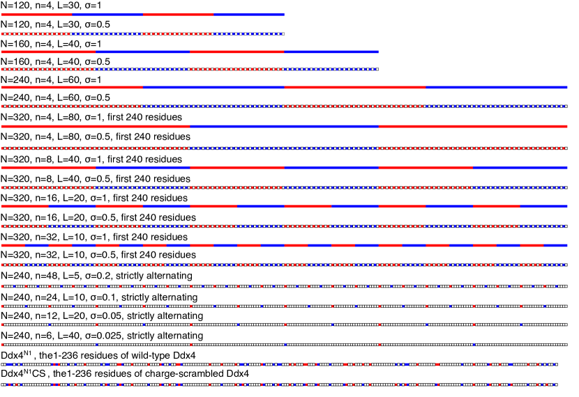
Figure 1: Sequences studied in the present work. Monomers (residues) are depicted as small squares. Each colored square is a monomer with a positive (red) or negative (blue) electronic charge. Neutral monomers are white. For the two Ddx4 sequences, red monomers correspond to either arginine (R) or lysine (K); blue monomers correspond to either aspartic (D) or glutamic (E) acid [30, 92]. $N$ is chain length (number of monomers), $n$, the number of charged blocks, $L$, length of an individual block, and $\sigma$, the fraction of monomers that are charged. The first 14 sequences are studied in Fig. 4, the next four sequences in Fig. 5, and the last two sequences in Figs. 6, 9, and 12. For the $N=320$ sequences, only the first 240 monomers are included in this figure. The other 80 monomers of each of these sequences follow the same charge pattern of the first 240 monomers shown.

We now proceed to add inter-monomer interactions into the system. RPA assumes that the interactions are weak such that the Gaussian-chain geometry described in the bare correlation matrix $\hat{G}$ remains a good approximation for the polyampholytes. In general, sequence dependence of conformational distribution, which is expected physically [52], may be treated approximately by replacing the (bare) Kuhn length $b$ by a sequence-dependent renormalized Kuhn length [89]. For tractability, however, here we assume that $\hat{G}$ is sequence independent. Under this assumption, for any given interaction matrix $\hat{U}_{k}=\hat{u}_{k}/(k_{\rm B}T)$, its perturbative effect on the partition function can be calculated as the average of $\exp(-\hat{U}_{k})$ over all Gaussian-chain configurations,

$$Z_{u}= \frac{\int{\cal D}|\rho_{k}\rangle\exp\left(-\frac{1}{2V}\sum_{k\neq 0}\langle\rho_{-k}|(\hat{G}_{k}^{-1}+\hat{U}_{k})|\rho_{k}\rangle\right)}{\int{\cal D}|\rho_{k}\rangle\exp\left(-\frac{1}{2V}\sum_{k\neq 0}\langle\rho_{-k}|\hat{G}_{k}^{-1}|\rho_{k}\rangle\right)}$$ (28)

$$\times\exp\left(-\frac{1}{2V}\langle\rho_{k=0}|\hat{U}_{k=0}|\rho_{k=0}\rangle\right)$$

$$\equiv Z_{u}^{(1)}Z_{u}^{(2)}\;.$$

Since all eigenvalues of $\hat{G}^{-1}_{k}$ and $\hat{G}^{-1}_{k}+\hat{U}_{k}$ are positive for Coulomb interaction, the path integrals in Eq. (28) can be calculated by Gaussian integrations to yield

$$Z_{u}^{(1)}=\frac{\prod_{k\neq 0}\sqrt{\det\left(\hat{G}_{k}^{-1}\!+\!\hat{U}_{k}\right)}}{\prod_{k\neq 0}\sqrt{\det\left(\hat{G}_{k}^{-1}\right)}}=\prod_{k\neq 0}\sqrt{\det\left(1\!+\!\hat{G}_{k}\hat{U}_{k}\right)}\;.$$ (29)

The $Z_{u}^{(2)}$ factor for $k=0$ depends on the interaction potential $U$. For Coulomb interaction, the neutrality of the system requires [95]

$$\sum_{ij}\rho_{k=0}^{(i)}U_{k=0}^{ij}\rho_{k=0}^{(j)}\propto(\sum_{i}n_{i}q_{i})^{2}=0,$$ (30)

and thus

$$Z_{u}^{(2)}=\exp(0)=1\;.$$ (31)

We hereafter consider $f_{\text{el}}$ for Coulomb interaction as the $f_{\text{int}}$ term in Eq. (1) and calculate it as the logarithm of $Z_{u}^{(1)}$ divided by the total number of lattice sites $V/a^{3}$:

$$f_{\text{el}}=-\frac{a^{3}}{V}\ln Z_{u}^{(1)}=\frac{a^{3}}{2V}\sum_{k\neq 0}\ln[\det(1+\hat{G}_{k}\hat{U}_{k})]\;.$$ (32)

In doing so, we are using $Z_{u}$ in Eq. (28) as the partition function of the system. This is appropriate for phase separation studies because it amounts to choosing as reference state a noninteracting system that does not phase separate and whose partition function is given by the denominator of the first line of Eq. (28). Approximating the summation in Eq. (32) as an integration, $(1/V)\sum_{k}\to\int d^{3}k/(2\pi)^{3}$ [96, 95], and subtracting the self electrostatic energy of all charges to eliminate unphysical “ultraviolet” divergences at $k\!\to\!\infty$ [77, 97, 95, 100], we arrive at the RPA formula [97, 98, 95]

$$f_{\rm el}=\frac{1}{2}\int\frac{d^{3}(ka)^{3}}{(2\pi)^{3}}\left\{\ln[\det(1+\hat{G}_{k}\hat{U}_{k})]-\mathrm{Tr}(\hat{\rho}\;\hat{U}_{k})\right\}.$$ (33)

As in [91], here we consider a Coulomb potential with a short-range physical cutoff on the scale of monomer size [97, 95],

$$U(r)=\frac{l_{B}(1-e^{-r/b})}{r}\;,$$ (34)

where $r$ is spatial distance between electric charges. In $k$-space, this becomes

$$\hat{U}_{k}=\frac{4\pi l_{B}}{k^{2}[1+(kb)^{2}]}|q\rangle\langle q|\equiv\lambda(k)|q\rangle\langle q|\;,$$ (35)

where $l_{B}=e^{2}/(4\pi\epsilon_{0}\epsilon_{r}k_{\rm B}T)$ is the Bjerrum length, $\epsilon_{0}$ is vacuum permittivity, $\epsilon_{r}$ is relative permittivity (dielectric constant) governing the interaction, $|q\rangle$ is the column vector for the charges of the monomers and monovalent ions, and $\langle q|\equiv|q\rangle^{\rm T}$ is the transposed row vector, with components $q_{i}=\sigma_{i}$ for $1\leq i\leq N$, $q_{N+1}=1$, and $q_{N+2}=-1$. The determinant in Eq. (33) can now be simplified as

$$\det(1+\hat{G}_{k}\hat{U}_{k})= 1+\lambda(k)\langle q|\hat{G}_{k}|q\rangle$$ (36)

$$= 1+\lambda(k)\left(2\rho_{s}\!+\!\rho_{c}\!+\frac{\rho_{m}}{N}\!\langle\sigma|\hat{G}_{\mathrm{M}}(k)|\sigma\rangle\right)$$

by using Sylvester’s identity $\det(\hat{I}_{\mu}+\hat{A}\hat{B})=\det(\hat{I}_{\nu}+\hat{B}\hat{A})$ where $\hat{A}$ and $\hat{B}$ are, respectively, any $\mu\times\nu$ and $\nu\times\mu$ matrices and $\hat{I}_{\mu}$ and $\hat{I}_{\nu}$ are, respectively, $\mu\times\mu$ and $\nu\times\nu$ identity matrices [70]. The second term in Eq. (36) is a linear function of $\rho_{m}$, and

$$\ln[\det(1+\hat{G}_{k}\hat{U}_{k})]\xrightarrow{k\to\infty}\lambda(k)\langle q|\hat{G}_{k}|q\rangle.$$ (37)

This limiting property allows us to replace the trace in Eq. (33) by $\lambda(k)\langle q|\hat{G}_{k}|q\rangle$ to facilitate numerical integration for $f_{\text{el}}$ [74]. As will be discussed in Sec. 2.3 and A, the additional term linear in $\rho_{m}$ has no effect on phase separation.

As in [91], a set of dimensionless variables are introduced for our analysis. First, a reduced temperature is defined by rescaling temperature with electrostatic energy,

$$T^{*}\equiv{b}/{l_{B}}={4\pi\epsilon_{0}\epsilon_{r}k_{\rm B}Tb}/{e^{2}}\;.$$ (38)

In addition, the $f_{\text{el}}$ integration is rewritten in terms of the reduced wave number $\tilde{k}=kb$. We notice that $\hat{G}_{\mathrm{M}}(k)$ is a function of $kb$ and thus we rewrite it as $\hat{G}_{\mathrm{M}}(\tilde{k})$. Together with the rescaled densities $\phi_{m}=\rho_{m}a^{3}$, $\phi_{c}=\rho_{c}a^{3}$, and $\phi_{s}=\rho_{s}a^{3}$, $f_{\text{el}}$ may be expressed in terms of dimensionless variables only,

$$f_{\text{el}}=\int\frac{d\tilde{k}\tilde{k}^{2}}{4\pi^{2}}\left\{\frac{1}{\eta}\ln\left[1+\eta{\cal G}(\tilde{k})\right]-{\cal G}(\tilde{k})\right\}\;,$$ (39)

where $\eta=(b/a)^{3}$ is the ratio between the cube of polymer link length and water molecular size when $r_{w}=1$, and

$$\!\!{\cal G}(\tilde{k})=\frac{4\pi}{\tilde{k}^{2}[1+\tilde{k}^{2}]T^{*}}\left(2\phi_{s}\!+\!\phi_{c}\!+\!\frac{\phi_{m}}{N}\langle\sigma|\hat{G}_{\mathrm{M}}(\tilde{k})|\sigma\rangle\right).$$ (40)

Using numerical integration of Eq. (39) for $f_{\rm int}=f_{\text{el}}$ in Eq. (1) and the FH configurational entropy expression in Eq. (13) for $-s$, this formulation is applied below to study the phase behaviors of the sequences in Fig. 1.

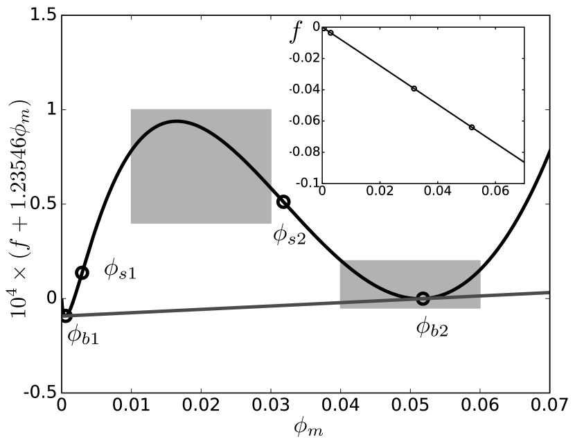
Figure 2: The $f(\phi_{m})$ function [Eq. (1)] at $T^{*}=1/3.5=0.286$ in our RPA model for Ddx4^N1 [91] minus $-1.23546\phi_{m}$, where $-1.23546$ is the slope of the secant from $\phi_{m}=0$ to $0.05$. $f(\phi_{m})$ itself is shown in the inset. $\phi_{s1}$, $\phi_{s2}$ are the two spinodal points satisfying $f^{\prime\prime}_{el}(\phi_{m})=0$, whereas $\phi_{b1}$, $\phi_{b2}$ are the two binodal points sharing a common tangent. The $f$ values for these four $\phi_{m}$’s are marked by circles. The subtraction of a term linear in $\phi_{m}$ from $f(\phi_{m})$ serves to better exhibit its curvature, which is less apparent visually without the subtraction (inset). The two shaded boxes mark two regions of $f(\phi_{m})$ that are further analyzed, respectively, in Fig.3b and 3c.

2.3 Determination of phase boundaries

We first use the RPA model for Ddx4^N1 with $r_{m}=r_{c}=r_{s}=r_{w}=1$ [91] as an example to illustrate the procedure used to determine phase boundaries (Figs. 2 and 3) and to highlight qualitative differences between RPA and FH phase behaviors (cf. Fig. 4 of [27]). The charge pattern of Ddx4^N1 is provided in Fig. 1.

Figure 3: Phase stability of the RPA model for Ddx4 [91]. Shown here are enlarged parts of the $f(\phi_{m})$ function in Fig. 2. (a) Zoom-in display of the low-$\phi_{m}$ minimum of $f(\phi_{m})$ near the origin. (b) The convex region of $f(\phi_{m})$ satisfying Eq. (44). (c) The concave region near the second minimum of $f(\phi_{m})$. This region satisfies the inequality reverse to that of Eq. (44).

Using the configurational entropy and interaction terms in Eqs. (13) and (39), the free energy of Ddx4^N1 solution is a function of polyampholyte and salt densities,

$$f=f(\phi_{m},\phi_{s})\;.$$ (41)

Whether concentrations $(\phi_{m},\phi_{s})$ result in phase separation depends on the local curvature of $f$ on the $\phi_{m}-\phi_{s}$ plane. We consider only the salt-free ($\phi_{s}=0$) case in Figs. 2 and 3. The function $f$ exhibits two local minima (Fig.  2), one at $\phi_{m}\approx 0.005$ (Fig. 3a), the other at $\phi_{m}\approx 0.052$ (Fig. 3c). Two points in Fig. 2, $\phi_{m}=\phi_{s1}$, $\phi_{s2}$, satisfy

$$f^{\prime\prime}\equiv\frac{d^{2}f}{d\phi_{m}^{2}}=0\;.$$ (42)

The free energy is a concave function ($f^{\prime\prime}<0$) between these two points. Consider two concentrations $\phi_{m}^{(1)}<\phi_{m}^{(2)}$ within this region. Any $\phi_{m}$ in between these two concentrations, i.e., $\phi_{m}^{(1)}\leq\phi_{m}\leq\phi_{m}^{(2)}$, can be written as

$$\phi_{m}=v_{1}\phi_{m}^{(1)}+v_{2}\phi_{m}^{(2)}\;,$$ (43)

where the weight factors $v_{1}$,$v_{2}$ satisfy $0\leq v_{1},v_{2}\leq 1$. A homogeneous concentration $\phi_{m}$ is not stable in the concave region because its free energy is higher than the free energy $\bar{f}$ of two phase-separated (demixed) concentrations $\phi_{m}^{(1)}$ and $\phi_{m}^{(2)}$,

$$\bar{f}=v_{1}f(\phi_{m}^{(1)})+v_{2}f(\phi_{m}^{(2)})<f(v_{1}\phi_{m}^{(1)}+v_{2}\phi_{m}^{(2)})\;,$$ (44)

as can be seen in Fig. 3b by comparing the free energy values along the secant from $\phi_{m}^{(1)}$ to $\phi_{m}^{(2)}$ and $f$ itself. In contrast, in a region with $f^{\prime\prime}>0$, the homogeneous phase is seen to be more favorable by using the same consideration (Fig. 3c). The $f^{\prime\prime}<0$ condition defines the spinodal phase separation region in which the demixed state is globally more favorable. For systems with more than two relevant molecular components, i.e. $f=f(\{\phi_{k}\})$, the spinodal condition Eq. (42) is generalized to

$$\det{\hat{\cal F}}=0\;,\;\hat{\cal F}_{ij}=\frac{\partial^{2}f(\{\phi_{k}\})}{\partial\phi_{i}\partial\phi_{j}}\;.$$ (45)

As is conventional, the phase boundaries in [91] are coexistence curves satisfying the binodal condition, which corresponds to the equality of chemical potentials across phase boundaries, and therefore may be determined graphically by constructing a common tangent (Fig. 2) – because chemical potentials are by definition derivatives of free energy with respect to number of molecules. Specifically, the binodal concentrations $(\phi_{m}^{\alpha},\phi_{m}^{\beta})$ for two separate phases $\alpha,\beta$ is determined by the conditions

$$f^{\prime}(\phi_{m}^{\alpha})= f^{\prime}(\phi_{m}^{\beta})\;,$$ (46a)

$$f(\phi_{m}^{\alpha})-\phi_{m}^{\alpha}f^{\prime}(\phi_{m}^{\alpha})= f(\phi_{m}^{\beta})-\phi_{m}^{\beta}f^{\prime}(\phi_{m}^{\beta}),$$ (46b)

where $f^{\prime}(\phi_{m})=\partial f/\partial\phi_{m}$. These two equations uniquely define the common tangent of $f(\phi_{m})$ at $\phi_{m}^{\alpha}$ and $\phi_{m}^{\beta}$ [101, 27, 102], as illustrated by the example in Fig. 2 with $\phi_{m}^{\alpha}$ and $\phi_{m}^{\beta}$ corresponding to $\phi_{b1}$ and $\phi_{b2}$. While the spinodal region necessitates global phase separation across the entire solution, phase separation can occur locally in binodal regions (e.g., for bulk concentration $\phi_{m}$ in the regions $\phi_{b1}<\phi_{m}<\phi_{s1}$ and $\phi_{s2}<\phi_{m}<\phi_{b2}$ in Fig. 2). In these regions, strong local fluctuations into the spinodal region can be metastable, resulting in small liquid droplets with a different concentration. Generalizations of the bionodal conditions in Eq. (46) are provided in A.

It should be noted that salt concentration $\phi_{s}$ is taken to be uniform (constant across phase boundaries) here and in [91]. This need not be the case in general. Indeed, two-phase electrostatic coacervation in systems consisting of two, three, and four types of charged molecules have been well studied under the framework of DH theory [103, 101, 104, 105]. Previous research, however, suggests that change in salt concentration is insignificant upon biological coacervation [104, 81]. We therefore assume for simplicity that the phase behavior of our model polyampholyte system does not involve fluctuation in salt concentration.

3 Phase behaviors of salt-free block polyampholytes

To better understand the physical consequences of our RPA model and to delineate its differences with FH theory in detail, we extend our previous analysis [91] of simple salt-free ($\rho_{s}=0$) solutions of polyampholytes consisting of $n$ alternating charge blocks (labeled by $\alpha$, $\beta=1$, 2, $\dots,n$) with length $L\!=\!N/n$. The charge density in each block is $\sigma_{\alpha}^{\text{block}}=(-1)^{\alpha-1}\sigma$, i.e., a charge per $1/\sigma$ monomers (Fig. 1). For simplicity, we assume, as before [91], that all monomers are of identical size, i.e. $r_{m}=r_{c}=r_{s}=1$, and the polymer link length is equal to the solvent length scale, i.e., $b=a$ [$\eta=1$, Eq. (39)].

The correlation matrix $\hat{G}_{\mathrm{M}}(\tilde{k})$ for these highly regular charge patterns is reduced to an $n\times n$ matrix for the blocks, $\hat{G}_{\mathrm{M}}^{\text{block}}(k)$. The diagonal terms of $\hat{G}_{\mathrm{M}}^{\text{block}}$,

$$\hat{G}_{\mathrm{M}}^{\text{block}}(k)_{\alpha\alpha}=\sum_{i,j=1}^{L}\sigma_{i}\sigma_{j}e^{-(kb)^{2}|i-j|/6}\;,$$ (47)

account for intra-block correlations. Because only the $(1+l/\sigma)$th ($l=0,1,2,...$) residues are charged, as illustrated by the second sequence in Fig. 1, the summation of $\hat{G}_{\mathrm{M}}^{\text{block}}$ becomes

$$\hat{G}_{\mathrm{M}}^{\text{block}}(k)_{\alpha\alpha}=\sum_{i,j=1}^{L\sigma}e^{-(kb)^{2}|i-j|/(6\sigma)},$$ (48)

in which the $i$ and $j$ labels only go through the charged residues. The $\hat{G}_{\mathrm{M}}^{\text{block}}(k)_{\alpha\alpha}$ is then calculated in terms of $\zeta\equiv$ $\exp(-(kb)^{2}/(6\sigma))$ as

$$\hat{G}_{\mathrm{M}}^{\text{block}}(k)_{\alpha\alpha}= L\sigma+2\sum_{j=1}^{L\sigma}\sum_{i=j+1}^{L\sigma}\zeta^{i-j}$$ (49)

$$= \frac{1+\zeta}{1-\zeta}L\sigma-\frac{2\zeta(1-\zeta^{L\sigma})}{(1-\zeta)^{2}}\;,$$

where the $L\sigma$ term corresponds to the self-correlation of each charged monomer. The off-diagonal terms account for inter-block correlations, of which the lower triangular components ($\alpha>\beta$) are

$$\hat{G}_{\mathrm{M}}^{\text{block}}(\tilde{k})_{\alpha>\beta}=\sum_{i=(\alpha-1)L\sigma+1}^{\alpha L\sigma}\sum_{j=(\beta-1)L\sigma+1}^{\beta L\sigma}\zeta^{i-j}$$ (50)

$$= \frac{\zeta^{(\alpha-1)L\sigma+1}(1-\zeta^{L\sigma})}{1-\zeta}\times\frac{\zeta^{-(\beta-1)L\sigma-1}(1-\zeta^{-L\sigma})}{1-\zeta^{-1}}$$

$$= \frac{\zeta}{(1-\zeta)^{2}}\zeta^{(\alpha-\beta-1)L\sigma}(1-\zeta^{L\sigma})^{2}$$

and the upper triangular part is given by switching $\alpha$ and $\beta$, resulting in the general expression

$$\hat{G}_{\mathrm{M}}^{\text{block}}(k)_{\alpha\beta}=\frac{\zeta}{(1-\zeta)^{2}}\zeta^{(|\alpha-\beta|-1)L\sigma}(1-\zeta^{L\sigma})^{2}\;.$$ (51)

In the same vein, $|\sigma\rangle$ is grouped into $n$ components with $\sigma_{\alpha}=(-1)^{\alpha-1}$. The RPA contribution from $\hat{G}_{\mathrm{M}}$ is then calculated by summing all $\hat{G}_{\mathrm{M}}^{\text{block}}(k)$ elements with alternating $\pm 1$ weight factors, yielding

$$\langle\sigma|\hat{G}_{\mathrm{M}}(k)|\sigma\rangle$$ (52)

$$=n\hat{G}_{\mathrm{M}}^{\text{block}}(k)_{\alpha\alpha}+2\sum_{\beta=1}^{n}\sum_{\alpha=\beta+1}^{n}(-1)^{\alpha-\beta}\hat{G}_{\mathrm{M}}^{\text{block}}(k)_{\alpha\beta}$$

$$=\frac{1+\zeta}{1-\zeta}nL\sigma-\frac{2\zeta}{(1-\zeta)^{2}}(1-\zeta^{L\sigma})n$$

$$\quad+\frac{2\zeta^{1-L\sigma}}{(1-\zeta)^{2}}(1-\zeta^{L\sigma})^{2}\sum_{\beta=1}^{n}\sum_{\alpha\!=\!\beta+1}^{n}(-\zeta^{L\sigma})^{\alpha-\beta}$$

$$=N\left[\sigma\frac{1+\zeta}{1-\zeta}-\frac{1}{L}\frac{4\zeta}{(1-\zeta)^{2}}\left(\frac{1-\zeta^{L\sigma}}{1+\zeta^{L\sigma}}\right)\right]$$

$$\quad+\frac{2\zeta}{(1-\zeta)^{2}}\left(\frac{1-\zeta^{L\sigma}}{1+\zeta^{L\sigma}}\right)^{2}(1-(-1)^{n}\zeta^{N\sigma})\;.$$

Here we begin by using these formulas to examine phase separation of neutral block polyampholytes ($n$ even and thus $\rho_{c}=0$). The general trend shown in Fig. 4 is that polyampholytes with greater $N$, fewer $n$, and greater $\sigma$ phase separate at higher temperature $T^{*}$. Specifically, when the number of charge blocks, $n$, is fixed, the critical temperature $T^{*}_{\mathrm{cr}}$ (maximum $T^{*}$ of the phase boundary) increases whereas the critical volume fraction (concentration) $\phi_{\mathrm{cr}}$ ($=\phi_{m}$ at $T^{*}_{\mathrm{cr}}$) decreases as the block length $L$ increases (Fig. 4a). This $T^{*}_{\mathrm{cr}}\to\infty$, $\phi_{\mathrm{cr}}\to 0$ trend as $N=nL\to\infty$ with fixed $n$ is consistent with previous reports for short diblock polyampholytes [79, 80]. In the limit of $N\to\infty$, the first term in Eq. (52), which diverges at $k\to 0$, dominates the integration for $f_{\rm el}$. As a result, $f_{\rm el}$ is in the form of the Eq. (5) in Ref. [77] with $\lambda=1$, proportional to $\phi_{m}^{3/2}$ as in Debye-Hückel theory but with an infinitely large prefactor. In this limit, the block number $n$ becomes irrelevant and the system behaves just like a solution of diblock polyampholytes with $N\to\infty$, in which electrostatic interaction is so strong that the RPA is broken. Diblock polyampholytes are expected to form structural aggregates [77, 72]. We note that this $f_{\rm el}$ is much stronger than the Debye-Hückel theory for electrostatic coacervation that expects an $f_{\rm el}$ with a finite prefactor [81].

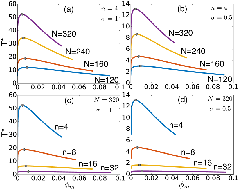
Figure 4: Binodal phase boundaries for neutral salt-free polyampholytes with diffirent combinations of $N$, $n$, and $\sigma$: (a, b) $N=120$, 160, 240, and 320; $n=4$. (c, d) $N=320$, $n=4$, 8, 16, and 32. (a, c) $\sigma=1$. (b, d) $\sigma=0.5$. The dots mark the critical points. Longer polyampholytes (larger $N$) with fewer blocks (smaller $n$) and higher charge densities (higher $\sigma$) have stronger tendencies to phase separate.

If the chain length $N$ is fixed, when $L$ decreases (i.e. $n$ increases), the first term in Eq. (52) is unchanged, but the second term increases, and the third term slightly decreases. In the limit of $N\gg 1$, only the first two $O(N)$ terms are relevant, which yield a decreasing contribution to $f_{\text{el}}$ when $L$ decreases. As shown in Fig. 4, a smaller $T^{*}_{\mathrm{cr}}$ thus results from more but shorter charge blocks, qualitatively consistent with experiment on the charge-scramble mutant Ddx4^N1CS [30]. The increase of $n$ will ultimately arrive at the strictly alternating polyampholyte, in which the polyampholyte contribution to $f_{\rm el}$ integration is given by substituting $L=1/\sigma$ in Eq. (52) to give

$$\frac{1}{N}\langle\sigma|\hat{G}_{\mathrm{M}}(k)|\sigma\rangle=\frac{1-\zeta}{1+\zeta}\sigma+\frac{1}{N}\frac{2\zeta(1-(-1)^{n}\zeta^{N\sigma})}{(1+\zeta)^{2}}\;.$$ (53)

In the limit of $N\to\infty$, only the first term in Eq. (53) remains. As this term converges to $0$ when $k\to 0$, the $f_{\rm el}$ behavior in low $\phi_{m}$ can be evaluated by expanding Eq. (39) using $\ln(1+x)\approx 1+x-x^{2}/2!+...$ to the second order of $\phi_{m}$, yielding

$$f_{\text{el}}^{\infty}\approx -\frac{(6\sigma)^{\frac{3}{2}}}{2}\int\frac{dk^{\prime}k^{\prime 2}}{4\pi^{2}}\left(\frac{4\pi\phi_{m}}{6k^{\prime 2}(1+6\sigma k^{\prime 2})T^{*}}\frac{1-e^{-k^{\prime 2}}}{1+e^{-k^{\prime 2}}}\right)^{2}$$ (54)

$$\equiv -\chi_{\rm el}^{\infty}\phi_{m}^{2}$$

with $k^{\prime 2}=(kb)^{2}/6\sigma$. The electrostatic energy now becomes a quadratic term of polymer concentration. Thus, the $N\to\infty$ alternating polymers are interacting in terms of an effective FH interaction with the FH $\chi$ parameter

$$\chi_{\rm el}^{\infty}=\frac{(6\sigma)^{\frac{3}{2}}}{18T^{*2}}\int\frac{dk^{\prime}}{k^{\prime 2}(1+6\sigma k^{\prime 2})^{2}}\left(\frac{1-e^{-k^{\prime 2}}}{1+e^{-k^{\prime 2}}}\right)^{2}\;.$$ (55)

For weakly charged polyampholytes, $\sigma\ll 1$. Thus, the $(1+6\sigma^{\prime}k^{\prime 2})$ factor in Eq. (55) can be approximated to $1$ as if the short range cutoff is irrelevant, resulting in

$$\chi_{\rm el}^{\infty}\approx 0.687\sigma^{3/2}T^{*-2},$$ (56)

which is equivalent to Eq. (3) in Ref. [77].

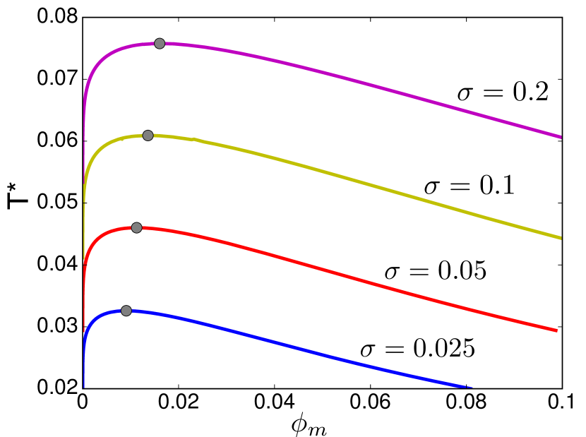
Figure 5: Phase diagrams for strictly alternating polyampholytes with $N=240$ and $\sigma=0.025$, 0.05, 0.1, and 0.2, corresponding to $n=6$, 12, 24, and 48, respectively. Critical points are marked by the gray circles. Smaller $\sigma$ leads to lower $\phi_{\mathrm{cr}}$ and lower $T^{*}$.

The critical point, however, does not obey the FH result that $\phi_{\mathrm{cr}}\approx 1/\sqrt{N}$ and $\chi_{\rm el}^{\infty}=0.5$. First, the second $O(1/N)$ term in Eq. (53) enhances $f_{\text{el}}$, and thus $\phi_{\mathrm{cr}}$ is smaller than the FH result. Even without considering this $1/N$ term in $f_{\text{el}}$, an approximate description of these RPA results by a FH framework is still not applicable because FH does not take into account higher order terms of $\phi_{m}$. In the calculation of critical point, both the second and third order derivatives of free energy have to be zero. As FH only includes interactions up to $O(\phi_{m}^{2})$, the third order derivative of interaction energy must be zero. The exact $f_{\text{el}}$ in RPA, however, can be expanded further,

$$f_{\text{el}}^{\infty}(\phi_{m})=f_{\text{el}}^{\infty}(\phi_{m}\!=\!0)-\frac{1}{2}A\phi_{m}^{2}+\frac{1}{6}B\phi_{m}^{3}+O(\phi_{m}^{4}),$$ (57)

where $A=2\chi_{\rm el}^{\infty}$ and $B=\partial^{3}f_{\text{el}}(\phi_{m}\!=\!0)/\partial\phi_{m}^{3}$ is given by

$$B=2(6\sigma)^{\frac{3}{2}}\int\frac{dk^{\prime}k^{\prime 2}}{4\pi^{2}}\left(\frac{4\pi}{6k^{\prime 2}(1+6\sigma k^{\prime 2})T^{*}}\frac{1-e^{-k^{\prime 2}}}{1+e^{-k^{\prime 2}}}\right)^{3},$$ (58)

which in the limit of $\sigma\ll 1$ becomes

$$B\approx 1.187\sigma^{3/2}T^{*-3}.$$ (59)

Noted that $\chi_{\rm el}^{\infty}=0.5$ in Eq. (56) would result in $T^{*}\sim\sigma^{3/4}$ and thus $B\sim\sigma^{-3/4}\gtrsim 1$, contradicting with the requirement of $B\approx 0$ in FH theory.

Because the third order derivative of $f_{\text{el}}$ as well as the finite-size effect from $N$ and $\sigma$ are not negligible in our RPA model, the FH inference based on Eq. (56) does not lead to the correct critical point. In B we describe a semi-analytic solution for critical point in the limit of $N\to\infty$ for any $\sigma$. Phase diagrams of a series of strictly alternating polyampholytes with identical $N$ are shown in Fig. 5. In contrast to the decreasing $T^{*}_{\mathrm{cr}}$ and increasing $\phi_{\mathrm{cr}}$ with increasing number of charge blocks $n$ when charge density $\sigma$ is fixed (Fig. 4c,d), when the charge per block is fixed as in Fig. 5, both $T^{*}_{\mathrm{cr}}$ and $\phi_{\mathrm{cr}}$ increase with increasing number of charge blocks $n$. In other words, whereas the variations of $T^{*}_{\mathrm{cr}}$ and $\phi_{\mathrm{cr}}$ in Fig. 4 impact phase separation in the same direction, the variations of $T^{*}_{\mathrm{cr}}$ and $\phi_{\mathrm{cr}}$ for strictly alternating polyampholytes in Fig. 5 are such that they have opposite effects on the tendency of the solution to phase separate.

4 Comparison of RPA and other analytical models for Ddx4 phase separation

4.1 The RPA model

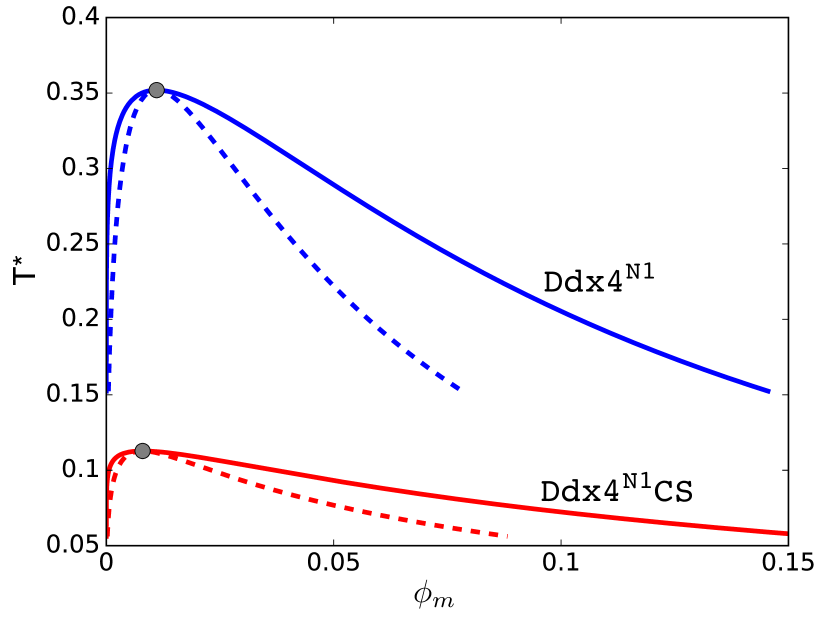
Figure 6: The salt-free phase diagrams for the two Ddx4 sequences in our RPA theory. Solid lines are binodal boundaries that have been shown in [91], dashed lines are spinodal boundaries. Gray circles mark the critical points. In this theory, $T^{*}_{\mathrm{cr}}$ of Ddx4${}^{\text{N1}}$CS is $\approx 1/3$ that of Ddx4${}^{\text{N1}}$.

We have applied our RPA theory to Ddx4 by considering the exact amino acid sequences of residues 1–236 of wildtype Ddx4 (Ddx4${}^{\text{N1}}$) and its charge-scrambled mutant (Ddx4${}^{\text{N1}}$CS) [30] (Fig. 1) to compute their binodal [91] and spinodal boundaries (Fig. 6). In this calculation, we assume for simplicity $r_{m}=r_{c}=r_{s}=\eta=1$. We have considered the general size-dependent formulation in Sec. 2.1 with reasonable variations in monomer sizes and found that the variations we tested only resulted in shifts of the phase boundaries in the vertical ($T^{*}$) direction without much alternation of their overall shapes. Consistent with the experimental observation that Ddx4${}^{\text{N1}}$ phase separates but Ddx4${}^{\text{N1}}$CS does not [30], Fig. 6 indicates that Ddx4${}^{\text{N1}}$CS with its scrambled charged pattern has a critical temperature $T^{*}_{\rm cr}$ that is only about 1/3 that of the wildtype in our RPA model [91]. However, the critical concentration $\phi_{\mathrm{cr}}$ of Ddx4${}^{\text{N1}}$CS is larger, not smaller, than that of the wildtype. This trend of $(T^{*}_{\rm cr},\phi_{\mathrm{cr}})$ variation is reminiscent of the $\sigma$ dependence of strictly alternating polyampholytes in Fig. 5.

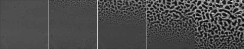
Figure 7: Spinodal behavior of Ddx4. The montage shown was obtained by drying a droplet of Ddx4 in aqueous buffer solution and recorded using a 10x objective. The time lapse between successive frames (from left to right) was 0.32 second. The edge of the circular drying droplet was on the top of the frame though well out of view. Consequently, evaporation and hence increase in Ddx4 concentration was proceeding from top to bottom, resulting in the upper parts reaching the spinodal regime before the lower parts of the frame (courtesy Timothy J. Nott, unpublished).

The coexistence of two phases in Ddx4^N1 solution has been characterized experimentally by a dramatic change of turbidity by lowering temperature – presumably as the system crosses the binodal boundary – when numerous droptlets with relatively higher concentration of Ddx4 are formed (Fig. 3D in Ref. [30]). Global spinodal phase separation of Ddx4^N1 solution has also been observed by rapid increase in concentration, probably quenching the system well into the spinodal regime. In this case, no spherical droplets were formed. Instead, the condensed regions extended and then merged into a giant network (Fig. 7).

4.2 Proposed analytical models for IDP phase separation

We now proceed to compare models that have been either applied to [30, 91] or proposed for [33] the study of IDP phase separation. These include the FH [30] and RPA [91] models for Ddx4, and the OV/DH approach advocated in a recent review on the polymer physics of intracellular phase transitions [33]. All these models are mean-field at one level in that they all incorporate the classical FH lattice derivation of configurational entropy described here in Sec. 2.1, which considers only bulk polymer concentration and ignores all local density fluctuation. However, the way interactions within and among polymers are treated is quite different in these models.

In both FH and OV/DH, the amino acid residues in polypeptides are treated as independent monomers. Chain connectivity is only accounted for in a mean-field manner in the derivation of configuration entropy (the $(z-1)$ factors in Eq. (6); but this factor is irrelevant to phase separation). But chain connectivity is neglected entirely in the interaction term, precluding these theories from addressing sequence-dependent interactions directly. For example, the FH model for Ddx4 in [30] uses a single overall FH $\chi$ parameter as an average interaction strength. It does not distinguish between charged and uncharged residues. Moreover, the derivation of FH assumes that interactions are of short-range, point-contact type [58, 69]. As such, the applicability of FH to long-range Coulomb interactions may be limited, as is evident from the difference in $\phi_{m}$ dependence between its interaction term and that of OV/DH (see below). The OV/DH approach recognizes charged and neutral residues so as to apply electrostatic interaction only to the former, but it does not distinguish between positive and negative charges. Only the total number of charged monomers, counterions, and salt ions can be parametrized [60]. Thus, in contrast to the RPA approach that offers a direct treatment of charge pattern along the polypeptide sequence [91], effects of charge pattern are absent in FH and OV/DH models. The consequences of the assumptions in these models are examined below by applying them to the salt-dependent phase behavior of Ddx4^N1.

To compare the model results with experiment, we equate $a^{3}$ with the volume of a single water molecule in all calculation below. Accordingly, the volume fraction of amino acid residues is given by $\phi_{m}$ $=236$[Ddx4]/(55.5 M) because [H₂O] = 55.5 M. We restrict our consideration to salt concentrations $\phi_{s}=$ 0.0018, 0.0027, 0.0036, and 0.0054, which correspond, respectively, to [NaCl]=100, 150, 200, and 300 mM [91] that have been investigated experimentally [30]. To faciliate comparison with the experimental phase diagrams in Fig. 4 of [30], special focus is placed on the range of [Ddx4]=0 – 400$\mu$M.

4.3 Flory-Huggins (FH) model

FH model has been applied to analyze experimental data of Ddx4 phase separation [30]. This particular model supposes that Coulomb interaction contributes to attraction between all residue pairs, and the effect of salt is a screening effect that decreases this general attraction. Following the description of the model in Supplemental Information of [30], we conducted the calculation anew, arriving at a set of parameters that provide a reasonably good fit to the experimental data (Fig. 8a, inset). Our fitted parameters were obtained by first fixing $\Delta H_{0}$ and $\epsilon_{r}$ to values consistent with those in [30]. The resulting parameters differ from theirs, however, probably because there can be more than one optimum for such a multiple-parameter fit. Nonetheless, in agreement with [30], we found within the [NaCl] range studied that the entropic contribution $\Delta S$ to the FH $\chi$ parameter is always negative, meaning that entropy favors phase separation.

The full FH phase diagrams are provided in Fig. 8a. Three features are notable. First, the FH phase boundaries always concave downward, whereas RPA phase boundaries are S-shaped with inflection points, i.e., part of it convex downward (Fig. 6). Second, FH predicts a salt-independent critical concentration, $\phi_{\mathrm{cr}}\approx 1/\sqrt{N}$. Third, the FH phase boundaries of different salt concentrations cross at $T\approx 100^{\circ}$C, exhibiting opposite tendency above and below this temperature. These features, which are testable by experiment in principle, are not presented in the corresponding RPA phase boundaries, as will be discussed in Sec. 4.5 below.

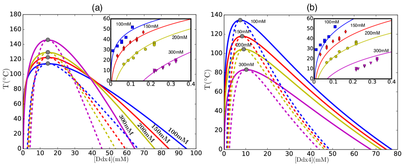
Figure 8: Salt-dependent phase diagrams of Ddx4${}^{\text{N1}}$ predicted by different theories and their comparison with experimental [NaCl] dependence. Binodal and spinodal boundaries are shown, respectively, as solid and dashed lines. Critical points are marked by gray circles. Experimental data [30] are included in the insets for comparison (symbols; same color code). (a) FH theory in Ref. [30] as described in the Supplemental Information of this reference. The fitting parameters are $\Delta H_{0}=78$ J mol^-1, $\epsilon_{r}=50$, $r_{d}=8.4354$Å, $\Delta S_{0}=-10.4922$ J mol^-1K^-1, and $B_{0}=-0.19549$ (the last two parameters are for Eq. [S20] of [30] in the form of $\Delta S=\Delta S_{0}+B_{0}R\ln([{\rm NaCl}]/55.5)$, where [NaCl] is in M). The critical point is always at $\phi_{\mathrm{cr}}\approx 1/\sqrt{N}$ and $\chi_{\rm cr}\approx 0.5+1/\sqrt{N}$ because these values are fixed in the FH model [69]. (b) DH theory given by $f_{\rm DH}$ in Eq. (60); $\epsilon_{r}=59.5$ is used to convert $T^{*}$ to $T$(^∘C) to fit the experimental data.

4.4 The Overbeek-Voorn/Debye-Hückel (OV/DH) model

The OV/DH model is based on the linearized Poisson-Boltzmann equation, which self-consistently calculates the screening effect of monomeric ions [81, 61]. To apply DH to polyampholytes such as Ddx4, we count all charged residues as independent monomeric ions and calculate the electrostatic energy as

$$f_{\rm DH}=-\frac{1}{12\pi}\left(\frac{4\pi[(\phi_{m}/N)(\sum_{i}|\sigma_{i}|+|\sum_{i}\sigma_{i}|)+2\phi_{s}]}{T^{*}}\right)^{3/2}\;.$$ (60)

In salt-free solution, the OV/DH model entails an interaction $\propto\phi_{m}^{3/2}$, instead of $\propto\phi_{m}^{2}$ in FH. as noted recently in the context of IDP phase separation [33]. Because $\partial^{2}\phi_{m}^{3/2}/\partial\phi_{m}^{2}$ $\sim$ $\phi_{m}^{-1/2}$, it predicts a $\phi_{m}$ dependence that is much sharper than the corresponding constant term in FH. This feature reflects the long-range nature of electrostatic interactions and allows phase separation to occur under much more dilute concentrations.

To compare OV/DH model predictions with experiment, values for the link length scale $b$ and dielectric constant $\epsilon_{r}$ are needed in Eq. (38) to convert the reduced temperature $T^{*}$ in the model to actual temperature. As in our previous RPA work, we take $b$ to be the C$\alpha$-C$\alpha$ virtual bond length 3.8Å, and let $\epsilon_{r}$ be a fitting parameter [91], as $\epsilon_{r}$ of an aqueous protein solution can vary widely between $\approx$ 2 and 80 [106, 107, 108]. A dielectric constant $\epsilon_{r}=59.5$ resulted from fitting with experimental data (Fig. 8b, inset). The corresponding DH phase diagrams are provided in Fig. 8b. In comparison with the FH phase diagrams in Figs. 8a, OV/DH predicts lower $T^{*}_{\mathrm{cr}}$ and salt-dependent $\phi_{\mathrm{cr}}$ instead of the salt-independent $\phi_{\mathrm{cr}}$ in FH. Unlike FH, the phase boundaries of OV/DH model do not cross each other.

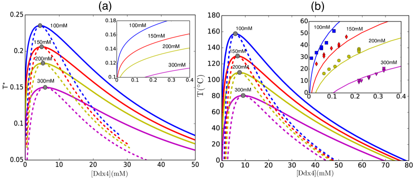
Figure 9: (a) Theoretical phase diagrams of Ddx4${}^{\text{N1}}$ with different [NaCl]’s, computed by (a) Eq. (33), the RPA-only theory, and (b) Eq. (33) with Eq. (61), the RPA+FH theory. Binodal and spinodal boundaries are shown, respectively, as solid and dashed lines. Critical points are marked by gray circles. The two insets highlight the phase behavior for small Ddx4 concentration for which experimental data are availabe [30] (shown as symbols with the same color code in the inset of (b)). Data in the insets were provided previously [91] and are included here for completeness.

4.5 An augmented RPA model

We recently applied RPA and an augmented RPA+FH model to the salt-dependent phase behavior of Ddx4^N1 [91], focusing only on the low [Ddx4] regime for which experimental data are available (Fig. 9, insets). Here we extend that theoretical study to explore essentially the entire binodal and spindoal boundaries of Ddx4^N1 at four [NaCl]’s (Fig. 9), and compare their properties with the FH and OV/DH theories discussed above.

Our RPA model for Coulomb interaction may be viewed as a one-step improvement from the DH model. As described in Sec. 2, RPA treats polymers as Gaussian chains without excluded volume. It allows a direct plug-in of any given charge pattern onto the chain sequence. Different charge patterns distribute their interactions over the Gaussian-chain conformations differently. Therefore, despite the approximations involved in RPA [70, 72], it does provide an account of sequence dependence that is absent in the FH and OV/DH approaches. In particular, RPA allows us to rationalize and gain insights into the different behaviors of Ddx4^N1 and Ddx4^N1CS (Fig. 6) [91], which is not possible, at least not in any conceptually clear manner, for FH and OV/DH. In the special case when the polymer length in RPA is equal to one, RPA is reduced to DH.

Similar to the OV/DH phase boundaries in Fig. 8b, the RPA phase boundaries of different [NaCl]’s calculated using Eq. (33) do not cross each other (Fig. 9a). Notably, the RPA phase boundaries are S-shaped, unlike the inverted U-shaped curves in FH (Fig.8a). For the OV/DH model, the spinodal boundaries are also clearly S-shaped; some of the binodal boundaries are also slightly S-shaped (Fig.8b), but not as pronounced as for the RPA and RPA+FH models. S-shaped phase boundaries in RPA models have also been reported in polyelectrolyte systems, and have been proposed in those cases as a consequence of formation of a polymer network in the solution [74]. In the context of IDP phase separation, S-shaped phase boundaries may help rationalize the possibility of having a relatively low IDP concentration even in the phase-separated IDP-rich phase. So far our RPA+FH theory has only been tested within a very narrow low concentration range for which experimental data are available (inset of Fig. 9b). More extensive experimental data and numerical simulations will be needed to test the theoretically predicted phase boundary to the right of the critical point.

As we have pointed out in [91], while RPA rationalizes the trend of salt dependence (Fig. 9a, inset), RPA by itself does not account for the effect quantitatively. For this reason and the physical consideration that short-range aromatic cation-$\pi$ and $\pi$-$\pi$ interactions [109, 110] are important for IDP interactions in general [12, 111, 30, 112, 33, 113] and play a significant role in Ddx4 phase separation in particular [30], we constructed an RPA+FH model by augmenting the $f_{el}$ in Eq. (33) with the following salt-independent FH interaction term,

$$f_{\rm FH}=\chi\phi_{m}(1-\phi_{m})=\left(\frac{\varepsilon_{h}}{T^{*}}+\varepsilon_{s}\right)\phi_{m}(1-\phi_{m})\;,$$ (61)

such that the $f_{\rm int}$ in the total free energy $f$ in Eq. (1) becomes

$$f_{\rm int}=f_{\rm el}+f_{\rm FH}\;.$$ (62)

Here $\varepsilon_{h}$ and $\varepsilon_{s}$ are the enthalpic and entropic contributions, respectively, to the FH interaction parameter $\chi$. By treating $\varepsilon_{h}$ and $\varepsilon_{s}$ as global fitting parameters, a reasonably good fit is achieved with experimental results for all four available [NaCl] values [30] (Fig. 9b, inset) by using a value of $\epsilon_{r}=29.5$ which is physically plausible for a low-concentration IDP solution (see Sec. 5 below). The overall shapes of the phase boundaries remain largely unchanged vis-à-vis those predicted by RPA (cf. Fig. 9a and b). Similar to the OV/DH model (Fig. 8b), the critical concentration increases with increasing salt in both the RPA and RPA+FH models, in contrast to the salt-independet critical concentration predicted by FH (Fig. 8a).

As we have discussed previously, the fitted $\varepsilon_{h}=0.15$ and $\varepsilon_{s}=-0.3$ used to produce Fig. 9b may be rationalized to an extent by considering the strength of cation-$\pi$ interactions as well as the expected loss of sidechain conformational entropy upon formation of such contacts [91]. Of course, given that RPA is an approximate approach, $f_{\rm FH}$ may also serve to correct inaccuracies in the pure-RPA theory. Finally, it is noteworthy that our fitted entropic free energy $\varepsilon_{s}=-0.3$ is negative, which means that the entropy in the FH $\chi$ parameter is positive (because of the $-T$ factor needed to convert entropy to free energy). Hence the entropy in our FH $\chi$ disfavors phase separation whereas that in the FH model in Sec. 4.3 favors phase separation. Nonetheless, the two results are not necessarily inconsistent because there are additional contributions to conformational entropy in the RPA $f_{\text{el}}$, namely the $\hat{G}_{k}$ in Eq. (33) that accounts for conformational freedom of Gaussian chains.

5 Possible cooperativity-enhancing effects of concentration dependent relative permittivity

In all the theories considered above, the relative permittivity, or dielectric constant $\epsilon_{r}$, is considered to be a constant throughout the solution irrespective of whether the system has phase separated. However, because proteins have very different relative permittivity ($\epsilon_{r}\approx 2$ – $4$) from that of bulk water ($\epsilon_{r}\approx 80$) [108], $\epsilon_{r}$ is expected to depend on IDP concentration. Although a thorough examination of this issue is beyond the scope of this work, here we take a first step to explore how a concentration-dependent $\epsilon_{r}(\phi_{m})$ might affect phase properties.

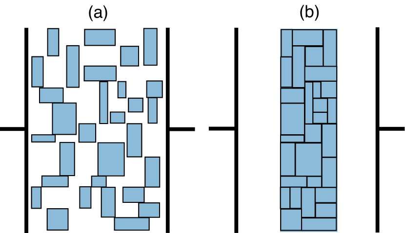
Figure 10: Estimating effective dielectric constants for IDP-water mixtures by consideration of a simple parallel plate capacitor. Here the IDP material is depicted by the shaded areas and water is represented by the white space. The electric capacitance of configurations (a) and (b) are identical irrespective of the dispersion of the IDP material as long as the total width of IDP material is constant over the entire area of the parallel plates (i.e., always constituting $\phi_{m}$ of the distance between the plates). This consideration allows the effective dielectric constant of the mixture in (a) to be determined by standard application of Gauss’ law to (b) under the assumption that the plates are sufficiently large such that edge effects are negligible, as presented in elementary physics textbooks (see, e.g., [114]).

One way to estimate the effective $\epsilon_{r}$ of a mixture of protein (IDP) and water is to consider a pair of infinitely large charged slabs (an electric capacitor) with protein and solvent in between. For a solution in which protein volume ratio is $\phi_{m}$ and water is $1-\phi_{m}$, the electric field $E$ between the two slabs is given by Gauss’ law [114]:

$$\epsilon_{0}E=\phi_{m}\frac{\sigma}{\epsilon_{p}}+(1-\phi_{m})\frac{\sigma}{\epsilon_{w}}\equiv\frac{\sigma}{\epsilon_{\rm eff}},$$ (63)

where $\sigma$ is the charge density on the slabs and $\epsilon_{p},\epsilon_{w}$ are the relative permittivity, respectively, of protein and water. It follows that the effective relative permittivity is given by

$$\epsilon_{\rm eff}(\phi_{m})=\frac{\epsilon_{p}\epsilon_{w}}{\phi_{m}\epsilon_{w}+(1-\phi_{m})\epsilon_{p}}.$$ (64)

We expect this expression to be quite general because for a given $\phi_{m}$, application of Gauss’ law leads to the same $\epsilon_{\rm eff}$, almost – albeit not entirely – irrespective of the configuration of the mixture of the two media, as is illustrated in Fig. 10. An alternative estimate of $\epsilon_{\rm eff}$ is by considering the dipole moments and molecular polarizabilities of water and protein components and apply the Clausius-Mossotti equation [115], which leads to

$$\epsilon_{\rm eff}(\phi_{m})=\frac{1+2[(1-\phi_{m})\gamma_{w}+\phi_{m}\gamma_{p}]}{1-[(1-\phi_{m})\gamma_{w}+\phi_{m}\gamma_{p}]}\;,$$ (65)

where

$$\gamma_{w}\equiv\frac{\epsilon_{w}-1}{\epsilon_{w}+2}\;,\quad\quad\gamma_{p}\equiv\frac{\epsilon_{p}-1}{\epsilon_{p}+2}\;,$$ (66)

are proportional to the molecular polarizabilities of water and protein, respectively. The dependences of $\epsilon_{\rm eff}$ on $\phi_{m}$ estimated from the two approaches are very similar (Fig. 11), buttressing our expectation that the predicted trend is robust. Interestingly, $\epsilon_{\rm eff}$ decreases sharply from that of bulk water for relative small $\phi_{m}$. For instance, $\epsilon_{\rm eff}$ decreases from 80 to $\approx 20$ for $\phi_{m}\approx 20\%$. This effect is significant because according to our RPA+FH model (Fig. 9b), $\phi_{m}$ for the condensed phase of Ddx4 at 60^∘C and [NaCl]= 100mM is $\approx 40\times 10^{-3}\times 236/55.5=17\%$, suggesting that an IDP-concentration-dependent relative permittivity should contribute to a more complete physical account.

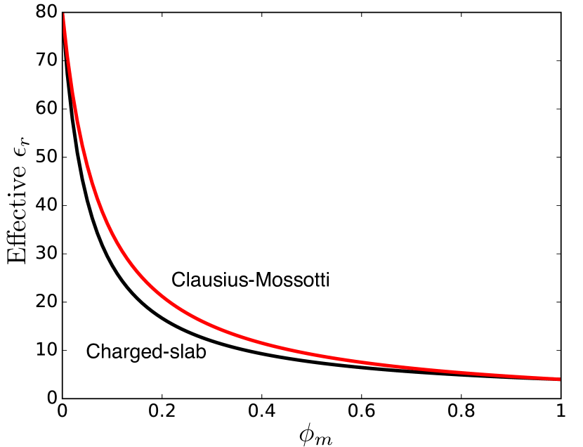
Figure 11: Charged-slab and Clausius-Mossotti models for concentration-dependent relative permittivity. The $\epsilon_{r}(\phi_{m})$ plotted here are the $\epsilon_{\rm eff}$ functions given in Eqs. (64) and (65) for $\epsilon_{p}=4$ and $\epsilon_{w}=80$. The two models predict similar $\phi_{m}$ dependence.

We now incorporate this effect into our RPA theory by replacing $l_{B}$ in Eq. (35) by $l_{B}=e^{2}/(4\pi\epsilon_{0}\epsilon_{r}(\phi_{m})k_{\rm B}T)$, where $\epsilon_{r}(\phi_{m})$ is given by Fig. 11 and, in place of the reduced temperature $T^{*}$ in Eq. (38), define another reduced temperature $T_{0}^{*}$ in terms of vacuum permittivity $\epsilon_{0}$, viz.,

$$T_{0}^{*}\equiv{4\pi\epsilon_{0}k_{\rm B}Tb}/{e^{2}}\;.$$ (67)

In addition, because ${\cal G}$ in Eq. (39) is no longer linear in $\phi_{m}$ because of $\epsilon_{r}(\phi_{m})$, it cannot be used as the last term in the curly brackets of Eq. (39) for the sole purpose of subtracting out unphysical ultraviolet divergences because including a ${\cal G}$ not linear in $\phi_{m}$ would affect phase properties. Consequently, for the case with $\epsilon_{r}(\phi_{m})$, we must derive the dimensionless $f_{\text{el}}$ directly from Eq. (33), yielding

$$f_{\text{el}}=\int\frac{d\tilde{k}\tilde{k}^{2}}{4\pi^{2}}\left\{\frac{1}{\eta}\ln\left[1+\eta{\cal G}_{1}(\tilde{k})\right]-{\cal G}_{2}(\tilde{k})\right\}\;,$$ (68)

where, instead of ${\cal G}$ in Eq. (40), we now have ${\cal G}_{1}$ for the determinant and ${\cal G}_{2}$ for the trace,

$$\!\!{\cal G}_{1}(\tilde{k}) =\frac{4\pi}{\tilde{k}^{2}[1+\tilde{k}^{2}]T_{0}^{*}\epsilon_{r}(\phi_{m})}\left(2\phi_{s}\!+\!\phi_{c}\!+\!\frac{\phi_{m}}{N}\langle\sigma|\hat{G}_{\mathrm{M}}(\tilde{k})|\sigma\rangle\right),$$ (69a)

$$\!\!{\cal G}_{2}(\tilde{k}) =\frac{4\pi}{\tilde{k}^{2}[1+\tilde{k}^{2}]T_{0}^{*}\epsilon_{r}(\phi_{m})}\left(2\phi_{s}\!+\!\phi_{c}\!+\!\frac{\phi_{m}}{N}\sum_{i}|\sigma_{i}|\right)\;.$$ (69b)

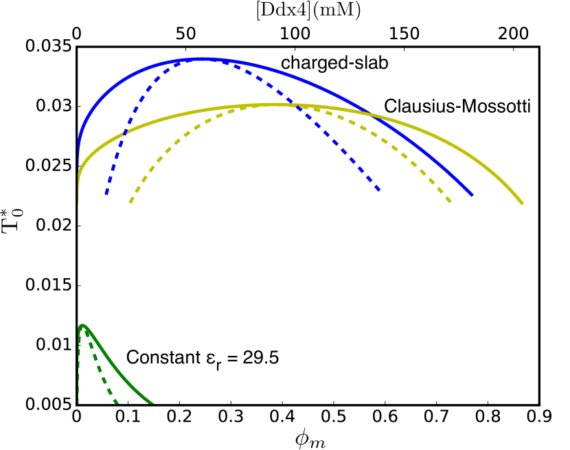
Figure 12: The salt-free phase diagrams of the two $\epsilon_{r}(\phi_{m})$ models in Eqs. (64) and (65) for Ddx4^N1. Solid and dashed lines are, respectively, binodal and spinodal boundaries. IDP and water relative permittivity of $\epsilon_{p}=4$ and $\epsilon_{w}=80$, respectively, are used to calculate $\epsilon_{r}(\phi_{m})$ in both the charged-slab and Clausius-Mossotti models.

Fig. 12 compares the salt-free phase diagrams predicted by this new theory with that obtained using our original RPA theory with $\phi_{m}$-independent $\epsilon_{r}=29.5$. The result indicates that IDP-concentration-dependent $\epsilon_{r}$ can lead to dramatic shifts of phase boundaries. Relative to the constant-$\epsilon_{r}$ model, both $\epsilon_{r}(\phi_{m})$ models have a significantly higher critical temperature and thus a much higher tendency to phase separate. At a qualitative level, the phase-separation enhancing effect of $\epsilon_{r}(\phi_{m})$ is not difficult to understand. As $\epsilon_{r}(\phi_{m})$ decreases with increasing $\phi_{m}$ (Fig. 11), electrostatic interactions favoring formation of a concentrated phase become even stronger with increasing $\phi_{m}$ than if $\epsilon_{r}$ is a constant. This increases the favorability of the concentrated phase, and amounts to a form of many-body electrostatic mechanism that enhances phase transition cooperativity, playing a role similar in effect, though not necessarily in origin, to various many-body mechanisms in cooperative protein folding [116, 117]. This exploratory study has thus demonstrated the potential importance of $\epsilon_{r}(\phi_{m})$-related effects. However, many aspects of these effects, such as possible distance dependence of relative permittivity [108, 118], remain to be investigated. When these issues are addressed in the future, attention should also be paid to the possibility that the tendency for cooperative condensation may be overestimated by using a mean-field concentration $\phi_{m}$ [119], because such cooperativity is likely to be attentuated when constraints from chain connectivity are fully taken into account.

6 Conclusion

In summary, we have presented in some detail a general analytical RPA theory to account for sequence-specific electrostatic effects on polyampholyte phase separation, and demonstrated its utility by applying our theory to Ddx4. Using Ddx4 as an example, we have compared the predicted phase behaviors of RPA and an augmented RPA model with those predicted by FH or OV/DH theories, identifying several salient differences. We have also outlined IDP concentration-dependent relative permittivity as a potentially productive direction for theoretical progress. The predicted phase properties by all of the theories documented here are testable by future experiments.

In the study of IDP phase separation, because direct simulations of multiple-polymer systems are computationally costly, tractable analytical theories are extremely useful for conceptual development, physical insights, and generating new ideas for experiment. However, direct computer simulations of phase separation are indispensable, because they are necessary for checking the validity of the assumptions and approximations in analytical models [120]. RPA assumes uniform densities of counterions and salts. As such it is not expected to be adequate in situations when counterion condensation is significant, such as in the recently observed sequence-dependent coacervation of the Nephrin intracellular domain [36]. Computer simulations and further development of analytical theory, such as the incorporation of formulations that are capable of accounting for effective correlations beyond second order in density fluctuations [89, 121], would be needed in future attempts to address such behaviors.

We deem it fitting to dedicate this paper to the celebration of Professor Vojko Vlachy’s seventieth birthday. Among many of his scientific achievements, Vojko has made seminal contributions to the theory of liquid-liquid phase separation of folded proteins [38] and electrostatic effects in molecular liquids [62]. In view of the recent discovery of polyampholytic IDP phase separation as a major physical basis for membraneless organelles, his pioneering work will no doubt be instructive for future theoretical endeavors to decipher these novel, fascinating biological phenomena. By the same token, experimental techniques that have been applied to study phase separation of folded proteins, such as applications of hydrostatic pressure [122, 123, 124] to investigate phase separation of folded lysozyme [41, 42], may also be brought to bear to enrich our biophysical understanding of sequence-dependent IDP phase separation.

Appendix A The general binodal condition for an arbitrary number of solute components

For a solution with $m$ types of molecules labeled by $i$ with length (number of monomers) $N_{i}$ and monomer size $r_{i}$, and the number of type-$i$ molecules being $n_{i}$, the total number of lattice sites $M=\sum_{k=1}^{m}r_{k}n_{k}N_{k}$ and the free energy per site may be expressed as a function $f(\{\phi_{k}\})$ of the $m-1$ independent densities $\phi_{i}$ defined in Eqs. (3) and (4). Note that there are only $m-1$ independent $\phi_{i}$’s ($i=1,2,\dots,m-1$) because of Eq. (14). The molecule labels are chosen such that $i=m$ for the water solvent.

The chemical potential $\mu_{i}$ of type-$i$ molecules in units of $k_{B}T$ is the derivative of the free energy $F(\{\phi_{k}\})=$ $Mf(\{\phi_{k}\})$ in Eq. (1) with respect to the number $n_{i}$ of type-$i$ molecules [103, 99, 94]:

$$\frac{\mu_{i}}{k_{B}T}= \frac{1}{k_{B}T}\frac{\partial F(\{\phi_{k}\})}{\partial n_{i}}=\frac{\partial Mf(\{\phi_{k}\})}{\partial n_{i}}$$ (70)

$$= \frac{\partial\sum_{k}r_{k}n_{k}N_{k}}{\partial n_{i}}f+M\frac{\partial f(\{\phi_{k}\})}{\partial n_{i}}$$

$$= r_{i}N_{i}f+M\sum_{j=1}^{m-1}\frac{\partial f}{\partial\phi_{j}}\frac{d\phi_{j}}{dn_{i}}$$

$$= r_{i}N_{i}f+M\sum_{j=1}^{m-1}\frac{\partial f}{\partial\phi_{j}}\left(\delta_{ij}\frac{N_{j}}{M}-\frac{n_{j}N_{j}r_{i}N_{i}}{M^{2}}\right)$$

$$= N_{i}\left(r_{i}f+t_{i}f_{i}^{\prime}-r_{i}\sum_{j=1}^{m-1}\phi_{j}f_{j}^{\prime}\right),$$

where $\delta_{ij}$ is the Kronecker symbol, $\delta_{ij}=1$ for $i=j$; $\delta_{ij}=0$ for $i\neq j$, the symbol $t_{i}=1$ for $1\leq i\leq m-1$ and $0$ for $i=m$, and $f_{i}^{\prime}=\partial f/\partial\phi_{i}$ is the first-order derivative of $f$ with respect to $\phi_{i}$. When molecules of type $i$ are carrying charges with valance $z_{i}$ and the Coulomb potential is $\psi^{\alpha}$ in phase $\alpha$, the electrochemical potential

$$\eta_{i}^{\alpha}=\mu_{i}^{\alpha}+z_{i}e\psi^{\alpha}$$ (71)

is the relevant variable for determining the binodal boundary [103]. When the system is demixed to $n_{\rm ph}$ different phases in equilibrium, the chemical, or more generally the electrochemical potentials in all phases have to be identical. In other words,

$$\mu_{i}^{(1)}+z_{i}e\psi^{(1)}=\mu_{i}^{(2)}+z_{i}e\psi^{(2)}=...=\mu_{i}^{(n_{\rm ph})}+z_{i}e\psi^{(n_{\rm ph})}$$ (72)

for all $1\leq i\leq m$ molecule types. This condition provides $m(n_{\rm ph}\!-\!1)$ equations for a total of $n_{\rm ph}(m\!-\!1)$ densities/concentrations $\phi_{i}^{\alpha}$ of all molecule types in all different phases. The maximum number of separated phases $n_{\rm ph,max}$ for a set of environmental conditions such as temperature, pressure, etc. is then given by $m(n_{\rm ph,max}\!-\!1)=n_{\rm ph,max}(m\!-\!1)$, implying $n_{\rm ph,max}=m$ which, as expected, satisfies Gibbs’ phase rule [125]. For $n_{\rm ph}<m$, multiple sets of $\{\phi_{m}^{\alpha}\}$ are allowed, with the sets forming an $(m\!-\!n_{\rm ph})$-dimensional surface in the $(m\!-\!1)$-dimensional $\phi$-space.

We now apply the above general formulation to our polyampholyte system with at most $n_{\rm ph}=2$ separated phases and five different molecule types: polyampholytes with length $N$, size $r_{m}$, and concentration (density) $\phi_{m}$; counterions of size $r_{c}$, concentration $\phi_{c}$; positive and negative salt ions with size $r_{s}$, concentration $\phi_{s\pm}=\phi_{s}$; and water of size $r_{w}$ and $\phi_{w}=$ $(1-r_{m}\phi_{m}-r_{c}\phi_{c}-2r_{s}\phi_{s})/r_{w}$ [Eq. (14)]. Instead of considering only two concentrations $\phi_{m}$ and $\phi_{s}$ as in our discussion of the spinodal condition for our previous Ddx4 model [91] in Eq. (41), here we consider all five concentrations separately for the more general case in which $z_{i}$’s can be different and the system as a whole may not be electrically neutral. Substituting the five molecule types for the $\phi_{i}$’s in Eq. (70) and subtracting the equation for $\mu_{w}$ from other $\eta_{i}$ equations in Eq. (72), we arrive at the following equations for binodal (coexistence) conditions between phases $\alpha$ and $\beta$ ($\alpha,\beta=1,2$), in obvious notation:

$$f_{m}^{\prime\alpha}+\sigma e\psi^{\alpha} =f_{m}^{\prime\beta}+\sigma e\psi^{\beta},$$ (73a)

$$f_{c}^{\prime\alpha}-{\rm sign}(\sigma)e\psi^{\alpha} =f_{c}^{\prime\beta}-{\rm sign}(\sigma)e\psi^{\beta},$$ (73b)

$$f_{s+}^{\prime\alpha}+e\psi^{\alpha} =f_{s+}^{\prime\beta}+e\psi^{\beta},$$ (73c)

$$f_{s-}^{\prime\alpha}-e\psi^{\alpha} =f_{s-}^{\prime\beta}-e\psi^{\beta},$$ (73d)

$$f^{\alpha}-\phi_{m}^{\alpha}f_{m}^{\prime\alpha}-\phi_{c}^{\alpha}f_{c}^{\prime\alpha}- \phi_{s+}^{\alpha}f_{s+}^{\prime\alpha}-\phi_{s-}^{\alpha}f_{s-}^{\prime\alpha}$$

$$=f^{\beta}-\phi_{m}^{\beta}f_{m}^{\prime\beta}-\phi_{c}^{\beta} f_{c}^{\prime\beta}-\phi_{s+}^{\beta}f_{s+}^{\prime\beta}-\phi_{s-}^{\beta}f_{s-}^{\prime\beta},$$ (73e)

where $\sigma=(1/N)\sum_{i=1}^{N}\sigma_{i}$ is the overall average charge density of the polyampholyte. Thus, when the neutrality condition is applied, $\phi_{c}=|\sigma|\phi_{m}$. The above five conditions can be further simplified for our RPA model by evaluating each of the $f^{\prime}$s using the expressions for $s$ and $f_{\rm el}$ in Eqs. (13) and (39), resulting in a free energy that depends only on two concentrations, $f=f(\phi_{m},\phi_{s})$. The corresponding binodal conditions are merged into three equations:

$$\text{Eq.~{}(\ref{eq:df_m})}+\sigma\times\text{Eq.~{}(\ref{eq:df_c})}:$$

$$\qquad\qquad\left.\frac{\partial f(\phi_{m},\phi_{s})}{\partial\phi_{m}}\right|_{\alpha}=\left.\frac{\partial f(\phi_{m},\phi_{s})}{\partial\phi_{m}}\right|_{\beta},$$ (74a)

$$\text{Eq.~{}(\ref{eq:df_sp})}+\text{Eq.~{}(\ref{eq:df_sm})}:$$

$$\qquad\qquad\left.\frac{\partial f(\phi_{m},\phi_{s})}{\partial\phi_{s}}\right|_{\alpha}=\left.\frac{\partial f(\phi_{m},\phi_{s})}{\partial\phi_{s}}\right|_{\beta},$$ (74b)

$$\text{Eq.~{}(\ref{eq:mu_w})}:$$

$$\quad f^{\alpha}-\phi_{m}^{\alpha}\left.\frac{\partial f(\phi_{m},\phi_{s})}{\partial\phi_{m}}\right|_{\alpha}-\phi_{s}^{\alpha}\left.\frac{\partial f(\phi_{m},\phi_{s})}{\partial\phi_{s}}\right|_{\alpha}$$

$$\quad=f^{\beta}-\phi_{m}^{\beta}\left.\frac{\partial f(\phi_{m},\phi_{s})}{\partial\phi_{m}}\right|_{\beta}-\phi_{s}^{\beta}\left.\frac{\partial f(\phi_{m},\phi_{s})}{\partial\phi_{s}}\right|_{\beta}.$$ (74c)

Note that all linear terms of $\phi_{m}$ and $\phi_{s}$ in $(\phi_{m},\phi_{i})$ have no effect in Eq. (74) because they only add an equal constant to both sides of Eqs. (74a) and (74b) and they cancel out by themselves on each side of Eq. (74c).

The conditions in Eq. (74) are equations for the common tangent of free energy function $f(\phi_{m},\phi_{s})$ at two points $\alpha=(\phi_{m}^{\alpha},\phi_{s}^{\alpha})$ and $\beta=(\phi_{m}^{\beta},\phi_{s}^{\beta})$. Because there are only three equations in Eq. (74) for the four variables $\phi_{m}^{\alpha}$, $\phi_{m}^{\beta}$, $\phi_{s}^{\alpha}$, and $\phi_{s}^{\beta}$, the common-tangent pair $(\alpha,\beta)$ is not unique determined. A given temperature $T^{*}$ is consistent with a series of $(\alpha,\beta)$. These common-tangent sets constitute a closed contour on the $\phi_{m}$–$\phi_{s}$ surface as the binodal boundary [104]. A system with a set of original bulk concentrations $O=(\phi_{m}^{0},\phi_{s}^{0})$ inside the contour will phase separate to two regions with concentrations $(\phi_{m}^{\alpha},\phi_{s}^{\alpha})$, $(\phi_{m}^{\beta},\phi_{s}^{\beta})$ such that $O,\alpha,\beta$ are on the same common tangent. In other words, a fourth equation for solving a unique set of $(\alpha,\beta)$ is provided by the initial concentrations.

Appendix B Critical points of strictly alternating polyampholytes in the $N\to\infty$ limit

In the limit of $N\to\infty$, the parameters $A$ and $B$ in Eq. (57) can be expressed as

$$A= A_{r}(\sigma)\sigma^{3/2}T^{*-2},$$ (75a)

$$B= B_{r}(\sigma)\sigma^{3/2}T^{*-3},$$ (75b)

where $A_{r}$ and $B_{r}$ are functions of $\sigma$ via the following integrals,

$$A_{r}(\sigma)= \sqrt{\frac{8}{3}}\int_{0}^{\infty}\!\!\frac{dk^{\prime}}{k^{\prime 2}(1+6\sigma k^{\prime 2})^{2}}\left(\frac{1-e^{-k^{\prime 2}}}{1+e^{-k^{\prime 2}}}\right)^{2}$$ (76a)

$$B_{r}(\sigma)= \sqrt{\frac{128}{27}}\pi\int_{0}^{\infty}\!\!\frac{dk^{\prime}}{k^{\prime 4}(1+6\sigma k^{\prime 2})^{3}}\left(\frac{1-e^{-k^{\prime 2}}}{1+e^{-k^{\prime 2}}}\right)^{3}.$$ (76b)

As $\sigma\to 0$, $A_{r}\to 1.374$ and $B_{r}\to 1.187$, as has been shown in Eqs. (56) and (59). For general $\sigma\leq 1$, $A_{r}$ and $B_{r}$ become much smaller because of the short range cutoff $(1+6\sigma k^{\prime 2})$.

To self-consistently solve the critical point, we calculate the derivatives of free energy $f=-s+f_{\text{el}}^{\infty}$,

$$\left.\frac{\partial^{2}f}{\partial\phi_{m}^{2}}\right|_{\phi_{m}=\phi_{\mathrm{cr}},T^{*}=T^{*}_{\mathrm{cr}}}=0\;\text{\ and\ }\left.\frac{\partial^{3}f}{\partial\phi_{m}^{3}}\right|_{\phi_{m}=\phi_{\mathrm{cr}},T^{*}=T^{*}_{\mathrm{cr}}}=0,$$ (77)

with the $f_{\text{el}}^{\infty}$ in Eq. (57), yielding

$$\frac{1}{N\phi_{\mathrm{cr}}}+\frac{1}{1-\phi_{\mathrm{cr}}}-A_{r}\frac{\sigma^{3/2}}{T^{*2}_{\mathrm{cr}}}+B_{r}\frac{\sigma^{3/2}}{T^{*3}_{\mathrm{cr}}}\phi_{\mathrm{cr}}=0\;,$$ (78a)

$$-\frac{1}{N\phi_{\mathrm{cr}}^{2}}+\frac{1}{(1-\phi_{\mathrm{cr}})^{2}}+B_{r}\frac{\sigma^{3/2}}{T^{*3}_{\mathrm{cr}}}=0\;.$$ (78b)

We first substitute Eq. (78b) into Eq. (78a) for the $B_{r}$ term to obtain

$$A_{r}\frac{\sigma^{3/2}}{T^{*2}_{\mathrm{cr}}}=\frac{2}{N\phi_{\mathrm{cr}}}+\frac{1}{1-\phi_{\mathrm{cr}}}-\frac{\phi_{\mathrm{cr}}}{(1-\phi_{\mathrm{cr}})^{2}}\;,$$ (79)

then we simultaneously express $1/T^{*}_{\mathrm{cr}}$ by Eqs. (78b) and (79) to arrive at the following two equalities:

$$\frac{1}{T^{*}_{\mathrm{cr}}}= \left[\left(\frac{2}{N\phi_{\mathrm{cr}}}+\frac{1}{1-\phi_{\mathrm{cr}}}-\frac{\phi_{\mathrm{cr}}}{(1-\phi_{\mathrm{cr}})^{2}}\right)\frac{1}{\sigma^{3/2}A_{r}(\sigma)}\right]^{1/2}$$ (80)

$$= \left[\left(\frac{1}{N\phi_{\mathrm{cr}}^{2}}-\frac{1}{(1-\phi_{\mathrm{cr}})^{2}}\right)\frac{1}{\sigma^{3/2}B_{r}(\sigma)}\right]^{1/3}\;.$$

Now $\phi_{\mathrm{cr}}$ can first be solved numerically using the second equality. Then $T^{*}_{\mathrm{cr}}$ can be solved by substituting the $\phi_{\mathrm{cr}}$ value into the first equality.

$\sigma$	$\phi_{\mathrm{cr}}$ (s-a)	$\phi_{\mathrm{cr}}$ (num)	$T^{*}_{\mathrm{cr}}$ (s-a)	$T^{*}_{\mathrm{cr}}$ (num)
0.025	$0.00669$	$0.00909$	0.02833	0.03260
0.05	$0.00880$	0.01126	0.04148	0.04601
0.1	0.01111	0.01361	0.05634	0.06091
0.2	0.01354	0.01604	0.07136	0.07578

Table 1: The critical point parameters $\phi_{\mathrm{cr}}$ and $T^{*}_{\mathrm{cr}}$ of $N=240$ strictly alternating polyampholytes, calculated by the semi-analytic method (s-a) in Eq. (80) and the numerical method (num) described in Sec. 2.3. The deviation of the semi-analytic results from the numerical results increases as $\sigma$ decreases.

We provide in Table 1 the critical points of $N=240$ strictly alternating polyampholytes calculated semi-analytically by pursuing numerical solutions to the analytic Eq. (80) and compare them with the numerical results computed by the method described in Sec. 2.3. For $\sigma=0.2$, the present semi-analytic (s-a) method provides a reasonable approximation, with 20% and 6% deviations in $\phi_{\mathrm{cr}}$ and $T^{*}_{\mathrm{cr}}$, respectively. Both approaches yielded $\phi_{\mathrm{cr}}$ values that are much smaller than the $1/\sqrt{240}=0.06$ value one might otherwise expect from FH. Interestingly, however, their $T^{*}_{\mathrm{cr}}$ are close to the FH prediction of $T^{*}_{\mathrm{cr}}=0.03$ – $0.06$ for the different $\sigma$ values tested.

References

References

- Kendrew et al. [1958] J. C. Kendrew, G. Bodo, H. M. Dintzis, R. G. Parrish, H. Wyckoff, A three-dimensional model of the myoglobin molecule obtained by x-ray analysis, Nature 181 (1958) 662–666.
- Uversky et al. [2000] V. N. Uversky, J. R. Gillespie, A. L. Fink, Why are natively unfolded proteins unstructured under physiologic conditions?, Proteins 41 (3) (2000) 415–427.
- Dunker et al. [2001] A. K. Dunker, J. D. Lwason, C. J. Brown, R. M. Williams, P. Romero, J. S. Oh, C. J. Oldfield, A. M. Campen, C. R. Ratliff, K. W. Hipps, J. Ausio, M. S. Nissen, R. Reeves, C. H. Kang, C. R. Kissinger, R. W. Bailey, M. D. Griswold, M. Chiu, E. C. Garner, Z. Obradovic, Intrinsically disordered proteins, J. Molecular Graphics & Modelling 19 (1) (2001) 26–59.
- Tompa [2001] P. Tompa, Intrinsically unstructured proteins, Trends Biochem. Sci. 27 (10) (2001) 527–533.
- Gunasekaran et al. [2003] K. Gunasekaran, C. J. Tsai, S. Kumar, D. Zanuy, R. Nussinov, Extended disordered proteins: targeting function with less scaffod, Trends Biochem. Sci. 28 (2) (2003) 81–85.
- Dyson and Wright [2005] H. J. Dyson, P. E. Wright, Intrinsically unstructured proteins and their functions, Nature Rev. Mol. Cell Biol. 6 (3) (2005) 197–208.
- Tompa [2012] P. Tompa, Intrinsically unstructured proteins: a 10-year recap, Trends Biochem. Sci. 37 (2012) 509–516.
- Marsh et al. [2012] J. A. Marsh, S. A. Teichmann, J. D. Forman-Kay, Probing the diverse landscape of protein flexibility and binding, Curr. Opin. Struct. Biol. 22 (2012) 643–650.
- Forman-Kay and Mittag [2013] J. D. Forman-Kay, T. Mittag, From sequence and forces to structure, function, and evolution of intrinsically disordered proteins, Structure 21 (9) (2013) 1492–1499.
- van der Lee et al. [2014] R. van der Lee, M. Buljan, B. Lang, R. J. Weatheritt, G. W. Daughdrill, A. K. Dunker, M. Fuxreiter, J. Gough, J. Gsponer, D. T. Jones, et al., Classification of intrinsically disordered regions and proteins, Chem. Rev. 114 (13) (2014) 6589–6631.
- Liu and Huang [2014] Z. Liu, Y. Huang, Advantages of proteins being disordered, Protein Sci. 23 (5) (2014) 539–550.
- Chen et al. [2015] T. Chen, J. Song, H. S. Chan, Theoretical perspectives on nonnative interactions and intrinsic disorder in protein folding and binding, Curr. Opin. Struct. Biol. 30 (2015) 32–42.
- Das et al. [2015] R. K. Das, K. M. Ruff, R. V. Pappu, Relating sequence encoded information to form and function of intrinsically disordered proteins, Curr. Opin. Struct. Biol. 32 (2015) 102–112.
- Wright and Dyson [2015] P. E. Wright, H. J. Dyson, Intrinsically disordered proteins in cellular signalling and regulation, Nat. Rev. Mol. Cell Biol. 16 (2015) 18–29.
- Csizmok et al. [2016] V. Csizmok, A. V. Follis, R. W. Kriwacki, J. D. Forman-Kay, Dynamic protein interaction networks and new structural paradigms in signaling, Chem. Rev. 116 (11) (2016) 6424–6462.
- Wu and Fuxreiter [2016] H. Wu, M. Fuxreiter, The structure and dynamics of higher-order assemblies: Amyloids, signalosomes, and granules, Cell 165 (5) (2016) 1055–1066.
- Bah et al. [2015] A. Bah, R. M. Vernon, Z. Siddiqui, M. Krzeminski, R. Muhandiram, C. Zhao, N. Sonenberg, L. E. Kay, J. D. Forman-Kay, Folding of an intrinsically disordered protein by phosphorylation as a regulatory switch, Nature 519 (2015) 106–109.
- Tompa and Fuxreiter [2008] P. Tompa, M. Fuxreiter, Fuzzy complexes: Polymorphism and structural disorder in protein-protein interactions, Trends Biochem. Sci. 33 (2008) 2–8.
- Nash et al. [2001] P. Nash, X. Tang, S. Orlicky, Q. Chen, F. B. Gertler, M. D. Mendenhall, F. Sicheri, T. Pawson, M. Tyers, Multisite phosphorylation of a CDK inhibitor sets a threshold for the onset of DNA replication, Nature 414 (2001) 514–521.
- Borg et al. [2007] M. Borg, T. Mittag, T. Pawson, M. Tyers, J. D. Forman-Kay, H. S. Chan, Polyelectrostatic interactions of disordered ligands suggest a physical basis for ultrasensitivity, Proc. Natl. Acad. Sci. USA 104 (2007) 9650–9655.
- Mittag et al. [2010] T. Mittag, J. Marsh, A. Grishaev, S. Orlicky, H. Lin, F. Sicheri, M. Tyers, J. D. Forman-Kay, Structure/function implications in a dynamic complex of the intrinsically disordered Sic1 with the Cdc4 subunit of an SCF ubiquitin ligase, Structure 18 (2010) 494–506.
- Brangwynne et al. [2009] C. P. Brangwynne, C. R. Eckmann, D. S. Courson, A. Rybarska, C. Hoege, J. Gharakhani, F. Jülicher, A. A. Hyman, Germline P granules are liquid droplets that localize by controlled dissolution/condensation, Science 324 (2009) 1729–1732.
- Dundr and Misteli [2010] M. Dundr, T. Misteli, Biogenesis of nuclear bodies, Cold Spring Harb. Perspect. Biol. 2 (12) (2010) a000711.
- Li et al. [2012] P. Li, S. Banjade, H.-C. Cheng, S. Kim, B. Chen, L. Guo, M. Llaguno, J. V. Hollingsworth, D. S. King, S. F. Banani, P. S. Russo, Q. Jiang, B. T. Nixon, M. K. Rosen, Phase transitions in the assembly of multivalent signalling proteins, Nature 483 (2012) 336–340.
- Kato et al. [2012] M. Kato, T. W. Han, S. Xie, K. Shi, X. Du, L. C. Wu, H. Mirzaei, E. J. Goldsmith, J. Longgood, J. Pei, N. V. Grishin, D. E. Frantz, J. W. Schneider, S. Chen, L. Li, M. R. Sawaya, D. Eisenberg, R. Tycko, S. L. McKnight, Cell-free formation of RNA granules: Low complexity sequence domains form dynamic fibers within hydrogels, Cell 149 (2012) 753–767.
- Lee et al. [2013] C. F. Lee, C. P. Brangwynne, J. Gharakhani, A. A. Hyman, F. Jülicher, Spatial organization of the cell cytoplasm by position-dependent phase separation, Phys. Rev. Lett. 111 (8) (2013) 088101.
- Hyman et al. [2014] A. A. Hyman, C. A. Weber, F. Jülicher, Liquid-liquid phase separation in biology, Annu. Rev. Cell. Dev. Biol. 30 (2014) 39–58.
- Toretsky and Wright [2014] J. A. Toretsky, P. E. Wright, Assemblages: Functional units formed by cellular phase separation, J. Cell. Biol. 206 (2014) 579–588.
- Wang et al. [2014] J. T. Wang, J. Smith, B. C. Chen, H. Schmidt, D. Rasoloson, A. Paix, L. B. G, D. Calidas, E. Betzig, G. Seydoux, Regulation of RNA granule dynamics by phosphorylation of serine-rich, intrinsically disordered proteins in C. elegans, eLife 3 (2014) e04591.
- Nott et al. [2015] T. J. Nott, E. Petsalaki, P. Farber, D. Jervis, E. Fussner, A. Plochowietz, T. D. Craggs, D. P. Bazett-Jones, T. Pawson, J. D. Forman-Kay, A. J. Baldwin, Phase transition of a disordered nuage protein generates environmentally responsive membraneless organelles, Mol. Cell. 57 (5) (2015) 936–947.
- Elbaum-Garfinkle et al. [2015] S. Elbaum-Garfinkle, Y. Kim, K. Szczepaniak, C. C.-H. Chen, C. R. Eckmann, S. Myong, C. P. Brangwynne, The disordered P granule protein LAF-1 drives phase separation into droplets with tunable viscosity and dynamics, Proc. Natl. Acad. Sci. USA 112 (23) (2015) 7189–7194.
- Kroschwald et al. [2015] S. Kroschwald, S. Maharana, D. Mateju, L. Malinovska, E. Nuske, I. Poser, D. Richter, S. Alberti, Promiscuous interactions and protein disaggregases determine the material state of stress-inducible RNP granules, eLife 4 (2015) e06807.
- Brangwynne et al. [2015] C. P. Brangwynne, P. Tompa, R. V. Pappu, Polymer physics of intracellular phase transitions, Nat. Phys. 11 (2015) 899–904.
- Nott et al. [2016] T. J. Nott, T. D. Craggs, A. J. Baldwin, Membraneless organelles can melt nucleic acid duplexes and act as biomolecular filters, Nature Chem. 8 (2016) 569–575.
- Banani et al. [2016] S. F. Banani, A. M. Rice, W. B. Peeples, Y. Lin, S. Jain, R. Parker, M. K. Rosen, Compositional control of phase-separated cellular bodies, Cell 166 (2016) 651–663.
- Pak et al. [2016] C. W. Pak, M. Kosno, A. S. Holehouse, S. B. Padrick, A. Mittal, R. Ali, A. A. Yunus, D. R. Liu, R. V. Pappu, M. K. Rosen, Sequence determinants of intracellular phase separation by complex coacervation of a disordered protein, Mol. Cell 63 (2016) 72–85.
- Knowles et al. [2014] T. P. J. Knowles, M. Vendruscolo, C. M. Dobson, The amyloid state and its association with protein misfolding diseases, Nat. Rev. Mol. Cell Biol. 15 (2014) 384–396.
- Vlachy et al. [1993] V. Vlachy, H. W. Blanch, J. M. Prausnitz, Liquid-liquid phase separations in aqueous solutions of globular proteins, AlChE J. 39 (1993) 215–223.
- Sear [1999] R. P. Sear, Phase behavior of a simple model of globular proteins, J. Chem. Phys. 111 (10) (1999) 4800–4806.
- Tavares and Prausnitz [2004] F. W. Tavares, J. M. Prausnitz, Analytical calculation of phase diagrams for solutions containing colloids or globular proteins, Colloid Polym. Sci. 282 (6) (2004) 620–632.
- Schroer et al. [2011] M. A. Schroer, J. Markgraf, D. C. F. Wieland, C. J. Sahle, J. Möller, M. Paulus, M. Tolan, R. Winter, Nonlinear pressure dependence of the interaction potential of dense protein solutions, Phys. Rev. Lett. 106 (1) (2011) 178102.
- Möller et al. [2014] J. Möller, S. Grobelny, J. Schulze, S. Bieder, A. Steffen, M. Erlkamp, M. Paulus, M. Tolan, R. Winter, Reentrant liquid-liquid phase separation in protein solutions at elevated hydrostatic pressures, Phys. Rev. Lett. 112 (2) (2014) 028101.
- Prausnitz [2015] J. Prausnitz, The fallacy of misplaced concreteness, Biophys. J. 108 (3) (2015) 453–454.
- Kastelic et al. [2015] M. Kastelic, Y. V. Kalyuzhnyi, B. Hribar-Lee, K. A. Dill, V. Vlachy, Protein aggregation in salt solutions, Proc. Natl. Acad. Sci. USA (2015) 6766–6770.
- Dill [1990] K. A. Dill, Dominant forces in protein folding, Biochemistry 29 (1990) 7133–7155.
- Dosztanyi et al. [2005] Z. Dosztanyi, V. Csizmok, P. Tompa, I. Simon, IUPred: web server for the prediction of intrinsically unstructured regions of proteins based on estimated energy content, Bioinformatics 21 (16) (2005) 3433–3434.
- Xue et al. [2010] B. Xue, R. L. Dunbrack, R. W. Williams, A. K. Dunker, V. N. Uversky, PONDR-Fit: A meta-predictor of intrinsically disordered amino acids, Biochim. Biophys. Acta 1804 (4) (2010) 966–1010.
- Uversky [2015] V. N. Uversky, The intrinsic disordered alphabet. III. Dual personality of serine, Intrinsically Disordered Proteins 3 (1) (2015) 1–21.
- Higgs and Joanny [1991] P. G. Higgs, J.-F. Joanny, Theory of polyampholyte solutions, J. Chem. Phys. 94 (2) (1991) 1543–1554.
- Dobrynin et al. [2004] A. V. Dobrynin, R. H. Colby, M. Rubinstein, Polyampholytes, J. Polym. Sci. Part B Polym. Phys. 42 (2004) 3513–3538.
- Müller-Späth et al. [2010] S. Müller-Späth, A. Soranno, V. Hirschfeld, H. Hofmann, S. Rüegger, L. Reymond, D. Nettels, B. Schuler, Charge interactions can dominate the dimensions of intrinsically disordered proteins, Proc. Natl. Acad. Sci. USA 107 (33) (2010) 14609–14614.
- Das and Pappu [2013] R. K. Das, R. V. Pappu, Conformations of intrinsically disordered proteins are influenced by linear sequence distributions of oppositely charged residues, Proc. Natl. Acad. Sci. USA 110 (33) (2013) 13392–13397.
- Song et al. [2015] J. Song, G. N. Gomes, C. C. Gradinaru, H. S. Chan, An adequate account of excluded volume is necessary to infer compactness and asphericity of disordered proteins by Förster resonance energy transfer, J. Phys. Chem. B 119 (2015) 15191–15202.
- Quiroz and Chilkoti [2015] F. G. Quiroz, A. Chilkoti, Sequence heuristics to encode phase behaviour in intrinsically disordered protein polymers, Nat. Mater. 14 (11) (2015) 1164–1171.
- Ruff et al. [2015] K. M. Ruff, T. S. Harmon, R. V. Pappu, CAMELOT: A machine learning approach for coarse-grained simulations of aggregation of block-copolymeric protein sequences, J. Chem. Phys. 143 (2) (2015) 243123.
- Huggins [1941] M. L. Huggins, Solutions of long chain compounds, J. Chem. Phys. 9 (1941) 440.
- Flory [1942] P. J. Flory, Thermodynamics of high polymer solutions, J. Chem. Phys. 10 (1942) 51–61.
- Flory [1953] P. J. Flory, Principles of Polymer Chemistry, Cornell University Press, 1953.
- Chan and Dill [1991] H. S. Chan, K. A. Dill, Polymer principles in protein structure and stability, Annu. Rev. Biophys. Biophys. Chem. 20 (1991) 447–490.
- Debye and E [1923] P. Debye, H. E, Zur Theorie der Elektrolyte. I. Gefrierpunktserniedrigung und verwandte erscheinungen (The theory of electrolytes. I. Lowering of freezing point and related phenomena), Physikalische Zeitschrift 24 (1923) 185–206.
- Wright [2007] M. R. Wright, An Introduction to Aqueous Electrolyte Solutions, John Wiley & Sons, 2007.
- Vlachy [1999] V. Vlachy, Ionic effects beyond Poisson-Boltzmann theory, Annu. Rev. Phys. Chem. 50 (1999) 145–165.
- Derjaguin and Landau [1941] B. Derjaguin, L. Landau, Theory of the stability of strongly charged lyophobic sols and of the adhesion of strongly charged particles in solutions of electrolytes, Acta physicochim. URSS 14 (6) (1941) 633–662.
- Verwey and Overbeek [1948] E. J. W. Verwey, J. T. G. Overbeek, Theory of the Stability of Lyophobic Colloids, Elsevier, Amsterdam, 1948.
- Friedman [1985] H. L. Friedman, A course in statistical mechanics, Prentice-Hall, 1985.
- Wertheim [1986] M. S. Wertheim, Fluids with highly directional attractive forces. III. Multiple attraction sites, J. Stat. Phys. 42 (3) (1986) 459–476.
- Blum [1977] L. Blum, Theory of electrified interfaces, J. Phys. Chem. 81 (2) (1977) 136–147.
- Wertheim [1963] M. S. Wertheim, Exact solution of the Percus-Yevick integral equation for hard spheres, Phys. Rev. Lett. 10 (8) (1963) 321–323.
- de Gennes [1979] P.-G. de Gennes, Scaling Concepts in Polymer Physics, Cornell University Press, 1979.
- Borue and Erukhimovich [1988] V. Y. Borue, I. Y. Erukhimovich, A statistical theory of weakly charged polyelectrolytes: fluctuations, equation of state and microphase separation, Macromolecules 21 (1988) 3240–3249.
- Rescic et al. [1990] J. Rescic, V. Vlachy, A. D. J. Haymet, Highly asymmetric electrolytes: beyond the hypernetted chain integral equation, J. Am. Chem. Soc. 112 (1990) 3398–3401.
- Borue and Erukhimovich [1990] V. Y. Borue, I. Y. Erukhimovich, A statistical theory of globular polyelectrolyte complexes, Macromolecules 23 (1990) 3625–3632.
- Gonzalez-Mozuelos and Olvera de la Cruz [1994] P. Gonzalez-Mozuelos, M. Olvera de la Cruz, Random phase approximation for complex charged systems: Application to copolyelectrolytes (polyampholytes), J. Chem. Phys. 100 (1) (1994) 507–517.
- Mahdi and Olvera de la Cruz [2000] K. A. Mahdi, M. Olvera de la Cruz, Phase diagrams of salt-free polyelectrolyte semidilute solutions, Macromolecules 33 (2000) 7649–7654.
- Bernard and Blum [2000] O. Bernard, L. Blum, Thermodynamics of a model for flexible polyelectrolytes in the binding mean spherical approximation, J. Chem. Phys. 112 (1) (2000) 7227–7237.
- Jiang et al. [2001] J. W. Jiang, L. Blum, O. Bernard, J. M. Prausnitz, Thermodynamic properties and phase equilibria of charged hard sphere chain model for polyelectrolyte solutions, Mol. Phys. 99 (1) (2001) 1121–1128.
- Wittmer et al. [1993] J. Wittmer, A. Johner, J. F. Joanny, Random and alternating polyampholytes, EPL 24 (1993) 263–268.
- Dobrynin [1995] A. V. Dobrynin, Fluctuation theory of charged AB-random copolymers, J. Phys. II 5 (8) (1995) 1241–1253.
- Jiang et al. [2006] J. Jiang, J. Feng, H. Liu, Y. Hu, Phase behavior of polyampholytes from charged hard-sphere chain model, J. Chem. Phys. 124 (14) (2006) 144908–144908.
- Cheong and Panagiotopoulos [2005] D. W. Cheong, A. Z. Panagiotopoulos, Phase behaviour of polyampholyte chains from grand canonical Monte Carlo simulations, Mol. Phys. 103 (2005) 3031–3044.
- Overbeek and Voorn [1957] J. T. G. Overbeek, M. J. Voorn, Phase separation in polyelectrolyte solutions. Theory of complex coacervation, J. Cell. Compar. Physl. 49 (1957) 7–26.
- Schmitt et al. [1998] C. Schmitt, C. Sanchez, S. Desobry-Banon, J. Hardy, Structure and technofunctional properties of protein-polysaccharide complexes: a review, Critical reviews in food science and nutrition 38 (8) (1998) 689–753.
- Weinbreck et al. [2003] F. Weinbreck, R. de Vries, P. Schrooyen, C. G. de Kruif, Complex coacervation of whey proteins and gum arabic, Biomacromolecules 4 (2) (2003) 293–303.
- Schmitt and Turgeon [2011] C. Schmitt, S. L. Turgeon, Protein/polysaccharide complexes and coacervates in food systems, Advances in colloid and interface science 167 (1-2) (2011) 63–70.
- Stigter et al. [1991] D. Stigter, D. O. V. Alonso, K. A. Dill, Protein stability: Electrostatics and compact denatured states, Proc. Natl. Acad. Sci. USA 88 (1991) 4176–4178.
- Dill and Stigter [1995] K. A. Dill, D. Stigter, Modeling protein stability as heteropolymer collapse, Adv. Protein. Chem. 46 (1995) 59–104.
- Wertheim [1984] M. S. Wertheim, Fluids with highly directional attractive forces. I. Statistical thermodynamics, Journal of Statistical Physics 35 (1) (1984) 19–34.
- Zhang and Cremer [2009] Y. Zhang, P. S. Cremer, The inverse and direct Hofmeister series for lysozyme, Proc. Natl. Acad. Sci. USA 106 (36) (2009) 15249–15253.
- Sawle and Ghosh [2015] L. Sawle, K. Ghosh, A theoretical method to compute sequence dependent configurational properties in charged polymers and proteins, J. Chem. Phys. 143 (2015) 085101.
- Vovk et al. [2016] A. Vovk, C. Gu, M. G. Opferman, L. E. Kapinos, R. Y. H. Lim, R. D. Coalson, D. Jasnow, A. Zilman, Simple biophysics underpins collective conformations of the intrinsically disordered proteins of the Nuclear Pore Complex, eLife 5 (2016) e10785.
- Lin et al. [2016] Y.-H. Lin, J. D. Forman-Kay, H. S. Chan, Sequence-specific polyampholyte phase separation in membraneless organelles, Phys. Rev. Lett., accepted for publication; available as arXiv1605.09019 [q-bio.BM] .
- Liang et al. [1994] L. Liang, W. Diehl-Jones, P. Lasko, Localization of vasa protein to the Drosophila pole plasm is independent of its RNA-binding and helicase activities, Development 120 (5) (1994) 1201–1211.
- Dill et al. [1989] K. A. Dill, D. O. V. Alonso, K. Hutchinson, Thermal stabilities of globular proteins, Biochemistry 28 (1989) 5439–5449.
- Chan and Dill [1994] H. S. Chan, K. A. Dill, Solvation: Effects of molecular size and shape, J. Chem. Phys. 101 (1994) 7007–7026.
- Ermoshkin and Olvera de la Cruz [2004] A. V. Ermoshkin, M. Olvera de la Cruz, Gelation in strongly charged polyelectrolytes, J. Polym. Sci. Part B Polym. Phys. 42 (2004) 766–776.
- Doi and Edwards [1986] M. Doi, S. F. Edwards, The Theory of Polymer Dynamics, Clarendon Press, Oxford, UK, 1986.
- Ermoshkin and Olvera de la Cruz [2003a] A. V. Ermoshkin, M. Olvera de la Cruz, Polyelectrolytes in the presence of multivalent ions: gelation versus segregation, Phys. Rev. Lett. 90 (12) (2003a) 125504.
- Ermoshkin and Olvera de la Cruz [2003b] A. V. Ermoshkin, M. Olvera de la Cruz, A modified random phase approximation of polyelectrolyte solutions, Macromolecules 36 (20) (2003b) 7824–7832.
- Grosberg and Khokhlov [1994] A. Y. Grosberg, A. R. Khokhlov, Statistical Physics of Macromolecules, AIP: Woodbury, NY, 1994.
- Itzykson and Zuber [1980] C. Itzykson, J.-B. Zuber, Quantum Field Theory, McGraw-Hill, Inc., New York, 1980.
- Voorn [1956a] M. J. Voorn, Complex coacervation. II. Thermodynamic calculations on a specific model, with application to two component systems, Recl. Trav. Chim. Pays-Bas 75 (4) (1956a) 405–426.
- Rubinstein and Colby [2003] M. Rubinstein, R. H. Colby, Polymer Physics, Oxford University Press, Oxford, UK, 2003.
- Voorn [1956b] M. J. Voorn, Complex coacervation. I. General theoretical considerations, Recl. Trav. Chim. Pays-Bas 75 (3) (1956b) 317–330.
- Voorn [1956c] M. J. Voorn, Complex coacervation. III. Thermodynamic calculations on three-component systems, Recl. Trav. Chim. Pays-Bas 75 (4) (1956c) 427–446.
- Voorn [1956d] M. J. Voorn, Complex coacervation: IV. Thermodynamic calculations on four-component systems, Recl. Trav. Chim. Pays-Bas 75 (8) (1956d) 925–937.
- Pitera et al. [2001] J. W. Pitera, M. Falta, W. F. van Gunsteren, Dielectric properties of proteins from simulation: the effects of solvent, ligands, pH, and temperature, Biophys. J 80 (6) (2001) 2546–2555.
- Warshel et al. [2006] A. Warshel, P. K. Sharma, M. Kato, W. W. Parson, Modeling electrostatic effects in proteins, Biochim. Biophys. Acta 1764 (11) (2006) 1647–1676.
- Leach [1996] A. R. Leach, Molecular Modeling. Principles and Applications (p.170), Addison Wesley Longman Limited, Singapore, 1996.
- Ma and Dougherty [1997] J. C. Ma, D. A. Dougherty, The cation- interaction, Chem. Rev. 97 (1997) 1303–1324.
- Meyer et al. [2003] E. A. Meyer, R. K. Castellano, F. Diederich, Interactions with aromatic rings in chemical and biological recognition, Angew. Chem. Int. Ed. Engl. 42 (11) (2003) 1210–1250.
- Song et al. [2013] J. Song, S. C. Ng, P. Tompa, K. A. W. Lee, H. S. Chan, Polycation- interactions are a driving force for molecular recognition by an intrinsically disordered oncoprotein family, PLoS Comput. Biol. 9 (2013) e1003239.
- Schmidt and Görlich [2015] H. B. Schmidt, D. Görlich, Nup98 FG domains from diverse species spontaneously phase-separate into particles with nuclear pore-like permselectivity, eLife 4 (2015) e04251.
- Vernon et al. [2016] R. M. Vernon, P. J. Farber, J. D. Forman-Kay, Planar interactions: an overlooked feature in proteins and relevance to phase separation, (in preparation) .
- Grant and Phillips [1975] I. S. Grant, W. R. Phillips, Electromagnetism (pp.53–58), John Wiley & Sons Ltd., Chichester, U.K., 1975.
- Jackson [1975] J. D. Jackson, Classical Electrodynamics, 2nd ed (pp.154–155), John Wiley & Sons, Inc., New York, 1975.
- Badasyan et al. [2008] A. Badasyan, Z. Liu, H. S. Chan, Probing possible downhill folding: Native contact topology likely places a significant constraint on the folding cooperativity of proteins with residues, J. Mol. Biol. 384 (2008) 512–530.
- Chan et al. [2011] H. S. Chan, Z. Zhang, S. Wallin, Z. Liu, Cooperativity, local-nonlocal coupling, and nonnative interactions: Principles of protein folding from coarse-grained models, Annu. Rev. Phys. Chem. 62 (2011) 301–326.
- Shen and Freed [2005] M. Y. Shen, K. F. Freed, A simple method for faster nonbonded force evaluations, J. Comput. Chem. 26 (2005) 691–698.
- Wang and Wang [2014] R. Wang, Z.-G. Wang, Theory of polymer chains in poor solvent: Single-chain structure, solution thermodynamics, and point, Macromolecules 47 (2014) 4094–4102.
- Orkoulas et al. [2003] G. Orkoulas, S. K. Kumar, A. Z. Panagiotopoulos, Monte Carlo study of coulombic criticality in polyelectrolytes, Phys. Rev. Lett. 90 (4) (2003) 048303.
- Muthukumar [1996] M. Muthukumar, Double screening in polyelectrolyte solutions: Limiting laws and crossover formulas, J. Chem. Phys. 105 (12) (1996) 5183–5199.
- Royer and Winter [2011] C. A. Royer, R. Winter, Protein hydration and volumetric properties, Curr. Opin. Colloid Interface Sci. 16 (2011) 568–571.
- Silva et al. [2014] J. L. Silva, A. C. Oliveira, T. C. R. G. Vieira, G. A. P. de Oliveira, M. C. Suarez, D. Foguel, Protein hydration and volumetric properties, Chem. Rev. 114 (2014) 7239–7267.
- Dias and Chan [2014] C. L. Dias, H. S. Chan, Pressure-dependent properties of elementary hydrophobic interactions: Ramifications for activation properties of protein folding, J. Phys. Chem. B 118 (2014) 7488–7509.
- Atkins and de Paula [2009] P. Atkins, J. de Paula, Physical Chemistry, W H Freeman & Co., NY, 9 edn., 2009.