ASYMPTOTIC BEHAVIOR OF THE CURVES
IN THE FUCIK SPECTRUM

Abstract.

In this work we study the asymptotic behavior of the curves of the Fučík spectrum for weighted second order linear ordinary differential equations. We prove a Weyl type asymptotic behavior of the hyperbolic type curves in the spectrum in terms of some integrals of the weights. We present an algorithm which computes the intersection of the Fučík spectrum with rays through the origin, and we compare their values with the asymptotic ones.

1. Introduction

We are interested here in the shape of the curves in the Fučík spectrum for the following problem

(1) $$\begin{cases}-u^{\prime\prime}=\alpha\,m(x)u^{+}-\beta\,n(x)u^{-}\qquad x\in(0,L)\\ u(0)=u(L)=0,\end{cases}$$

where $(\alpha,\beta)\in\mathbb{R}^{2}_{+}$, and the functions $m$, $n\in C[0,L]$ are positive and bounded below by some positive constant $c$. As usual, given a function $u$ we denote $u^{\pm}=\max\{0,\pm u\}$ the positive and negative parts of $u$.

This problem was introduced in the ’70s by Dancer and Fučík (see [7, 10]), for constant weights $m=n$. They were interested in problems with jumping non-linearities, and they obtained for $m$, $n\equiv 1$ that (1) has a nontrivial solution corresponding to $(\alpha,\beta)$ if and only if:

• $\alpha=(\pi/L)^{2}$, for any $\beta\in\mathbb{R}$,

• $\beta=(\pi/L)^{2}$, for any $\alpha\in\mathbb{R}$,

• $(\alpha,\beta)\in\mathbb{R}^{2}_{+}$ belong to the following families of hyperbolic-like curves $\mathcal{C}_{k}$,

  $$\mathcal{C}_{k}: \quad\frac{k\pi}{2L\sqrt{\alpha}}+\frac{k\pi}{2L\sqrt{\beta}}=1,\qquad k\in\mathbb{N}\mbox{ even}$$

  $$\mathcal{C}_{k}^{+}: \quad\frac{(k+1)\pi}{2L\sqrt{\alpha}}+\frac{(k-1)\pi}{2L\sqrt{\beta}}=1,\qquad k\in\mathbb{N}\mbox{ odd}$$

  $$\mathcal{C}_{k}^{-}: \quad\frac{(k-1)\pi}{2L\sqrt{\alpha}}+\frac{(k+1)\pi}{2L\sqrt{\beta}}=1,\qquad k\in\mathbb{N}\mbox{ odd.}$$

The existence of similar curves in the spectrum was proved later for non-constant weights $m\not\equiv n$ by Rynne in [14] , together with several properties about simplicity of zeros, monotonicity of the eigenvalues respect to the pair of weights, continuity and differentiability of the curves, and the asymptotic behavior of the curves when $\alpha$ or $\beta\to\infty$. For sign-changing weights, similar results were obtained by Alif and Gossez, and they can be found in [1, 2].

All these results were generalized for half-linear differential equations involving the one dimensional $p-$Laplacian operator,

(2) $$\begin{cases}-(|u^{\prime}|^{p-2}u^{\prime})^{\prime}=\alpha m(x)|u^{+}|^{p-2}u^{+}-\beta n(x)|u^{-}|^{p-2}u^{-}\qquad x\in(0,L)\\ u(0)=u(L)=0\end{cases}$$

with different boundary conditions, see for instance Section 6.3.3 in [8] for the constant coefficient case, or [4, 6] where indefinite weights $m$, $n$ and different boundary conditions were considered.

By using shooting arguments Rynne proved that the spectrum of problem (1) can be described as an union of curves

$$\Sigma:=\mathcal{C}_{0}^{\pm}\cup\bigcup_{k\in\mathbb{N}}\mathcal{C}_{k}^{\pm}.$$

The curves $\mathcal{C}_{0}^{\pm}$ are called the trivial curves since the eigenfunctions does not changes signs, we can write $\mathcal{C}_{0}^{+}=\{\lambda_{1}^{m}\}\times\mathbb{R}$, $\mathcal{C}_{0}^{-}=\mathbb{R}\times\{\lambda_{1}^{n}\}$, where $\lambda_{1}^{s}$ denotes the first eigenvalue of problem

(3) $$\begin{cases}-u^{\prime\prime}=\lambda s(x)u,&\qquad x\in(0,L)\\ u(0)=u(L)=0.&\end{cases}$$

The curve $\mathcal{C}_{k}^{+}$ (resp. $\mathcal{C}_{k}^{-}$) correspond to pairs $(\alpha,\beta)$ with a nontrivial solution having $k$ internal zeros and positive (resp. negative) slope at the origin. Let us observe that now we have two curves for $k$ even, in the constant coefficient case both curves coincide but this is not true for general weights.

The curves $\mathcal{C}_{k}^{+}$ are not known for general weights $m$, $n$, and only its limit behavior as $\alpha$ or $\beta\to\infty$ is known. This behavior is related to the sequence of eigenvalues $\{\lambda_{k}^{s}\}_{k\in\mathbb{N}}$ of problem (3), and we have that:

• When $k\in\mathbb{N}$ is even, the curves $\mathcal{C}_{k}^{\pm}$ are asymptotic to the line $\mathbb{R}\times\lambda_{k/2}^{n}$ as $\alpha\to\infty$; and to the line $\lambda_{k/2}^{m}\times\mathbb{R}$ as $\beta\to\infty$.

• When $k\in\mathbb{N}$ is odd, $\mathcal{C}_{k}^{+}$ is asymptotic to the line $\mathbb{R}\times\lambda_{(k-1)/2}^{n}$, and $\mathcal{C}_{k}^{-}$ is asymptotic to the line $\mathbb{R}\times\lambda_{(k+1)/2}^{n}$, as $\alpha\to+\infty$.

• When $k\in\mathbb{N}$ is odd, $\mathcal{C}_{k}^{-}$ is asymptotic to the line $\mathbb{R}\times\lambda_{(k+1)/2}^{n}$, and $\mathcal{C}_{k}^{-}$ is asymptotic to the line $\mathbb{R}\times\lambda_{(k-1)/2}^{n}$, as $\alpha\to+\infty$.

Although in some cases the curves $\mathcal{C}_{k}^{+}$ and $\mathcal{C}_{k}^{-}$ can coincide in one or more points, in this work we will think of them as different curves. That is, we will consider as different two eigenfunctions if one of them starts with positive slope, and the other one start with negative slope.

Our main objective in this work is to give a description of the asymptotic behavior of the curves $\mathcal{C}_{k}^{\pm}$. Quantitative bounds of the Fučík spectrum are by far less common in the literature, and the qualitative description states that they are $C^{1}$ curves. By using the ideas in [12] it is possible to enclose with an hyperbolic like curve the region of the plane containing the Fučík eigenpairs whose corresponding eigenfunctions have $k$ nodal domains. Here, we give an explicit asymptotic description of the curves together with an error term, in the spirit of Weyl’s asymptotic of the Laplacian eigenvalues.

In order to state our results, let us introduce some notations. We denote by $\mathcal{K}_{\theta}$ a symmetric region in the first quadrant (with respect to the line $x=y$) between two rays through the origin forming an angle $\theta\in(0,\pi/2)$. Moreover, $f(k)\sim g(k)$ as $k\to\infty$ means that $\lim_{k\to\infty}f(k)/g(k)=1$.

In order to improve the asymptotic estimates, we must impose an additional condition on the weights, related to the Morrey-Campanato space $L^{\gamma,1}(0,L)$:

Definition 1.1.

Given $\gamma>0$, we say that the function $m$ satisfies the $\gamma$-condition if $m$ is continuous and there exists two positive constants $m_{1}$, $m_{2}$ such that $0<m_{1}\leq m\leq m_{2}<\infty$ and $m\in L^{\gamma,1}(0,L)$, the Morrey-Companato space of functions in $L^{1}(0,L)$ satisfying

$$\int_{I}|m-m_{I}|\leq C|I|^{\gamma}$$

for any $I\subset(0,L)$, where $C$ is a fixed constant and

$$m_{I}=\frac{1}{|I|}\int_{I}m(x)dx$$

is the mean value of $m$ in $I$.

Observe that, when $m$ is Hölder continuous of order $r>0$ and bounded away from zero, then it satisfies the $\gamma-$condition for $0\leq\gamma\leq 1+r/2$.

Our first result correspond to the case $m=n$:

Theorem 1.2.

Let $\Sigma$ be the Fučík spectrum of problem (1), and let $m\equiv n$ be a continuous function in $[0,L]$, bounded below by some some positive constant. Let $(\alpha_{k}^{\pm},\beta_{k}^{\pm})\in\mathcal{C}_{k}^{\pm}$. Given some fixed angle $\theta\in(0,\pi/2)$, the curves $\mathcal{C}_{k}^{\pm}$ have the following asymptotic behavior in the region $\mathcal{K}_{\theta}$

$$1\sim\frac{\pi k}{2}\left(\frac{(\alpha_{k}^{\pm})^{-\frac{1}{2}}+(\beta_{k}^{\pm})^{-\frac{1}{2}}}{\int_{0}^{L}m^{\frac{1}{2}\,dx}}\right)$$

as $k\to\infty$.

For different weights $m$ and $n$ we have:

Theorem 1.3.

Let $\Sigma$ be the Fučík spectrum of problem (1) where $m$, $n$ are continuous functions in $[0,L]$, bounded below by some some positive constant. Let $(\alpha_{k}^{\pm},\beta_{k}^{\pm})\in\mathcal{C}_{k}^{\pm}$. Given some fixed angle $\theta\in(0,\pi/2)$, the curves $\mathcal{C}_{k}^{\pm}$ have the following asymptotic behavior in the region $\mathcal{K}_{\theta}$

$$1\sim\frac{\pi k}{2}\left(\int_{0}^{L}\Big{(}(\alpha_{k}^{\pm}m)^{-\frac{1}{2}}+(\beta_{k}^{\pm}n)^{-\frac{1}{2}}\Big{)}^{-1}\,dx\right)^{-1}$$

as $k\to\infty$. Moreover, if $\big{(}m^{-\frac{1}{2}}+(nt)^{-\frac{1}{2}}\big{)}^{-1}$ satisfies the $\gamma$-condition for some $\gamma>1$, then for all $\delta\in[\frac{1}{\gamma},1]$, we have

$$1=\frac{\pi k}{2}\left(\int_{0}^{L}\Big{(}(\alpha_{k}^{\pm}m)^{-\frac{1}{2}}+(\beta_{k}^{\pm}n)^{-\frac{1}{2}}\Big{)}^{-1}\,dx\right)^{-1}+O(k^{\delta})$$

as $k\to\infty$.

Remark 1.4.

When $\alpha_{k}^{\pm}=\beta_{k}^{\pm}$, and $m=n$, the pair of curves intersect at an eigenvalue $\lambda_{k}$ of the Sturm-Liouville problem (3) with $s\equiv m$, and we recover the well known asymptotic formula of Weyl,

$$\lambda_{k}\sim\left(\frac{\pi k}{\int_{0}^{L}m^{\frac{1}{2}}\,dx}\right)^{2}.$$

We divide the proof of Theorem 1.3 in several steps. The first step is to fix a line $(\lambda,t\lambda)$ in the first quadrant and to estimate the number of intersections with the curves in $\Sigma$ as a function of $\lambda$. To this end, we need to study the eigenvalue problem

(4) $$\begin{cases}-u^{\prime\prime}=\lambda(m(x)u^{+}-tn(x)u^{-})&\qquad x\in[0,L]\\ u(0)=u(L)=0.&\end{cases}$$

These eigenvalues are related to the half-eigenvalues studied for instance in [4, 11]. Observe that only a positive multiple of a solution is itself a solution corresponding to the same eigenvalue, if a negative multiple is a solution too, we will count this as a double eigenvalue.

From the description of the Fučík spectrum of problem (1), the spectrum of problem (4) consists in a double sequence

(5) $$0<\lambda_{1,t}^{\pm}<\lambda_{2,t}^{\pm}<\lambda_{3,t}^{\pm}<\cdots<\lambda_{2k-1,t}^{\pm}<\lambda_{2k,t}^{\pm}\cdots\nearrow\infty$$

for each fixed $t>0$. Each eigenvalue $\lambda_{2,t}^{\pm}$ has a unique associated eigenfunction, normalized by $\pm u^{\prime}(0)=1$. The eigenfunction corresponding to $\lambda_{k,t}^{\pm}$ has precisely $k$ nodal domains on $(0,L)$, and $k+1$ zeros in $[0,L]$. Moreover, for $t=1$ we have $\lambda^{+}_{k,1}=\lambda_{k,1}^{-}$.

We introduce the spectral counting function $N(\lambda,t,(0,L))$, defined as

$$N(\lambda,t,(0,L))=\#\{k:\lambda_{k,t}^{+}(0,L)\leq\lambda\}+\#\{k:\lambda_{k,t}^{-}(0,L)\leq\lambda\}.$$

We emphasize the dependence of the eigenvalues on the interval, since in order to count these eigenvalues, we use a bracketing argument comparing them with the eigenvalues in subintervals. However, since the problem has no variational structure, we cannot use the Dirichlet-Neumann bracketing of Courant [5]. Moreover, since the Sturmian oscillation theory does not hold for Fučík eigenvalues, and it is not true that between two zeros of an eigenfunction there is at least a zero of any eigenfunction corresponding to a higher eigenvalue, we cannot use a different bracketing based on the number of zeros nor the Sturm-Liouville theory that can be found in [13], and we need to prove the following theorem:

Theorem 1.5.

Let $N(\lambda,t,(0,L))$ be the spectral counting function of problem (4) where $m$, $n$ are continuous functions in $[0,L]$, bounded below by some some positive constant. Let $c\in(0,L)$. Then for any fixed $t>0$,

$$N(\lambda,t,(0,L))=N(\lambda,t,(0,c))+N(\lambda,t,(c,L))+O(1)$$

when $\lambda\to\infty$.

From Theorem 1.5 we derive the following Weyl type result:

Theorem 1.6.

Let $N(\lambda,t,(0,L))$ be the spectral counting function on $(0,L)$ of problem (4), where $m$, $n$ are continuous functions in $[0,L]$, bounded below by some some positive constant. For any fixed $t>0$,

$$N(\lambda,t,(0,L))=\frac{4\sqrt{\lambda}}{\pi}\int_{0}^{L}\big{(}m^{-\frac{1}{2}}+(nt)^{-\frac{1}{2}}\big{)}^{-1}\,dx+o(\sqrt{\lambda})$$

as $\lambda\to\infty$.

Finally, let us show that the error term in Theorem 1.6 can be improved for more regular weights satisfying the $\gamma$-condition introduced in Definition 1.1, following the ideas in [9].

Theorem 1.7.

Suppose that $\big{(}m^{-\frac{1}{2}}+(nt)^{-\frac{1}{2}}\big{)}^{-1}$ satisfies the $\gamma$-condition for some $\gamma>1$. Then for each $t>0$ fixed and for all $\delta\in[\frac{1}{\gamma},1]$, we have

$$N(\lambda,(0,L))=\frac{4\sqrt{\lambda}}{\pi}\int_{0}^{L}\big{(}m^{-\frac{1}{2}}+(nt)^{-\frac{1}{2}}\big{)}^{-1}\,dx+O(\lambda^{\delta/2}).$$

Let us observe that the arguments here can be easily modified and applied to problem (2), and also for other homogeneous boundary conditions. However, those arguments are strongly dependent on the one dimensional nature of the problem, and we cannot expect an easy generalization to higher dimensional problems where, on the other hand, several strange phenomena can occur.

The paper is organized as follows. In Section 2 we review some necessary facts about the eigenvalues and we prove the bracketing argument in Theorem 1.5. We prove Theorems 1.3, 1.6 and 1.7 in Section 3. In Section 4 we present some numerical experiments.

2. A fixed line

Let us study the distribution of the intersection between $\Sigma$ and a line $\beta=t\alpha$ through the origin for a fixed $t>0$. Let us call $\alpha=\lambda$ and $\beta=t\alpha=t\lambda$, and let us describe the spectrum of problem (4).

We consider first the case of constant weights $m$ and $n$. Hence, the intersection $\Sigma\cap\{(\lambda,t\lambda):\lambda>0\}$ can be computed explicitly:

Lemma 2.1.

Let $\{\lambda_{k}^{\pm}\}_{k\in\mathbb{N}}$ be the eigenvalues of (4) with constant weights in $(0,L)$. Then, for each fixed $t>0$, we have

(6) $$\begin{split}&(\lambda_{k,t}^{\pm})^{\frac{1}{2}}=\frac{k\pi}{2L}\left(m^{-\frac{1}{2}}+(nt)^{-\frac{1}{2}}\right),\qquad\qquad\qquad\qquad k\mbox{ even}\\ &(\lambda_{k,t}^{+})^{\frac{1}{2}}=\frac{\pi}{2L}\left((k+1)m^{-\frac{1}{2}}+(k-1)(nt)^{-\frac{1}{2}}\right),\qquad k\mbox{ odd}\\ &(\lambda_{k,t}^{-})^{\frac{1}{2}}=\frac{\pi}{2L}\left((k-1)m^{-\frac{1}{2}}+(k+1)(nt)^{-\frac{1}{2}}\right),\qquad k\mbox{ odd.}\end{split}$$

We omit the proof since it follows from the explicit formula for the Fučík eigenvalues with constant weights given in the Introduction.

We are interested now in the spectral counting function $N(\lambda,t,(0,L))$ for any fixed $t>0$. In order to prove Theorem 1.5, we review the characterization of the eigenvalues in terms of the Prüfer angle.

We introduce two auxiliary functions $\rho$, $\varphi$ and we propose the following Prüfer type transformation

(7) $$\begin{cases}u(x)&=\sqrt{\lambda m(x)}\sin(\varphi(x))^{+}-\sqrt{\lambda tn(x)}\sin(\varphi(x))^{-},\\ u^{\prime}(x)&=\rho(x)\cos(\varphi(x)),\end{cases}$$

and an straightforward computation shows that $\rho(x)$ and $\varphi(x)$ satisfy the system of ordinary differential equations

(8) $$\varphi^{\prime}(x)=\begin{cases}\sqrt{\lambda m(x)}+\frac{1}{2}\frac{m^{\prime}(x)}{m(x)}\cos(\varphi(x))\sin(\varphi(x))&\qquad\mbox{if }\sin(\varphi(x))\geq 0\\ \sqrt{\lambda n(x)}+\frac{1}{2}\frac{n^{\prime}(x)}{n(x)}\cos(\varphi(x))\sin(\varphi(x))&\qquad\mbox{if }\sin(\varphi(x))<0,\end{cases}$$

(9) $$\rho^{\prime}(x)=\begin{cases}\frac{1}{2}\frac{m^{\prime}(x)}{m(x)}\rho(x)\sin^{2}(\varphi(x))&\qquad\mbox{if }\sin(\varphi(x))\geq 0\\ \frac{1}{2}\frac{n^{\prime}(x)}{n(x)}\rho(x)\sin^{2}(\varphi(x))&\qquad\mbox{if }\sin(\varphi(x))<0.\end{cases}$$

Now, a shooting argument enable us to compute the eigenvalues since the corresponding eigenfunctions have a given number of zeros. The zeros of $u$ depend on the zeros of $\sin(\varphi(x))$ since the function $\rho$ is strictly positive. Whenever $\varphi(x)$ is an integer multiple of $\pi$, we have $\varphi^{\prime}(x)>0$. Hence, we have the following characterization of the eigenvalues:

$$\lambda_{k}^{+}=\min\{\lambda\,:\,\varphi(\lambda,0)=0,\varphi(\lambda,L)=k\pi\},\qquad\quad$$

$$\lambda_{k}^{-}=\min\{\lambda\,:\,\varphi(\lambda,0)=\pi,\varphi(\lambda,L)=(k+1)\pi\}.$$

The next Lemma is a version of the well-known Sturm’s Comparison Theorem for the half-eigenvalues of (4), and it is an easy consequence of the previous characterization of eigenvalues in terms of the Prüfer transformation, see Theorem 5.3 in [14].

Lemma 2.2.

Let $m_{i}$, $n_{i}$ $i=1,2$ positive and continuous weights such that $m_{1}\geq m_{2}$ and $n_{1}\geq n_{2}$, and let us call $\lambda_{k,t}^{\pm}(m_{i},n_{i})$ the corresponding half-eigenvalues of problem (4). Then $\lambda_{k,t}(m_{1},n_{1})\leq\lambda_{k,t}(m_{2},n_{2})$.

As a consequence, we have the following bound for the Fučík eigenvalues with two weights in terms of the eigenvalues of a weighted problem:

Lemma 2.3.

Let $m$, $n$ be positive and continuous weights and let us call $\lambda_{k,t}^{\pm}(m,n)$ the corresponding half-eigenvalues of problem (4). Then $\lambda_{k,t}(m,n)\leq\mu_{k}$, where $\mu_{k}$ is the $k$-th eigenvalue of the problem:

$$-v^{\prime\prime}=\mu\frac{mnt}{m+nt}v,$$

with zero Dirichlet boundary conditions.

Proof.

We have the following inequalities,

$$\frac{mnt}{m+nt}\leq\frac{mnt}{nt}=m$$

$$\frac{mnt}{m+nt}\leq\frac{mnt}{m}=nt$$

and by Lemma 2.2, we have

$$\lambda_{k,t}^{\pm}(m,n)\leq\lambda_{k,t}^{\pm}\left(\frac{mnt}{m+nt},\frac{mnt}{m+nt}\right),$$

which coincides with $\mu_{k}$. ∎

A critical step in the proof of Theorem 1.5 is the following Lemma, which is a consequence of the Sturmian oscillation theory in classical eigenvalue problems:

Lemma 2.4.

Let $\lambda>\lambda_{k,t}^{+}$ (resp., $\lambda>\lambda_{k,t}^{-}$), and let $\varphi(\lambda,x)$ corresponding to a solution of equation (4) satisfying $u(0)=0$ and $u(0^{+})>0$ (resp., $u(0^{+})<0$). Then $\varphi(\lambda,L)>k\pi$ (resp., $\varphi(\lambda,L)>(k+1)\pi$).

Proof.

Let us consider only the case $u(0^{+})>0$, the other one is similar. Let us denote by $\{0,x_{1},\cdots,x_{k-1},L\}$ the zeros of an eigenfunction corresponding to $\lambda_{k,t}^{+}$.

In the first nodal domain $(0,x_{1})$ we can apply the classical Sturmian theory, so the solution $u$ has a first zero at $0$, and another zero $y_{1}<x_{1}$.

Now, the next zero $y_{2}$ must be located before $x_{2}$, or the second nodal domain starting in $y_{1}$ strictly contains the interval $(x_{1},x_{2})$. However, this is not possible, since $\lambda_{k}^{+}<\lambda$ and the Sturm-Liouville theory implies that $u$ must have a zero between $x_{1}$ and $x_{2}$.

In much the same way, the nodal domain starting at $y_{2}<x_{2}$ cannot contain the full interval $(x_{2},x_{3})$, and applying this argument repeatedly, we obtain that $y_{k}<L$.

Finally, since $\varphi$ cannot decrease at a multiple of $\pi$, we have $\varphi(\lambda,L)>k\pi$ and the Lemma is proved. ∎

Proof of Theorem 1.5.

Let us consider the following auxiliary eigenvalue problems in $(0,c)$ and $(c,L)$, with the original boundary conditions in $0$ and $L$, and Neumann boundary conditions at $c$:

(10) $$\begin{split}\begin{cases}&-u^{\prime\prime}=\mu(m(x)u^{+}-tn(x)u^{-})\qquad x\in(0,c)\\ &u(0)=u^{\prime}(c)=0,\end{cases}\end{split}$$

(11) $$\begin{split}\begin{cases}&-u^{\prime\prime}=\mu(m(x)u^{+}-tn(x)u^{-})\qquad x\in(c,L)\\ &u^{\prime}(c)=u(L)=0.\end{cases}\end{split}$$

We have two double sequences of eigenvalues $\{\mu_{k,t}^{\pm}(0,c)\}_{k\geq 1}$, $\{\mu_{k,t}^{\pm}(c,L)\}_{k\geq 1}$ corresponding to problems (10) and (11).

Let us fix $\lambda$, and there exists some integer $n$ such that

$$\lambda_{n-1,t}^{-}<\lambda_{n,t}^{+}\leq\lambda<\lambda_{n+1,t}^{+}<\lambda_{n+2,t}^{-}.$$

Moreover, let us note that there exist an even integer $j$ such that $\mu_{j,t}^{+}(0,c)\leq\lambda<\mu_{j+2,t}^{+}(0,c)$, and an integer $h$ such that $\mu_{h,t}^{+}(c,L)\leq\lambda<\mu_{h+1,t}^{+}(c,L)$.

Observe that $\lambda_{n,t}^{+}\leq\lambda$ does not implies $\lambda_{n,t}^{-}\leq\lambda$, and by using similar arguments in all the cases we obtain the following bounds:

(12) $$\begin{split}2n-1&\leq N(\lambda,t,(0,L))\leq 2n+1\\ 2j-1&\leq N(\lambda,t,(0,c))\leq 2(j+1)+1\\ 2h-1&\leq N(\lambda,t,(c,L))\leq 2h+1.\end{split}$$

We claim now that

$$-9\leq N(\lambda,t,(0,L)))-N(\lambda,t,(0,c))-N(\lambda,t,(c,L))\leq 11.$$

The eigenfunctions corresponding to $\mu_{j,t}^{+}(0,c)$ and $\mu_{h,t}^{+}(c,L)$ have $j+1$ zeros in $[0,c]$ and $h+1$ in $[c,L]$ respectively. Since both solutions have a zero at $c$, we have $j+h+1$ zeros in $[0,L]$.

Now, let $\mu=\max\{\mu_{j,t}^{+}(0,c),\mu_{h,t}^{+}(c,L)\}$, and let us solve equation (8) for $\lambda=\mu$. We start the shooting at $0$ if $\mu=\mu_{j,t}^{+}(0,c)$ with $\varphi(\mu,0)=0$, or we solve it backwards starting from $L$ if $\mu=\mu_{h,t}^{+}(c,L)$ with $\varphi(\mu,L)=\pi$. Hence, Lemma 2.4 implies that this solution has at least $i+j+1$ zeros in $[0,L]$.

We compare now this solution with the one corresponding to $\lambda_{n+1,t}^{+}$ (if $\mu=\mu_{j,t}^{+}(0,c)$) or the one corresponding to $\lambda_{n+2,t}^{-}$ (if $\mu=\mu_{h,t}^{+}(c,L)$). In both cases, we get

(13) $$j+h+1\leq n+3.$$

We can obtain another inequality starting with the eigenfunctions corresponding to $\mu_{j+2,t}^{+}(0,c)$ and $\mu_{h+1,t}^{+}(c,L)$, they have $j+3$ zeros in $[0,c]$ and $h+2$ in $[c,L]$, respectively. Hence, we have $j+h+4$ zeros in $[0,L]$. Comparing as before, by choosing now $\mu=\min\{\mu_{j+2,t}^{+}(0,c),\mu_{h+1,t}^{+}(c,L)\}$, the corresponding solution has lower than $j+h+4$ zeros, and the zeros of the eigenfunctions corresponding to $\lambda_{n,t}^{+}$ or $\lambda_{n-1,t}^{-}$ can be bounded below by $n$. So, we get

(14) $$n\leq j+h+4.$$

Therefore, inequalities (13) and (14), together with inequalities (12) implies the claim, and the proof is finished. ∎

3. The proof of the main theorems

In this section we prove Theorems 1.3, 1.6 and 1.7. For convenience, we prove first lower and upper bounds for the eigenvalue counting function, and we introduce the following notation: given two functions $m$, $n$ we denote

$$d_{t}(m,n)=m^{-\frac{1}{2}}+(nt)^{-\frac{1}{2}}.$$

Lemma 3.1.

Let $t>0$ be fixed, and let $\{\lambda_{k,t}^{\pm}\}_{k\in\mathbb{N}}$ be the eigenvalues of problem (4) in $(0,L)$ and suppose that $\underline{m}\leq m\leq\overline{m}$, $\underline{n}\leq n\leq\overline{n}$. Then

$$N(\lambda,t,(0,L))\geq\frac{4\sqrt{\lambda}L}{\pi}\big{(}d_{t}(\underline{m},\underline{n})\big{)}^{-1}-1,$$

$$N(\lambda,t,(0,L))\leq\frac{4\sqrt{\lambda}L}{\pi}\big{(}d_{t}(\overline{m},\overline{n})\big{)}^{-1}+2.$$

Proof.

The proof follows as a consequence of the monotonicity of eigenvalues respect to the weight in Lemma 2.2. For $k$ even we have that

(15) $$\frac{k^{2}\pi^{2}}{4L^{2}}\big{(}d_{t}(\overline{m},\overline{n})\big{)}^{2}\leq\lambda_{k,t}^{\pm}\leq\frac{k^{2}\pi^{2}}{4L^{2}}\big{(}d_{t}(\underline{m},\underline{n}\big{)}\big{)}^{2}.$$

Consequently, if we consider only the even curves,

$$\#\{\lambda_{k,t}^{\pm}\leq\lambda,k\textrm{ even}\} \geq\#\Big{\{}k:\frac{k^{2}\pi^{2}}{4L^{2}}d_{t}(\underline{m},\underline{n})^{2}\leq\lambda,k\mbox{ even}\Big{\}}$$

$$\#\{\lambda_{k,t}^{\pm}\leq\lambda,k\textrm{ even}\} \leq\#\Big{\{}k:\frac{k^{2}\pi^{2}}{4L^{2}}d_{t}(\overline{m},\overline{n})^{2}\leq\lambda,k\mbox{ even}\Big{\}}.$$

Hence, denoting by $\lfloor{x}\rfloor$ the largest integer not greater than $x$, we have

$$\#\{\lambda_{k,t}^{\pm}\leq\lambda,k\textrm{ even}\} \geq\left\lfloor\frac{2\sqrt{\lambda}L}{\pi}d_{t}(\underline{m},\underline{n})^{-1}\right\rfloor$$

$$\#\{\lambda_{k,t}^{\pm}\leq\lambda,k\textrm{ even}\} \leq\left\lfloor\frac{2\sqrt{\lambda}L}{\pi}d_{t}(\overline{m},\overline{n})^{-1}\right\rfloor.$$

The lower bound follows by bounding $\lfloor{x}\rfloor\geq x-1$, and the other one follows since $\lfloor{x}\rfloor\leq x$ and there is a pair of odd curves between two pairs of even curves. The Lemma is proved. ∎

We are ready to prove Theorem 1.6. Essentially, we split $(0,L)$ in finitely many intervals, and then we apply Theorem 1.5 and Lemma 3.1.

Proof of Theorem 1.6.

Let us split $(0,L)$ as

$$(0,L)=\cup_{1\leq j\leq J}I_{j},$$

where $I_{j}\cap I_{k}=\emptyset$, and $|I_{j}|=L/J=\eta$. We define

$$\underline{m}_{j}=\inf_{x\in I_{j}}m(x),\quad\overline{m}_{j}=\sup_{x\in I_{j}}m(x).$$

Since $m$ and $n$ are continuous functions they are Riemann integrable, and given any $\varepsilon>0$, we can choose $\eta>0$ such that

$$\sum_{j=1}^{J}\eta\big{(}(\underline{m}_{j})^{-\frac{1}{2}}+(\underline{n}_{j}t)^{-\frac{1}{2}}\big{)}^{-1}\geq\int_{0}^{L}\big{(}m^{-\frac{1}{2}}+(nt)^{-\frac{1}{2}}\big{)}^{-1}\,dx-\varepsilon,$$

$$\sum_{j=1}^{J}\eta\big{(}(\overline{m}_{j})^{-\frac{1}{2}}+(\overline{n}_{j}t)^{-\frac{1}{2}}\big{)}^{-1}\leq\int_{0}^{L}\big{(}m^{-\frac{1}{2}}+(nt)^{-\frac{1}{2}}\big{)}^{-1}\,dx+\varepsilon.$$

From Theorem 1.5 we have that

$$N(\lambda,t,(0,L))=\sum_{j=1}^{J}N(\lambda,t,I_{j})+O(J),$$

and Lemma 3.1 implies

$$\sum_{j=1}^{J}N(\lambda,t,I_{j}) \leq\sum_{j=1}^{J}\frac{4\eta\sqrt{\lambda}}{\pi}\big{(}(\overline{m}_{j})^{-\frac{1}{2}}+(\overline{n}_{j}t)^{-\frac{1}{2}}\big{)}^{-1}+O(J)$$

$$=\frac{4\sqrt{\lambda}}{\pi}\Big{(}\int_{0}^{L}\big{(}m^{-\frac{1}{2}}+(nt)^{-\frac{1}{2}}\big{)}^{-1}\,dx+\varepsilon\Big{)}+O(J)$$

$$\sum_{j=1}^{J}N(\lambda,t,I_{j}) \geq\sum_{j=1}^{J}\frac{4\eta\sqrt{\lambda}}{\pi}\big{(}(\underline{m}_{j})^{-\frac{1}{2}}+(\underline{n}_{j}t)^{-\frac{1}{2}}\big{)}^{-1}-O(J)$$

$$=\frac{4\sqrt{\lambda}}{\pi}\Big{(}\int_{0}^{L}\big{(}m^{-\frac{1}{2}}+(nt)^{-\frac{1}{2}}\big{)}^{-1}\,dx-\varepsilon\Big{)}-O(J)$$

and the proof is complete. ∎

Let us prove now Theorem 1.7.

Proof of Theorem 1.7.

Let $0<\eta<\eta_{1}<0$ be fixed, and let us split $(0,L)=\cup_{1\leq j\leq J}I_{j}$ as before, where $I_{j}\cap I_{k}=\emptyset$, $|I_{j}|=L/J=\eta$.

Let us define, for $1\leq i\leq J$

$$\varphi(\lambda)=\frac{2\sqrt{\lambda}}{\pi}\int_{0}^{L}d_{t}(m,n),\qquad\varphi(\lambda,I_{j})=\frac{2\eta\sqrt{\lambda}d_{I_{j}}}{\pi}$$

where $d_{I_{j}}=|I_{j}|^{-1}\int_{I_{j}}d_{t}(m,n)$.

From Theorem 1.5 we obtain

(16) $$\sum_{j=1}^{J}N(\lambda,t,I_{j},d_{t})-\varphi(\lambda)-O(J)\leq N(\lambda,t,(0,L),d_{t})-\varphi(\lambda)$$

(17) $$N(\lambda,t,(0,L),d_{t})-\varphi(\lambda)\leq\sum_{j=1}^{J}N(\lambda,t,I_{j},d_{t})-\varphi(\lambda)+O(J).$$

Let us bound the left hand side of inequality (16); we have

$$\begin{split}\sum_{j=1}^{J}N(\lambda,t,I_{j},d_{t})-\varphi(\lambda)&\leq\sum_{j=1}^{J}N(\lambda,t,I_{j},d_{I_{j}})-\varphi(\lambda,I_{j})\\ &\quad+\sum_{j=1}^{J}\varphi(\lambda,I_{j})-\varphi(\lambda)\\ &\quad+\sum_{j=1}^{J}N(\lambda,t,I_{j},d_{t})-\sum_{j=1}^{J}N(\lambda,t,I_{j},d_{I_{j}}).\end{split}$$

The first term can be bounded by using Lemma 3.1,

$$\sum_{j=1}^{J}\Big{|}N(\lambda,t,I_{j},d_{I_{j}})-\varphi(\lambda,I_{j})\Big{|}\leq JML,$$

where $M$ is the maximum of $d_{t}$ in $(0,L)$.

Rewriting the second term, we can bound it as

$$\sum_{j=1}^{J}\varphi(\lambda,I_{j})-\varphi(\lambda)=\pi^{-1}2\sqrt{\lambda}\sum_{j=1}^{J}\int_{I_{j}}\Big{(}d_{t}-d_{I_{j}}\Big{)}.$$

The assumed regularity of the weight and the $\gamma-$condition gives

$$\sum_{j=1}^{J}\varphi(\lambda,I_{j})-\varphi(\lambda)=\pi^{-1}\sqrt{\lambda}Jc_{1}\eta^{\gamma}.$$

The third term can be handled using the monotonicity of the eigenvalues respect to the weight and the additivity of the eigenvalue counting function, Lemma 3.1 and Theorem 1.5, since $d_{t}\leq d_{I_{j}}+|d-d_{I_{j}}|$,

$$N(\lambda,t,I_{j},d_{t})\leq N(\lambda,t,I_{j},d_{I_{j}})+N(\lambda,t,I_{j},|d_{t}-d_{I_{j}}|)+O(J),$$

which gives

$$\begin{split}\sum_{j=1}^{J}N(\lambda,t,I_{j},d_{t})-N(\lambda,t,I_{j},d_{I_{j}})&\leq\sum_{j=1}^{J}N(\lambda,t,I_{j},|d_{t}-d_{I_{j}}|)\\ &\leq\sum_{j=1}^{J}\frac{2\sqrt{\lambda}}{\pi}\int_{I_{j}}|d_{t}-d_{I_{j}}|+O(J)\\ &\leq\pi^{-1}2\sqrt{\lambda}J\eta^{\gamma}+O(J),\end{split}$$

we have used the same arguments as above, the regularity of the weight and the $\gamma-$condition.

Collecting terms, and by using that $J=L\eta^{-1}$, we can bound the left hand side of (16),

(18) $$\left|\sum_{j=1}^{J}N(\lambda,t,I_{j},d_{t})-\varphi(\lambda)-O(J)\right|\leq C(\sqrt{\lambda}\eta^{\gamma-1}+\eta^{-1}).$$

In much the same way, we can bound the right-hand side of inequality (17), since we only need to change the constant in the $O(J)$ term, obtaining

(19) $$\sum_{j=1}^{J}N(\lambda,t,I_{j},d_{t})-\varphi(\lambda)+O(J)\leq C(\sqrt{\lambda}\eta^{\gamma-1}+\eta^{-1}).$$

Hence, we get from (18) and (19)

$$\left|N(\lambda,t,(0,L),d_{t})-\varphi(\lambda)\right|\leq C(\sqrt{\lambda}\eta^{\gamma-1}+\eta^{-1}).$$

We choose now $\eta=\lambda^{-\alpha/2}$ with $0<\alpha<1$. We can have $\sqrt{\lambda}\eta^{\gamma-1}\sim\sqrt{\lambda}^{\delta}$ and $\sqrt{\lambda}^{\alpha}\sim\sqrt{\lambda}^{\delta}$ only for $\delta\in[\frac{1}{\gamma},1]$, and the proof is finished. ∎

By taking $\lambda\sim\lambda_{k,t}^{\pm}$ in Theorem 1.6, the following asymptotic behavior of the eigenvalues is obtained:

Corollary 3.2.

Given a fixed $t\in\mathbb{R}$, the following asymptotic behavior holds:

(20) $$(\lambda_{k,t}^{\pm})^{\frac{1}{2}}\sim\frac{\pi k}{2}\left(\int_{0}^{L}\big{(}m^{-\frac{1}{2}}+(tn)^{-\frac{1}{2}}\big{)}^{-1}\,dx\right)^{-1}.$$

It follows by observing that $N(\lambda_{k,t}^{\pm})\sim 2k$.

Remark 3.3.

We have obtained a generalization of (6). When $k$ is even, we recover the same formula for constant coefficients. However, for $k$ odd, there is an error term which is of order $O(1)$.

Moreover, when $m=n$, we have

$$\lambda_{k,t}^{\frac{1}{2}}\sim\frac{k\pi}{2}\big{(}1+t^{-\frac{1}{2}}\big{)}\left(\int_{\Omega}m^{\frac{1}{2}}\,dx\right)^{-1}\sim\lambda_{k}^{\frac{1}{2}}\big{(}1+t^{-\frac{1}{2}}\big{)},$$

where $\lambda_{k}$ is the $k-$th eigenvalue of problem (3), recovering the classical Weyl’s asymptotic expression for the eigenvalues of the weighted problem.

We can prove now the asymptotic expression of the curves in the Fučík spectrum.

Proof of Theorem 1.3.

Recall that $\mathcal{K}_{\theta}$ is a symmetric region in the first quadrant between two rays through the origin forming an angle $\theta\in(0,\pi/2)$ . We can rewrite Eq. (20) as

$$1\sim\frac{\pi k}{2}\left(\int_{0}^{L}\left((\lambda_{k,t}^{\pm}m)^{-\frac{1}{2}}+(\lambda_{k,t}^{\pm}tn)^{-\frac{1}{2}}\right)^{-1}\,dx\right)^{-1},$$

and by calling $\alpha_{k}^{\pm}=\lambda_{k,t}^{\pm}$, $\beta_{k}^{\pm}=\ t\lambda_{k,t}^{\pm}$, we obtain the desired asymptotic behavior of the curves $\mathcal{C}_{k}^{\pm}$ inside $\mathcal{K}_{\theta}$:

$$1\sim\frac{\pi k}{2}\left(\int_{\Omega}\big{(}(\alpha_{k}^{\pm}m)^{-\frac{1}{2}}+(\beta_{k}^{\pm}n)^{-\frac{1}{2}}\big{)}^{-1}\,dx\right)^{-1}$$

as $k\to\infty$.

In order to improve the remainder estimate, let us observe that, for each $t$ fixed, Eq. (20) implies that there exists a constant $C(t)$ such that

$$\lambda_{k,t}^{\pm}\sim C(t)k^{2}.$$

Now, Theorem 1.7 gives

$$2k=N(\lambda_{k}^{\pm},(0,L))=\frac{4}{\pi}\int_{0}^{L}\big{(}(m\lambda_{k}^{\pm})^{-\frac{1}{2}}+(n\lambda_{k}^{\pm}t)^{-\frac{1}{2}}\big{)}^{-1}\,dx+O(k^{\delta}),$$

which is equivalent to

$$1=\frac{\pi k}{2}\int_{0}^{L}\big{(}(m\alpha_{k}^{\pm})^{-\frac{1}{2}}+(n\beta_{k}^{\pm})^{-\frac{1}{2}}\big{)}^{-1}\,dx+O(k^{\delta}),$$

since $\alpha_{k}^{\pm}=\lambda_{k}^{\pm}$, $\beta_{k}^{\pm}=t\lambda_{k}^{\pm}$. However, since the constants in the error term depend on $t$, we can obtain uniform bounds only for $t$ in a compact interval bounded away from zero and infinity, that is, the result holds only on cones $\mathcal{K}_{\theta}$ not touching the edges.

The proof is finished. ∎

4. Some numeric computations

It is possible to compute the weighted Fučík eigenvalues numerically as in [3], where Brown and Reichel proposed an algorithm based on Newton’s method, by using the polar coordinates $r$, $\varphi$ as in equation (7), solving the ordinary differential Eq. (8).

Here, we have used a slightly different idea. The following pseudo code can be easily implemented, and given two bounds $\lambda_{*}$, $\lambda^{*}$, which can be obtained explicitly from the formulas for the constant coefficient problem and Lemma 2.2, a bisection argument computes the eigenvalue in a fixed line of slope $t$ with the desired accuracy $\varepsilon$. We start with $\lambda=(\lambda^{*}-\lambda_{*})/2$, and we solve

$$\varphi^{\prime}(x)=\sqrt{\lambda f(x)}+\frac{1}{2}\frac{f^{\prime}(x)}{f(x)}\cos(\varphi(x))\sin(\varphi(x))$$

alternating between the weights $f=m$ and $f=n$ whenever a multiple of $\pi$ is reached. If $\varphi=k\pi$ is obtained, we set $\lambda_{*}=\lambda$, if we reach the extreme $L$ of the interval and $\varphi(L)<k\pi$, we set $\lambda^{*}=\lambda$; we restart the process until the difference $\lambda^{*}-\lambda_{*}$ is less than a prefixed tolerance error. We omit the error estimate which came from the numerical solution of the ordinary differential equation, which can be handled as in [3].

(21) $$\begin{split}&\textbf{inputs: }k,m,n,t,\varepsilon,\lambda^{*},\lambda_{*}\\ &\textbf{**********************}\\ &k\texttt{: number of eigenvalue, }m,n\texttt{: weights, }t\texttt{: slope of the line, }\\ &\varepsilon\texttt{: accuracy, }\lambda^{*},\lambda_{*}\texttt{: bounds of }\lambda_{k}\\ &\textbf{**********************}\\ &\texttt{while }\lambda^{*}-\lambda_{*}>\varepsilon\\ &\qquad\lambda=(\lambda^{*}+\lambda_{*})/2\\ &\qquad lastzero=0\\ &\qquad\texttt{for }i=1\texttt{ to }k\\ &\qquad\qquad\texttt{if }i\textrm{ mod }2\neq 0\texttt{ then }f(x)=m(x)\texttt{ else }f(x)=tn(x)\\ &\qquad\qquad\texttt{find }\varphi(x)\texttt{ by solving }\eqref{fi}\texttt{ in }(lastzero,1)\\ &\qquad\qquad\texttt{find }w\texttt{ such that }\varphi(w)=\pi\\ &\qquad\qquad lastzero=w\\ &\qquad\texttt{end}\\ &\qquad\texttt{if }lastzero<1\texttt{ then }\lambda^{*}=(\lambda^{*}+\lambda_{*})/2\texttt{ else }\lambda_{*}=(\lambda^{*}+\lambda_{*})/2\\ &\texttt{end}\\ &\textbf{output: }\lambda\\ \end{split}$$

Now, in order to compare the asymptotic results with the computed values of the eigenvalues, we consider problem (4) in $[0,1]$, with the weights $m(x)=1+(x+1)^{-1}$ and $n(x)=1+cos^{2}(2x)$. In Figure 1 we show the first curves of the Fučík spectrum by using the algorithm (21).

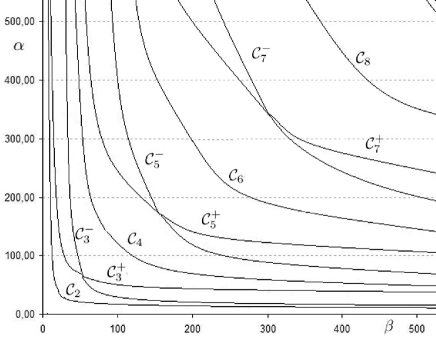
Figure 1. The Fučík spectrum for $m(x)=1+(x+1)^{-1}$ and $n(x)=1+cos^{2}(2x)$.

In Table 1 we compute $\lambda_{4,t}^{+}$ and $t\lambda_{4,t}^{+}$ for different values of $t$ taking $\varepsilon=0.0001$. For $t\to 0$ and $t\to\infty$ we can compare with the eigenvalues $\mu_{2}(m)=23.44031$, $\mu_{2}(n)=29.08$.

Table 1. Eigenvalues $\alpha=\lambda_{4,t}^{+}$ and $\beta=t\lambda_{4,t}^{+}$ for different values of $t$.

t	$\alpha$	$\beta$
$10^{5}\qquad$	23,577	2357747,078
$10^{4}\qquad$	23,939	239291,613
$10^{3}\qquad$	25,110	25110,064
$10^{2}\qquad$	28,994	2899,356
$10\qquad$	43,172	431,716
$1\qquad$	106,483	106,483
$10^{-1}\qquad$	486.812	48,649
$10^{-2}\qquad$	3476.799	34,768
$10^{-3}\qquad$	30800.052	30,800
$10^{-4}\qquad$	295937.669	29,594
$10^{-5}\qquad$	2921329.105	29,213

In Table 2, for a fixed line with $t=30$, we compute the value of $\lambda_{k,t}^{+}$ for several values of $k$ by using the algorithm (21) and we compare the obtained values with the asymptotic values obtained in (20).

Table 2. Higher eigenvalues in a fixed line with $t=30$.

$k$	$\lambda_{k,t}^{+}$	$\lambda_{k,t}^{+}$	Relative error
	(from (20))	(from (21))
10	211,144	212,299	0,005
50	5285,967	5300,702	0,004
100	21145,257	21132,488	0,0006
200	84503,308	84529,952	0,0003
500	528618,283	528312,203	0,0006
1000	2111447,975	2113248,815	0,0008

Finally, for a fixed value of $k=28$, we compare in Table 3 for $\alpha$ the numerical approximation given by (21) and the asymptotic given by (20) varying $t$.

Table 3. Values of $\lambda_{28,t}^{+}$ for different values of $t$.

$t$	$\lambda_{28,t}^{+}$	$\lambda_{28,t}^{+}$	Relative error
	(from (21))	(from (20))
0,1	23202,100	23294,798	0,0039
0,5	7550,103	7588,970	0,0051
1	5094,391	5124,467	0,0058
5	2565,027	2577,485	0,0048
10	2090,991	2099,903	0,0042
1000	1226,496	1231,067	0,0037
100000	1152,512	1156,209	0,0031

References

- [1] M. Alif, Sur le Spectre de Fučík du -Laplacien avec des Poids Indefinis, C. R. Math. Acad. Sci. Paris 334 (2002) 1061–1066.
- [2] M. Alif, J.-P. Gossez, On the Fučík Spectrum with Indefinite Weights, Dif. Int. Eq. 14 (2001) 1511–1530.
- [3] B. M. Brown, W. Reichel, Computing eigenvalues and Fučík spectrum of the radially symmetric -Laplacian, Journal of Computational and Applied Mathematics 148 (2002) 183–211.
- [4] W. Chen, J. Chu, P. Yan, M. Zhang, On the Fučík spectrum of the scalar -Laplacian with indefinite integrable weights, Boundary Value Problems 2014:10 doi:10.1186/1687-2770-2014-10.
- [5] R. Courant, D. Hilbert, Methods of mathematical physics. Vol. I (Interscience Publishers, Inc., New York, N.Y. 1953).
- [6] M. Cuesta, D. de Figueiredo, J.-P. Gossez, The beginning of the Fučik spectrum for the -Laplacian, J. Differential Equations 159 (1999) 212–238.
- [7] E. N. Dancer, On the Dirichlet problem for weakly non-linear elliptic partial differential equations, Proc. Roy. Soc. Edinburgh Sect. A 76 (1976/77) 283–300.
- [8] O. Došlý & P. Řehák, Half-linear differential equations, North-Holland Mathematics Studies, Vol. 202 (Elsevier, 2005).
- [9] J. Fleckinger, M. Lapidus, Remainder estimates for the asymptotics of elliptic eigenvalue problems with indefinite weights, Arch. Rat. Mech. Anal. 98 (1987) 329–356.
- [10] S. Fučík, Boundary value problems with jumping nonlinearities, Časopis Pěst. Mat. 101 (1976) 69–87.
- [11] F. Genoud, P. Rynne, Half eigenvalues and the Fučík spectrum of multi-point, boundary value problems, Journal of Differential Equations 252 (2012) 5076–5095
- [12] J. P. Pinasco, Lower bounds of Fučík eigenvalues of the weighted one-dimensional -Laplacian, Rend. Istit. Mat. Univ. Trieste 36 (2004) 49–64.
- [13] J. P. Pinasco, Lyapunov-type Inequalities with applications to eigenvalue problems (Springer, 2013).
- [14] B. P. Rynne, The Fučík spectrum of general Sturm-Liouville problems, J. Differential Equations 161 (2000) 87–109.