Quantum Statistical Mechanics as an Exact Classical Expansion with Results for Lennard-Jones Helium

Abstract

The quantum states representing classical phase space are given, and these are used to formulate quantum statistical mechanics as a formally exact double perturbation expansion about classical statistical mechanics. One series of quantum contributions arises from the non-commutativity of the position and momentum operators. Although the formulation of the quantum states differs, the present results for separate averages of position operators and of momentum operators agree with Wigner (1932) and Kirkwood (1933). The second series arises from wave function symmetrization, and is given in terms of $l$-particle permutation loops in an infinite order re-summation. The series gives analytically the known exact result for the quantum ideal gas to all orders. The leading correction corrects a correction given by Kirkwood.

The first four quantum corrections to the grand potential are calculated for a Lennard-Jones fluid using the hypernetted chain closure. For helium on liquid branch isotherms, the corrections range from several times to 1% of the total classical pressure, with the effects of non-commutativity being significantly larger in magnitude than those of wave function symmetrization. All corrections are found to be negligible for argon at the densities and temperatures studied. The calculations are computationally trivial as the method avoids having to compute eigenfunctions, eigenvalues, and numerical symmetrization.

I Introduction

Quantum mechanics is fine in theory. But for applications to real-world condensed matter systems, quantum mechanics has proven computationally intractable. The two main impediments are the need to obtain the eigenvalues and eigenfunctions of the system, and the need to symmetrize the wave function. The scaling of both problems with the size of the system is prohibitive.

Faced with these challenges, workers have had two choices. They could choose to focus on a small system and hope to develop techniques to solve it exactly up to a certain level, or else they could look to use approximate approaches on larger systems. As an example of the former, Hernando and VinìčekHernando11 found the first 50 eigenfunctions for five Lennard-Jones particles using a non-uniform discretization of space and time. The algorithm is said to be considerably more efficient than the ${\cal O}(e^{N})$ scaling of standard finite difference methods. Nevertheless the method requires diagonalization of an $M\times M$ sparse matrix, with $M\approx 10^{5}$ for five particles in one dimension, and apparently scaling as ${\cal O}(N^{3})$. This is prior to wave function symmetrization. As an example of an approximate approach, Georgescu and MandelshtamGeorgescu11 approximated the wave functions with unsymmetrised Gaussian wave packets in a variational method and with them studied the ground state of Lennard-Jones clusters of up to 6,500 atoms. This work estimated that the scaling with system size was reduced from ${\cal O}(N^{3})$ to ${\cal O}(N^{2})$. Again this is without wave function symmetrization. The reader is referred to either article for a comprehensive review of the state of the art in computational methods.Hernando11 ; Georgescu11

In contrast, the exact numerical simulation of classical systems is almost trivial, with $10^{3}$–$10^{4}$ particles being routine, and with the computational burden scaling linearly with system size (if a potential cut-off and neighbor tables are used).Allen87 Monte Carlo simulations in particular account exactly for interactions with thermodynamic reservoirs, as do molecular dynamic approaches that include a stochastic thermostat. NETDSM There have been a number of semi-classical approaches to quantum systems that invoke various forms for the wave functions or density matrix (see, for example, Ch. 10 of Ref. Allen87, ), with mixed results.

These observations suggest that it would probably be most efficient to avoid the wave function or density matrix altogether, if this were at all possible, and to instead treat quantum systems as some sort of perturbation expansion of classical systems.

To this end there have been attempts to formulate quantum mechanics in terms of a classical phase space representation of quantum states, with most attention paid to the quasi-probability distribution first introduced by Wigner, and shortly later modified by Kirkwood. Wigner32 ; Kirkwood33 ; Groenewold46 ; Moyal49 ; Zachos05 The Wigner phase space quasi-probability distribution has found applications in quantum optics Barnett03 ; Gerry05 ; Najarbashi16 ; Park16 and quantum information theory.Braunstein05 ; Weedbrook12 The Wigner and Kirkwood quasi-probability functions are similar but not identical, which can be said of all the phase space quasi-probability functions that have been proposed.Praxmeyer02 ; Dishlieva08

The phase space quasi-probability distribution given by WignerWigner32 neglected wave function symmetrization, whereas that given by KirkwoodKirkwood33 accounted for the leading order correction (ie. the single transposition of a pair of particles). The sometimes dramatic effects that are observed to arise from particle statistics in some systems suggests that the approximation of Wigner, Kirkwood, and followers may not always capture the most important quantum corrections to the classical.

The present paper also seeks the quantum states that correspond to classical phase space, with the aim of developing a perturbation expansion for quantum statistical mechanics that has classical statistical mechanics as the leading order term. The twin motivations are the relative computational simplicity of classical systems, and also the observation that quantum effects are but a small perturbation for most terrestrial condensed matter systems.

The reasons for focussing on quantum statistical mechanics rather than on quantum mechanics are both practical (real world problems are thermodynamic in nature, and at the molecular level large systems are most efficiently treated statistically), and, more importantly, conceptual. Quantum statistical mechanics applies to open quantum systems, and in these the wave function has collapsed into mixed quantum states with no interference. Zurek03 ; Davies76 ; Breuer02 ; Weiss08 ; Zeh01 ; QSM1 ; QSM This marks the distinction between the quantum and the classical. With quantum statistical mechanics formulated as the sum over states of the Maxwell-Boltzmann operator,Neumann27 one sees the beginning of the connection with classical statistical mechanics, which is essentially the integral over classical phase space of Maxwell-Boltzmann probability.

So the end-point point is clear —a theory of condensed matter with classical statistical mechanics as the leading order term. As also is the starting point —quantum statistical mechanics. This paper maps the route between the two.

In §II.1 the grand partition function is formally written as the sum over unique states by invoking an overlap factor for double counting due to wave function symmetrization. In §II.2 the basis wave functions that lead to classical phase space are given, and in §II.3 the grand partition function is formulated in terms of them. In §II.4 the Maxwell-Boltzmann operator is recast as a function suitable for expansion in powers of Planck’s constant, which accounts for the non-commutativity of the position and momentum operators, and in §II.5 this is incorporated into the grand partition function as a weight for phase space. In §II.6 the permutations that comprise the overlap factor for wave function symmetrization are written as a sum over distinct permutation loops, which allows the grand partition function to be resummed and the grand potential to be written as a sum of classical equilibrium averages over phase space of the loops. In §II.7 the statistical average of a quantum operator is expressed in the same formalism. In §III the formalism is compared with known results, and in §IV numerical results for the quantum corrections in liquid helium are given.

II Formal Analysis

II.1 Symmetrization, Overlap, and the Grand Partition Function

The grand partition function for a quantum system is Neumann27 ; Messiah61 ; Merzbacher70 ; QSM1 ; QSM ; Attard16

$$\Xi = \mbox{TR }z^{N}e^{-\beta\hat{\cal H}}$$ (2.1)

$$= \sum_{N=0}^{\infty}z^{N}\sum_{\bf m}\!^{\prime}e^{-\beta{\cal H}_{\bf m}}$$

$$= \sum_{N=0}^{\infty}\frac{z^{N}}{N!}\sum_{\bf m}\chi_{\bf m}e^{-\beta{\cal H}_{\bf m}}.$$

Here $N$ is the number of particles, the fugacity is $z\equiv e^{\beta\mu}$, where $\mu$ is the chemical potential, $\beta=1/k_{\mathrm{B}}T$ is sometimes called the inverse temperature, with $k_{\mathrm{B}}$ being Boltzmann’s constant and $T$ the temperature, and $\hat{\cal H}$ is the Hamiltonian or energy operator. The first equality is the conventional expression, Neumann27 ; Messiah61 ; Merzbacher70 ; QSM1 ; QSM and perhaps also the second;Messiah61 ; Attard16 the final equality, not so much.Attard16

In the second equality the prime on the summation indicates that the sum is over distinct entropy states.Messiah61 ; Attard16 Some authors, specifically Kirkwood,Kirkwood33 and some text book writers, specifically Pathria,Pathria72 neglect this point. Since the entropy operator is proportional to the energy operator, $\hat{S}_{\mathrm{r}}=-\hat{\cal H}/T$, entropy states are the same as energy states, entropy eigenvalues are proportional to energy eigenvalues, $S_{\mathrm{r},{\bf m}}=-{\cal H}_{\bf m}/T$, and the entropy eigenfunctions $\phi_{\bf m}$ are also energy eigenfunctions. (The grand partition function is not restricted to entropy states, but it is these that originally give rise to the form, and it is these that are shortly used to introduce the expectation value.)

In the third equality the sum over all entropy states has been invoked, with the factor $\chi_{\bf m}/N!$, which is explained next, properly accounting for the fact that some states are counted multiple times. Attard16

In quantum mechanics, under particle interchange the wave function is fully symmetric for identical bosons and fully anti-symmetric for identical fermions. Hence the basis wave functions must be symmetrized from the more general basis wave functions by writing Messiah61 ; Merzbacher70 ; Attard16

$$\phi_{{\bf m}}^{\mathrm{S/A}}({\bf r})\equiv\frac{1}{\sqrt{N!\chi^{\pm}(\phi_{\bf m})}}\sum_{\hat{\mathrm{P}}}(\pm 1)^{p}\,\phi_{{\bf m}}(\hat{\mathrm{P}}{\bf r}).$$ (2.2)

Here ${\bf r}$ are the particle coordinates, which is to say that the position representation is invoked here and below. Below $\phi_{{\bf m}}$ will be taken to be an entropy (equivalently, energy) eigenfunction, although this symmetrization equation in fact holds for any wave function. The superscript S signifies symmetric, and it applies for bosons using $(+1)^{p}=1$ on the right hand side. The superscript A signifies anti-symmetric, and it applies for fermions using $(-1)^{p}$ on the right hand side. Here $\hat{\mathrm{P}}$ is the permutation operator, and $p$ is its parity (ie. the number of pair transpositions that comprise the permutation). One can equivalently permute instead the state label ${\bf m}$.

The prefactor including $\chi_{\bf m}$ ensures the correct normalization,

$$\langle\phi^{\mathrm{S/A}}_{\bf m^{\prime}}\,|\,\phi^{\mathrm{S/A}}_{\bf m}\rangle=\delta_{{\bf m}^{\prime},{\bf m}},$$ (2.3)

where the Kronecker-$\delta$ function appears. Inserting in this the expression for the symmetrized wave function and rearranging gives the overlap factor as

$$\chi^{\pm}(\phi_{\bf m}) = \frac{1}{N!}\sum_{\hat{\mathrm{P}},\hat{\mathrm{P}}^{\prime}}(\pm 1)^{p+p^{\prime}}\langle\phi_{{\bf m}}(\hat{\mathrm{P}}{\bf r})|\phi_{{\bf m}}(\hat{\mathrm{P}}^{\prime}{\bf r})\rangle$$ (2.4)

$$= \sum_{\hat{\mathrm{P}}}(\pm 1)^{p}\langle\phi_{{\bf m}}(\hat{\mathrm{P}}{\bf r})|\phi_{{\bf m}}({\bf r})\rangle$$

$$= \sum_{\hat{\mathrm{P}}}(\pm 1)^{p}\int\mathrm{d}{\bf r}\;\phi_{{\bf m}}(\hat{\mathrm{P}}{\bf r})^{*}\phi_{{\bf m}}({\bf r}).$$

This shows that in each case the overlap factor depends upon the chosen basis wave functions. This quantity is called the overlap factor because it tells how much symmetrization counts the same microstate multiple times. The formula for the overlap factor, Eq. (2.4), holds for multi-particle states, as well as for when the entropy microstate consists of one-particle states. For a detailed discussion see Ref. Attard16, .

In general for identical particles the Hamiltonian operator is unchanged by a permutation of the particles,

$$\hat{\cal H}({\bf r})=\hat{\cal H}(\hat{\mathrm{P}}{\bf r}).$$ (2.5)

In this work the Hamiltonian operator is taken to be

$$\hat{\cal H}({\bf r})=U({\bf r})-\frac{\hbar^{2}}{2m}\nabla^{2},$$ (2.6)

where $U({\bf r})$ is the potential energy, $\hbar$ is Planck’s constant divided by $2\pi$, and $m$ is the particle mass.

Let the basis wave functions $\phi_{\bf m}$ be entropy eigenfunctions. Hence they are also energy eigenfunctions,

$$\hat{\cal H}({\bf r})\phi_{\bf m}({\bf r})={\cal H}_{\bf m}\phi_{\bf m}({\bf r}).$$ (2.7)

Obviously the symmetrized basis wave functions are also eigenfunctions of the entropy operator with unchanged eigenvalues.

The grand partition function given above can be recast explicitly in terms of the entropy eigenfunctions,

$$\Xi^{\pm} = \sum_{N}\frac{z^{N}}{N!}\sum_{\bf m}\chi^{\pm}(\phi_{\bf m})e^{-\beta{\cal H}_{\bf m}}$$ (2.8)

$$= \sum_{N}\frac{z^{N}}{N!}\sum_{\bf m}\sum_{\hat{\mathrm{P}}}(\pm 1)^{p}\langle\phi_{\hat{\mathrm{P}}{\bf m}}|\phi_{{\bf m}}\rangle e^{-\beta{\cal H}_{\bf m}}$$

$$= \sum_{N}\frac{z^{N}}{N!}\sum_{\bf m}\sum_{\hat{\mathrm{P}}}(\pm 1)^{p}\langle\phi_{\hat{\mathrm{P}}{\bf m}}|e^{-\beta\hat{\cal H}}|\phi_{\bf m}\rangle.$$

This formulation of the grand partition function as a (permuted) expectation value is a small but significant modification of the original.Attard16 Although derived for entropy basis functions, the expectation value holds for any set of basis functions, which has the advantage that one does not have to find the entropy eigenfunctions. This formulation as an expectation value provides the starting point for the present paper.

II.2 Basis Functions

It is an important conceptual point, in this section and in the rest of the paper, that there is a distinction between the coordinate positions, ${\bf r}$, and the configurations positions ${\bf q}$. The coordinate positions appear as the argument of the wave function and operators in the position representation. The coordinate positions appear in classical phase space. Essentially, the conceptual distinction between the two is that the coordinate positions ${\bf r}$ are a representation, and the configuration positions ${\bf q}$ are a quantum state.

The predecessors of the present author, specifically WignerWigner32 and Kirkwood,Kirkwood33 treat these as the same thing.fn1 The present paper keeps them distinct. To be sure, as is detailed below, a zero-width limit is invoked in which certain wave functions become Dirac-$\delta$ functions, $\delta({\bf r}-{\bf q})$, and in this limit the two quantities become equal to each other. But the point to emphasize is that this limit is invoked after certain mathematical manipulations. It is essential to keep in mind the passage to this limit in order to achieve the final results.

II.2.1 Wave Packets

In Ref. Attard16, the problem of quantum statistical mechanics was approached by using minimum uncertainty wave packets as the basis for the basis functions. These are

$$\zeta_{{\bf q}{\bf p}}({\bf r})=\frac{1}{(2\pi\xi^{2})^{3N/4}}e^{-{\varepsilon}_{{\bf q}}({\bf r})^{2}/4\xi^{2}}e^{-{\bf p}\cdot{\bm{\varepsilon}}_{{\bf q}}({\bf r})/i\hbar},$$ (2.9)

where ${\bm{\varepsilon}}_{{\bf q}}({\bf r})\equiv{\bf r}-{\bf q}$. For $N$ particles in three dimensions, the vectors are 3N-dimensional, with ${\bf r}$ being the coordinate positions, ${\bf q}$ being the configuration positions, and ${\bf p}$ being the configuration momenta.

The motivation for using these as the starting point of the analysis was that they are approximately entropy (energy) eigenfunctions,

$$\hat{\cal H}({\bf r})\,\zeta_{{\bf q}{\bf p}}({\bf r})$$ (2.10)

$$= \left\{U({\bf r})+\frac{1}{2m}{\bf p}\cdot{\bf p}+\frac{3N\hbar^{2}}{4m\xi^{2}}\right.$$

$$\left.\mbox{ }-\frac{\hbar^{2}}{8m\xi^{4}}{\bm{\varepsilon}}_{{\bf q}}({\bf r})\cdot{\bm{\varepsilon}}_{{\bf q}}({\bf r})-\frac{\hbar^{2}}{2mi\hbar\xi^{2}}{\bm{\varepsilon}}_{{\bf q}}({\bf r})\cdot{\bf p}\right\}\zeta_{{\bf q}{\bf p}}({\bf r})$$

$$\approx \left\{{\cal H}({\bf\Gamma})+\frac{3N\hbar^{2}}{4m\xi^{2}}\right\}\zeta_{{\bf q}{\bf p}}({\bf r}),$$

where a point in classical phase space is ${\bf\Gamma}\equiv\{{\bf q},{\bf p}\}$. The second equality assumes that the wave packet is sharply peaked so that terms involving powers of ${\bm{\varepsilon}}_{{\bf q}}({\bf r})$ can be neglected. This includes the terms in the expansion of $U({\bf r})=U({\bf q})+{\bm{\varepsilon}}_{{\bf q}}({\bf r})\cdot{\bf U}^{\prime}({\bf q})+\ldots$. The classical Hamiltonian is

$${\cal H}({\bf\Gamma})=\frac{1}{2m}{\bf p}\cdot{\bf p}+U({\bf q}).$$ (2.11)

Since one expects that any expansion of quantum statistical mechanics will have classical statistical mechanics as the leading term, this provided two further motivations for using wave packets, namely that the classical Hamiltonian is the approximate eigenvalue, and points in classical phase space are the index of the wave packets.

Despite these advantages wave packets have several disadvantages. The first is that they are approximate, not exact, entropy eigenfunctions. The algebra required to systematically modify them so as to reduce the error in the approximation rapidly proliferates, as does the computational complexity.Attard16 The second is that they do not form an exact basis set because they overlap for finite wave packet widths $\xi$ and they are therefore non-orthogonal. With the wisdom of hindsight, the latter problem appears prohibitive.

Nevertheless, the original motivation —that minimum uncertainty wave packets are close to entropy eigenfunctions, and that their indeces are points in classical phase space— remain compelling. It turns out to be exceedingly fruitful to instead consider two closely related basis sets.

II.2.2 Plane Waves

One half of the wave packets given above are plane waves. Plane waves localize the momenta of the particles. They are in fact kinetic energy eigenfunctions. These motivate considering plane waves as a basis set,

$$\zeta_{\bf p}({\bf r}) = \frac{1}{V^{N/2}}e^{-{\bf p}\cdot{\bf r}/i\hbar}$$ (2.12)

$$= \prod_{j=1}^{N}\frac{e^{-{\bf p}_{j}\cdot{\bf r}_{j}/i\hbar}}{V^{1/2}},$$

with the configuration momentum being ${\bf p}=2\pi\hbar{\bf n}/V^{1/3}$, $n=0,\pm 1,\pm 2,\ldots$, and $V$ the volume. The quantization arises from imposing periodic boundary conditions. From this the width of a momentum state is evidently

$$\Delta_{p}=2\pi\hbar/V^{1/3}.$$ (2.13)

This is used below in taking the continuum limit, after which quantization of the momentum index becomes irrelevant.

Plane waves are orthonormal,

$$\langle\zeta_{{\bf p}^{\prime}}|\zeta_{\bf p}\rangle = \frac{1}{V^{N}}\int\mathrm{d}{\bf r}\;e^{-{\bf r}\cdot({\bf p}-{\bf p}^{\prime})/i\hbar}$$ (2.14)

$$= \delta_{{\bf p}^{\prime},{\bf p}},$$

as follows from the boundary conditions. They also form a complete set,

$$\sum_{\bf p}\zeta_{\bf p}({\bf r}^{\prime})^{*}\zeta_{\bf p}({\bf r}) = \frac{V^{-N}}{(2\pi\hbar V^{-1/3})^{3N}}\int\mathrm{d}{\bf p}\;e^{-{\bf p}\cdot({\bf r}-{\bf r}^{\prime})/i\hbar}$$ (2.15)

$$= \delta({\bf r}-{\bf r}^{\prime}),$$

since $\int\mathrm{d}x\,e^{ikx}=2\pi\delta(k)$. In bra-ket notation completeness is written $\sum_{\bf p}|\zeta_{\bf p}\rangle\,\langle\zeta_{\bf p}|=\hat{\mathrm{I}}$.

II.2.3 Gaussians

The other half of wave packets are Gaussians, which localize the positions of the particles. Here they are taken to be

$$\zeta_{\bf q}({\bf r}) = \frac{e^{-({\bf r}-{\bf q})^{2}/4\xi^{2}}}{(2\pi\xi^{2})^{3N/4}}$$ (2.16)

$$= \prod_{j=1}^{N}\frac{e^{-({\bf r}_{j}-{\bf q}_{j})^{2}/4\xi^{2}}}{(2\pi\xi^{2})^{3/4}}.$$

(Using $4\xi^{2}$ rather than say $2\xi^{2}$ in the exponent is an evolutionary accident; its parent is the minimal uncertainty wave packet. There is nothing significant in it and it in no way affects the following results.)

The overlap or orthonormality of such Gaussians is

$$\langle\zeta_{\bf q}|\zeta_{{\bf q}^{\prime}}\rangle = \frac{1}{(2\pi\xi^{2})^{3N/2}}\int\mathrm{d}{\bf r}\;e^{-({\bf r}-{\bf q})^{2}/4\xi^{2}}e^{-({\bf r}-{\bf q}^{\prime})^{2}/4\xi^{2}}$$ (2.17)

$$= e^{-({\bf q}-{\bf q}^{\prime})^{2}/8\xi^{2}}$$

$$\equiv \delta_{\xi}({\bf q},{\bf q}^{\prime}).$$

This is a soft Kronecker-$\delta$ that becomes an exact Kronecker-$\delta$ in the limit $\xi\rightarrow 0$.

The completeness of the set of Gaussians is manifest as

$$\sum_{\bf q}|\zeta_{\bf q}({\bf r}^{\prime})\rangle\,\langle\zeta_{\bf q}({\bf r})|$$ (2.18)

$$= \frac{1}{\Delta_{q}^{3N}}\int\mathrm{d}{\bf q}\;\zeta_{{\bf q}}({\bf r})^{*}\,\zeta_{{\bf q}}({\bf r}^{\prime})$$

$$= \frac{(2\pi\xi^{2})^{-3N/2}}{\Delta_{q}^{3N}}\int\mathrm{d}{\bf q}\;e^{-({\bf r}-{\bf q})^{2}/4\xi^{2}}e^{-({\bf r}^{\prime}-{\bf q})^{2}/4\xi^{2}}$$

$$= \frac{1}{\Delta_{q}^{3N}}e^{-({\bf r}^{\prime}-{\bf r})^{2}/8\xi^{2}}.$$

Normalization (ie. demanding that this integrate to unity) fixes the spacing of the configuration position states as

$$\Delta_{q}=\sqrt{8\pi\xi^{2}}.$$ (2.19)

The completeness now is

$$\sum_{\bf q}|\zeta_{\bf q}({\bf r}^{\prime})\rangle\,\langle\zeta_{\bf q}({\bf r})| = \frac{e^{-({\bf r}^{\prime}-{\bf r})^{2}/8\xi^{2}}}{(8\pi\xi^{2})^{3N/2}}$$ (2.20)

$$\equiv \delta_{\xi}({\bf r}^{\prime}-{\bf r}).$$

This is a soft Dirac-$\delta$ function that is normalized and that becomes an exact Dirac-$\delta$ function in the limit $\xi\rightarrow 0$. Hence

$$\lim_{\xi\rightarrow 0}\sum_{\bf q}|\zeta_{\bf q}\rangle\,\langle\zeta_{\bf q}|=\hat{\mathrm{I}}.$$ (2.21)

One concludes that Gaussians form a basis set that is orthonormal and complete in the limit that the width of the Gaussian goes to zero. The fact that this Gaussian becomes a generalized function in the zero width limit is no cause for concern. The real test of the theory is whether or not its final formulation is finite and well-behaved in the zero width limit.

A Gaussian can be expanded in terms of plane waves (and vice versa). One has

$$\zeta_{\bf q}({\bf r})=\sum_{\bf p}g_{\bf p}({\bf q})\zeta_{\bf p}({\bf r}),$$ (2.22)

with the coefficients being

$$g_{\bf p}({\bf q}) = \langle\zeta_{\bf p}|\zeta_{\bf q}\rangle$$ (2.23)

$$= \frac{V^{-N/2}}{(2\pi\xi^{2})^{3N/4}}\int\mathrm{d}{\bf r}\,e^{-({\bf r}-{\bf q})^{2}/4\xi^{2}}e^{{\bf p}\cdot{\bf r}/i\hbar}$$

$$= \frac{V^{-N/2}}{(2\pi\xi^{2})^{3N/4}}\int\mathrm{d}{\bf r}\,e^{-({\bf r}-{\bf q}-2\xi^{2}{\bf p}/i\hbar)^{2}/4\xi^{2}}$$

$$\times\mbox{ }e^{{\bf q}\cdot{\bf p}/i\hbar}e^{-\xi^{2}p^{2}/\hbar^{2}}$$

$$= \frac{(8\pi\xi^{2})^{3N/4}}{V^{N/2}}e^{-\xi^{2}p^{2}/\hbar^{2}}e^{{\bf q}\cdot{\bf p}/i\hbar}.$$

It will sometimes prove useful to write this as the product of individual single particle factors

$$g_{\bf p}({\bf q}) = \prod_{j=1}^{N}\frac{(8\pi\xi^{2})^{3/4}}{V^{1/2}}e^{-\xi^{2}p_{j}^{2}/\hbar^{2}}e^{{\bf q}_{j}\cdot{\bf p}_{j}/i\hbar}$$ (2.24)

$$\equiv \prod_{j=1}^{N}g_{{\bf p}_{j}}({\bf q}_{j}).$$

The limit ${\xi\rightarrow 0}$ will be invoked during the analysis, as expedient.

Finally, it seems straightforward to include spin in the theory by multiplying the various basis functions by the product of single particle spin functions. This has not been done here in order to keep the theory as simple as possible and to keep the focus on the main aim of a phase space formulation of quantum statistical mechanics.

II.3 Phase Space Representation of Quantum States

The fact that plane waves form an orthonormal, complete basis set means that the grand partition function, Eq. (2.8), may be written as a sum over them. This could simply be written down directly, since the trace operation is universal and it can be expressed as the sum over the set of any basis states. However it is worthwhile to illustrate the use of the completeness property, and in full the derivation is

$$\Xi^{\pm} = \sum_{N}\frac{z^{N}}{N!}\sum_{\bf m}\sum_{\hat{\mathrm{P}}}(\pm 1)^{p}\langle\phi_{\hat{\mathrm{P}}{\bf m}}|e^{-\beta\hat{\cal H}}|\phi_{\bf m}\rangle$$ (2.25)

$$= \sum_{N}\frac{z^{N}}{N!}\sum_{\bf m}\sum_{{\bf p},{\bf p}^{\prime}}\sum_{\hat{\mathrm{P}}}(\pm 1)^{p}$$

$$\mbox{ }\times\langle\phi_{\hat{\mathrm{P}}{\bf m}}|\zeta_{\bf p}\rangle\,\langle\zeta_{\bf p}|e^{-\beta\hat{\cal H}}|\zeta_{{\bf p}^{\prime}}\rangle\,\langle\zeta_{{\bf p}^{\prime}}|\phi_{\bf m}\rangle$$

$$= \sum_{N}\frac{z^{N}}{N!}\sum_{{\bf p},{\bf p}^{\prime}}\sum_{\hat{\mathrm{P}}}(\pm 1)^{p}\langle\zeta_{\bf p}|e^{-\beta\hat{\cal H}}|\zeta_{{\bf p}^{\prime}}\rangle\,\langle\zeta_{{\bf p}^{\prime}}|\zeta_{\hat{\mathrm{P}}{\bf p}}\rangle$$

$$= \sum_{N}\frac{z^{N}}{N!}\sum_{{\bf p}}\sum_{\hat{\mathrm{P}}}(\pm 1)^{p}\langle\zeta_{\bf p}|e^{-\beta\hat{\cal H}}|\zeta_{\hat{\mathrm{P}}{\bf p}}\rangle.$$

In the same way the completeness of the Gaussian basis functions, Eq. (2.20), and their expansion in terms of plane waves, Eq. (2.22), enable this to be re-written

$$\Xi^{\pm} = \sum_{N}\frac{z^{N}}{N!}\sum_{\bf p}\sum_{\hat{\mathrm{P}}}(\pm 1)^{p}\langle\zeta_{{\bf p}}|e^{-\beta\hat{\cal H}}|\zeta_{\hat{\mathrm{P}}{\bf p}}\rangle$$ (2.26)

$$= \sum_{N}\frac{z^{N}}{N!}\sum_{{\bf q}}\sum_{\bf p}\sum_{\hat{\mathrm{P}}}(\pm 1)^{p}\langle\zeta_{\bf p}|\zeta_{{\bf q}}\rangle\,\langle\zeta_{{\bf q}}|e^{-\beta\hat{\cal H}}|\zeta_{\hat{\mathrm{P}}{\bf p}}\rangle$$

$$= \sum_{N}\frac{z^{N}}{N!}\sum_{{\bf q},{\bf p}}g_{\bf p}({\bf q})\sum_{\hat{\mathrm{P}}}(\pm 1)^{p}\langle\zeta_{{\bf q}}|e^{-\beta\hat{\cal H}}|\zeta_{\hat{\mathrm{P}}{\bf p}}\rangle$$

$$\equiv \sum_{N}\frac{z^{N}}{N!}\sum_{{\bf q},{\bf p}}g_{\bf p}({\bf q})\chi^{\pm}_{\cal H}(\zeta_{\bf q},\zeta_{\bf p}).$$

It is emphasized that this formulation is formally exact in the limit $\xi\rightarrow 0$.

The immediate and obvious merit of formulating the problem in terms of this asymmetric expectation value is that the sum over states has become a sum over points in classical phase space. The continuum limit is

$$\sum_{{\bf q},{\bf p}}\Rightarrow\frac{1}{(\Delta_{p}\Delta_{q})^{3N}}\int\mathrm{d}{\bf\Gamma}.$$ (2.27)

The volume elements are those derived above for plane waves, $\Delta_{p}=2\pi\hbar/V^{1/3}$, and for Gaussians, $\Delta_{q}=\sqrt{8\pi\xi^{2}}$.

One sees from this that the combination of plane waves and Gaussian basis sets in an asymmetric expectation value provides a way of representing classical phase space. The plane waves localize the momenta, and the Gaussians localize the positions. This way of representing phase space is distinctly different to the way advocated by Wigner,Wigner32 Kirkwood,Kirkwood33 and followers. Groenewold46 ; Moyal49 ; Barnett03 ; Gerry05 ; Zachos05 ; Praxmeyer02 ; Dishlieva08

The final equality for the grand partition function defines the weighted overlap factor,

$$\chi^{\pm}_{\cal H}(\zeta_{\bf q},\zeta_{\bf p}) \equiv \sum_{\hat{\mathrm{P}}}(\pm 1)^{p}\langle\zeta_{\hat{\mathrm{P}}{\bf q}}|e^{-\beta\hat{\cal H}}|\zeta_{{\bf p}}\rangle$$

$$= \sum_{\hat{\mathrm{P}}}(\pm 1)^{p}\int\mathrm{d}{\bf r}\;\zeta_{{\bf q}}(\hat{\mathrm{P}}{\bf r})^{*}e^{-\beta\hat{\cal H}({\bf r})}\zeta_{{\bf p}}({\bf r}).$$

Because one is summing over all permutations and states, it makes no difference to which wave function index or coordinate argument the permutator is applied.

It is worth mentioning that here the Maxwell-Boltzmann operator is explicitly shown as acting on the plane wave basis function. One could have formulated the problem with the opposite asymmetry so that it acted on the Gaussian basis function (or else just use its properties as a Hermitian operator). In view of the results obtained in the following sub-section, the present formulation is the simplest.

II.4 Expansion of the Maxwell-Boltzmann Operator

WignerWigner32 , in developing his pseudo-probability distribution for phase space as a type of Fourier transform of a mixture of wave functions, gave a useful result for the transformation of the Maxwell-Boltzmann position coordinate matrix. That result may be exploited here for the action of the Maxwell-Boltzmann operator on the plane wave basis functions.

In general one has for the operator equation

$$e^{{\bf p}\cdot{\bf r}/i\hbar}f(\hat{O})e^{-{\bf p}\cdot{\bf r}/i\hbar}=f(\hat{\tilde{O}}),\;\;\hat{\tilde{O}}\equiv e^{{\bf p}\cdot{\bf r}/i\hbar}\hat{O}e^{-{\bf p}\cdot{\bf r}/i\hbar},$$ (2.29)

as can be confirmed by writing $f(x)$ as a power series. Hence the action of the Maxwell-Boltzmann operator on a plane wave basis function can be written as

$$e^{-\beta\hat{{\cal H}}}\zeta_{\bf p}({\bf r}) = \zeta_{\bf p}({\bf r})e^{-\beta\hat{\tilde{\cal H}}}1$$ (2.30)

$$\equiv \zeta_{\bf p}({\bf r})e^{-\beta{\cal H}({\bf r},{\bf p})}W({\bf r},{\bf p}).$$

The 1 written explicitly here is a reminder that the operator acts on the constant unit wave function. This arises because the left hand side is a wave function, and one cannot have on the right hand side an operator hanging with nothing to act on. The modified energy operator that is induced by this is

$$\hat{\tilde{\cal H}} \equiv e^{{\bf p}\cdot{\bf r}/i\hbar}\hat{\cal H}e^{-{\bf p}\cdot{\bf r}/i\hbar}$$ (2.31)

$$= e^{{\bf p}\cdot{\bf r}/i\hbar}\left[\frac{-\hbar^{2}}{2m}\nabla^{2}+U({\bf r})\right]e^{-{\bf p}\cdot{\bf r}/i\hbar}$$

$$= \frac{p^{2}}{2m}+U({\bf r})-\frac{i\hbar}{m}{\bf p}\cdot\nabla-\frac{\hbar^{2}}{2m}\nabla^{2}.$$

In the above a phase function $W({\bf r},{\bf p})$ was defined that satisfies

$$e^{-\beta{\hat{\tilde{\cal H}}}}1=e^{-\beta{\cal H}({\bf r},{\bf p})}W({\bf r},{\bf p}).$$ (2.32)

By inspection, $W(\beta=0)=1$. This will provide the basis for an expansion in powers of $\hbar$,

$$W=\sum_{n=0}^{\infty}W_{n}\hbar^{n}.$$ (2.33)

The term $W_{0}=1$ is the classical term, and the terms $W_{n}$, $n\geq 1$ may be called the quantum corrections due to non-commutativity. They arise from the action of the kinetic energy operator on the potential energy and they involve gradients of the potential energy. An alternative formulation of this particular quantum correction is given in appendices A and B.

The temperature derivative of the left hand side is

$$\frac{\partial}{\partial\beta}e^{-\beta{\hat{\tilde{\cal H}}}}1 = -{\hat{\tilde{\cal H}}}e^{-\beta{\hat{\tilde{\cal H}}}}1$$ (2.34)

$$= -{\hat{\tilde{\cal H}}}\left\{e^{-\beta{\cal H}}W\right\},$$

and that of the right hand side is

$$\frac{\partial}{\partial\beta}\left\{e^{-\beta{\cal H}}W\right\} = \left\{\frac{\partial W}{\partial\beta}-{\cal H}\right\}e^{-\beta{\cal H}}W.$$ (2.35)

Equating these and rearranging gives

$$\frac{\partial W}{\partial\beta} = {\cal H}W-e^{\beta{\cal H}}{\hat{\tilde{\cal H}}}\left\{e^{-\beta{\cal H}}W\right\}$$ (2.36)

$$= \frac{i\hbar}{m}e^{\beta U}{\bf p}\cdot\nabla\left\{e^{-\beta U}W\right\}$$

$$\mbox{ }+\frac{\hbar^{2}}{2m}e^{\beta U}\nabla^{2}\left\{e^{-\beta U}W\right\}.$$

Integrating, with $W(\beta=0)=1$,

$$W = 1+\frac{i\hbar}{m}\int_{0}^{\beta}\mathrm{d}\beta^{\prime}\;e^{\beta^{\prime}U}{\bf p}\cdot\nabla\left\{e^{-\beta^{\prime}U}W(\beta^{\prime})\right\}$$

$$\mbox{ }+\frac{\hbar^{2}}{2m}\int_{0}^{\beta}\mathrm{d}\beta^{\prime}\;e^{\beta^{\prime}U}\nabla^{2}\left\{e^{-\beta^{\prime}U}W(\beta^{\prime})\right\}.$$

This is essentially identical to an expression given by Kirkwood for the case of the identity permutation.Kirkwood33 (In the present paper wave function symmetrization is treated differently to Kirkwood.)

Successive substitution gives $W_{0}=1$, the first order correction as

$$W_{1} = \frac{i}{m}\int_{0}^{\beta}\mathrm{d}\beta^{\prime}\;e^{\beta^{\prime}U}{\bf p}\cdot\nabla\left\{e^{-\beta^{\prime}U}W_{0}(\beta^{\prime})\right\}$$ (2.38)

$$= \frac{i}{m}\int_{0}^{\beta}\mathrm{d}\beta^{\prime}\;(-\beta^{\prime}){\bf p}\cdot\nabla U$$

$$= \frac{-i\beta^{2}}{2m}{\bf p}\cdot\nabla U,$$

and the second order correction as

$$W_{2} = \frac{i}{m}\int_{0}^{\beta}\mathrm{d}\beta^{\prime}\;e^{\beta^{\prime}U}{\bf p}\cdot\nabla\left\{e^{-\beta^{\prime}U}W_{1}(\beta^{\prime})\right\}$$ (2.39)

$$\mbox{ }+\frac{1}{2m}\int_{0}^{\beta}\mathrm{d}\beta^{\prime}\;e^{\beta^{\prime}U}\nabla^{2}\left\{e^{-\beta^{\prime}U}W_{0}(\beta^{\prime})\right\}$$

$$= \frac{i}{m}\int_{0}^{\beta}\mathrm{d}\beta^{\prime}\;\left[(-\beta^{\prime})({\bf p}\cdot\nabla U)\times\frac{-i\beta^{\prime 2}}{2m}{\bf p}\cdot\nabla U\right.$$

$$\left.\mbox{ }+\frac{-i\beta^{\prime 2}}{2m}({\bf p}\cdot\nabla)^{2}U\right]$$

$$\mbox{ }+\frac{1}{2m}\int_{0}^{\beta}\mathrm{d}\beta^{\prime}\;\left\{-\beta^{\prime}\nabla^{2}U+\beta^{\prime 2}\nabla U\cdot\nabla U\right\}$$

$$= \frac{-\beta^{4}}{8m^{2}}({\bf p}\cdot\nabla U)^{2}+\frac{\beta^{3}}{6m^{2}}({\bf p}\cdot\nabla)^{2}U$$

$$\mbox{ }-\frac{\beta^{2}}{4m}\nabla^{2}U+\frac{\beta^{3}}{6m}\nabla U\cdot\nabla U.$$

These are essentially the same as Kirkwood’s Eq. (16).Kirkwood33 In general

$$W_{n} = \frac{i}{m}\int_{0}^{\beta}\mathrm{d}\beta^{\prime}\;e^{\beta^{\prime}U}{\bf p}\cdot\nabla\left\{e^{-\beta^{\prime}U}W_{n-1}(\beta^{\prime})\right\}$$

$$\mbox{ }+\frac{1}{2m}\int_{0}^{\beta}\mathrm{d}\beta^{\prime}\;e^{\beta^{\prime}U}\nabla^{2}\left\{e^{-\beta^{\prime}U}W_{n-2}(\beta^{\prime})\right\}.$$

This is essentially the same as Kirkwood’s Eq. (17).Kirkwood33

It is shown below that $W_{1}$ plus $W_{2}$ (and neglecting symmetrization corrections) give a configuration position probability density, §III.2.1, and an average kinetic energy, §III.2.2, that are the same as that given by WignerWigner32 and by Kirkwood.Kirkwood33 It is shown in §III.2.3 that including the first correction for symmetrization and $W_{1}$ essentially agrees with a result given by KirkwoodKirkwood33 (apart from a factor of 2 that arises because Kirkwood does not correct for double counting).

II.5 Overlap Factor

With the above expression that writes the action of the Maxwell-Boltzmann operator on a plane wave basis function as a sum of quantum corrections, Eq. (2.30), the weighted overlap factor, Eq. (II.3), becomes

$$\chi^{\pm}_{\cal H}(\zeta_{\bf q},\zeta_{\bf p})$$ (2.41)

$$\equiv \sum_{\hat{\mathrm{P}}}(\pm 1)^{p}\langle\zeta_{\hat{\mathrm{P}}{\bf q}}|e^{-\beta\hat{\cal H}}|\zeta_{{\bf p}}\rangle$$

$$= \sum_{\hat{\mathrm{P}}}(\pm 1)^{p}\int\mathrm{d}{\bf r}\;\zeta_{\hat{\mathrm{P}}{\bf q}}({\bf r})^{*}e^{-\beta\hat{\cal H}({\bf r})}\zeta_{{\bf p}}({\bf r})$$

$$= \sum_{\hat{\mathrm{P}}}(\pm 1)^{p}\int\mathrm{d}{\bf r}\;\zeta_{\hat{\mathrm{P}}{\bf q}}({\bf r})^{*}\zeta_{{\bf p}}({\bf r})e^{-\beta{\cal H}({\bf r},{\bf p})}W({\bf r},{\bf p})$$

$$= \sum_{\hat{\mathrm{P}}}(\pm 1)^{p}e^{-\beta{\cal H}(\hat{\mathrm{P}}{\bf q},{\bf p})}W(\hat{\mathrm{P}}{\bf q},{\bf p})\int\mathrm{d}{\bf r}\;\zeta_{\hat{\mathrm{P}}{\bf q}}({\bf r})^{*}\zeta_{{\bf p}}({\bf r})$$

$$= e^{-\beta{\cal H}({\bf q},{\bf p})}W({\bf q},{\bf p})\sum_{\hat{\mathrm{P}}}(\pm 1)^{p}\int\mathrm{d}{\bf r}\;\zeta_{\hat{\mathrm{P}}{\bf q}}({\bf r})^{*}\zeta_{{\bf p}}({\bf r})$$

$$\equiv e^{-\beta{\cal H}({\bf q},{\bf p})}W({\bf q},{\bf p})\chi^{\pm}(\zeta_{\bf q},\zeta_{\bf p}).$$

In the fourth equality the $\delta$-function Gaussian in the limit $\xi\rightarrow 0$ allows the Maxwell-Boltzmann factor and the quantum correction $W({\bf r},{\bf p})$ to be evaluated at ${\bf r}={\bf q}$. In the fifth equality, the symmetry of potential energy with respect to permutations of the position configuration arguments has been used. The Hamiltonian is now a function of the configuration positions and momenta, which is just a point in classical phase space, ${\cal H}({\bf\Gamma})\equiv{\cal H}({\bf q},{\bf p})$. Similarly for the quantum correction factor, $W({\bf\Gamma})\equiv W({\bf q},{\bf p})$. The final equality defines the unweighted overlap factor

$$\chi^{\pm}(\zeta_{\bf q},\zeta_{\bf p}) \equiv \sum_{\hat{\mathrm{P}}}(\pm 1)^{p}\langle\zeta_{\hat{\mathrm{P}}{\bf q}}|\zeta_{{\bf p}}\rangle$$ (2.42)

$$= \sum_{\hat{\mathrm{P}}}(\pm 1)^{p}\int\mathrm{d}{\bf r}\;\zeta_{{\bf q}}(\hat{\mathrm{P}}{\bf r})^{*}\zeta_{{\bf p}}({\bf r}).$$

As above, it makes no difference which index or position coordinate argument the permutator is applied to.

In view of this result the grand partition function may now be written

$$\Xi^{\pm} = \sum_{N}\frac{z^{N}}{N!}\sum_{\bf\Gamma}g_{\bf p}({\bf q})\sum_{\hat{\mathrm{P}}}(\pm 1)^{p}\langle\zeta_{{\bf q}}|e^{-\beta\hat{\cal H}}|\zeta_{\hat{\mathrm{P}}{\bf p}}\rangle$$ (2.43)

$$= \sum_{N}\frac{z^{N}}{N!}\sum_{{\bf\Gamma}}g_{\bf p}({\bf q})e^{-\beta{\cal H}({\bf\Gamma})}W({\bf\Gamma})\sum_{\hat{\mathrm{P}}}(\pm 1)^{p}\langle\zeta_{\hat{\mathrm{P}}{\bf q}}|\zeta_{\bf p}\rangle$$

$$= \sum_{N}\frac{z^{N}}{N!}\sum_{{\bf\Gamma}}e^{-\beta{\cal H}({\bf\Gamma})}W({\bf\Gamma})g_{\bf p}({\bf q})\chi^{\pm}(\zeta_{\bf q},\zeta_{\bf p}).$$

In the continuum limit this becomes

$$\Xi^{\pm} = \sum_{N}\frac{z^{N}}{N!(\Delta_{q}\Delta_{p})^{3N}}\int\mathrm{d}{\bf\Gamma}\;e^{-\beta{\cal H}({\bf\Gamma})}W({\bf\Gamma})$$ (2.44)

$$\mbox{ }\times g_{\bf p}({\bf q})\chi^{\pm}(\zeta_{\bf q},\zeta_{\bf p}),$$

where the volume element of phase space is $\Delta_{q}\Delta_{p}=(8\pi\xi^{2})^{1/2}h/V^{1/3}$. At this stage, both the overlap factor and the Gaussian expansion coefficients still depend on the width $\xi$.

II.6 Grand Partition Function and Grand Potential

With the conversion to the unweighted overlap factor, the present formulation of the problem is rather close to that given originally.Attard16 However, some of the steps in the original derivation that were regarded as approximate at the time can actually be shown to be exact in the present approach. For this reason it is worthwhile deriving the expansion for the grand potential in full in the present formulation, abbreviating the discussion somewhat compared to the original.

II.6.1 Permutation Expansion of the Overlap Factor

Any permutation can be cast as the product of disconnected loops. A loop is the cyclic permutation of a set of particles, which is just a sequence of connected pair transpositions. Because the partition function is the sum over all microstates, the nodes of the loops can be re-labeled as convenient. A monomer is a one-particle loop (the identity permutation). A dimer is a two-particle loop (a single transposition), for example, $1\rightarrow 2\rightarrow 1$, which is equivalent to the single transposition $\hat{\mathrm{P}}_{21}$. The trimer, or three-particle loop, $1\rightarrow 2\rightarrow 3\rightarrow 1$, is equivalent to the double transposition $\hat{\mathrm{P}}_{32}\hat{\mathrm{P}}_{21}$. In general an $l$-mer is an $l$-particle loop. An $l$-mer of particles $1,2,\ldots,l$ in order can be written as the application of $l-1$ successive transpositions, $\hat{\mathrm{P}}^{(l)}\equiv\hat{\mathrm{P}}_{l,l-1}\ldots\hat{\mathrm{P}}_{32}\hat{\mathrm{P}}_{21}$.

The parity of a loop is the parity of the number of nodes minus one. That is, an $l$-mer has parity $l-1$, and its symmetrization factor is $(\pm 1)^{l-1}$, with the upper sign for bosons and the lower sign for fermions.

The permutation operator breaks up into loops

$$\sum_{\hat{\mathrm{P}}}(\pm 1)^{p}\;\hat{\mathrm{P}} = \hat{\mathrm{I}}\pm\sum_{i,j}\!^{\prime}\;\hat{\mathrm{P}}_{ij}+\sum_{i,j,k}\!^{\prime}\;\hat{\mathrm{P}}_{ij}\hat{\mathrm{P}}_{jk}$$ (2.45)

$$\mbox{ }+\sum_{i,j,k,l}\!\!^{\prime}\;\hat{\mathrm{P}}_{ij}\hat{\mathrm{P}}_{kl}\pm\ldots$$

The prime on the sums restrict them to unique loops, with each index being different. The first term is just the identity. The second term is a dimer loop, the third term is a trimer loop, and the fourth term is the product of two different dimers.

The overlap factor, $\chi^{\pm}(\zeta_{\bf q},\zeta_{\bf p})$ $=\sum_{\hat{\mathrm{P}}}(\pm 1)^{p}$ $\langle\zeta_{\hat{\mathrm{P}}{\bf q}}|\zeta_{\bf p}\rangle$, is the sum of the expectation values of these loops.

The monomer overlap factor is just the complex conjugate of the expansion coefficient, Eq. (2.23),

$$\chi^{(1)}({\bf\Gamma})\equiv\langle\zeta_{{\bf q}}|\zeta_{\bf p}\rangle=g_{\bf p}({\bf q})^{*}.$$ (2.46)

It will be recalled that the plane wave and the Gaussian basis functions are the product of single particle functions. Similarly, the expansion coefficient is the product of single particle factors, $g_{\bf p}({\bf q})=\prod_{j=1}^{N}g_{{\bf p}_{j}}({\bf q}_{j})$, with

$$g_{{\bf p}_{j}}({\bf q}_{j}) = \langle\zeta_{{\bf p}_{j}}({\bf r}_{j})|\zeta_{{\bf q}_{j}}({\bf r}_{j})\rangle$$ (2.47)

$$= \frac{(8\pi\xi^{2})^{3/4}}{V^{1/2}}e^{-\xi^{2}p_{j}^{2}/\hbar^{2}}e^{{\bf q}_{j}\cdot{\bf p}_{j}/i\hbar}.$$

It follows that the monomer overlap factor can be written

$$\chi^{(1)}({\bf\Gamma})=\prod_{j=1}^{N}\langle\zeta_{{\bf q}_{j}}({\bf r}_{j})|\zeta_{{\bf p}_{j}}({\bf r}_{j})\rangle=\prod_{j=1}^{N}g_{{\bf p}_{j}}({\bf q}_{j})^{*}.$$ (2.48)

The dimer overlap factor in the microstate ${\bf\Gamma}$ for particles $j$ and $k$ is

$$\chi^{(2)}_{jk}({\bf\Gamma}) = \pm\langle\zeta_{\hat{\mathrm{P}}_{jk}{\bf q}}({\bf r})|\zeta_{\bf p}({\bf r})\rangle$$ (2.49)

$$= \pm\langle\zeta_{{\bf q}_{k}}({\bf r}_{j})|\zeta_{{\bf p}_{j}}({\bf r}_{j})\rangle\langle\zeta_{{\bf q}_{j}}({\bf r}_{k})|\zeta_{{\bf p}_{k}}({\bf r}_{k})\rangle$$

$$\mbox{ }\times\prod_{m=1}^{N}\!{}^{m\neq j,k}\langle\zeta_{{\bf q}_{j}}({\bf r}_{j})|\zeta_{{\bf p}_{j}}({\bf r}_{j})\rangle$$

$$= \pm\frac{g_{{\bf p}_{j}}({\bf q}_{k})^{*}g_{{\bf p}_{k}}({\bf q}_{j})^{*}}{g_{{\bf p}_{j}}({\bf q}_{j})^{*}g_{{\bf p}_{k}}({\bf q}_{k})^{*}}g_{\bf p}({\bf q})^{*}$$

$$= \pm e^{({\bf q}_{j}-{\bf q}_{k})\cdot{\bf p}_{j}/i\hbar}e^{({\bf q}_{k}-{\bf q}_{j})\cdot{\bf p}_{k}/i\hbar}g_{\bf p}({\bf q})^{*}$$

$$\equiv \tilde{\chi}^{(2)}_{jk}({\bf\Gamma})\;g_{\bf p}({\bf q})^{*}.$$

The coordinate argument within the expectation value is just a dummy variable of integration and is henceforth dropped. The important point is the formally exact factorization of the expectation value, with the non-trivial part involving the permuted particles alone.

The overlap factors with a tilde here and below are localized in the sense that they are only non-zero when all the particles are close together. (More precisely, localization means that the separations between consecutive neighbors around the loop are all small.) This will be shown explicitly below, but here it can be noted that the explicit exponents give highly oscillatory and therefore canceling behavior unless the differences in configuration positions are all close to zero.

Similarly the trimer overlap factor for particles $j$, $k$, and $l$ is

$$\chi^{(3)}_{jkl}({\bf\Gamma}) = \langle\zeta_{\hat{\mathrm{P}}_{jk}\hat{\mathrm{P}}_{kl}{\bf q}}|\zeta_{\bf p}\rangle$$ (2.50)

$$= \frac{g_{{\bf p}_{j}}({\bf q}_{k})^{*}g_{{\bf p}_{k}}({\bf q}_{l})^{*}g_{{\bf p}_{l}}({\bf q}_{j})^{*}}{g_{{\bf p}_{j}}({\bf q}_{j})^{*}g_{{\bf p}_{k}}({\bf q}_{k})^{*}g_{{\bf p}_{l}}({\bf q}_{l})^{*}}g_{\bf p}({\bf q})^{*}$$

$$= e^{({\bf q}_{j}-{\bf q}_{k})\cdot{\bf p}_{j}/i\hbar}e^{({\bf q}_{k}-{\bf q}_{l})\cdot{\bf p}_{k}/i\hbar}e^{({\bf q}_{l}-{\bf q}_{j})\cdot{\bf p}_{l}/i\hbar}g_{\bf p}({\bf q})^{*}$$

$$\equiv \tilde{\chi}^{(3)}_{jkl}({\bf\Gamma})\;g_{\bf p}({\bf q})^{*}.$$

Because of the factorization property, the overlap factor for the product of dimer loops shown explicitly above is just the product of dimer overlap factors,

$$\chi^{(2,2)}_{ij,kl}({\bf\Gamma}) = \langle\zeta_{\hat{\mathrm{P}}_{ij}\hat{\mathrm{P}}_{kl}{\bf q}}|\zeta_{\bf p}\rangle$$ (2.51)

$$= \tilde{\chi}^{(2)}_{ij}({\bf\Gamma})\,\tilde{\chi}^{(2)}_{kl}({\bf\Gamma})\;g_{\bf p}({\bf q})^{*}.$$

By definition of distinct permutations, the $i,\,j,\,k,$ and $l$ must all be different here.

Because the overlap factor $\chi^{\pm}({\bf\Gamma})\equiv\chi^{\pm}(\zeta_{\bf q},\zeta_{\bf p})$ is the sum over all permutations, it can be rewritten as the sum over all possible monomers and loops. This gives the loop expansion for the overlap factor for use in the partition function as

$$\chi^{\pm}({\bf\Gamma}) = \chi^{(1)}({\bf\Gamma})+\sum_{ij}\!^{\prime}\chi_{ij}^{(2)}({\bf\Gamma})+\sum_{ijk}\!^{\prime}\chi_{ijk}^{(3)}({\bf\Gamma})$$ (2.52)

$$\mbox{ }+\sum_{ijkl}\!^{\prime}\chi_{ij}^{(2)}({\bf\Gamma})\chi_{kl}^{(2)}({\bf\Gamma})+\ldots$$

It is useful to define $\tilde{\chi}^{\pm}({\bf\Gamma})\equiv\chi^{\pm}({\bf\Gamma})/g_{\bf p}({\bf q})^{*}$, and to write this as

$$\tilde{\chi}^{\pm}({\bf\Gamma}) = 1+\sum_{ij}\!^{\prime}\tilde{\chi}_{ij}^{(2)}({\bf\Gamma})+\sum_{ijk}\!^{\prime}\tilde{\chi}_{ijk}^{(3)}({\bf\Gamma})$$ (2.53)

$$\mbox{ }+\sum_{ijkl}\!^{\prime}\tilde{\chi}_{ij}^{(2)}({\bf\Gamma})\tilde{\chi}_{kl}^{(2)}({\bf\Gamma})+\ldots$$

Note that the parity factor for fermions and bosons, $(\pm 1)^{l-1}$, has been incorporated into the definition of the $\tilde{\chi}^{(l)}({\bf\Gamma})$.

II.6.2 Expansion of the Grand Partition Function

With these results, the grand canonical partition function in the continuum limit, Eq. (2.44), becomes

$$\Xi^{\pm}$$ (2.54)

$$= \sum_{N}\frac{z^{N}}{N!(\Delta_{q}\Delta_{p})^{3N}}\int\mathrm{d}{\bf\Gamma}\;e^{-\beta{\cal H}({\bf\Gamma})}W({\bf\Gamma})g_{\bf p}({\bf q})\chi^{\pm}({\bf\Gamma})$$

$$= \sum_{N}\frac{z^{N}}{N!(\Delta_{q}\Delta_{p})^{3N}}$$

$$\mbox{ }\times\int\mathrm{d}{\bf\Gamma}\;e^{-\beta{\cal H}({\bf\Gamma})}W({\bf\Gamma})g_{\bf p}({\bf q})g_{\bf p}({\bf q})^{*}\tilde{\chi}^{\pm}({\bf\Gamma})$$

$$= \sum_{N}\frac{z^{N}}{N!h^{3N}}\int\mathrm{d}{\bf\Gamma}\;e^{-\beta{\cal H}({\bf\Gamma})}W({\bf\Gamma})e^{-2\xi^{2}p^{2}/\hbar^{2}}\tilde{\chi}^{\pm}({\bf\Gamma})$$

$$= \sum_{N}\frac{z^{N}}{N!h^{3N}}\int\mathrm{d}{\bf\Gamma}\;e^{-\beta{\cal H}({\bf\Gamma})}W({\bf\Gamma})\tilde{\chi}^{\pm}({\bf\Gamma}).$$

In the third equality, the volume element $(\Delta_{q}\Delta_{p})^{3N}=h^{3N}(8\pi\xi^{2})^{3N/2}/V^{N}$ has canceled with the pre-exponential part of $g_{\bf p}({\bf q})g_{\bf p}({\bf q})^{*}$, namely $[(8\pi\xi^{2})^{3N/4}/V^{N/2}]^{2}$, Eq. (2.23), leaving a factor of $h^{-3N}$. The final equality holds in the limit $\xi\rightarrow 0$, since the $\tilde{\chi}^{\pm}({\bf\Gamma})$ are independent of $\xi$. At this stage and henceforth, the width $\xi$ has been entirely removed from the formulation.

In this there are two types of quantum corrections. The quantum corrections due to non-commutativity of (or lack of simultaneity in) positions and momenta are embodied in $W({\bf\Gamma})=\sum_{n=0}^{\infty}W_{n}({\bf\Gamma})\hbar^{n}$, with $W_{0}({\bf\Gamma})=1$. The quantum corrections due to the symmetrization of the wave function are contained in the loop expansion of the overlap factor, $\tilde{\chi}^{\pm}({\bf\Gamma})$, which is the sum of products of the $\tilde{\chi}^{(l)}({\bf\Gamma})$. The monomer term, $l=1$, is $\tilde{\chi}^{(1)}({\bf\Gamma})=1$.

The leading order term in both series, which may be designated $\{1,0\}$, is obviously the classical term. For the grand partition function it is

$$\Xi_{1,0}^{\pm} = \sum_{N}\frac{z^{N}}{N!h^{3N}}\int\mathrm{d}{\bf\Gamma}\;e^{-\beta{\cal H}({\bf\Gamma})}.$$ (2.55)

This is just the classical equilibrium grand canonical partition function. Since this is the same for bosons and for fermions, the superscript $\pm$ is redundant.

One may keep the quantum corrections due to non-commutativity, in which case the monomer grand potential is

$$\Xi_{1}^{\pm} \equiv \sum_{N}\frac{z^{N}}{N!h^{3N}}\int\mathrm{d}{\bf\Gamma}\;e^{-\beta{\cal H}({\bf\Gamma})}W({\bf\Gamma}).$$ (2.56)

Again the superscript $\pm$ is redundant. In places below the left hand side will be written $\Xi_{1,W}$ or as $\Xi_{1}(W)$ when it is desirable to emphasize that the quantum corrections due to non-commutativity are included in the phase space weight. Except for $\Xi_{1,0}$ or $\Xi_{l,0}$, one should always assume that the quantum weight is included.

The ratio of the total grand partition function to the monomer grand partition function is clearly just an equilibrium average,

$$\frac{\Xi^{\pm}}{\Xi_{1}}=\left<\tilde{\chi}^{\pm}({\bf\Gamma})\right>_{1,W}.$$ (2.57)

The phase space weight factor signified by the subscript $1,W$ is $e^{-\beta{\cal H}({\bf\Gamma})}W({\bf\Gamma})$, which is to say that it is an equilibrium average, not a classical equilibrium average.

For the single dimer term one has

$$\frac{\Xi^{\pm}_{2}}{\Xi_{1}} = \left<\sum_{ij}\!^{\prime}\tilde{\chi}_{ij}^{(2)}({\bf\Gamma})\right>_{1,W}$$ (2.58)

$$= \left<\frac{N(N-1)}{2}\tilde{\chi}_{12}^{(2)}({\bf\Gamma})\right>_{1,W}.$$

Note that the the particle symmetry factor $\pm 1$ is included in the definition of $\tilde{\chi}^{(2)}({\bf\Gamma})$. The second equality follows because the sum over all states makes all dimer pairs equivalent. Because of this the subscript 12 on $\tilde{\chi}_{12}^{(2)}({\bf\Gamma})$ is redundant and will be dropped for this and the following overlap factors. (One can replace $N(N-1)$ by $N^{2}$ here and below.) This scales with volume because the overlap factor is only non-zero when the two particles are close together. Here and below, the $N$ that appears explicitly in the grand canonical average is the total number of particles in each term, which is to say that there are $l$ loop particles and $N-l$ monomers, all able to interact depending upon their proximity in each microstate.

In the same way the single trimer term gives

$$\frac{\Xi^{\pm}_{3}}{\Xi_{1}} = \left<\sum_{ijk}\!^{\prime}\tilde{\chi}_{ijk}^{(3)}({\bf\Gamma})\right>_{1,W}$$ (2.59)

$$= \left<\frac{N!}{3(N-3)!}\tilde{\chi}^{(3)}({\bf\Gamma})\right>_{1,W}.$$

The numerator in the combinatorial pre-factor is the total number of re-arrangements of the particles. The denominator counts the number of re-arrangements that leave the system topologically unchanged. In general for a loop of $l$ particles, There are $(N-l)!$ such re-arrangements of the monomers, and there are $l$ discrete rotations of the loop labels that leave the neighbors unchanged. The loop particles are distinguished by their relative positions and cannot be interchanged except by a rigid rotation of all the labels. This factor can be written $N!/l(N-l)!=(l-1)!\,^{N}\!C_{l}$. In the thermodynamic limit this is $N^{l}/l$ Obviously $l=3$ for this trimer, and one can write ${N!}/{3(N-3)!}=N^{3}/3$ here. This average also scales with the volume.

The double dimer product term has average

$$\frac{\Xi_{22}^{\pm}}{\Xi_{1}} = \left<\sum_{ijkl}\!^{\prime}\tilde{\chi}^{(2,2)}_{ij,kl}({\bf\Gamma})\right>_{1,W}$$ (2.60)

$$= \left<\sum_{ijkl}\!^{\prime}\tilde{\chi}^{(2)}_{ij}({\bf\Gamma})\,\tilde{\chi}^{(2)}_{kl}({\bf\Gamma})\right>_{1,W}$$

$$= \left<\frac{N!}{2^{3}(N-4)!}\tilde{\chi}^{(2)}_{12}({\bf\Gamma})\,\tilde{\chi}^{(2)}_{34}({\bf\Gamma})\right>_{1,W}$$

$$= \frac{1}{2^{3}}\left<N^{4}\tilde{\chi}^{(2)}_{12}({\bf\Gamma})\,\tilde{\chi}^{(2)}_{34}({\bf\Gamma})\right>_{1,W}$$

$$= \frac{1}{2!}\left[\frac{1}{2!}\left<N^{2}\tilde{\chi}^{(2)}({\bf\Gamma})\right>_{1,W}\right]^{2}.$$

In the final equality the average of the product has been written as the product of the averages. This is justified because there are many more microstates in which the two dimers are far apart and independent than there are those in which they are close together and influencing each other.

This particular factorization appears to be formally exact at all densities in the thermodynamic limit, $N\rightarrow\infty$, $V\rightarrow\infty$, $N/V=\mbox{const}$. (Equivalently, $V\rightarrow\infty$ with $N=\overline{N}(\mu,T,V)$.) The reason is that the contribution from two independent dimers scales with $V^{2}$, whereas that from two dimers close enough to interact scales with $V$, which is relatively negligible. The analogous argument holds for all the powers of loop overlap factors that occur next.

Continuing in this fashion it is clear that

$$\Xi^{\pm}$$ (2.61)

$$= \Xi_{1}\left\{1+\frac{1}{2}\left<N^{2}\tilde{\chi}^{(2)}({\bf\Gamma})\right>_{1,W}+\frac{1}{3}\left<N^{3}\tilde{\chi}^{(3)}({\bf\Gamma})\right>_{1,W}\right.$$

$$\left.\mbox{ }+\frac{1}{2!}\left[\frac{1}{2}\left<N^{2}\tilde{\chi}^{(2)}({\bf\Gamma})\right>_{1,W}\right]^{2}+\ldots\right\}$$

$$= \Xi_{1}\sum_{\{m_{l}\}}\prod_{l=2}^{\infty}\frac{1}{m_{l}!}\left[\frac{1}{l}\left<\frac{N!}{(N-l)!}\tilde{\chi}^{(l)}({\bf\Gamma})\right>_{1,W}\right]^{m_{l}}$$

$$= \Xi_{1}\prod_{l=2}^{\infty}\sum_{m_{l}=0}^{\infty}\frac{1}{m_{l}!}\left[\frac{1}{l}\left<\frac{N!}{(N-l)!}\tilde{\chi}^{(l)}({\bf\Gamma})\right>_{1,W}\right]^{m_{l}}$$

$$= \Xi_{1}\prod_{l=2}^{\infty}\exp\left[\left<\frac{N!}{l(N-l)!}\tilde{\chi}^{(l)}({\bf\Gamma})\right>_{1,W}\right].$$

Here $m_{l}$ is the number of loops of $l$ particles. Here $N!/(N-l)!$ has been written in place of $N^{l}$, although in truth either is justified.

The combinatorial and loop overlap factors being averaged here will occur frequently below and it will save space to define

$$X^{(l)}({\bf\Gamma})\equiv\frac{N!}{l(N-l)!}\tilde{\chi}^{(l)}({\bf\Gamma}).$$ (2.62)

II.6.3 Expansion of the Grand Potential

This expansion and re-summation of the grand partition function appears the same as that given in Ref. Attard16, . The differences in detail are that the factorizations that were regarded as approximations there (the so-called localization approximation) have here been derived as theorems that are formally exact in the limit $\xi\rightarrow 0$. Also the $\tilde{\chi}$ here are for the overlap of a Gaussian and a plane wave basis function, whereas in Ref. Attard16, they were for the overlap of two minimum uncertainty wave packets. Finally, the quantum corrections due to non-commutativity, the $W({\bf\Gamma})$, were not included originally.

Since the grand partition function is formulated above as the product of exponentials, the grand potential is essentially just the sum of the exponents

$$\Omega^{\pm}(\mu,V,T) = -k_{\mathrm{B}}T\ln\Xi^{\pm}(z,V,T)$$ (2.63)

$$= \sum_{l=1}^{\infty}\Omega_{l}^{\pm}.$$

The monomer grand potential is

$$\Omega_{1}=-k_{\mathrm{B}}T\ln\Xi_{1},$$ (2.64)

with the monomer grand partition function being

$$\Xi_{1} = \sum_{N}\frac{z^{N}}{N!h^{3N}}\int\mathrm{d}{\bf\Gamma}\;e^{-\beta{\cal H}({\bf\Gamma})}W({\bf\Gamma}).$$ (2.65)

This does not depend upon the wave particle symmetrization, since it arises from the identity permutation, $\hat{\mathrm{P}}^{(1)}=\hat{\mathrm{I}}$. This will also be written below as $\Xi_{1,W}$ or as $\Xi_{1}(W)$.

The $l$-loop grand potential for $l\geq 2$ is

$$\Omega_{l} = -k_{\mathrm{B}}T\left<\frac{N!}{l(N-l)!}\tilde{\chi}^{(l)}({\bf\Gamma})\right>_{1,W}$$ (2.66)

$$= \frac{-k_{\mathrm{B}}T}{\Xi_{1}}\sum_{N=l}^{\infty}\frac{z^{N}}{N!h^{3N}}\frac{N!}{l(N-l)!}$$

$$\mbox{ }\times\int\mathrm{d}{\bf\Gamma}\;e^{-\beta{\cal H}({\bf\Gamma})}W({\bf\Gamma})\tilde{\chi}^{(l)}({\bf\Gamma}).$$

Using the above definition, Eq. (2.62), this is more succinctly written as

$$\Omega_{l} = -k_{\mathrm{B}}T\left<X^{(l)}({\bf\Gamma})\right>_{1,W}$$

$$= \frac{-k_{\mathrm{B}}T}{\Xi_{1}}\sum_{N=l}^{\infty}\frac{z^{N}}{N!h^{3N}}\int\mathrm{d}{\bf\Gamma}\;e^{-\beta{\cal H}({\bf\Gamma})}W({\bf\Gamma})X^{(l)}({\bf\Gamma}).$$

In this expression, the $l$-loop overlap factor is

$$\tilde{\chi}^{(l)}({\bf\Gamma}) = (\pm 1)^{l-1}\prod_{j=1}^{l}\frac{g_{{\bf p}_{j}}({\bf q}_{j+1})^{*}}{g_{{\bf p}_{j}}({\bf q}_{j})^{*}}$$ (2.68)

$$= (\pm 1)^{l-1}\prod_{j=1}^{l}e^{({\bf q}_{j}-{\bf q}_{j+1})\cdot{\bf p}_{j}/i\hbar}$$

$$\equiv (\pm 1)^{l-1}e^{({\bf q}-{\bf q}^{\prime})\cdot{\bf p}/i\hbar}.$$

Here ${\bf q}_{l+1}\equiv{\bf q}_{1}$, ${\bf q}_{0}\equiv{\bf q}_{l}$, and ${\bf q}^{\prime}_{j}\equiv{\bf q}_{j-1}$, in this and similar expressions. This convention is needed because one is dealing with an $l$-loop. Note that the symmetry factor for bosons and fermions, $(\pm 1)^{l-1}$, is included in the definition of the loop overlap factor.

The classical grand partition function is just the zeroth term, $W_{0}({\bf\Gamma})=1$, of the monomer grand partition function,

$$\Xi_{1,0} \equiv \sum_{N}\frac{z^{N}}{N!h^{3N}}\int\mathrm{d}{\bf\Gamma}\;e^{-\beta{\cal H}({\bf\Gamma})}.$$ (2.69)

Obviously the classical grand potential is the logarithm of this, $\Omega_{1,0}=-k_{\mathrm{B}}T\ln\Xi_{1,0}$. The expression for the loop grand potential can be written as the ratio of classical averages by multiplying and dividing by the classical grand partition function,

$$\Omega_{l} = \frac{-k_{\mathrm{B}}T\Xi_{1,0}}{\Xi_{1}}\left<X^{(l)}({\bf\Gamma})W({\bf\Gamma})\right>_{1,0}$$ (2.70)

$$= -k_{\mathrm{B}}T\frac{\left<X^{(l)}({\bf\Gamma})W({\bf\Gamma})\right>_{1,0}}{\left<W({\bf\Gamma})\right>_{1,0}}.$$

For what it is worth, the denominator can also be written as the exponential of grand potential differences,

$$\left<W({\bf\Gamma})\right>_{1,0}=\frac{\Xi_{1}}{\Xi_{1,0}}=e^{-\beta[\Omega_{1}-\Omega_{1,0}]}.$$ (2.71)

II.6.4 Commuting Part of the Expansion

Of particular interest is what might be called the commuting part of the expansion, in which case one sets $W_{j}({\bf r})=0$, $j\geq 1$. In this case the commuting part of the loop potential is

$$\Omega_{l,0}=-k_{\mathrm{B}}T\left<X^{(l)}({\bf\Gamma})\right>_{1,0}.$$ (2.72)

Recall Eq. (2.62), $X^{(l)}({\bf\Gamma})\equiv{N!}\tilde{\chi}^{(l)}({\bf\Gamma})/{l(N-l)!}$.

Since this $l$-loop overlap factor depends only on the first $l$ particles, its classical equilibrium average can be written as an integral over the configuration momenta and positions of these weighted with the $l$-particle density (and the Maxwell-Boltzmann factor of the kinetic energy). The standard definition in classical equilibrium statistical mechanics of the $l$-particle density isTDSM

$$\rho^{(l)}({\bf q}^{l})$$

$$= \frac{1}{\Xi_{1,0}}\sum_{N=l}^{\infty}\frac{\Lambda^{-3N}z^{N}}{(N-l)!}\int\mathrm{d}{\bf q}_{l+1}\ldots\mathrm{d}{\bf q}_{N}\;e^{-\beta U({\bf q}^{N})}$$

$$= \frac{1}{\Xi_{1,0}}\sum_{N=l}^{\infty}\frac{z^{N}\Lambda^{-3l}e^{\beta{\cal K}({\bf p}^{l})}}{(N-l)!h^{3(N-l)}}\int\mathrm{d}{\bf\Gamma}_{l+1}\ldots\mathrm{d}{\bf\Gamma}_{N}\;e^{-\beta{\cal H}({\bf\Gamma}^{N})}.$$

With this the commuting part of the $l$-loop grand potential can be written

$$-\beta\Omega_{l,0} = \frac{1}{\Xi_{1,0}}\sum_{N=l}^{\infty}\frac{z^{N}}{l(N-l)!h^{3N}}\int\mathrm{d}{\bf\Gamma}\;e^{-\beta{\cal H}({\bf\Gamma})}\tilde{\chi}^{(l)}({\bf\Gamma})$$ (2.74)

$$= \frac{\Lambda^{3l}}{lh^{3l}}\int\mathrm{d}{\bf\Gamma}^{l}\;e^{-\beta{\cal K}({\bf p}^{l})}\rho^{(l)}({\bf q}^{l})\tilde{\chi}^{(l)}({\bf\Gamma}).$$

The factor of $\Lambda^{3l}e^{-\beta{\cal K}({\bf p}^{l})}$ in the second equality here came from its reciprocal in the second equality of the previous equation.

In view of the overlap factor given above, the momentum exponent is

$$\frac{-\Lambda^{2}p^{2}}{4\pi\hbar^{2}}+\frac{{\bf p}\cdot({\bf q}-{\bf q}^{\prime})}{i\hbar} = \frac{-\Lambda^{2}}{4\pi\hbar^{2}}\left[{\bf p}-\frac{2\pi\hbar^{2}}{\Lambda^{2}i\hbar}({\bf q}-{\bf q}^{\prime})\right]^{2}$$ (2.75)

$$\mbox{ }-\frac{\pi}{\Lambda^{2}}({\bf q}-{\bf q}^{\prime})^{2}.$$

Hence the momentum integral can be performed analytically and one finally obtains

$$-\beta\Omega_{l,0}^{\pm}$$ (2.76)

$$= \frac{(\pm 1)^{l-1}\Lambda^{3l}}{lh^{3l}}(4\pi^{2}\hbar^{2}/\Lambda^{2})^{3l/2}$$

$$\mbox{ }\times\int\mathrm{d}{\bf q}^{l}\;e^{-\pi({\bf q}-{\bf q}^{\prime})^{2}/{\Lambda^{2}}}\rho^{(l)}({\bf q})$$

$$= \frac{(\pm 1)^{l-1}}{l}\int\mathrm{d}{\bf q}^{l}\;e^{-\pi({\bf q}-{\bf q}^{\prime})^{2}/{\Lambda^{2}}}\rho^{(l)}({\bf q})$$

$$= \frac{(\pm 1)^{l-1}V}{l}\int\mathrm{d}{\bf q}^{l-1}\;e^{-\pi({\bf q}-{\bf q}^{\prime})^{2}/{\Lambda^{2}}}\rho^{(l)}({\bf q}).$$

Since this is homogeneous in the volume, in the final equality the final coordinate has been fixed, ${\bf q}_{l}={\bf 0}$, and a factor of $V$ has replaced the integration over this coordinate. Here ${\bf q}=\{{\bf q}_{1},{\bf q}_{2},\ldots,{\bf q}_{l}\}$ and ${\bf q}^{\prime}\equiv\hat{\mathrm{P}}^{(l)}{\bf q}=\{{\bf q}_{l},{\bf q}_{1},{\bf q}_{2},\ldots,{\bf q}_{l-1}\}$.

On a technical note, in this expression the multi-particle density appears explicitly, whereas the fugacity (equivalently, chemical potential) is the independent variable of the grand potential. The density that appears here can be regarded as an implicit classical function of the given fugacity. This means that this particular term written in this form contributes to the second order and to the higher orders in the fugacity expansion of the quantum grand potential.

It is worth pointing out that the Gaussian exponent can be written as a quadratic form. With ${\bf q}_{l}={\bf 0}$, for each direction $\alpha=x,y,z$ (three dimensions are assumed) one simply has

$$({\bf q}-{\bf q}^{\prime})_{\alpha}^{2}$$ (2.77)

$$= q_{1;\alpha}^{2}+q_{12;\alpha}^{2}+q_{23;\alpha}^{2}+\ldots+q_{l-2,l-1;\alpha}^{2}+q_{l-1;\alpha}^{2}$$

$$= \underline{\underline{A}}^{(l-1)}:\underline{q}_{\alpha}^{l-1}\underline{q}_{\alpha}^{l-1},$$

where $q_{jk,\alpha}^{2}=(q_{j,\alpha}-q_{k,\alpha})^{2}$. Here $\underline{\underline{A}}^{(l-1)}$ is an $(l-1)\times(l-1)$ tridiagonal matrix with $2$ on the main diagonal and $-1$ immediately above and below the main diagonal, and all other entries 0. It is readily shown that this has determinant

$$\left|\underline{\underline{A}}^{(l-1)}\right| = 2\left|\underline{\underline{A}}^{(l-2)}\right|-\left|\underline{\underline{A}}^{(l-3)}\right|$$ (2.78)

$$= l.$$

This result will be used in §III.1 below.

II.7 Statistical Average

II.7.1 General Expressions

The statistical average of an operator can be written

$$\left<\hat{O}\right>_{\mu,V,T}$$

$$= \frac{1}{\Xi}\mbox{TR }z^{N}\hat{O}e^{-\beta\hat{\cal H}}$$

$$= \frac{1}{\Xi}\sum_{N}\frac{z^{N}}{N!}\sum_{\bf m}\chi(\phi_{\bf m})\left<\phi_{\bf m}\right|\hat{O}e^{-\beta\hat{\cal H}}\left|\phi_{\bf m}\right>$$

$$= \frac{1}{\Xi}\sum_{N}\frac{z^{N}}{N!}\sum_{\hat{\mathrm{P}}}(\pm 1)^{p}\sum_{\bf m}\left<\phi_{\bf m}\right|\hat{O}e^{-\beta\hat{\cal H}}\left|\phi_{\hat{\mathrm{P}}{\bf m}}\right>$$

$$= \frac{1}{\Xi}\sum_{N}\frac{z^{N}}{N!}\sum_{\bf\Gamma}g_{\bf p}({\bf q})\sum_{\hat{\mathrm{P}}}(\pm 1)^{p}\left<\zeta_{\bf q}\left|\hat{O}e^{-\beta\hat{\cal H}}\right|\zeta_{\hat{\mathrm{P}}{\bf p}}\right>.$$

The manipulations leading to the final equality are the same as in Eq. (2.26).

The derivation of the expression given in §II.4 for the Maxwell-Boltzmann operator acting a plane wave basis function can also be carried out here. One has

$$\hat{O}e^{-\beta\hat{\cal H}}\zeta_{{\bf p}}({\bf r}) = \zeta_{{\bf p}}({\bf r})\hat{\tilde{O}}e^{-\beta\hat{\tilde{\cal H}}}1$$ (2.80)

$$= \zeta_{{\bf p}}({\bf r})\hat{\tilde{O}}\left\{e^{-\beta{\cal H}({\bf r},{\bf p})}W({\bf r},{\bf p})\right\}.$$

The transformed operator, which acts on everything to its right, is

$$\hat{\tilde{O}}\equiv e^{{\bf p}\cdot{\bf r}/i\hbar}\hat{O}e^{-{\bf p}\cdot{\bf r}/i\hbar}.$$ (2.81)

In general, once written in this form where the plane wave basis function has commuted with the operator, the expectation value can be applied, and, because the Gaussian wave packet becomes a Dirac-$\delta$ function in the limit $\xi\rightarrow 0$, the modified operator and Maxwell-Boltzmann weight can be evaluated at ${\bf r}={\bf q}$ and taken outside of the expectation value. For a general operator that is a function of both position and the momentum operator, $\hat{O}=O({\bf r},-i\hbar\nabla_{\bf r})$,

$$\langle\zeta_{\hat{\mathrm{P}}{\bf q}}({\bf r})|O({\bf r},-i\hbar\nabla_{\bf r})e^{-\beta\hat{\cal H}({\bf r})}|\zeta_{{\bf p}}({\bf r})\rangle$$ (2.82)

$$= \langle\zeta_{\hat{\mathrm{P}}{\bf q}}({\bf r})|\zeta_{{\bf p}}({\bf r}){\tilde{O}}({\bf r},-i\hbar\nabla_{\bf r})e^{-\beta{\hat{\tilde{{\cal H}}}({\bf r})}}1\rangle$$

$$= \langle\zeta_{\hat{\mathrm{P}}{\bf q}}({\bf r})|\zeta_{{\bf p}}({\bf r})\rangle{\tilde{O}}(\hat{\mathrm{P}}{\bf q},-i\hbar\nabla_{\hat{\mathrm{P}}{\bf q}})\left\{e^{-\beta{\cal H}(\hat{\mathrm{P}}{\bf q},{\bf p})}W(\hat{\mathrm{P}}{\bf q},{\bf p})\right\}$$

$$= \langle\zeta_{\hat{\mathrm{P}}{\bf q}}({\bf r})|\zeta_{{\bf p}}({\bf r})\rangle{\tilde{O}}({\bf q},-i\hbar\nabla_{\bf q})\left\{e^{-\beta{\cal H}({\bf\Gamma})}W({\bf\Gamma})\right\}.$$

The third equality assumes that the operator is symmetric with respect to permutations of the particles. Notice how the gradient operator now acts on the configuration positions; henceforth this will simply be written $\nabla\equiv\partial/\partial{\bf q}$. These gradient operators act on everything to their right.

The part outside of the expectation value is a phase space function used to obtain the statistical average. For brevity it is useful to define

$$W_{O}({\bf\Gamma})\equiv e^{\beta{\cal H}({\bf\Gamma})}{\tilde{O}}({\bf q},-i\hbar\nabla_{\bf q})\left\{e^{-\beta{\cal H}({\bf\Gamma})}W({\bf\Gamma})\right\}.$$ (2.83)

The classical equilibrium average of this is essentially the phase space integral of the part outside of the expectation value, since the the Maxwell-Boltzmann factor will cancel with the leading factor here. With this and in view of Eq. (2.44) and of §II.6.2, the average can therefore be written

$$\left<O({\bf r},-i\hbar\nabla_{\bf r})\right>_{\mu,V,T}$$ (2.84)

$$= \frac{1}{\Xi^{\pm}(W)}\sum_{N}\frac{z^{N}}{N!(\Delta_{q}\Delta_{p})^{3N}}\int\mathrm{d}{\bf\Gamma}\;$$

$$\mbox{ }\times g_{\bf p}({\bf q})\chi^{\pm}(\zeta_{\bf q},\zeta_{\bf p}){\tilde{O}}({\bf q},-i\hbar\nabla_{\bf q})e^{-\beta{\cal H}({\bf\Gamma})}W({\bf\Gamma})$$

$$= \frac{1}{\Xi^{\pm}(W)}\sum_{N}\frac{z^{N}}{N!(\Delta_{q}\Delta_{p})^{3N}}\int\mathrm{d}{\bf\Gamma}\;$$

$$\mbox{ }\times g_{\bf p}({\bf q})\chi^{\pm}(\zeta_{\bf q},\zeta_{\bf p})e^{-\beta{\cal H}({\bf\Gamma})}W_{O}({\bf\Gamma})$$

$$= \frac{1}{\Xi^{\pm}(W)}\sum_{N}\frac{z^{N}}{N!h^{3N}}\int\mathrm{d}{\bf\Gamma}\;e^{-\beta{\cal H}({\bf\Gamma})}\tilde{\chi}^{\pm}(\zeta_{\bf q},\zeta_{\bf p})W_{O}({\bf\Gamma})$$

$$= \frac{\Xi^{\pm}(W_{O})}{\Xi^{\pm}(W)}.$$

In the penultimate equality, the limit $\xi\rightarrow 0$ has been taken, and there is now no $\xi$ dependence.

The loop resummation leading to the product form of the grand partition function, Eq. (2.61) may now be applied with the formal change $W\Rightarrow W_{O}$. That is

$$\left<O({\bf r},-i\hbar\nabla_{\bf r})\right>_{\mu,V,T}$$

$$= \frac{\Xi^{\pm}(W_{O})}{\Xi^{\pm}(W)}$$

$$= \frac{\Xi_{1}(W_{O})}{\Xi^{\pm}(W)}\prod_{l=2}^{\infty}\exp\left[\left<X^{(l)}({\bf\Gamma})\right>_{1,W_{O}}\right]$$

$$= \frac{\Xi_{1}(W_{O})}{\Xi_{1}(W)}\prod_{l=2}^{\infty}\exp\left[\left<X^{(l)}({\bf\Gamma})\right>_{1,W_{O}}-\left<X^{(l)}({\bf\Gamma})\right>_{1,W}\right].$$

Here $\Xi^{\pm}(W)$ is the full grand partition function, Eq. (2.61), and $\Xi_{1}(W)$ is the monomer grand partition function, Eq. (2.65). Recall Eq. (2.62), $X^{(l)}({\bf\Gamma})\equiv{N!}\tilde{\chi}^{(l)}({\bf\Gamma})/{l(N-l)!}$.

One has

$$\frac{\Xi_{1}(W_{O})}{\Xi_{1}(W)} = \frac{1}{\Xi_{1}(W)}\sum_{N}\frac{z^{N}}{N!h^{3N}}\int\mathrm{d}{\bf\Gamma}\;e^{-\beta{\cal H}({\bf\Gamma})}W_{O}({\bf\Gamma})$$ (2.86)

$$= \frac{\left<W_{O}\right>_{1,0}}{\left<W\right>_{1,0}},$$

which gives

$$\left<O({\bf r},-i\hbar\nabla_{\bf r})\right>_{\mu,V,T}$$

$$= \frac{\langle W_{O}\rangle_{1,0}}{\langle W\rangle_{1,0}}\prod_{l=2}^{\infty}\exp\left<X^{(l)}\left[\frac{W_{O}}{\langle W_{O}\rangle_{1,0}}-\frac{W}{\langle W\rangle_{1,0}}\right]\right>_{1,0}$$

$$\approx \frac{\langle W_{O}\rangle_{1,0}}{\langle W\rangle_{1,0}}+\sum_{l=2}^{\infty}\left<X^{(l)}\left[\frac{W_{O}}{\langle W_{O}\rangle_{1,0}}-\frac{W}{\langle W\rangle_{1,0}}\right]\right>_{1,0}.$$

Of course one can write these classical equilibrium averages as weighted averages, $\langle W_{O}\rangle_{1,0}=\langle W\rangle_{1,0}\langle W^{-1}W_{O}\rangle_{1,W}$. One can linearize the exponential, as in the final equality, when the loop contribution is small. This is no real advantage computationally.

The present results for the average of an operator that is a general function of position and momentum operators appears to preclude the existence of a universal classical phase space probability density for quantum averages. The fact that the result is written as a classical average means that there does exist a phase space probability density that is particular for each function being averaged, namely $e^{-\beta{\cal H}({\bf\Gamma})}W_{O}({\bf\Gamma})$, but this is not universal and independent of the operator function. In contrast both WignerWigner32 and KirkwoodKirkwood33 give such a universal phase space probability density, albeit a different one for each author.

If the function being averaged is solely an ordinary function of position alone, or a function of the momentum operator alone, then there is reason to believe that the present results will yield a universal probability density for configuration positions, or for configuration momenta, respectively and that these will agree with the respective quantities of both WignerWigner32 and KirkwoodKirkwood33 (see §§III.2.1 and III.2.2) when wave function symmetrization is neglected.

For the case that the operator being averaged is an ordinary function of position alone, $\hat{O}=O({\bf r})$, then $W_{O}=O({\bf q})W({\bf\Gamma})$ and this becomes

$$\left<O({\bf r})\right>_{\mu,V,T}$$

$$= \frac{\langle OW\rangle_{1,0}}{\langle W\rangle_{1,0}}\prod_{l=2}^{\infty}\exp\left<X^{(l)}\left[\frac{OW}{\langle OW\rangle_{1,0}}-\frac{W}{\langle W\rangle_{1,0}}\right]\right>_{1,0}$$

$$= \langle O\rangle_{1,W}\prod_{l=2}^{\infty}\exp\left<X^{(l)}\left[\frac{O}{\langle O\rangle_{1,W}}-1\right]\right>_{1,W}$$

$$\approx \langle O\rangle_{1,W}+\sum_{l=2}^{\infty}\left<X^{(l)}({\bf\Gamma})\left[O({\bf q})-\langle O({\bf q})\rangle_{1,W}\right]\right>_{1,W}.$$

As above the monomer averages can be recast as the ratio of classical averages $\left<f\right>_{1,W}={\left<Wf\right>_{1,0}}/{\left<W\right>_{1,0}}$.

II.7.2 Thermodynamic Derivatives

Making the usual assumption that most likely values equal average values, TDSM in classical thermodynamics and statistical mechanics the average number is

$$\left<N\right> = \frac{-\partial\Omega}{\partial\mu}.$$ (2.89)

(It saves space to drop the subscript $\mu,V,T$ from the average.) For quantum systems, the right hand side is a sum of monomer and loop potentials, so that one has

$$\left<N\right> = \sum_{l=1}^{\infty}\left<N\right>^{(l)}\equiv\sum_{l=1}^{\infty}\frac{-\partial\Omega_{l}}{\partial\mu}.$$ (2.90)

The monomer term is $\left<N\right>^{(1)}\equiv\left<N\right>_{1,W}$, or

$$\left<N\right>_{1,W}$$

$$= \frac{-\partial\Omega_{1}}{\partial\mu}$$

$$= \frac{k_{\mathrm{B}}T}{\Xi_{1}(W)}\frac{\partial\Xi_{1}(W)}{\partial\mu}$$

$$= \frac{1}{\Xi_{1}(W)}\sum_{N=1}^{\infty}\frac{Nz^{N}}{N!h^{3N}}\int\mathrm{d}{\bf\Gamma}\;e^{-\beta{\cal H}({\bf\Gamma})}W({\bf\Gamma}).$$

The symmetrization quantum corrections to the average number are given by the terms $l\geq 2$,

$$\left<N\right>^{(l)}$$ (2.92)

$$= \frac{-\partial\Omega_{l}}{\partial\mu}$$

$$= \frac{\Omega_{l}}{\Xi_{1,W}}\frac{\partial\Xi_{1,W}}{\partial\mu}+\frac{1}{\Xi_{1,W}}\sum_{N=l}^{\infty}\frac{Nz^{N}}{l(N-l)!h^{3N}}$$

$$\mbox{ }\times\int\mathrm{d}{\bf\Gamma}\;e^{-\beta{\cal H}({\bf\Gamma})}W({\bf\Gamma})\tilde{\chi}^{(l)}({\bf\Gamma})$$

$$= \beta\Omega_{l}\left<N\right>_{1,W}+\left<X^{(l)}({\bf\Gamma})N\right>_{1,W}$$

$$= \left<X^{(l)}({\bf\Gamma})\left[N-\left<N\right>_{1,W}\right]\right>_{1,W}.$$

In the penultimate equality both terms are ${\cal O}(N^{2})$. The final equality shows the cancelation between them, with the residue quantum correction presumably ${\cal O}(N)$.

Interestingly enough, this thermodynamic derivative gives the same answer as the linearized form of the average given above.

The temperature derivative of the grand potential gives, in essence, the average energy,TDSM

$$\left<E-\mu N\right> = \frac{\partial\beta\Omega}{\partial\beta}.$$ (2.93)

This is the thermodynamic expression.

But the present theory for quantum statistical mechanics gives a slightly different result. The monomer result is

$$\frac{\partial\beta\Omega_{1}}{\partial\beta}$$ (2.94)

$$= \frac{-1}{\Xi_{1,W}}\frac{\partial\Xi_{1,W}}{\partial\beta}$$

$$= \frac{1}{\Xi_{1,W}}\sum_{N=1}^{\infty}\frac{z^{N}}{N!h^{3N}}\int\mathrm{d}{\bf\Gamma}\;e^{-\beta{\cal H}({\bf\Gamma})}W({\bf\Gamma})$$

$$\mbox{ }\times\left[{\cal H}({\bf\Gamma})-\mu N-\frac{\partial\ln W({\bf\Gamma})}{\partial\beta}\right]$$

$$= \left<{\cal H}({\bf\Gamma})-\mu N-\frac{\partial\ln W({\bf\Gamma})}{\partial\beta}\right>_{1,W}.$$

Because the quantum corrections for non-commutativity are temperature-dependent, one sees that it is only the classical term $W({\bf\Gamma})=W_{0}({\bf\Gamma})=1$ that has the form given by classical thermodynamics,

$$\frac{\partial\beta\Omega_{1,0}}{\partial\beta}=\left<{\cal H}({\bf\Gamma})-\mu N\right>_{1,0}.$$ (2.95)

For the symmetrization quantum corrections, $l\geq 2$, one has

$$\frac{\partial\beta\Omega_{l}}{\partial\beta}$$

$$= \frac{-\beta\Omega_{l}}{\Xi_{1,W}}\frac{\partial\Xi_{1,W}}{\partial\beta}+\frac{1}{\Xi_{1,W}}\sum_{N=l}^{\infty}\frac{z^{N}}{N!h^{3N}}$$

$$\mbox{ }\times\int\mathrm{d}{\bf\Gamma}\;e^{-\beta{\cal H}({\bf\Gamma})}W({\bf\Gamma})X^{(l)}({\bf\Gamma})$$

$$\mbox{ }\times\left[{\cal H}({\bf\Gamma})-\mu N-\frac{\partial\ln W({\bf\Gamma})}{\partial\beta}\right]$$

$$= \left<X^{(l)}({\bf\Gamma})\left\{\rule{0.0pt}{11.38092pt}{\cal H}({\bf\Gamma})-\mu N-\frac{\partial\ln W({\bf\Gamma})}{\partial\beta}\right.\right.$$

$$\left.\left.\mbox{ }-\left<{\cal H}({\bf\Gamma})-\mu N-\frac{\partial\ln W({\bf\Gamma})}{\partial\beta}\right>_{1,W}\right\}\right>_{1,W}.$$

III Comparison with Known Results

III.1 Ideal Gas

One test of the present formalism is to apply it to the case of the quantum ideal gas, where the exact fugacity expansion is known. For an ideal gas the potential energy vanishes, $U({\bf r})=0$. Since the quantum corrections due to non-commutativity depend upon the gradient of the potential, these vanish for the ideal gas, $W^{\mathrm{id}}({\bf r})=1$, and one need only retain the commuting part of the expansion, §II.6.4, $\Omega_{l}^{\pm,\mathrm{id}}\equiv\Omega_{l,0}^{\pm}$.

For the case of the ideal gas the classical $l$-particle density is

$$\rho^{(l),\mathrm{id}}({\bf q})=\Lambda^{-3l}z^{l}.$$ (3.1)

This assumes a homogeneous system.

With this and using Eq. (2.78), the $l$-loop grand potential for the ideal gas is

$$-\beta\Omega_{l}^{\pm,\mathrm{id}}$$ (3.2)

$$= \frac{(\pm 1)^{l-1}V\Lambda^{-3l}z^{l}}{l}\int\mathrm{d}{\bf q}^{l-1}\;e^{-\pi({\bf q}-{\bf q}^{\prime})^{2}/{\Lambda^{2}}}$$

$$= \frac{(\pm 1)^{l-1}V\Lambda^{-3l}z^{l}}{l}\int\mathrm{d}{\bf q}^{l-1}\;e^{-\pi\sum_{\alpha}\underline{\underline{A}}^{(l-1)}:\underline{q}_{\alpha}^{l-1}\underline{q}_{\alpha}^{l-1}/{\Lambda^{2}}}$$

$$= \frac{(\pm 1)^{l-1}V\Lambda^{-3l}z^{l}}{l}\left(\frac{2\pi\Lambda^{2}}{2\pi}\right)^{3(l-1)/2}\left|\underline{\underline{A}}^{(l-1)}\right|^{-3/2}$$

$$= \frac{(\pm 1)^{l-1}\Lambda^{-3}Vz^{l}}{l^{5/2}}.$$

The upper sign is for bosons, and the lower for fermions. This holds for $l\geq 2$. For the monomer case direct calculation shows that $-\beta\Omega_{1}^{\mathrm{id}}=zV/\Lambda^{3}$, which in fact is just this expression for $-\beta\Omega_{l}^{\pm,\mathrm{id}}$ with $l=1$.

The thermodynamic relation between the pressure and the grand potential is $p=-\Omega/V$.TDSM The classical ideal gas pressure is $p^{\mathrm{cl,id}}=zk_{\mathrm{B}}T/\Lambda^{3}=-\Omega_{1}^{\mathrm{id}}/V$. With these and the above result, the pressure of the quantum ideal gas is given by

$$\beta p^{\pm,\mathrm{id}}\Lambda^{3} = \frac{-\beta\Lambda^{3}}{V}\sum_{l=1}^{\infty}\Omega_{l}^{\pm,\mathrm{id}}$$ (3.3)

$$= \sum_{l=1}^{\infty}(\pm 1)^{l-1}z^{l}l^{-5/2}.$$

This is the known result.Pathria72

III.2 Comparison with Wigner (1932) and Kirkwood (1933)

III.2.1 Position Configuration Weight Density

Wigner’sWigner32 formulation of the quantum states that represent phase space and the consequent phase space quasi-probability function neglect the effects of wave function symmetrization. This may be compared to the $l=1$ term in the above expressions. The monomer grand potential is $\Omega_{1}=-k_{\mathrm{B}}T\ln\Xi_{1}$, with the monomer grand partition function being given by Eq. (2.65)

$$\Xi_{1,W} = \sum_{N}\frac{z^{N}}{N!h^{3N}}\int\mathrm{d}{\bf\Gamma}\;e^{-\beta{\cal H}({\bf\Gamma})}W({\bf\Gamma})$$ (3.4)

$$= \Xi_{1,0}\left<W\right>_{1,0},$$

where classical averages appear in the final equality. Hence the grand potential in this approximation is

$$\Omega_{1,W} = \Omega_{1,0}-k_{\mathrm{B}}T\ln\left<W\right>_{1,0}$$ (3.5)

$$\approx \Omega_{1,0}-k_{\mathrm{B}}T\left<\hbar W_{1}+\hbar^{2}W_{2}\right>_{1,0}+{\cal O}(\hbar^{4})$$

$$= \Omega_{1,0}-k_{\mathrm{B}}T\left<\hbar^{2}W_{2}\right>_{1,0}.$$

The final equality follows because the first quantum correction due to non-commutativity, Eq. (2.38), is proportional to the momentum ${\bf p}$, which averages to zero in an equilibrium system, $\left<W_{1}\right>_{1,0}=0$.

The second order term is given by Eq. (2.39),

$$W_{2} = \frac{-\beta^{4}}{8m^{2}}({\bf p}\cdot\nabla U)^{2}+\frac{\beta^{3}}{6m^{2}}({\bf p}\cdot\nabla)^{2}U$$ (3.6)

$$\mbox{ }-\frac{\beta^{2}}{4m}\nabla^{2}U+\frac{\beta^{3}}{6m}\nabla U\cdot\nabla U.$$

The classical equilibrium phase space weight is an even function of the momenta, and, by the equipartition theorem or directly, $\left<{\bf p}{\bf p}\right>_{1,0}=mk_{\mathrm{B}}T\,\mathrm{I}$ . Hence to quadratic order

$$\left<W\right>_{1,0} = 1+\hbar^{2}\left<W_{2}\right>_{1,0}+{\cal O}(\hbar^{4})$$ (3.7)

$$= 1-\hbar^{2}\left<\frac{\beta^{2}}{4m}\nabla^{2}{U}-\frac{\beta^{3}}{6m}\nabla U\cdot\nabla U\right.$$

$$\left.\mbox{ }+\frac{\beta^{3}}{8m}\nabla U\cdot\nabla U-\frac{\beta^{2}}{6m}\nabla^{2}{U}\right>_{1,0}$$

$$= 1-\hbar^{2}\left<\frac{\beta^{2}}{12m}\nabla^{2}{U}-\frac{\beta^{3}}{24m}\nabla U\cdot\nabla U\right>_{1,0}$$

$$= 1-\frac{\hbar^{2}\beta^{2}}{24m}\left<\nabla^{2}{U}\right>_{1,0}.$$

The final equality uses the fact that $\langle\nabla U\cdot\nabla U\rangle_{1,0}=\beta^{-1}\langle\nabla^{2}U\rangle_{1,0}$, which may be derived by an integration by parts, assuming that either $e^{-\beta U({\bf q})}$ or $\nabla U$ vanish on the boundary of the system. (Or else that boundary contributions are relatively negligible in the thermodynamic limit.) This gives the first quantum correction to the grand potential due to the non-commutativity of the position and momentum operators.

The statistical average of an operator that is an ordinary function of the position coordinates is given in Eq. (II.7.1). Taking only the $l=1$ term of this gives

$$\left<O({\bf r})\right>_{\mu,V,T}=\left<O\right>_{1,W}=\frac{\left<WO\right>_{1,0}}{\left<W\right>_{1,0}},$$ (3.8)

It follows that since the operator is a function only of the position

$$\left<W({\bf\Gamma})O({\bf q})\right>_{1,0}$$

$$= \left<O\right>_{1,0}-\hbar^{2}\left<\left[\frac{\beta^{2}}{12m}\nabla^{2}{U}-\frac{\beta^{3}}{24m}\nabla U\cdot\nabla U\right]O\right>_{1,0}.$$

Hence the leading non-commutativity correction to an average of a function of the position is

$$\left<O({\bf r})\right>_{\mu,V,T}$$ (3.11)

$$= \left<O({\bf q})\right>_{1,W}$$

$$= \frac{\left<WO({\bf q})\right>_{1,0}}{\left<W\right>_{1,0}}$$

$$= \left<O({\bf q})\right>_{1,0}-\hbar^{2}\left<\left[\frac{\beta^{2}}{12m}\nabla^{2}{U}-\frac{\beta^{3}}{24m}\nabla U\cdot\nabla U\right]\right.$$

$$\left.\mbox{ }\times\left[O({\bf q})-\left<O({\bf q})\right>_{1,0}\right]\right>_{1,0}+{\cal O}(\hbar^{4}).$$

From this one can identify the probability of a configuration position in classical phase space, neglecting wave function symmetrization, to quadratic order in $\hbar$

$$\wp({\bf q})\propto e^{-\beta U({\bf q})}\left\{1-\frac{\hbar^{2}\beta^{2}}{12m}\nabla^{2}{U}+\frac{\hbar^{2}\beta^{3}}{24m}\nabla U\cdot\nabla U\right\}.$$ (3.12)

This is identical to Wigner’s Eq. (28).Wigner32 (Kirkwood says that his configuration position probability density is also identical to Wigner’s.)Kirkwood33

One has to distinguish three quantities: the configuration position probability density, the configuration momentum probability density, and the phase space probability density. As just mentioned, the present theory agrees with Wigner and Kirkwood for the configuration position probability density (in the absence of wave function symmetrization). As will be shown next, it gives the same result for the average kinetic energy, which suggests that it also agrees with Wigner and Kirkwood for the configuration momentum probability density (in the absence of wave function symmetrization). However the present theory does not appear to give a phase space probability density (ie. one that is independent of the operator being averaged), although it does give a classical average for an arbitrary function of position and momentum operators. This is in contrast to WignerWigner32 and KirkwoodKirkwood33 who each claim to give a phase space quasi-probability density. The densities in this case do not agree with each other, and Kirkwood specifically states that due to the lack of simultaneity in position and momentum, one should not really expect a phase space probability density to exist.Kirkwood33

III.2.2 Average Kinetic Energy

Now as an example of an operator that is a function of the momentum operator, consider the kinetic energy operator, $\hat{\cal K}=(-\hbar^{2}/2m)\nabla^{2}$. This is transformed into

$$\hat{\tilde{\cal K}} = e^{{\bf p}\cdot{\bf r}/i\hbar}\hat{\cal K}e^{-{\bf p}\cdot{\bf r}/i\hbar}$$ (3.13)

$$= \left\{\frac{p^{2}}{2m}-\frac{i\hbar}{m}{\bf p}\cdot\nabla-\frac{\hbar^{2}}{2m}\nabla^{2}\right\}.$$

Henceforth $\nabla=\partial/\partial{\bf q}$.

Keeping only the leading quantum correction to quadratic order in $\hbar$, $W_{0}({\bf q})=1$, $W_{1}({\bf\Gamma})$ was given in Eq. (2.38) and $W_{2}({\bf\Gamma})$ was given in Eq. (2.39),

$$W_{\cal K}({\bf\Gamma})$$ (3.14)

$$\equiv e^{\beta{\cal H}({\bf\Gamma})}\hat{\tilde{{\cal K}}}\left\{e^{-\beta{\cal H}({\bf\Gamma})}W({\bf\Gamma})\right\}$$

$$= e^{\beta{\cal H}({\bf\Gamma})}\left\{\frac{p^{2}}{2m}-\frac{i\hbar}{m}{\bf p}\cdot\nabla-\frac{\hbar^{2}}{2m}\nabla^{2}\right\}$$

$$\mbox{ }\times\left\{e^{-\beta{\cal H}({\bf\Gamma})}\left[1+\hbar W_{1}({\bf\Gamma})+\hbar^{2}W_{2}({\bf\Gamma})\right]\right\}$$

$$= e^{\beta{\cal H}({\bf\Gamma})}\frac{p^{2}}{2m}e^{-\beta{\cal H}({\bf\Gamma})}\left[1+\hbar W_{1}({\bf\Gamma})+\hbar^{2}W_{2}({\bf\Gamma})\right]$$

$$\mbox{ }-e^{\beta{\cal H}({\bf\Gamma})}\frac{i\hbar}{m}{\bf p}\cdot\nabla\left\{e^{-\beta{\cal H}({\bf\Gamma})}\frac{(-i\hbar\beta^{2})}{2m}{\bf p}\cdot\nabla U\right\}$$

$$\mbox{ }-e^{\beta{\cal H}({\bf\Gamma})}\frac{\hbar^{2}}{2m}\nabla^{2}e^{-\beta{\cal H}({\bf\Gamma})}+{\cal O}(\hbar^{4})$$

$$= \frac{p^{2}}{2m}-\frac{\hbar^{2}\beta^{2}p^{2}}{8m^{2}}\nabla^{2}{U}+\frac{\hbar^{2}\beta^{3}p^{2}}{12m^{2}}\nabla U\cdot\nabla U$$

$$\mbox{ }-\frac{\hbar^{2}\beta^{4}p^{2}}{16m^{3}}({\bf p}\cdot\nabla U)^{2}+\frac{\hbar^{2}\beta^{3}p^{2}}{12m^{3}}{\bf p}{\bf p}:\nabla\nabla U$$

$$\mbox{ }+\frac{\hbar^{2}\beta^{3}}{2m^{2}}[{\bf p}\cdot\nabla U]^{2}-\frac{\hbar^{2}\beta^{2}}{2m^{2}}{\bf p}{\bf p}:\nabla\nabla U$$

$$\mbox{ }+\frac{\hbar^{2}\beta}{2m}\nabla^{2}U-\frac{\hbar^{2}\beta^{2}}{2m}\nabla U\cdot\nabla U.$$

Terms linear in ${\bf p}$ have been neglected because these will average to zero. Terms of higher order than ${\cal O}(\hbar^{2})$ have also been neglected.

Since an expansion to leading order in $\hbar$ has been performed, the exponential can be linearized and the corrections due symmetrization can be neglected. Hence the statistical average of the kinetic energy operator is given by Eq. (II.7.1) with $X^{(l)}=0$. That is

$$\left<{\cal K}\right>_{\mu,V,T}=\frac{\langle W_{\cal K}({\bf\Gamma})\rangle_{1,0}}{\langle W\rangle_{1,0}}.$$ (3.15)

These are classical equilibrium averages.

The momentum terms may be averaged first. One has the usual results

$$\langle p^{2}\rangle_{1,0} = 3Nmk_{\mathrm{B}}T,$$

$$\langle{\bf p}{\bf p}\rangle_{1,0} = mk_{\mathrm{B}}T{\mathrm{I}},$$

$$\langle p^{2}{\bf p}{\bf p}\rangle_{1,0} = [3N-1+3](mk_{\mathrm{B}}T)^{2}{\mathrm{I}}.$$ (3.16)

The leading order with respect to $N$ in the thermodynamic limit will cancel, and so it will prove necessary to also keep the second order in the following. Using these and the fact that $\langle\nabla U\cdot\nabla U\rangle_{1,0}=\beta^{-1}\langle\nabla^{2}U\rangle_{1,0}$, the average of the kinetic energy function becomes

$$\langle W_{\cal K}({\bf\Gamma})\rangle_{1,0}$$ (3.17)

$$= \frac{3Nk_{\mathrm{B}}T}{2}$$

$$\mbox{ }-3N\frac{\hbar^{2}\beta}{8m}\langle\nabla^{2}{U}\rangle_{1,0}+3N\frac{\hbar^{2}\beta^{2}}{12m}\langle\nabla U\cdot\nabla U\rangle_{1,0}$$

$$\mbox{ }-(3N+2)\frac{\hbar^{2}\beta^{2}}{16m}\langle\nabla U\cdot\nabla U\rangle_{1,0}$$

$$\mbox{ }+(3N+2)\frac{\hbar^{2}\beta}{12m}\langle\nabla^{2}{U}\rangle_{1,0}$$

$$\mbox{ }+\frac{\hbar^{2}\beta^{2}}{2m}\langle\nabla U\cdot\nabla U\rangle_{1,0}-\frac{\hbar^{2}\beta}{2m}\langle\nabla^{2}{U}\rangle_{1,0}$$

$$\mbox{ }+\frac{\hbar^{2}\beta}{2m}\langle\nabla^{2}{U}\rangle_{1,0}-\frac{\hbar^{2}\beta^{2}}{2m}\langle\nabla U\cdot\nabla U\rangle_{1,0}$$

$$= \frac{3Nk_{\mathrm{B}}T}{2}+\frac{\hbar^{2}\beta}{m}\langle\nabla^{2}{U}\rangle_{1,0}$$

$$\mbox{ }\times\left\{\frac{-3N}{8}+\frac{3N}{12}-\frac{3N+2}{16}+\frac{3N+2}{12}\right\}$$

$$= \frac{3Nk_{\mathrm{B}}T}{2}-\frac{(3N-2)\hbar^{2}\beta}{48m}\langle\nabla^{2}{U}\rangle_{1,0}.$$

Using $\langle W\rangle_{1,0}=1-{\hbar^{2}\beta^{2}}\langle\nabla^{2}{U}\rangle_{1,0}/{24m}+{\cal O}(\hbar^{4})$, which was shown in Eq. (3.7), the average of the kinetic energy operator is

$$\left<{\cal K}\right>_{\mu,V,T} = \frac{\langle W_{\cal K}({\bf\Gamma})\rangle_{1,0}}{\langle W({\bf\Gamma})\rangle_{1,0}}$$ (3.18)

$$= \frac{3Nk_{\mathrm{B}}T}{2}+\frac{\hbar^{2}\beta}{24m}\langle\nabla^{2}{U}\rangle_{1,0}$$

$$\mbox{ }-\frac{3N\hbar^{2}\beta}{48m}\langle\nabla^{2}{U}\rangle_{1,0}+\frac{3N\hbar^{2}\beta}{48m}\langle\nabla^{2}{U}\rangle_{1,0}$$

$$= \frac{3Nk_{\mathrm{B}}T}{2}+\frac{\hbar^{2}\beta}{24m}\langle\nabla^{2}{U}\rangle_{1,0}+{\cal O}(\hbar^{4}).$$

This agrees with Wigner’s Eq. (30).Wigner32

III.2.3 Dimer Grand Potential with First Correction for Non-Commutativity

The loop potential is given in Eq. (2.70),

$$\Omega_{l} = \frac{-k_{\mathrm{B}}T\Xi_{1,0}}{\Xi_{1}}\left<X^{(l)}({\bf\Gamma})W({\bf\Gamma})\right>_{1,0}$$ (3.19)

$$= -k_{\mathrm{B}}T\frac{\left<X^{(l)}({\bf\Gamma})W({\bf\Gamma})\right>_{1,0}}{\left<W({\bf\Gamma})\right>_{1,0}}.$$

With only the first order non-commuting correction, this may be labeled and written

$$-\beta\Omega_{l,1} = \beta\Omega_{l,0}+\frac{\left<X^{(l)}\right>_{1,0}+\hbar\left<X^{(l)}W_{1}\right>_{1,0}}{1+\hbar\left<W_{1}\right>_{1,0}}$$ (3.20)

$$= \hbar\left<X^{(l)}W_{1}\right>_{1,0},$$

since $\left<W_{1}\right>_{1,0}=0$. For the dimer $l=2$,

$$X^{(2)}=\frac{\pm N(N-1)}{2}e^{{\bf q}_{12}\cdot{\bf p}_{12}/i\hbar}$$ (3.21)

and

$$-\beta\Omega_{2,1} = \frac{-i\hbar\beta^{2}}{2m}\left<\frac{\pm N(N-1)}{2}e^{{\bf q}_{12}\cdot{\bf p}_{12}/i\hbar}{\bf p}\cdot\nabla U\right>_{1,0}$$ (3.22)

$$= \frac{\mp i\hbar\beta^{2}}{2m\Xi_{1,0}}\sum_{N=2}^{\infty}\frac{z^{N}N(N-1)}{2h^{3N}}\int\mathrm{d}{\bf\Gamma}\;$$

$$\mbox{ }\times e^{-\beta p^{2}/2m}e^{-\beta U({\bf q})}e^{{\bf q}_{12}\cdot{\bf p}_{12}/i\hbar}{\bf p}\cdot\nabla U({\bf q})$$

$$= \frac{\mp i\hbar\beta^{2}}{4m\Xi_{1,0}}\sum_{N=2}^{\infty}\frac{z^{N}N(N-1)}{h^{6}\Lambda^{3(N-2)}}\int\mathrm{d}{\bf p}_{1}\,\mathrm{d}{\bf p}_{2}\,\mathrm{d}{\bf q}\;$$

$$\mbox{ }\times e^{-\beta U({\bf q})}e^{-\Lambda^{2}[p_{1}^{2}+p_{2}^{2}]/4\pi\hbar^{2}}e^{{\bf q}_{12}\cdot{\bf p}_{12}/i\hbar}$$

$$\mbox{ }\times[{\bf p}_{1}\cdot\nabla_{1}+{\bf p}_{2}\cdot\nabla_{2}]U.$$

Now

$$\frac{-\Lambda^{2}[p_{1}^{2}+p_{2}^{2}]}{4\pi\hbar^{2}}+\frac{{\bf q}_{12}\cdot{\bf p}_{12}}{i\hbar}$$ (3.23)

$$= \frac{-\Lambda^{2}}{4\pi\hbar^{2}}\left\{\left[{\bf p}_{1}-\frac{4\pi\hbar^{2}}{2i\hbar\Lambda^{2}}{\bf q}_{12}\right]^{2}+\left[{\bf p}_{2}-\frac{4\pi\hbar^{2}}{2i\hbar\Lambda^{2}}{\bf q}_{21}\right]^{2}\right\}$$

$$\mbox{ }-\frac{2\pi}{\Lambda^{2}}{\bf q}_{12}\cdot{\bf q}_{12}.$$

Hence the correction becomes

$$-\beta\Omega_{2,1}$$ (3.24)

$$= \frac{\mp i\hbar\beta^{2}}{4m\Xi_{1,0}}\frac{(2\pi)^{3}(2\pi\hbar^{2})^{3}}{\Lambda^{6}}\sum_{N=2}^{\infty}\frac{z^{N}N(N-1)}{h^{6}\Lambda^{3(N-2)}}$$

$$\mbox{ }\times\frac{4\pi\hbar^{2}}{2i\hbar\Lambda^{2}}\int\mathrm{d}{\bf q}\;e^{-\beta U({\bf q})}e^{-{2\pi}{\bf q}_{12}\cdot{\bf q}_{12}/{\Lambda^{2}}}$$

$$\mbox{ }\times[{\bf q}_{12}\cdot\nabla_{1}+{\bf q}_{21}\cdot\nabla_{2}]U$$

$$= \frac{\mp\beta}{4\Xi_{1,0}}\sum_{N=2}^{\infty}\frac{z^{N}N(N-1)}{\Lambda^{3N}}\int\mathrm{d}{\bf q}\;e^{-\beta U({\bf q})}$$

$$\mbox{ }\times e^{-{2\pi}{q}_{12}^{2}/{\Lambda^{2}}}[{\bf q}_{12}\cdot\nabla_{1}+{\bf q}_{21}\cdot\nabla_{2}]U$$

$$= \mp\beta\left<\sum_{j<k}e^{-{2\pi}{q}_{jk}^{2}/{\Lambda^{2}}}{q}_{jk}u^{\prime}(q_{jk})\right>_{1,0}.$$

The final equality holds for a pair-wise additive potential,

$$\frac{N(N-1)}{2}[{\bf q}_{12}\cdot\nabla_{1}+{\bf q}_{21}\cdot\nabla_{2}]U$$ (3.25)

$$= \sum_{j<k}[{\bf q}_{jk}\cdot\nabla_{j}+{\bf q}_{kj}\cdot\nabla_{k}]u(q_{jk})$$

$$= 2\sum_{j<k}{q}_{jk}u^{\prime}(q_{jk}).$$

This result for the first quantum correction for both non-commutativity and symmetrization, $\Omega_{2,1}$, is a factor of two smaller than the corresponding result given by Kirkwood, Eq. (21).Kirkwood33 (The difference between the canonical and the grand canonical case is immaterial. The minus sign arises because Kirkwood treats the partition function, whereas the present result is for the grand potential.) This factor of 2 arises because Kirkwood counts the pair transposition $\hat{\mathrm{P}}_{jk}$ twice. In the opinion of the present author, this is an error. It is essentially the same error as in Kirkwood’s expression for the partition function, his Eq. (1),Kirkwood33 which does not sum over unique states, in contrast to the present Eq. (2.1).

IV Numerical Analysis and Results

IV.1 Neglect Non-Commutativity

An initial level of approximation is to neglect the quantum corrections due to non-commutativity of the position and momentum operators. That is $W({\bf\Gamma})=W_{0}({\bf\Gamma})=1$. In this case the grand potential is $\Omega^{\pm}_{0}=\sum_{l=1}^{\infty}\Omega_{l,0}^{\pm}$. The monomer term is the classical grand potential, $\Omega_{1,0}=-k_{\mathrm{B}}T\ln\Xi_{1,0}$, with the monomer grand partition function being given by Eq. (2.55),

$$\Xi_{1,0} = \sum_{N}\frac{z^{N}}{N!h^{3N}}\int\mathrm{d}{\bf\Gamma}\;e^{-\beta{\cal H}({\bf\Gamma})}.$$ (4.1)

The classical pressure is $p_{\mathrm{cl}}=-\Omega_{1,0}/V$. The various loop corrections to this are given in Eq. (2.76), $l\geq 2$,

$$-\beta\Omega_{l,0}^{\pm} = \frac{(\pm 1)^{l-1}V}{l}$$ (4.2)

$$\mbox{ }\times\int\mathrm{d}{\bf q}^{l-1}\;e^{-\pi({\bf q}-{\bf q}^{\prime})^{2}/{\Lambda^{2}}}\rho^{(l)}({\bf q}).$$

IV.2 Numerical and Computational Approximations

All of the analysis and results in this section are for three dimensions.

IV.2.1 Dimer Term Neglecting Commutativity

For real particles, the two particle density is proportional to the radial distribution function,

$$\rho^{(2)}({\bf q}_{1},{\bf q}_{2})=\rho^{2}g(q_{12}).$$ (4.3)

With this the dimer grand potential is

$$\frac{-\beta\Omega_{2,0}^{\pm}}{V}=\frac{\pm 4\pi\rho^{2}}{2}\int_{0}^{\infty}\mathrm{d}q\,q^{2}e^{-2\pi q^{2}/{\Lambda^{2}}}g(q).$$ (4.4)

As an approximation that illustrates the role of the particle’s impenetrable core, at low densities, take

$$g(q)=\left\{\begin{array}[]{ll}0,&q<d,\\ 1,&q>d.\end{array}\right.$$ (4.5)

For most atoms and molecules, the core diameter is larger or much larger than the thermal wave length, $d\gtrsim\Lambda$. (For the Lennard-Jones fluid treated in detail below, one can take $d\approx\sigma$. At the critical temperature, helium has $\Lambda=0.92\sigma$, and argon has $\Lambda=0.062\sigma$.) With this one has

$$\frac{-\beta\Omega_{2,0}^{\pm}}{V}$$ (4.6)

$$= \frac{\pm 4\pi\rho^{2}}{2}\int_{d}^{\infty}\mathrm{d}q\,q^{2}e^{-2\pi q^{2}/\Lambda^{2}}$$

$$= \frac{\pm 4\pi\rho^{2}}{2}\left\{\frac{\Lambda^{2}}{4\pi}de^{-2\pi d^{2}/\Lambda^{2}}-\frac{\Lambda^{2}}{4\pi}\int_{d}^{\infty}\mathrm{d}q\,e^{-2\pi q^{2}/\Lambda^{2}}\right\}$$

$$= \frac{\pm\Lambda^{2}\rho^{2}}{2}\left\{de^{-2\pi d^{2}/\Lambda^{2}}-\frac{\Lambda}{\sqrt{8}}\mbox{erfc}\left(\frac{\sqrt{2\pi}d}{\Lambda}\right)\right\}.$$

The asymptotic expansion for the complementary error function is, Eq. (AS7.1.23),Abramowitz65

$$\mbox{erfc }z=\frac{e^{-z^{2}}}{\sqrt{\pi}z}\left\{1+\sum_{m=1}^{\infty}(-1)^{m}\frac{(2m)!}{m!(4z^{2})^{m}},\right\}$$ (4.7)

valid for $z\rightarrow\infty$. Hence keeping just the leading order term, which is valid if $d\gg\Lambda$, one has

$$\frac{-\beta\Omega_{2,0}^{\pm}}{V}=\frac{\pm\Lambda^{2}d\rho^{2}}{2}e^{-2\pi d^{2}/\Lambda^{2}}\left\{1-\frac{\Lambda^{2}}{4\pi d^{2}}+{\cal O}\left(\frac{\Lambda}{d}\right)^{4}\right\}.$$ (4.8)

This is smaller than the ideal gas result by a factor of about $e^{-2\pi d^{2}/\Lambda^{2}}\lesssim 2\times 10^{-3}$ if $d\gtrsim\Lambda$. One concludes that the particle exclusion volume and any inter-particle repulsion reduce the effects of quantum symmetrization.

One could imagine a hypothetical very small particle with $d\ll\Lambda$. In this case $g(r)\approx 1$ everywhere and one would obtain the ideal gas result (at low densities, neglecting any long range interaction potential).

IV.2.2 Trimer Term Neglecting Commutativity

For the trimer, $l=3$, one has

$$\rho^{(3)}({\bf q}_{1},{\bf q}_{2},{\bf q}_{3})=\rho^{3}g^{(3)}(q_{13},q_{23},q_{12}).$$ (4.9)

With this the trimer grand potential is

$$\frac{-\beta\Omega_{3,0}^{\pm}}{V}$$ (4.10)

$$= \frac{\rho^{3}}{3}\int\mathrm{d}{\bf q}_{1}\,\mathrm{d}{\bf q}_{2}\;\,e^{-\pi[q_{1}^{2}+q_{2}^{2}+q_{12}^{2}]/{\Lambda^{2}}}g^{(3)}(q_{1},q_{2},q_{12})$$

$$= \frac{8\pi^{2}\rho^{3}}{3}\int_{0}^{\infty}\mathrm{d}{q}_{1}\int_{0}^{\infty}\mathrm{d}{q}_{2}\int_{-1}^{1}\;\mathrm{d}x\;\,q_{1}^{2}q_{2}^{2}$$

$$\mbox{ }\times e^{-\pi[q_{1}^{2}+q_{2}^{2}+q_{12}^{2}]/{\Lambda^{2}}}g^{(3)}(q_{1},q_{2},q_{12}),$$

where $q_{12}=\sqrt{q_{1}^{2}+q_{2}^{2}-2{q}_{1}q_{2}x}$.

IV.2.3 Calculation of the Distribution Functions

The Lennard-Jones potential used here is

$$u(r)=4\epsilon\left[\left(\frac{\sigma}{r}\right)^{12}-\left(\frac{\sigma}{r}\right)^{6}\right].$$ (4.11)

For the Lennard-Jones fluid, the critical temperature, density, and pressure in dimensionless form areTDSM

$$\frac{k_{\mathrm{B}}T_{\mathrm{c}}}{\epsilon}=1.35,\;\rho_{\mathrm{c}}\sigma^{3}=0.35,\mbox{ and }\frac{p_{\mathrm{c}}\sigma^{3}}{k_{\mathrm{B}}T_{\mathrm{c}}}=0.142,$$ (4.12)

respectively.

The radial distribution function, $g(r)$ can be obtained by classical equilibrium computer simulationsAllen87 or by standard integral equation techniques.TDSM Here the latter approach is taken, based on the Ornstein-Zernike equation,

$$h(r_{12})=c(r_{12})+\rho\int\mathrm{d}{\bf r}_{3}\;c(r_{13})h(r_{32}).$$ (4.13)

Here $h(r)=g(r)-1$ is the total correlation function and $c(r)$ is the direct correlation function. This exact equation is solved in conjunction with the hypernetted chain (HNC) closure approximation,

$$h(r)=e^{-\beta u(r)+h(r)-c(r)}-1.$$ (4.14)

The method of solution is the standard one of iteration combined with the fast Fourier transformation.TDSM Convergence typically takes a few seconds on a personal computer. The HNC approximation is known to be accurate for reasonably long-ranged potentials, at not too high densities and not too low temperatures.TDSM

The triplet distribution function $g^{(3)}$, can also be obtained by classical equilibrium computer simulation Allen87 ; TDSM or by integral equation techniques.Attard89 ; Attard91a These are more demanding computationally than are the programs for the pair distribution function and they will not be pursued here. Instead the well known Kirkwood superposition approximation will be invoked,

$$g^{(3)}({\bf q}_{1},{\bf q}_{2},{\bf q}_{3})=g^{(2)}(q_{12})\,g^{(2)}(q_{23})\,g^{(2)}(q_{31}).$$ (4.15)

The quantitative reliability of this approximation in the regime in which it is applied below should be treated with caution.

IV.2.4 Potential Gradients for Neglecting Symmetrization

When symmetrization is neglected, various potential gradients are required for $W_{1}$ and $W_{2}$. The first of these is the Laplacian, namely

$$\nabla^{2}U = \sum_{j=1}^{N}\sum_{\alpha=x,y,z}\frac{\partial^{2}U}{\partial q_{j,\alpha}^{2}}$$ (4.16)

$$= \sum_{j,\alpha}\sum_{k}\!^{(k\neq j)}\frac{\partial^{2}u(q_{jk})}{\partial q_{j,\alpha}^{2}}$$

$$= \sum_{j,\alpha}\sum_{k}\!^{(k\neq j)}\frac{\partial}{\partial q_{j,\alpha}}\left[u^{\prime}(q_{jk})\frac{q_{jk,\alpha}}{q_{jk}}\right]$$

$$= \sum_{j\neq k,\alpha}\left[u^{\prime\prime}(q_{jk})\frac{q_{jk,\alpha}^{2}}{q_{jk}^{2}}+u^{\prime}(q_{jk})\frac{q_{jk}^{2}-q_{jk,\alpha}^{2}}{q_{jk}^{3}}\right]$$

$$= \sum_{j\neq k}\left[u^{\prime\prime}(q_{jk})+\frac{2}{q_{jk}}u^{\prime}(q_{jk})\right]$$

$$= N(N-1)\left[u^{\prime\prime}(q_{12})+\frac{2}{q_{12}}u^{\prime}(q_{12})\right].$$

The classical equilibrium average of this is

$$\left<\nabla^{2}U\right>_{1,0}$$ (4.17)

$$= V\int\mathrm{d}{\bf q}_{1}\;\left[u^{\prime\prime}(q_{1})+\frac{2}{q_{1}}u^{\prime}(q_{1})\right]\rho^{(2)}(q_{1})$$

$$= 4\pi\rho^{2}V\int_{0}^{\infty}\mathrm{d}{q}\,q^{2}g(q)\left[u^{\prime\prime}(q)+\frac{2}{q}u^{\prime}(q)\right].$$

The second quantity required is square of the gradient, which is

$$\nabla U\cdot\nabla U$$ (4.18)

$$= \sum_{j=1}^{N}\sum_{\alpha=x,y,z}\left(\frac{\partial U}{\partial q_{j,\alpha}}\right)^{2}$$

$$= \sum_{j,\alpha}\left(\sum_{k}\!^{(k\neq j)}u^{\prime}(q_{jk})\frac{q_{jk,\alpha}}{q_{jk}}\right)^{2}$$

$$= \sum_{j,\alpha}\sum_{k}\!^{(k\neq j)}\sum_{i}\!^{(i\neq j)}u^{\prime}(q_{jk})\frac{q_{jk,\alpha}}{q_{jk}}u^{\prime}(q_{ji})\frac{q_{ji,\alpha}}{q_{ji}}$$

$$= \sum_{j\neq k}[u^{\prime}(q_{jk})]^{2}$$

$$\mbox{ }+\sum_{j}\sum_{k}\!^{(k\neq j)}\sum_{i}\!^{(i\neq j,k)}u^{\prime}(q_{jk})u^{\prime}(q_{ji})\frac{{\bf q}_{jk}\cdot{\bf q}_{ji}}{q_{jk}q_{ji}}$$

$$= N^{2}[u^{\prime}(q_{12})]^{2}+N^{3}u^{\prime}(q_{12})u^{\prime}(q_{13})\frac{{\bf q}_{12}\cdot{\bf q}_{13}}{q_{12}q_{13}}.$$

In the final equality, all particles have been treated as equivalent, and $N^{2}$ has been written in place of $N(N-1)$, etc. The classical equilibrium average of this is

$$\left<\nabla U\cdot\nabla U\right>_{1,0}$$ (4.19)

$$= V\int\mathrm{d}{\bf q}_{1}\;[u^{\prime}(q_{12})]^{2}\rho^{(2)}(q_{12})$$

$$\mbox{ }+V\int\mathrm{d}{\bf q}_{1}\,\mathrm{d}{\bf q}_{2}\;u^{\prime}(q_{1})u^{\prime}(q_{2})\frac{\bf{q}_{1}\cdot\bf{q}_{2}}{q_{1}q_{2}}\rho^{(3)}(q_{1},q_{2},q_{12})$$

$$= 4\pi\rho^{2}V\int_{0}^{\infty}\mathrm{d}{q}\,q^{2}g(q)u^{\prime}(q)^{2}$$

$$\mbox{ }+8\pi^{2}\rho^{3}V\int_{0}^{\infty}\mathrm{d}q_{1}\int_{0}^{\infty}\mathrm{d}q_{2}\int_{-1}^{1}\mathrm{d}x\;q_{1}^{2}q_{2}^{2}$$

$$\mbox{ }\times u^{\prime}(q_{1})u^{\prime}(q_{2})xg^{(3)}(q_{1},q_{2},q_{12}),$$

where, as above, $q_{12}=\sqrt{q_{1}^{2}+q_{2}^{2}-2{q}_{1}q_{2}x}$. As above, the Kirkwood superposition approximation may be used to approximate the triplet distribution function.

Since $\Omega_{1,1}=0$, the first non-zero quantum correction to the grand potential for non-commutativity and neglecting symmetrization is

$$\frac{-\beta}{V}\Omega_{1,2}$$ (4.20)

$$= \frac{1}{V}\left<\hbar^{2}W_{2}\right>_{1,0}+{\cal O}(\hbar^{4})$$

$$= \frac{-\hbar^{2}\beta^{2}}{12mV}\left<\nabla^{2}{U}\right>_{1,0}+\frac{\hbar^{2}\beta^{3}}{24mV}\left<\nabla U\cdot\nabla U\right>_{1,0}$$

$$= \frac{-\hbar^{2}\beta^{2}}{24mV}\left<\nabla^{2}{U}\right>_{1,0}.$$

The last equality avoids the triplet distribution function. Numerical comparison of the final two equalities tests the accuracy of the Kirkwood superposition approximation (in combination with the hypernetted chain approximation).

IV.2.5 Numerical Results

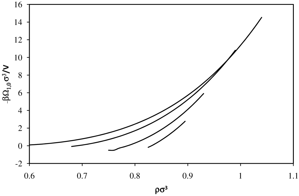
Figure 1: Classical grand potential or pressure, $-\beta\Omega_{1,0}\sigma^{3}/V=\beta p_{\mathrm{cl}}\sigma^{3}$, as a function of density for a Lennard-Jones model on liquid branch isotherms. The temperatures are $k_{\mathrm{B}}T/\epsilon=$ 0.5, 0.6, 0.8, and 1.0 from bottom to top, respectively.

Figure 1 shows the total classical grand potential for a Lennard-Jones model calculated in hypernetted chain approximation. The quantity plotted is equal to the pressure, $\beta p\sigma^{3}$. (Actually in this figure the virial pressure has been calculated rather than the grand potential in hypernetted chain approximation.)TDSM The curves represent the liquid branch of sub-critical isotherms. They terminate at the last point of convergence of the hypernetted chain algorithm, which correspond approximately to the gas and solid spinodal points. Negative values of the pressure correspond to metastable states. It can be seen that the pressure increases with increasing density, and that it increases with increasing temperature. The latter is a result of the reduction in weight of the attractive tail of the Lennard-Jones potential as the temperature is increased. As a comparison, the ideal gas classical pressure is equal to the density in these units and would be a straight line.

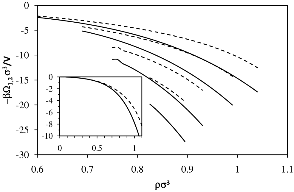
Figure 2: Non-commuting quantum correction to order $\hbar^{2}$, $-\beta\Omega_{1,2}\sigma^{3}/V$, as a function of density for a Lennard-Jones model of helium on liquid branch isotherms. Both sets of curves represent Eq. (4.20): the solid curves use only the pair distribution function (the final equality), and the dashed curves use the Kirkwood superposition approximation for the triplet distribution function (the penultimate equality). The temperatures are $k_{\mathrm{B}}T/\epsilon=$ 0.5, 0.6, 0.8, and 1.0 from bottom to top, respectively. Inset. Supercritical isotherm, $k_{\mathrm{B}}T/\epsilon=1.5$

Figure 2 shows the leading quantum correction due to the non-commutation of position and momentum. The quantity plotted, $-\beta\Omega_{1,2}\sigma^{3}/V$, which can be compared directly to the pressure, gives the quantum correction to ${\cal O}(\hbar^{2})$, which in fact is proportional to the thermal wave length squared, The calculations are for a Lennard-Jones model of helium. with mass $m=4.003\,$amu, potential well parameter $\epsilon/k_{\mathrm{B}}=10.22\,$K, and core parameter $\sigma=0.2556\,$nm.Sciver12 Again the hypernetted chain result for the radial distribution function is used. Classical simulations have previously been used to obtain the first quantum correction due to non-commutativity in argon and neon.Barker73 ; Singer84

The magnitude of the quantum correction shown in Fig. 2 increases with decreasing temperature. This is the opposite trend to that for the total pressure, Fig. 1, and so one sees that quantum effects become relatively more important at low temperatures, as one would expect. The fact that this quantum correction is negative means that the quantum effects due to non-commutativity of the position and momentum operators decreases the pressure compared to an otherwise equivalent classical system. For the lowest temperature and highest density here, the magnitude of the first quantum correction due to non-commutativity is larger than the total classical pressure itself. This suggests that it is necessary to include more terms in the series if the quantum correction due to non-commutativity is to be reliably obtained for low temperature liquid helium.

Figure 2 also tests the Kirkwood superposition approximation for $g^{(3)}$ (cf. Eq. (4.20)). One can see that the superposition approximation is reasonably accurate for this quantum correction at the highest temperature and lowest densities shown. As can be seen in the inset, at the supercritical temperature of $k_{\mathrm{B}}T/\epsilon=1.5$, the two calculations are within 10% for $\rho\sigma^{3}\lesssim 0.5$. However the superposition approximation significantly underestimates the magnitude of the correction at higher densities and at lower temperatures.

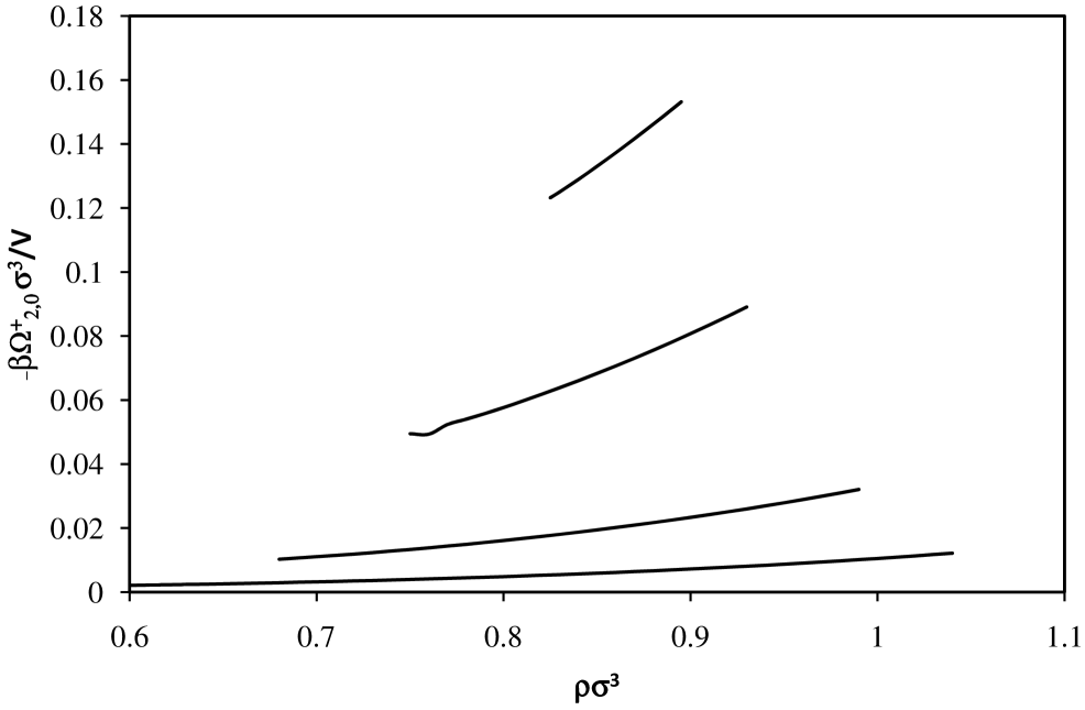
Figure 3: Dimer grand potential for bosons, $-\beta\Omega^{+}_{2,0}\sigma^{3}/V$, with all curves and parameters as in the preceding figure, except that the temperature increases from top to bottom.

Figure 3 shows the first quantum correction due to symmetrization, $-\beta\Omega^{+}_{2,0}\sigma^{3}/V$, again for helium. The data plotted is for bosons; the results for fermions are equal in magnitude and opposite in sign. The positive values in Fig. 3 indicate that particle symmetrization effects increase the pressure for bosons and decrease the pressure for fermions compared to a classical liquid at the same density. It can be seen that again the magnitude of the correction increases with decreasing temperature. However in this regime for helium, the correction due to symmetrization is about two orders of magnitude smaller than the correction due to non-commutativity. (At the highest density and lowest temperature shown, $\Omega^{+}_{2,0}\approx\Omega^{+}_{1,2}/200$.) Nevertheless the effect of quantum symmetrization is on the order of 10–20% of the total classical pressure, with it being relatively larger as the density is decreased or as the temperature is lowered.

This first quantum correction due to symmetrization is for a Lennard-Jones liquid about 3–4 times smaller than the same correction for an ideal gas. This reduction is due to the short-range repulsion between the Lennard-Jones particles, as discussed in §IV.2.1.

For helium, at $k_{\mathrm{B}}T/\epsilon=$ 0.5, the thermal wavelength is $\Lambda=1.51\sigma$, and at $k_{\mathrm{B}}T/\epsilon=$ 1.0, it is $\Lambda=1.07\sigma$. In these cases there is enough overlap between the Gaussian symmetrization factor and the non-zero part of the radial distribution function for the symmetrization quantum correction to be non-negligible.

For the case of argon, $m=39.948\,$amu, $\epsilon/k_{\mathrm{B}}=124.0\,$K, and $\sigma=0.3418\,$nm,Sciver12 the first quantum correction was found to be effectively zero. In this case, at $k_{\mathrm{B}}T/\epsilon=$ 0.5, the thermal wavelength is $\Lambda=0.103\sigma$. The radial distribution function $g(q)$ is approximately zero for $q\lesssim\sigma$, and the Gaussian factor that arises from symmetrization is effectively zero for $q\gtrsim\Lambda/\sqrt{2\pi}$. In the case of argon there is almost no overlap between the two. As the density is increased, the non-zero part of the radial distribution function shifts to smaller separations. But the classical pressure also rapidly increases, and it is difficult to see the quantum correction becoming relatively significant for argon. Higher densities have not been studied because the present hypernetted chain algorithm is unsuited for the solid phase.

The first quantum correction due to non-commutativity is proportional to the thermal wave length squared, and it about $200$ times smaller for argon than for helium at the lowest temperature shown.

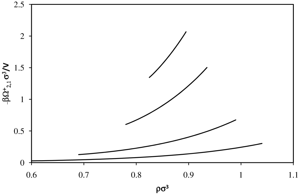
Figure 4: Dimer grand potential for bosons with first correction for non-commutativity, $-\beta\Omega^{+}_{2,1}\sigma^{3}/V$, with all curves and parameters as in the preceding figure.

Figure 4 shows the leading order quantum correction due to the combination of non-commutativity and symmetrization, Eq. (3.24). This is positive for bosons and negative for fermions. Interestingly enough, it is larger in magnitude than is the first correction for symmetrization alone (cf. Fig. 3). It is however smaller in magnitude than the first non-zero correction for non-commutativity alone (cf. Fig. 2). At low densities toward the liquid spinodal point, where the total classical pressure is close to zero or negative, this correction can exceed the total classical pressure. At the lowest temperature shown it is comparable to the total classical pressure along the whole liquid branch isotherm.

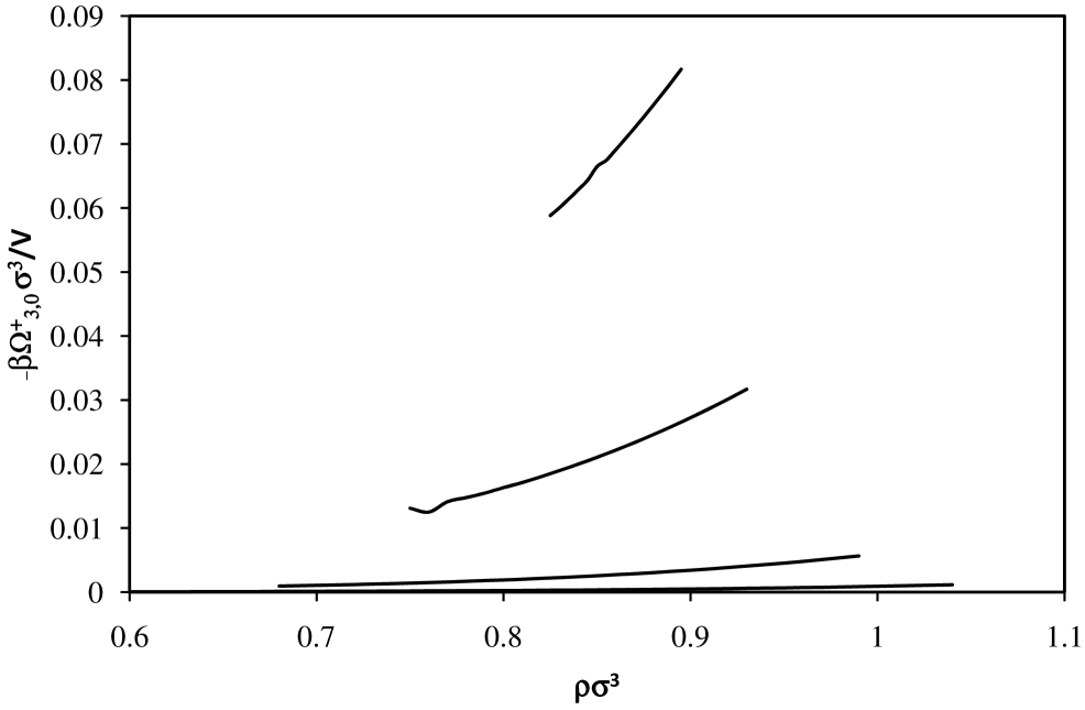
Figure 5: Trimer grand potential for bosons, $-\beta\Omega^{+}_{3,0}\sigma^{3}/V$, with all curves and parameters as in the preceding figure.

Figure 5 shows the trimer grand potential, to be again compared directly to the pressure $\beta p\sigma^{3}$. In this case the quantum correction is identical for bosons and for fermions. The fact that it is positive means that second order quantum effects increase the classical pressure. It should be cautioned that the quantitative results here depend on the accuracy of the Kirkwood superposition approximation (cf. the discussion of Fig. 2).

It can be seen that this second quantum correction due to symmetrization is about a factor of 2 smaller than the first quantum correction shown in Fig. 3 at the lowest temperature. At higher temperatures the second quantum correction is smaller than this in relative terms. These results allow the tentative conclusion that the loop expansion is rapidly converging, at least at these temperatures. Because the corrections alternate in sign for fermions, one might expect the series for them to be more slowly converging than for bosons.

V Conclusion

The quantum states that represent phase space identified here arise by taking an asymmetric expectation value of the Maxwell-Boltzmann operator. This involves two complete basis sets: plane waves, which localize particle momenta, and Gaussians, which localize particle positions. The consequent manipulations of the von Neumann trace for the partition function are formally exact.

The Maxwell-Boltzmann operator acting on a plane wave is here written as the exponential of an effective Hamiltonian, similar to an expression given by Wigner.Wigner32 A subsequent expansion gives the classical Maxwell-Boltzmann probability function times a series of terms involving powers of gradients of the potential energy, essentially the same as that given by Kirkwood.Kirkwood33 The classical average of these gives the quantum corrections due to the non-commutativity of the position and momentum operators. The present derivation is relatively simple and it appears straightforward to obtain the higher order terms in the expansion explicitly.

The particle interchange symmetrization of the wave function gives rise to an overlap factor in the grand partition function. This is expanded and re-summed, and the resultant permutation loop overlap factors are simple Gaussians in classical phase space. Again the terms in the series can be written as classical averages.

One piece of evidence for the validity of the formalism is the analysis of the ideal gas. In this system the quantum effects are due entirely to wave function symmetrization. The fact that the fugacity series for the pressure found here agrees with that given in standard textsPathria72 gives one confidence that the approach is fundamentally sound and free of algebraic errors.

A second piece of evidence is the comparison with the results of WignerWigner32 and KirkwoodKirkwood33 for the leading quantum correction due to non-commutativity (ie. neglecting wave function symmetrization). Despite the fact that the formulations of the actual quantum states for classical phase space are quite different, it turns out that the average of a function of position, and the average of the kinetic energy operator, are the same to leading order in the two approaches. However whereas WignerWigner32 and KirkwoodKirkwood33 give a phase space probability distribution, albeit a different one in each case, this appears to be precluded in the present theory.

The dual expansion obtained here appears computationally tractable. All the terms that appear can be expressed as classical equilibrium averages, and there is no need to compute eigenvalues, eigenfunctions, or explicitly symmetrized wave functions. Here liquid helium was modeled with a Lennard-Jones potential and the leading order corrections were obtained with the hypernetted chain approximation. No doubt in the future classical Monte Carlo or molecular dynamics simulations, in which the computational burden is ${\cal O}(N)$, could be used to obtain higher order corrections or to treat more challenging cases such as solid state or electronic systems. In the present calculations for liquid isotherms, quantum effects due to non-commutativity were found to be much larger than the effects due to wave function symmetrization. This is unlikely to be a general rule and it would be interesting to apply the present expansion to systems where symmetrization effects dominate.

Appendix A Exponential Expansion for the Quantum Weight Factor

In the text, §II.4, the quantum weight $W({\bf\Gamma})$, which arises from the non-commutativity of the momentum and position operators, was introduced. This was expanded in powers of $\hbar$, with the coefficients determined from a recursion relation that arises from the temperature derivative of the defining equation. The structure of the defining equation, Eq. (2.32), suggests that it may be useful to write

$$W({\bf\Gamma})\equiv e^{w({\bf\Gamma})}.$$ (A.1)

The reasons why it is better to deal with $w$ than $W$ will be discussed at the end of this appendix.

With this the temperature derivative of the defining equation (2.36) becomes

$$\frac{\partial w}{\partial\beta} = \frac{i\hbar}{m}e^{\beta U-w}{\bf p}\cdot\nabla\left\{e^{w-\beta U}\right\}+\frac{\hbar^{2}}{2m}e^{\beta U-w}\nabla^{2}\left\{e^{w-\beta U}\right\}$$ (A.2)

$$= \frac{i\hbar}{m}{\bf p}\cdot\nabla(w-\beta U)+\frac{\hbar^{2}}{2m}\left\{\rule{0.0pt}{11.38092pt}\nabla(w-\beta U)\cdot\nabla(w-\beta U)\right.$$

$$\left.\mbox{ }+\nabla^{2}(w-\beta U)\rule{0.0pt}{11.38092pt}\right\}.$$

One can expand $w$ in powers of Planck’s constant,

$$w\equiv\sum_{n=1}^{\infty}w_{n}\hbar^{n}.$$ (A.3)

This begins at $n=1$ because the classical part must vanish, $W(\hbar=0)=1\Rightarrow w(\hbar=0)=0$. Also $W(\beta=0)=1\Rightarrow w_{n}(\beta=0)=0$.

The first coefficient satisfies

$$\frac{\partial w_{1}}{\partial\beta}=\frac{-i\beta}{m}{\bf p}\cdot\nabla U,$$ (A.4)

which gives

$$w_{1}=\frac{-i\beta^{2}}{2m}{\bf p}\cdot\nabla U.$$ (A.5)

The second coefficient satisfies

$$\frac{\partial w_{2}}{\partial\beta} = \frac{i}{m}{\bf p}\cdot\nabla w_{1}+\frac{1}{2m}\left\{\rule{0.0pt}{11.38092pt}\beta^{2}\nabla U\cdot\nabla U-\beta\nabla^{2}U\rule{0.0pt}{11.38092pt}\right\},$$

which gives

$$w_{2} = \frac{\beta^{3}}{6m^{2}}{\bf p}{\bf p}:\nabla\nabla U+\frac{1}{2m}\left\{\rule{0.0pt}{11.38092pt}\frac{\beta^{3}}{3}\nabla U\cdot\nabla U-\frac{\beta^{2}}{2}\nabla^{2}U\rule{0.0pt}{11.38092pt}\right\}.$$

In general for $n>2$

$$\frac{\partial w_{n}}{\partial\beta} = \frac{i}{m}{\bf p}\cdot\nabla w_{n-1}+\frac{1}{2m}\sum_{j=0}^{n-2}\nabla w_{n-2-j}\cdot\nabla w_{j}$$ (A.8)

$$\mbox{ }-\frac{\beta}{m}\nabla w_{n-2}\cdot\nabla U+\frac{1}{2m}\nabla^{2}w_{n-2}.$$

For $n=3$ one can show that

$$w_{3} = \frac{i\beta^{4}}{24m^{3}}{\bf p}{\bf p}{\bf p}\vdots\nabla\nabla\nabla U+\frac{5i\beta^{4}}{24m^{2}}{\bf p}(\nabla U):\nabla\nabla U$$ (A.9)

$$\mbox{ }-\frac{i\beta^{3}}{6m^{2}}{\bf p}\cdot\nabla\nabla^{2}U,$$

and for $n=4$ one has

$$w_{4} = \frac{-i^{4}\beta^{5}}{5!m^{4}}({\bf p}\cdot\nabla)^{4}U-\frac{\beta^{5}}{30m^{3}}(\nabla U){\bf p}{\bf p}\vdots\nabla\nabla\nabla U$$

$$\mbox{ }-\frac{\beta^{5}}{15m^{2}}(\nabla U)(\nabla U):\nabla\nabla U+\frac{\beta^{4}}{16m^{2}}\nabla U\cdot\nabla\nabla^{2}U$$

$$\mbox{ }+\frac{\beta^{4}}{48m^{3}}{\bf p}{\bf p}:\nabla\nabla\nabla^{2}U+\frac{\beta^{4}}{48m^{2}}\nabla^{2}(\nabla U\cdot\nabla U)$$

$$\mbox{ }-\frac{\beta^{3}}{24m^{2}}\nabla^{2}\nabla^{2}U-\frac{\beta^{5}}{40m^{3}}({\bf p}\cdot\nabla\nabla U)\cdot({\bf p}\cdot\nabla\nabla U).$$

Dealing with $w$ has arguably two advantages over $W$. First, experience shows that the expansion of an exponent converges more quickly than the expansion of an exponential. For example keeping only the terms $w_{1}$ and $w_{2}$ encompasses the terms $W_{1}$ and $W_{2}$, and an infinite number of higher order terms besides. Second, $w$ is an extensive variable, as can be seen by inspection, whereas $W$ is a sum of terms of every power of the system size.

Appendix B Non-Extensive Quantum Weight

The point made at the end of the preceding appendix —that the quantum weight for non-commutativity is not extensive— has some significant consequences for the analysis in the text. Although the exponent $w$ may be expanded in powers of $\hbar$, the fact that it is extensive means that one cannot realistically linearize the exponential to obtain a useful expansion of $W$ in powers of $\hbar$ without further work.

That $w$ is extensive can be seen from the original defining equation,

$$e^{-\beta\hat{\tilde{\cal H}}({\bf\Gamma})}1=e^{-\beta{\cal H}({\bf\Gamma})+w({\bf\Gamma})}.$$ (B.1)

Since the operator exponent on the left hand side is extensive, then so too must be the function exponent on the right hand side. Alternatively, this can also be seen from the temperature derivative,

$$\frac{\partial w}{\partial\beta} = \frac{i\hbar}{m}{\bf p}\cdot\nabla(w-\beta U)+\frac{\hbar^{2}}{2m}\left\{\rule{0.0pt}{11.38092pt}\nabla(w-\beta U)\cdot\nabla(w-\beta U)\right.$$ (B.2)

$$\left.\mbox{ }+\nabla^{2}(w-\beta U)\rule{0.0pt}{11.38092pt}\right\}.$$

On the right hand side each element of the gradient operator acts on a single particle. Hence the scalar product with the gradient operator is extensive.

B.1 Second Order Analysis

In the first instance one can focus on the monomer grand potential. (A completely analogous argument can be applied to the loop grand potentials for $l\geq 2$.) The monomer grand potential is $\Omega_{1}=-k_{\mathrm{B}}T\ln\Xi_{1,w}$, with the monomer grand partition function being

$$\Xi_{1,w}=\sum_{N}\frac{z^{N}}{N!h^{3N}}\int\mathrm{d}{\bf\Gamma}\;e^{-\beta{\cal H}({\bf\Gamma})}e^{w({\bf\Gamma})}.$$ (B.3)

The difference between the monomer grand potential and the classical grand potential is essentially just the logarithm of the classical average of the quantum weight due to non-commutativity

$$-\beta[\Omega_{1}-\Omega_{1,0}]=\ln\left<e^{w}\right>_{1,0}.$$ (B.4)

The left hand side is extensive, which is to say that it scales with the volume of the system. Hence the grand potential density is independent of the size of the system. Since $w\propto V$, and since $w(\hbar=0)=0$, one can suppose that there exists a volume small enough that $w\ll 1$. For such a volume one can expand the exponential to obtain

$$-\beta[\Omega_{1}-\Omega_{1,0}]$$ (B.5)

$$= \ln\left<e^{w}\right>_{1,0}$$

$$= \ln\left<1+w+\frac{1}{2}w^{2}+\ldots\right>_{1,0}$$

$$= \left<w\right>_{1,0}+\frac{1}{2}\left<[w-\left<w\right>_{1,0}]^{2}\right>_{1,0}+\ldots$$

The first term on the right hand side is extensive. The second term, as the fluctuation of an extensive variable, is also extensive. Presumably, so are the higher order terms (see §B.2.2). Having obtained the final result, one can now allow the volume to become as large as desired.

B.1.1 Explicit Second Order Result

The first order correction vanishes, $\Omega_{1,1}=\hbar\left<w_{1}\right>_{1,0}=0$, because $w_{1}$ is odd in ${\bf p}$. The second order correction is given by

$$-\beta\Omega_{1,2}$$ (B.6a)

$$= \hbar^{2}\left<\frac{1}{2}w_{1}^{2}+w_{2}\right>_{1,0}$$

$$= \hbar^{2}\left<\frac{-1}{2}\frac{\beta^{4}}{4m^{2}}({\bf p}\cdot\nabla U)^{2}+\frac{\beta^{3}}{6m^{2}}{\bf p}{\bf p}:\nabla\nabla U\right.$$

$$\mbox{ }\left.+\frac{\beta^{3}}{6m}\nabla U\cdot\nabla U-\frac{\beta^{2}}{4m}\nabla^{2}U\right>_{1,0}$$

$$= \hbar^{2}\left<\frac{-1}{2}\frac{\beta^{4}}{4m^{2}}mk_{\mathrm{B}}T\nabla U\cdot\nabla U+\frac{\beta^{3}}{6m^{2}}mk_{\mathrm{B}}T\nabla^{2}U\right.$$

$$\mbox{ }\left.+\frac{\beta^{3}}{6m}\nabla U\cdot\nabla U-\frac{\beta^{2}}{4m}\nabla^{2}U\right>_{1,0}$$

$$= \hbar^{2}\left<\frac{\beta^{3}}{24m}\nabla U\cdot\nabla U-\frac{\beta^{2}}{12m}\nabla^{2}U\right>_{1,0}$$

$$= \left<\frac{-\hbar^{2}\beta^{2}}{24m}\nabla^{2}U\right>_{1,0}.$$ (B.6b)

This is the same as the result given in the text, which in turn agrees with that given by WignerWigner32 and by Kirkwood.Kirkwood33 The present derivation is more satisfactory than the others because it explicitly takes into account extensivity. Also, the higher order terms lend themselves to practical implementation either as an expansion, or else as the original exponential combined with umbrella sampling.

Table 1: Quantum correction for monomers due to non-commutativity, ${-\beta\Omega_{1,2}\sigma^{3}}/{V}$, for Lennard-Jones models of neon and helium at $k_{\mathrm{B}}T/\epsilon=1.5$ and $\rho\sigma^{3}=0.5$. For comparison, the classical pressure is $0.27575\pm 0.00080$. The results are from Metropolis Monte Carlo simulations, with $50\times 100$ configurations for averages, 20 trial steps per atom between averages, acceptance rate $\approx 50\%$, $R_{\mathrm{cut}}=3.5\sigma$, tail correction added, and no umbrella sampling, for a canonical system with $N=$250, 500, or 1000. The statistical error (68% confidence level) in the final digit is shown in parenthesis.

	250	500	1000
	Neon
a	-0.03484(8)	-0.03500(5)	-0.03504(3)
b	-0.03475(5)	-0.03500(3)	-0.03498(2)
d	-0.0256(6)	-0.0285(3)	-0.0300(2)
	Helium
a	-0.730(2)	-0.734(1)	-0.7346(7)
b	-0.728(1)	-0.7338(7)	-0.7333(5)
d	-.38(1)	-0.518(7)	-

The justification for the final equality is an integration by parts, assuming that surface integrals are negligible. As can be seen from the Table 1, computer simulations confirm the validity of this assumption. The results labeled d correspond to averaging the full exponential without umbrella sampling, ${-\beta\Omega_{1,2}^{d}}=\ln\left<\exp[\hbar w_{1}+\hbar^{2}w_{2}]\right>_{1,0}$. It can be seen that this approach has a significant system size dependence, and that in the case of helium numerical overflow occurs for the largest size studied. For helium at this state point, the hypernetted chain approximation used in the text gives $\beta p\sigma^{3}=0.391$, ${-\beta\Omega_{1,2}^{a}\sigma^{3}}/{V}=-0.741$, and ${-\beta\Omega_{1,2}^{b}\sigma^{3}}/{V}=-0.790$.

B.1.2 Tail Correction

The Laplacian of the tail of the Lennard-Jones potential is

$$\nabla^{2}U_{\mathrm{tail}} = \sum_{j\neq k}\left\{u_{\mathrm{tail}}^{\prime\prime}(q_{jk})+\frac{2}{q_{jk}}u_{\mathrm{tail}}^{\prime}(q_{jk})\right\}$$ (B.7)

$$= -4\epsilon\sum_{j\neq k}\left\{\frac{42\sigma^{6}}{q_{jk}^{8}}-\frac{12\sigma^{6}}{q_{jk}^{8}}\right\}.$$

Hence the tail of the quantum correction is

$$-\beta\Omega_{1,2}^{\mathrm{tail}} = \frac{-\hbar^{2}\beta^{2}}{24m}\left<\nabla^{2}U_{\mathrm{tail}}\right>_{1,0}$$ (B.8)

$$= \frac{-\hbar^{2}\beta^{2}}{24m}4\pi\rho^{2}V(-4\epsilon)\int_{q_{\mathrm{cut}}}^{\infty}\mathrm{d}q\,q^{2}\frac{30\sigma^{6}}{q^{8}}$$

$$= \frac{-4\pi\rho^{2}V\hbar^{2}\beta^{2}}{24m}(-4\epsilon)\frac{6\sigma^{6}}{q^{5}_{\mathrm{cut}}}.$$

B.2 Higher Order Analysis

B.2.1 Fourth Order Correction

The classical fluctuation of the weight exponent $w({\bf\Gamma})$ is

$$\Delta_{w}\equiv w-\left<w\right>_{1,0}.$$ (B.9)

Define a phase space constant that is a series of averages of powers of the fluctuation

$$D(\Delta_{w}) \equiv \left<w\right>_{1,0}+\frac{1}{2}\left<\Delta_{w}^{2}\right>_{1,0}+\frac{1}{3!}\left<\Delta_{w}^{3}\right>_{1,0}$$ (B.10)

$$\mbox{ }+\frac{1}{4!}\left<\Delta_{w}^{4}\right>_{1,0}-\frac{1}{8}\left<\Delta_{w}^{2}\right>_{1,0}^{2}.$$

This is constant in phase space, and so it can be taken in and out of averages. The average of the exponential of $w$ less this particular constant is

$$\left<e^{w-D(\Delta_{w})}\right>_{1,0}$$ (B.11)

$$= \left<\exp\left\{\Delta_{w}-\frac{1}{2}\left<\Delta_{w}^{2}\right>_{1,0}-\frac{1}{3!}\left<\Delta_{w}^{3}\right>_{1,0}\right.\right.$$

$$\left.\left.\mbox{ }-\frac{1}{4!}\left<\Delta_{w}^{4}\right>_{1,0}+\frac{1}{8}\left<\Delta_{w}^{2}\right>_{1,0}^{2}\right\}\right>_{1,0}$$

$$= 1+\left<\Delta_{w}\right>_{1,0}-\frac{1}{2}\left<\Delta_{w}^{2}\right>_{1,0}-\frac{1}{3!}\left<\Delta_{w}^{3}\right>_{1,0}-\frac{1}{4!}\left<\Delta_{w}^{4}\right>_{1,0}$$

$$\mbox{ }+\frac{1}{8}\left<\Delta_{w}^{2}\right>_{1,0}^{2}+\frac{1}{2}\left<\left[\Delta_{w}-\frac{1}{2}\left<\Delta_{w}^{2}\right>_{1,0}\right]^{2}\right>_{1,0}$$

$$\mbox{ }+\frac{1}{3!}\left<\left[\Delta_{w}-\frac{1}{2}\left<\Delta_{w}^{2}\right>_{1,0}\right]^{3}\right>_{1,0}+\frac{1}{4!}\left<\Delta_{w}^{4}\right>_{1,0}+\ldots$$

$$= 1+\left<{\cal O}(\Delta_{w}^{5})\right>_{1,0}.$$

This enables expansions to ${\cal O}(\hbar^{4})$ to be obtained relatively painlessly. For example, the monomer potential is

$$e^{-\beta[\Omega_{1}-\Omega_{1,0}]} = \frac{\Xi_{1}}{\Xi_{1,0}}$$ (B.12)

$$= \left<e^{w}\right>_{1,0}$$

$$= e^{D(\Delta_{w})}\left<e^{w-D(\Delta_{w})}\right>_{1,0}$$

$$= e^{D(\Delta_{w})}\left[1+\left<{\cal O}(\Delta_{w}^{5})\right>_{1,0}\right].$$

Hence

$$-\beta\Omega_{1}=-\beta\Omega_{1,0}+D(\Delta_{w})+{\cal O}(h^{5}),$$ (B.13)

assuming that $w$ itself has been obtained to at least fourth order.

More generally, for obtaining averages and loop potentials, for a phase function $A$ define the fluctuation

$$\Delta_{Aw}\equiv w-\left<w\right>_{1,A}\equiv w-\frac{\left<Aw\right>_{1,0}}{\left<A\right>_{1,0}}.$$ (B.14)

Define the phase space constant

$$D(\Delta_{Aw}) \equiv \left<w\right>_{1,A}+\frac{1}{2}\left<\Delta_{Aw}^{2}\right>_{1,A}+\frac{1}{3!}\left<\Delta_{Aw}^{3}\right>_{1,A}$$ (B.15)

$$\mbox{ }+\frac{1}{4!}\left<\Delta_{Aw}^{4}\right>_{1,A}-\frac{1}{8}\left<\Delta_{Aw}^{2}\right>_{1,A}^{2}.$$

One has

$$\left<Ae^{w}\right>_{1,0} = \left<A\right>_{1,0}\left<e^{w}\right>_{1,A}$$ (B.16)

$$= \left<A\right>_{1,0}e^{D(\Delta_{Aw})}\left<e^{w-D(\Delta_{Aw})}\right>_{1,A}$$

$$= \left<A\right>_{1,0}e^{D(\Delta_{Aw})}[1+{\cal O}(\hbar^{5})].$$

This result gives directly the monomer average of of a function (operator) of the position configuration $A({\bf q})$.

For the loop potential one need only take $A\Rightarrow X^{(l)}$. With this the loop potential $l\geq 2$ can be expanded as

$$-\beta\Omega_{l} = \frac{\left<X^{(l)}e^{w}\right>_{1,0}}{\left<e^{w}\right>_{1,0}}$$ (B.17)

$$= \frac{\left<X^{(l)}\right>_{1,0}\left<e^{w}\right>_{1,X^{(l)}}}{\left<e^{w}\right>_{1,0}}$$

$$= \left<X^{(l)}\right>_{1,0}e^{D(\Delta_{X^{(l)}w})-D(\Delta_{w})}+{\cal O}(h^{5}).$$

The full average of a function of position is given by Eq. (II.7.1) (with $W\Rightarrow e^{w}$),

$$\left<O({\bf r})\right>_{\mu,V,T}$$

$$= \frac{\langle Oe^{w}\rangle_{1,0}}{\langle e^{w}\rangle_{1,0}}\prod_{l=2}^{\infty}\exp\left<X^{(l)}\left[\frac{Oe^{w}}{\langle Oe^{w}\rangle_{1,0}}-\frac{e^{w}}{\langle e^{w}\rangle_{1,0}}\right]\right>_{1,0}.$$

One need only replace $A$ by an appropriate function in each average on the right hand side to obtain a relatively simple expression that is valid to ${\cal O}(h^{4})$.

B.2.2 Gaussian Form

One can assume, with a confidence approaching certainty in the thermodynamic limit, that the value of an extensive physical variable is Gaussian distributed.

In the present case this means that

$$\wp(w)=\frac{1}{\sqrt{2\pi\sigma^{2}}}e^{-\Delta_{w}^{2}/2\sigma^{2}},$$ (B.19)

where $\Delta_{w}\equiv w-\langle w\rangle_{1,0}$ and $\sigma=\sqrt{\langle\Delta_{w}^{2}\rangle_{1,0}}$. Hence

$$\left\langle e^{w}\right\rangle_{1,0} = \int\mathrm{d}w\;\wp(w)e^{w}$$ (B.20)

$$= \frac{1}{\sqrt{2\pi\sigma^{2}}}\int\mathrm{d}w\;e^{\langle w\rangle_{1,0}}e^{-(\Delta_{w}-\sigma^{2})^{2}/2\sigma^{2}}e^{\sigma^{2}/2}$$

$$= e^{\langle w\rangle_{1,0}}e^{\langle\Delta_{w}^{2}\rangle_{1,0}/2}.$$

This is consistent with the leading terms derived explicitly above. Obviously one can replace the subscript $1,0$ by $1,A$, and $\Delta_{w}$ by $\Delta_{Aw}$, as appropriate.

References

• (1) Hernando, A. and Vinìček, J. (2013), ‘Imaginary-Time Nonuniform Mesh Method for Solving the Multidimensional Schrödinger Equation: Fermionization and Melting of Quantum Lennard-Jones Crystals’, arXiv:1304.8015v2 [quant-ph].
• (2) Georgescu, I. and Mandelshtam, V. A. (2011), ‘A Fast Variational Gaussian Wave-Packet Method: Size-Induced Structural Transitions in Large Neon Clusters’, arXiv:1107.3330v2 [cond-mat.stat-mech].
• (3) Allen, M. P. and Tildesley, D. J. (1987), Computer Simulations of Liquids, (Oxford University Press, Oxford).
• (4) Attard, P. (2012), Non-Equilibrium Thermodynamics and Statistical Mechanics: Foundations and Applications, (Oxford University Press, Oxford).
• (5) Wigner, E. (1932), ‘On the Quantum Correction for Thermodynamic Equilibrium’ Phys. Rev. 40, 749.
• (6) Kirkwood, J. (1933), ‘Quantum Statistics of Almost Classical Particles’, Phys. Rev. 44, 31.
• (7) Groenewold, H. J. (1946), ‘On the Principles of Elementary Quantum Mechanics’, Physica, 12, 405.
• (8) Moyal, J. E. (1949), ‘Quantum Mechanics as a Statistical Theory’, Proc. Cambridge Phil. Soc. 45, 99.
• (9) Zachos, C., Fairlie, D., and Curtright, T. (2005), Quantum Mechanics in Phase Space, (World Scientific, Singapore).
• (10) Barnett, S. M. and Radmore, P. M. (2003), Methods in Theoretical Quantum Optics, (Oxford University Press, Oxford).
• (11) Gerry, C. and Knight, P. (2005), Introductory Quantum Optics, (Cambridge University Press, Cambridge).
• (12) Najarbashi, G. and Mirzaei, S. (2016), ‘One-Mode Wigner Quasi-Probability Distribution Function for Entangled Coherent States Generated by Beam Splitter and Cavity QED’, arXiv:1601.00143v2 [quant-ph].
• (13) Park, J. and Nha, H. (2016), ‘Demonstrating Nonclassicality and Non-Gaussianity of Single-Mode Fields: Bell-Type Tests Using Generalized Phase-Space Distributions’, arXiv:1601.00279v1 [quant-ph].
• (14) Braunstein S. L. and van Loock, P. (2005), ‘Quantum Information with Continuous Variables’, Rev. Mod. Phys. 77, 513.
• (15) Weedbrook, C., Pirandola, S., Garcí a-Patrón, R., Cerf, N. J., Ralph, T. C., Shapiro, J. H., and Lloyd, S. (2012), ‘Gaussian Quantum Information’, Rev. Mod. Phys. 84, 621.
• (16) Praxmeyer, L. and Wódkiewicz, K. (2002) ‘Quantum Interference in the Kirkwood-Rihaczek Representation’ arXiv:quant-ph/0207127v1.
• (17) Dishlieva, K. G. (2008), ‘Kirkwood and Wigner Distribution Functions: Graphical Imaging’, Int. J. Pure Appl. Math. 42, 583.
• (18) Davies, E. B. (1976), Quantum Theory of Open Systems, (Academic Press, London).
• (19) Zeh, H. D. (2001), The Physical Basis of the Direction of Time, (Springer, Berlin, 4th ed.).
• (20) Breuer, H.-P. and Petruccione, F. (2002), The Theory of Open Quantum Systems, (Oxford University Press, Oxford).
• (21) Zurek, W. H. (2003), ‘Decoherence, Einselection, and the Quantum Origins of the Classical’, Rev. Mod. Phys. 75, 715; arXiv:quant-ph/0105127v3.
• (22) Weiss, U. (2008), Quantum Dissipative Systems, (World Scientific, Singapore, 3rd Ed.).
• (23) Attard, P. (2013), ‘Quantum Statistical Mechanics. I. Decoherence, Wave function Collapse, and the von Neumann Density Matrix’, arXiv:1401.1786v1.
• (24) Attard, P. (2015), Quantum Statistical Mechanics: Equilibrium and Non-Equilibrium Theory from First Principles, (IOP Publishing, Bristol).
• (25) von Neumann, J. (1927), ‘Wahrscheinlichkeitstheoretischer Aufbau der Quantenmechanik’, Göttinger Nachrichten 1, 245.
• (26) Messiah, A. (1961), Quantum Mechanics, (North-Holland, Amsterdam, Vols I and II).
• (27) Merzbacher, E. (1970), Quantum Mechanics, (Wiley, New York, 2nd edn).
• (28) Attard, P. (2016), ‘Expansion for Quantum Statistical Mechanics Based on Wave Function Symmetrization’, arXiv:1603.07757v2.
• (29) Pathria, R. K. (1972), Statistical Mechanics, (Pergamon Press, Oxford).
• (30) KirkwoodKirkwood33 appears to use the notation ${\bf r}_{k}=\{r_{kx},r_{ky},r_{kz}\}=\{q_{k},q_{N+k},q_{2N+k}\}$. In this $r$ is the same as $q$, and neither distinguishes position coordinates from position configurations.
• (31) Attard, P. (2002), Thermodynamics and Statistical Mechanics: Equilibrium by Entropy Maximisation, (Academic Press, London).
• (32) Abramowitz, M. and Stegun, I. A. (1965), Handbook of Mathematical Functions, (Dover, New York).
• (33) Attard, P. (1989), ‘Spherically Inhomogeneous Fluids. I. Percus-Yevick Hard-Spheres: Osmotic Coefficients and Triplet Correlations.’ J. Chem. Phys. 91, 3072.
• (34) Attard, P. (1991), ‘Lennard-Jones Bridge Functions and Triplet Correlation Functions’, J. Chem. Phys. 95, 4471.
• (35) van Sciver, S. W. (2012), Helium Cryogenics, (Springer, New York, 2nd ed.).
• (36) Barker, J. A. and Klein, M. L. (1973), ‘Monte Carlo Calculations for Solid and Liquid Argon’, Phys. Rev. B 7, 4707.
• (37) Singer, J. V. L. and Singer, K. (1984), ‘Molecular Dynamics Based on the First Order Quantum Correction in the Wigner-Kirkwood Expansion’, CCP5 Quarterly, 14, 24.
• (38) Attard, P. (1992), ‘Simulation Results for a Fluid with the Axilrod-Teller Triple Dipole Potential’, Phys. Rev. A. 45, 5649.