Orientation Statistics and Quantum Information

Abstract

Motivated by the engineering applications of uncertainty quantification, in this work we draw connections between the notions of random quantum states and operations in quantum information with probability distributions commonly encountered in the field of orientation statistics. This approach identifies natural probability distributions that can be used in the analysis, simulation, and inference of quantum information systems. The theory of exponential families on Stiefel manifolds provides the appropriate generalization to the classical case, and fortunately there are many existing techniques for inference and sampling that exist for these distributions. Furthermore, this viewpoint motivates a number of additional questions into the convex geometry of quantum operations relative to both the differential geometry of Stiefel manifolds as well as the information geometry of exponential families defined upon them. In particular, we draw on results from convex geometry to characterize which quantum operations can be represented as the average of a random quantum operation.

I Introduction

Consider some arbitrary classical (i.e., non-quantum) experimental procedure, wherein experiments are performed and measurements are taken to quantify some characteristic of some component. Suppose this component is to be included as sub-component of a larger system and an engineer is charged with performing an analysis (likely via computer simulation) of how variability of the sub-components affects the overall system performance. Such studies are commonly denoted sensitivity analysis, risk analysis, or uncertainty quantification Iman and Helton (1988); Saltelli et al. (2000) and such techniques are of practical concern in a variety of contexts. Suppose the engineer tracks down the experimental results for a given component (e.g., length tolerances for some packaging) and is able to obtain the sample data generated by the experimentalist, or more likely, the reported mean $\mu$ and variance $\sigma^{2}$. In either case, it is likely that the engineer will model the distribution of the characteristic using the normal distribution $\mathcal{N}(\mu,\sigma^{2})$, and indeed, there is mathematical reasoning to do so Jaynes (1957), beyond any computational reasons for doing so. The engineer might use samples from this distribution as part of a Monte Carlo analysis, or perhaps the functional form of the probability distribution function can be used as part of a closed-form analysis.

A similar situation exists in quantum information, but it is often unremarked. On one hand, the evolution of an open quantum system can often be treated as a noisy evolution, through the stochastic Liouville equation Kubo (1963). This type of description applies to some of the most common types of qubits and their predominant decoherence mechanisms (see, e.g. Refs. Kubo (1957); Schulten and Wolynes (1978); Ernst et al. (1987); Schneider and Milburn (1998); Grigorescu (1998); Abergel and Palmer (2003); Cheng and Silbey (2004); Wilhelm et al. (2007)). On the other hand, especially in the context of quantum gates or circuits, we speak of “the superoperator” or “the error channel” for a given quantum operation, and not a stochastic process. Unlike the classical case, it is impossible to recover the quantum operation associated with an individual quantum trajectory, only measurements collected at the end of an experiment, which individually contain only partial information about the average quantum channel that generated the collections of measurements. Thus, techniques for converting sets of quantum measurements into estimates of quantum states or channels, called tomography, are essentially computing estimates of the average quantities of interest, in much the same way that descriptive statistics such as the mean and variance are used in classical contexts. This suggests that a rigorous statistical approach must be developed in order to develop accurate assessments of the impacts of noise and imperfections on quantum systems, when only sample averages of an underlying probability distribution are available.

Here, we develop such a statistical approach applicable to quantum information by showing the relationships between a number of probability distributions common in the field of directional or orientation statistics Mardia and Jupp (2009); Chikuse (2012), but somewhat obscure outside of this field, and a number of relevant structures in quantum information. In particular, we relate the parameters of these distributions to certain forms of quantum operations. The hope is that these distributions can be used both in closed-form and Monte Carlo analysis in the simulation of quantum circuits, as well a providing additional foundation for different inference problems concerning quantum systems.

In the discussion below, we first cover a number of relevant forms of quantum operations that we will later draw connections to from the field of orientation statistics. Next, we introduce the concept of an exponential family, which is a geometric concept that generalizes many of the familiar properties of normal random variables, such as the sufficiency of the sample mean and variance fully describing the sampled data, as well as the maximum entropy property that the normal distribution exhibits among all random variables with a fixed variance. The preliminary discussion is concluded by a brief overview of Stiefel manifolds, which will be the sample space (instead of Euclidean space) on which the relevant probability distributions will be defined.

I.1 CPTP Maps

In quantum information, a quantum state is represented by a density operator $\rho$, where $\rho\in\mathbb{C}^{N\times N}$ is a positive semi-definite, Hermitian matrix with $\operatorname{Tr}(\rho)=1$ Nielsen and Chuang (2010). Quantum operations are then completely positive, trace-preserving (CPTP) maps Nielsen and Chuang (2010). Here, we will make the additional assumption that the quantum maps of interest map to density operators of the same dimension as the input dimension, but this can be generalized. Below we will summarize some relevant properties and equivalent representations of CPTP maps that will help to draw the connection to the field of orientation statistics. More information about various forms of CPTP maps can be found in e.g. Fujiwara and Algoet (1999); Bruzda et al. (2009); Wood et al. (2014).

Choi’s theorem on completely positive (CP) maps Choi (1975) states that any CP map $\Phi(\rho)$ can be written in the Kraus form

$$\Phi(\rho)=\sum_{i=1}^{m}A_{i}\rho A_{i}^{\dagger}$$ (1)

where $A_{i}\in\mathbb{C}^{N\times N}$ and $m$ is said to be the Kraus rank of the map $\Phi$ and $m\leq N^{2}$. The added characteristic of trace preserving (TP) is equivalent to $\sum_{i}A_{i}^{\dagger}A_{i}\triangleq\mathbbm{1}_{N}$. Note that the Kraus form is not unique, that is, different sets of Kraus operators $A_{i}$ can create equivalent maps.

Let $|\cdot\rangle\rangle$ denote the vectorization operator, and $\langle\langle\cdot|=|\cdot\rangle\rangle^{\dagger}$. From the Kraus form, two additional representations of CPTP maps can be defined, the Choi matrix form

$$\Lambda=\sum_{i=1}^{m}|A_{i}\rangle\rangle\langle\langle A_{i}|\,,$$ (2)

and the Liouvillian superoperator (or dynamical matrix form)

$$\mathcal{L}=\sum_{i=1}^{m}A_{i}^{*}\otimes A_{i}\,,$$ (3)

where $*$ denotes entry-wise conjugation, not conjugate transposition ($\dagger$). These forms are of course equivalent and are related by a reshuffling involution Bruzda et al. (2009); Wood et al. (2014).

Let $\operatorname{Tr}_{2}$ denote the partial trace over the second Hilbert space in a composite system, so that $\operatorname{Tr}_{2}(A\otimes B)=A$. The TP property implies that $\operatorname{Tr}_{2}(\Lambda)=\mathbbm{1}_{N}$ (and thus $\operatorname{Tr}(\Lambda)=N$) and it is obvious from the form in (2) that $\Lambda$ is a positive semi-definite Hermitian matrix. As (2) has the same functional form as a density operator on $\mathbb{C}^{N^{2}\times N^{2}}$, there is an isomorphism between $\Lambda/N$ and density operators on the higher dimensional space $N^{2}$, called the Jamiołkowski isomorphism Jamiołkowski (1972). Since $\Lambda$ is a Hermitian positive semi-definite matrix, we can diagonalize it as $\Lambda=KDK^{\dagger}$ where $K$ is a unitary matrix (in particular, its columns are orthonormal) and $D$ is a diagonal matrix whose entries $D_{ii}\in[0,N]$ and $\sum D_{ii}=N$. Letting $|K_{i}\rangle\rangle$ denote the $i$th column of the above decomposition, $\Lambda$ can be used to define “canonical” Kraus operators $\sqrt{D_{ii}}K_{i}$.

While $\Lambda$ enjoys a number of useful structural properties, the Liouvillian superoperator is convenient for the propagation of state, as $\mathcal{L}(\rho)=\mathcal{L}|\rho\rangle\rangle$. In this work, the primary use of the superoperator will be as it relates to the Pauli transfer matrix or affine form Fujiwara and Algoet (1999). For a single qubit system ($N=2$), the Pauli transfer matrix is the Liouvillian superoperator expressed in the basis spanned by the vectorized Pauli matrices $|\sigma_{I}\rangle\rangle$, $|\sigma_{X}\rangle\rangle$, $|\sigma_{Y}\rangle\rangle$, $|\sigma_{Z}\rangle\rangle$. Higher dimensional analogues exist Fujiwara and Algoet (1999), but the key concept is that states $\rho$ (in say, the computational basis) are mapped to Bloch vectors $\varphi\in\mathbb{R}^{N^{2}-1}$ with $||\varphi||_{2}\leq 1$ and unitary quantum operations are represented as rotations (elements of $SO(N^{2}-1)$) of $\varphi$ along a hypersphere. The affine form of general CPTP maps can include two rotation components, a contraction component, and linear shift, but the focus here will be on affine representations of unitary operations.

I.2 Sufficient Statistics and Exponential Families

A probability distribution $p(x;\theta)$ parameterized by $\theta$ is said to be an exponential family if $p(x;\theta)$ can be expressed as

$$p(x;\theta)=\exp(\langle\theta,T(x)\rangle-\psi(\theta)+\kappa(x))\,,$$ (4)

where

• $\theta$ are the natural parameters

• $T(x)$ are the sufficient statistics Koopman (1936); Pitman (1936), typically linearly independent

• $\psi(\theta)$ is the log-normalizer which causes $p(x;\theta)$ to integrate to one

• $k(x)$ is the carrier measure that determines the support of the distribution, for example on the positive reals or some manifold embedded in Euclidean space

Exponential families play a prominent role in statistics Amari and Nagaoka (2007); Barndorff-Nielsen (2014), particularly in the context of maximum-likelihood estimation. Many common distributions such as Gaussian, exponential, Bernoulli, etc., are exponential families. Two basic facts of exponential families motivate their study here. The first is that the so-called expectation parameters $\eta$ of a probability distribution are defined by $\eta=E_{p(x;\theta)}[T(x)]$ and are in one-to-one correspondence with the natural parameters $\theta$, meaning that any estimates $\hat{\theta}$ of $\theta$ are functions of sample averages of $T(x)$ Amari and Nagaoka (2007); Barndorff-Nielsen (2014). This is the key principle that allows for samples from a normal distribution to be completely summarized by the mean and variance of the data, and is essentially a unique property to exponential families.

The second motivating fact is that among all possible exponential families with sufficient statistics $T^{\prime}$ that contain $T$, the exponential family whose sufficient statistics are just $T$ maximizes the entropy $E[-\log(p(x))]$ Amari and Nagaoka (2007). This property is one reason why it is reasonable to assume normal distributions on some random parameter when only a mean and variance are reported without any additional information, such as a Bayesian prior or valid range on the parameter. Note that any two sets of statistics that span the same set in function space define the same distribution and will enjoy the same maximum entropy property. For example, this is why mean $E[x]$ and variance $E[(x-E[x])^{2}]$ or mean and second moment $E[x^{2}]$ will both lead to the normal distribution (when the domain is the entire real line).

In quantum information, we often speak of the superoperator (or other equivalent representation) associated with a quantum channel, when in physical reality various external sources (generally grouped into semiclassical noise or bath) result in a (seemingly) random quantum operation even when the input control pulses are meant to be identical. Furthermore, given the mathematics of quantum measurement and tomography, it is not possible to measure individual quantum trajectories and produce a sample of superoperators to apply statistical techniques to. Instead, the tomographic process produces an estimate of an average superoperator $\hat{\mathcal{L}}$ or an equivalent representation Chuang and Nielsen (1997); Merkel et al. (2013); Blume-Kohout et al. (2016). The remainder of this paper discusses probability distributions for random quantum states and CPTP maps for whom the statistic $\hat{\mathcal{L}}$ (or an equivalent representation) is sufficient in the sense described above.

I.3 Stiefel Manifolds

Suppose $X\in\mathbb{F}^{n\times k}$ ($\mathbb{F}=\mathbb{R}$,$\mathbb{C}$,$\mathbb{H}$) with $X^{\dagger}X=\mathbbm{1}_{k}$, then $X$ is called a $k$-frame of orthogonal vectors in $\mathbb{F}^{n}$. The set of all such $X$ forms the Stiefel manifold $V_{k}(\mathbb{F}^{n})$. In particular:

• $V_{n}(\mathbb{R}^{n})\cong O(n)$, $V_{n}(\mathbb{C}^{n})\cong U(n)$

• $V_{1}(\mathbb{R}^{n})=S^{n-1}$, $V_{1}(\mathbb{C}^{n})=S^{2n-1}$     (i.e., unit spheres)

• $V_{n-1}(\mathbb{R}^{n})\cong SO(n)$, $V_{n-1}(\mathbb{C}^{n})\cong SU(n)$

Thus, for random quantum operations that are unitary, $V_{n-1}(\mathbb{C}^{n})$ is of interest. Furthermore, $V_{n-1}(\mathbb{R}^{n})$ is relevant for unitary rotations both from the Bloch representation of the operation (i.e., the PTM), and also from decomposing $U$ into its real and imaginary parts, constructing a real-valued matrix. Fortunately, Stiefel manifolds are the natural sample space for generalizations of directional statistics (often called orientation statistics) Mardia and Jupp (2009); Chikuse (2012) so a number of exponential families have been defined on Stiefel manifolds, along with inference Mardia and Jupp (2009); Chikuse (2012); Sei et al. (2013) and methods for generating random samples Mezzadri (2006); Hoff (2009); Kent et al. (2013).

Since all Stiefel manifolds are compact, they admit a Haar measure and can thus be sampled uniformly. This fact will be exploited in the discussion below, and here for completeness we describe a known method for uniform sampling of real and complex Stiefel manifolds Chikuse (2012). Let $X\in\mathbb{R}^{m\times n}$, $m\leq n$ be matrix whose entries are independent samples from a real Gaussian distribution with zero mean and unit variance, then $X$ is a sample of the real-valued Ginibre ensemble Mehta (2004). By taking the $QR$-decomposition of $X$, the polar matrix $Q$ is an element of $V_{m}(\mathbb{C}^{n})$ (see Mezzadri (2006) for some technical implementation issues). Similarly, if $X$ and $Y$ are independent samples from the Ginibre ensemble, then the $QR$ decomposition of $Z=X+iY$ yields uniform random elements in $V_{m}(\mathbb{C}^{n})$.

In addition to the spaces $U(N)$, $SU(N)$, and $SO(N^{2}-1)$ which naturally arise in the context of quantum operations, consider a set of $k$ matrices $\{A_{j}\}\in\mathbb{C}^{N\times N}$. Let $\mathcal{S}$ denote the matrix formed by stacking the $A_{j}$, so that

$$S=\begin{bmatrix}A_{1}\\ A_{2}\\ \vdots\\ A_{k}\end{bmatrix}\,.$$ (5)

Since $\mathcal{S}^{\dagger}\mathcal{S}=\sum_{j}A_{j}^{\dagger}A_{j}$, we have that if $\mathcal{S}\in V_{N}(\mathbb{C}^{kN})$, then the matrices $A_{j}$ are valid Kraus operators for a CPTP map. Thus we have that there is a correspondence between Kraus operators and columns of unitary matrices, as noted in Bruzda et al. (2009). We will consider CPTP maps defined by $N^{2}$ Kraus operators (which is always possible) and call the associated matrix $\mathcal{S}\in V_{N}(\mathbb{C}^{N^{3}})$ the Stiefel form of a CPTP map. Note that since we can rearrange the index of the Kraus operators, this representation is not unique.

II Random Quantum States

Quantum states are represented by density operators, which are Hermitian trace one matrices. This space is compact and can be sampled uniformly, for example by uniformly sampling the eigendecomposition $\rho=KDK^{\dagger}$ of the density operator $\rho$. The columns of the matrix $K$ are complex and orthonormal, and are thus unitary matrices which can be sampled uniformly according to the method described in Section I.3. The matrix $D$ is diagonal and must have $\operatorname{Tr}D=1$, which amounts to uniformly sampling from the simplex, which can be accomplished (for example), by sampling $N+1$ numbers uniformly in $[0,1]$, sorting them, and taking their difference as the sample elements on the diagonal of $D$ Devroye (1986). With probability one, density operators generated in this fashion will have rank $N$, but by setting some diagonal elements of $D$ to zero, we can achieve an arbitrary purity level (although for pure states it is more efficient to sample uniformly from from $V_{1}(\mathbb{C}^{N})$.

Suppose, however, we have performed state tomography on a quantum system and have produced an (average) estimate for a state, $\hat{\rho}$. Unless $\hat{\rho}$ is close to $\mathbbm{1}/N$, then a uniform model is unlikely to be representative. Certainly, we would hope that state preparation is very close to the targeted pure state. Below, we discuss two classes of distribution that are capable of producing non-uniform and concentrated distributions of random states.

II.1 Random Pure States

First, consider a random pure state with (random) density operator $\rho$. Since the space of density operators is convex, we have that the average $\hat{\rho}$ of random pure states is also a valid density operator, but it is not necessarily pure (and will only be so if the random variable is constant). In this case, a natural representation of the pure state $\rho$ is a unit vector $\varphi$ called a (generalized) Bloch vector Nielsen and Chuang (2010) which is also the state representation used in an affine form of a CPTP map Fujiwara and Algoet (1999). The unit vector $\varphi$ is an element of $V_{1}(\mathbb{R}^{N^{2}-1})$ by definition, and the average Bloch vector $\hat{\varphi}$ is the sufficient statistic for the vector Von Mises-Fisher distribution on $V_{1}(\mathbb{R}^{N^{2}-1})$. The vector Von Mises-Fisher distribution is specified by two natural parameters, the mean direction $\mu$ (a unit vector), and the concentration parameter $\kappa\in(0,\infty)$. The probability density function of the vector Von Mises-Fisher distribution is

$$p_{VF}(X;\mu,\kappa)=c_{VF}(\mu,\kappa)\exp(\kappa\mu^{\top}X)$$ (6)

where $c_{VF}$ is a normalization involving $\Gamma$ and Bessel functions Mardia and Jupp (2009). Methods for computing the natural parameters from an average $\hat{\varphi}$ can be found in Mardia and Jupp (2009).

II.2 Random Mixed States

Consider an element $X\in V_{k}(\mathbb{C}^{N})\subset\mathbb{C}^{N\times k}$, and denote the (orthonormal, by assumption) columns of $X$ by $\vec{x}_{i}$, $i=1,\dots,k$, then

$$\operatorname{Tr}(XX^{\dagger}) =\sum_{\ell=1}^{k}\sum_{i=1}^{N}\sum_{j=1}^{N}x_{\ell i}x_{\ell j}^{*}$$ (7)

$$=\sum_{i,j=1}^{k}\langle\vec{x}_{i},\vec{x}_{j}\rangle$$

$$=k\,.$$

Noting $XX^{\dagger}$ is Hermitian and positive semi-definite (consider (2)), when properly normalized by $1/k$ it is a density density operator. Thus, elements $X\in V_{k}(\mathbb{C}^{N})$ can be identified with a density operator density operators of dimension $N$ with purity $k$.

Consider the family of probability distributions defined on $V_{k}(\mathbb{C}^{N})$ with the following form:

$$p_{MB}(X;A)=c_{MB}(A)\exp\left(\operatorname{Tr}\left(-X^{\dagger}AX\right)\right)$$ (8)

where $c_{MB}(A)$ is a normalizer. These distributions are known as the (complex) matrix-Bingham distributions Mardia and Jupp (2009); Chikuse (2012) and are often used to model axial data $x$ in which $\pm x$ are indistinguishable, as opposed to directional data $\theta$, i.e., angles. These distributions have also found applications in the analysis of shape Kent (1994), where the scale of the data is normalized and there is a desire for rotation invariance.

Given a Stiefel manifold on $\mathbb{R}^{N}$ or $\mathbb{C}^{N}$, the matrix-Bingham distribution is defined by a natural parameter matrix $A$ whose dual is the expectation parameter $E[XX^{\dagger}]$. This distribution is known to maximize the Shannon entropy relative to the Haar measure on a given Stiefel manifold among all distributions with the same moment criterion specified by $E[X]=0$ and $E[XX^{\dagger}]$. Note that the moment constraint $E[X]=0$ is consistent with the phase ambiguity in quantum mechanics. Thus, given an average density operator, we can associate with it a probability distribution that has sufficient statistics specified by that average, and is in some sense the least informative distribution on that Stiefel manifold.

Note that the literature is predominately focused on the real-valued matrix Bingham distribution. However, given $A$ as the natural parameter (i.e., concentration matrix) for a complex matrix-Bingham distribution on $V_{k}(\mathbb{C}^{N})$, let

$$A_{R}=\begin{bmatrix}\operatorname{Re}A&-\operatorname{Im}A\\ \operatorname{Im}A&\operatorname{Re}A\end{bmatrix}$$ (9)

and let $Y\sim\exp(\operatorname{Tr}YA_{R}Y^{\top})$ be distributed as a real-valued matrix-Bingham distribution on $V_{k}(\mathbb{R}^{2N})$. Then, let $Y_{R}$ denote the first $N$ rows of $Y$ and $Y_{I}$ denote the remaining $N$ rows. The random variable $Z=Y_{R}+iY_{I}$ will be distributed as a complex matrix-Bingham variable with natural parameter $A$ on $V_{k}(\mathbb{C}^{N})$ Kent et al. (2013).

III Random CPTP Maps

Sampling uniformly from the space of CPTP maps was discussed in Bruzda et al. (2009) (note their notation is in some sense dual to the notation here), by first selecting the rank of a Choi matrix and using the complex Ginibre ensemble with an appropriate normalization. A statistically identical approach can be achieved by generating $\mathcal{S}$ matrices using the Ginibre ensemble and the QR decomposition. In either case, by assuming a Kraus rank of 1, one can sample uniformly from the space of unitary operations. Thus, there are known mechanisms for sampling uniformly from various spaces of CPTP maps.

The focus on fault tolerant quantum computation, however, has emphasized the generation of gates that are strongly concentrated (in some sense) about the ideal, so much so that the ensemble average of the random quantum operations is nearly identical to the ideal gate. For the purposes of inference (e.g., tomography), circuit-level simulation, and system modeling this indicates that we need distributions on appropriate spaces that are capable of producing strongly concentrated distributions, and can be defined in terms of the average CPTP map (i.e., the output of some process tomographic algorithm).

III.1 Random Unitary Operations and the matrix Fisher Distribution

Let $X$ be an element of $V_{N}(\mathbb{C}^{N})$, as noted above, $X$ is a unitary matrix, and since representations such as the Choi matrix and Liouvillian superoperator are inherently quadratic in terms of the entries of $X$, we might tempted to use the matrix-Bingham distribution with its sufficient statistic $XX^{\dagger}$, and look for correspondences to these matrix representations. However, since $X$ is unitary, $XX^{\dagger}=\mathbbm{1}_{N}$ for all $X$, meaning the only valid matrix-Bingham distribution on this space is equivalent to the uniform distribution.

The next logical step is to consider $V_{N-1}(\mathbb{C}^{N})$ to consider random special unitary operations. If we decompose $X\in V_{N-1}(\mathbb{C}^{N})$ into its columns by $X=[x_{1},x_{2},\dots,x_{N-1}]$ and let $\tilde{x}$ denote the unique vector such that the matrix $[x_{1},\dots,x_{N-1},\tilde{x}]$ is an element of $SU(N)$. In this case, we have have that the sufficient statistic of the matrix-Bingham distribution $XX^{\dagger}$, can be written as $\sum_{j=1}^{N-1}x_{j}x_{j}^{\dagger}$. From the this column-representation, we have that the expected Choi matrix of the element $SU(N)$ associated with random $X$ is

$$\Lambda =E\left[|[x_{1},x_{2},\dots,x_{N-1},\tilde{x}]\rangle\rangle\langle\langle[x_{1},x_{2},\dots x_{N-1},\tilde{x}]|\right]$$ (10)

$$=E\left[\begin{bmatrix}x_{1}x_{1}^{\dagger}&x_{1}x_{2}^{\dagger}&\cdots&x_{1}\tilde{x}^{\dagger}\\ x_{2}x_{1}^{\dagger}&x_{2}x_{2}^{\dagger}&\dots&x_{2}\tilde{x}^{\dagger}\\ \vdots&\vdots&\ddots&\vdots\\ \tilde{x}x_{1}^{\dagger}&\tilde{x}x_{2}^{\dagger}&\cdots&\tilde{x}\tilde{x}^{\dagger}\end{bmatrix}\right]\,.$$

From (10) we have that the sufficient statistic for a matrix-Bingham distribution on $V_{N-1}(\mathbb{C}^{N})$ can be associated with a Choi-matrix by summing the first $N-1$ terms on the block-diagonal in (10). The quantity $E[\tilde{x}\tilde{x}^{\dagger}]$ is determined by $\sum_{j=1}^{N-1}x_{j}x_{j}^{\dagger}$ from the partial trace constraints on $\Lambda$, but the off diagonal terms are essentially being ignored. In this sense, the matrix-Bingham distribution is a statistical sub-model of distributions on $SU(N)$ that have Choi matrices as sufficient statistics, and information contained in these off-diagonal terms are being discarded. This is notionally similar to the relationship between a Guassian random vector with non-diagonal covariance matrix and its diagonalization.

In order to capture this missing information in a sufficient statistic, we turn to the Pauli transfer matrix or affine form of a quantum map. In this form, a given quantum operation maps Bloch (or Bloch-like) vectors $\varphi$ to $A\varphi+\tau$. In the case of a random unitary map, the channel will be unital and thus $\tau=0$, meaning the average map is defined only by $A$, and special unitary operations of the density operator will correspond to special orthogonal operations on $\varphi$. Thus, we should look for distributions on $SO(N^{2}-1)$ whose sufficient statistics correspond to average elements of $SO(N^{2}-1)$. One such candidate is a generalization of the Von Mises-Fisher distribution called the matrix-Fisher distribution. A random matrix $X$ is said to have the matrix-Fisher distribution with parameter $F$ if its probability density function (relative to an appropriate Haar measure) is of the form

$$p_{MF}(X;F)=c_{MF}(F)\exp\left(\operatorname{Tr}\left(F^{\top}X)\right)\right)$$ (11)

where $c_{MF}(F)$ is a normalizer.

In a similar manner to the way the matrix-Bingham distribution generalizes a single vector to multiple axes, the matrix-Fisher distribution generalizes distributions of random angles into random orientations. Unlike the matrix-Bingham distribution, the matrix-Fisher distribution distinguishes between $\pm x$. The matrix-Fisher distribution is determined by a natural parameter matrix $F$ whose dual is the expectation parameter $E[X]$, the additive mean. Like the matrix-Bingham distribution, the matrix-Fisher distribution is also a maximum entropy distribution on its associated manifold with the moment criterion $E[X]$.

In the literature, there are two subtly distinct families of matrix-Fisher distributions that generate random elements from $SO(N^{2}-1)$. These have the same general functional form as (11), but draw from different sample spaces, namely the Stiefel manifold $V_{n-1}(\mathbb{R}^{n})$ and the rotation group $SO(n)$. Since $V_{n-1}(\mathbb{R}^{n})$ can be uniquely identified with an element of $SO(n)$, one might think these two distributions are identical, but they are in fact different. The parameter space for the matrix-Fisher distribution on $V_{n-1}(\mathbb{R}^{n})$ is a $n\times(n-1)$ matrix, whereas the parameter space for the matrix-Fisher distribution on $SO(n)$ is a $n\times n$ matrix. The two families are related, however, suppose $F_{1}$ is the natural parameter for the matrix-Fisher distribution on $V_{n-1}(\mathbb{R}^{n})$ and let $F_{2}=[F_{1};\vec{0}]$ be $F_{1}$ with column of zeros appended. The matrix $F_{2}$ is a valid parameter matrix for the matrix-Fisher distribution on $SO(n)$, and the two distributions specify the same distribution of random elements on $SO(n)$. Thus, the matrix-Fisher distribution on $V_{n-1}(\mathbb{R}^{n})$ is a statistical sub-model of the matrix-Fisher distribution on $SO(n)$ (in fact a strict sub-model for $n>2$). Additional details of the difference between these two classes of distributions can be found in Sei et al. (2013). Unfortunately, the version of the matrix-Fisher distribution on $V_{n-1}(\mathbb{R}^{n})$ appears to be the more well studied version in statistics, but less relevant for quantum applications, where it seems unlikely that rank-deficient average rotation will be used often. That said, using a sign-preserving singular value decomposition, it is possible to sample from the matrix-Fisher distribution on $SO(n)$ using similar techniques to the Stiefel manifold version Kent et al. (2013); Sei et al. (2013).

III.2 General CPTP Maps

As is the case with unitary maps, the matrix-Bingham distribution initially appears to be an attractive choice for the generation of non-uniform CPTP maps. Noting that a Choi matrix $\Lambda$ is hermitian, positive semi-definite and has trace $N$, one might be inclined to use it as the sufficient statistic for a matrix Bingham distribution, in an identical fashion as the random quantum state case. However, even though $\Lambda$ is CPTP, the random output map $XX^{\dagger}$ is in general not TP (the use of matrix-Bingham distributions would be ideal for non-uniform CP maps, however). One might be tempted to accept this and hope that the output maps are nearly TP when $\Lambda$ indicates a strongly concentrated matrix-Bingham distribution, and that the TP normalization process would not affect the distribution too much. We attempted to use this technique, and in general it produces CPTP maps that are not concentrated near the target map.

Another avenue for a statistical model for non-uniform CPTP maps is to note that the Stiefel representation $\mathcal{S}$ could be generated by a (complex) matrix von Mises-Fisher distribution. The complex matrix von-Mises Fisher distribution can be derived from the real valued distribution via a similar stacking trick as the Bingham distribution. This distribution initially shows more promise than the matrix-Bingham distribution, but it too presents problems for more subtle reasons. While a given Choi matrix can be used to generate Stiefel representation (ignoring for a moment the issue of a non-unique ordering of the Kraus operators), we have that the average of random Choi matrix is again a Choi matrix (by convexity), whereas the average of the equivalent Stiefel representations will lie “inside” the Stiefel manifold, and thus not be the Stiefel representation of a CPTP map. Geometrically, we are sacrificing convexity for a simple manifold structure. Thus, using an average Choi matrix to map to an average Stiefel representation $\mathcal{S}$ will always result in a degenerate (impulsive) distribution that has all probability mass at $\mathcal{S}$. That said, it is conceptually possible to “scale“ a given $\mathcal{S}$ by $(1-\varepsilon)$, $\varepsilon\in(0,1)$ that can be used to define a distribution that generates random Stiefel representations with concentration about $\mathcal{S}$ parameterized by $\varepsilon$. Converting the random Stiefel representations to Choi matrices and taking the average CPTP map does not empirically appear to be the desired average map, but it can be made quite close as $\varepsilon\to 0$. For some use cases this approximation may be sufficient, and an example application of this approach is shown in Section IV.3. It may be possible to compute the average of the resulting CPTP maps in such a way that the process could be inverted to find distributions whose average is exactly the desired, but would still have the issue of Choi matrices being identified with many $\mathcal{S}$.

Having shown that the previously discussed statistical models cannot generate exact non-uniform samples of arbitrary CPTP maps, we will use the theory of exponential families to introduce a class of probability distributions defined on Stiefel manifolds that uses a Choi matrix as its sufficient statistic.

Given a set of Kraus operators $A_{k}$, $k=1,\cdots,N^{2}$, the entries of the equivalent Choi matrix $\Lambda$ are

$$\Lambda_{ij}=\sum_{k}|A_{k}\rangle\rangle_{i}|A_{k}\rangle\rangle^{*}_{j}$$ (12)

where $|A_{k}\rangle\rangle_{i}$ denotes the $i$th entry of the vector $|A\rangle\rangle$. Next, consider a reshuffling of the rows of the Stiefel representation $\mathcal{S}$, defined by the same $A_{k}$ where

$$\xi=\begin{bmatrix}|A_{1}\rangle\rangle_{1}&|A_{1}\rangle\rangle_{N+1}&\ldots&|A_{1}\rangle\rangle_{N(N-1)+1}\\ |A_{2}\rangle\rangle_{1}&|A_{2}\rangle\rangle_{N+1}&\ldots&|A_{2}\rangle\rangle_{N(N-1)+1}\\ \vdots&\vdots&\ddots&\vdots\\ |A_{N}\rangle\rangle_{1}&|A_{N}\rangle\rangle_{N+1}&\ldots&|A_{N}\rangle\rangle_{N(N-1)+2}\\ |A_{1}\rangle\rangle_{2}&|A_{1}\rangle\rangle_{N+2}&\ldots&|A_{1}\rangle\rangle_{N(N-1)+2}\\ \vdots&\vdots&\ddots&\vdots\\ |A_{N}\rangle\rangle_{N}&|A_{N}\rangle\rangle_{2N}&\ldots&|A_{N}\rangle\rangle_{N^{2}}\\ \end{bmatrix}\,,$$ (13)

and decompose this into a block form

$$\xi=\begin{bmatrix}\xi_{1}&\xi_{N+1}&\ldots&\xi_{N(N-1)+1}\\ \xi_{2}&\xi_{N+2}&\ldots&\xi_{N(N-1)+2}\\ \vdots&\vdots&\ddots&\vdots\\ \xi_{N}&\xi_{2N}&\ldots&\xi_{N^{2}}\\ \end{bmatrix}\,.$$ (14)

Then, we have that $\Lambda_{ij}=\xi^{\dagger}_{j}\xi_{i}=\langle\xi_{j},\xi_{i}\rangle$. Since we only re-shuffled rows, $\xi$ is still an element of the same Stiefel manifold as $\mathcal{S}$. Treating an average Choi matrix $\Lambda$ as a sufficient statistic for $\xi$ is in effect specifying average inner products between the components in the block structure of $\xi$ in a way that is not captured by the matrix-Fisher or matrix-Bingham distributions. Such a distribution would have exponential form

$$p(\xi;\Theta)=C(\Theta)\exp\left(\sum_{i,j=0}^{N-1}\begin{bmatrix}\xi_{Ni+1}\\ \xi_{Ni+1}\\ \vdots\\ \xi_{Ni+N}\end{bmatrix}^{\dagger}\mathcal{A}_{i,j}\begin{bmatrix}\xi_{Nj+1}\\ \xi_{Nj+1}\\ \vdots\\ \xi_{Nj+N}\end{bmatrix}\right)$$ (15)

where each $\mathcal{A}_{i,j}$ denotes the matrix

$$\mathcal{A}_{i,j}=\begin{bmatrix}\Theta_{Ni+1,Nj+1}I_{N}&\Theta_{Ni+1,Nj+2}I_{N}&\cdots&\Theta_{Ni+1,Nj+N}I_{N}\\ \Theta_{Ni+2,Nj+1}I_{N}&\Theta_{Ni+2,Nj+2}I_{N}&\cdots&\Theta_{Ni+2,Nj+N}I_{N}\\ \vdots&\vdots&\ddots&\vdots\\ \Theta_{Ni+N,Nj+1}I_{N}&\Theta_{Ni+N,Nj+2}I_{N}&\cdots&\Theta_{Ni+N,Nj+N}I_{N}\\ \end{bmatrix}$$ (16)

and $\Theta$ is the natural form of the parameter (i.e., the dual coordinate system to the expectation parameter $\Lambda/N$ Amari and Nagaoka (2007)). For positive semi-definite $\mathcal{A}_{i,j}$, the distribution in (15) is the complex version of a generalized frame-Bingham distribution Kume et al. (2013); Arnold and Jupp (2013). The real-valued frame-Bingham distribution can be Gibbs sampled via the techniques of Hoff (2009) as per the discussion in Kume et al. (2013); Arnold and Jupp (2013), and using standard tricks for converting complex vector operations to real ones (see e.g., (9)) the complex variant can be generated from an appropriate real-valued distribution. As far as inference procedures for the frame-Bingham distribution, Kume et al. (2013) introduces a procedure for approximating the normalizer $C(\Theta)$, but we conjecture that given the additional structure imposed by $E[\xi\xi^{\dagger}]=\Lambda\otimes\mathbbm{1}_{N}$ the estimation process is replicated using the traditional Bingham distribution. Showing this explicitly is an area of future research.

III.3 Other Relevant Distributions

There are other non-uniform distributions on that appear in the literature that may be relevant in the context of quantum information. The matrix-Fisher and matrix-Bingham distribution are actually subfamilies of the generalized matrix Bingham-von Mises-Fisher distribution, which has the form

$$p_{BMF}(X;A,B,C)=c_{BF}(A,B,C)\exp\left(\operatorname{Tr}\left(C^{\dagger}X+BX^{\dagger}AX\right)\right)\,.$$ (17)

For spherical data (that is data on $V_{1}(\mathbb{R}^{n})$), there are notions of bivariate extensions of the Fisher distribution (see (Mardia and Jupp, 2009, §11.4) for a brief discussion and references). Additionally, the frame-Bingham distribution described above is itself a sub-model of products of the generalized matrix-von Mises-Fisher distribution Kume et al. (2013). Such bivariate and multivariate extensions to the general Stiefel manifolds will likely be needed for analysis of correlated gate sequences.

III.3.1 Non-Exponential Families

All of the families of probability distributions discussed above are exponential families, with the exception of the uniform distributions (which are generally limits of exponential families), and as such enjoy the sufficiency and maximum entropy properties, among a host of other geometrically motivated properties Amari and Nagaoka (2007). There are a number of other statistical models in the literature that are not exponential families, but nevertheless have other attractive qualities, and we will briefly touch on them here. In general, we are primarily exploiting isomorphisms in the geometry of a given Stiefel manifold and linking them to classes of quantum objects. Thus, any probability distribution defined on a relevant Stiefel manifold will define random quantum objects of that class, but may not have as clear of a link in terms of average states or maps.

The matrix angular central Gaussian (MACG) distribution Chikuse (1990) is another model for axial data that is easily generated from a matrix normal random variate Gupta and Nagar (1999); Chikuse (2012). Like the matrix Bingham distribution, it is antipodally symmetric, and is specified by a concentration matrix $A$ that determines the qualitative shape of distribution on the Stiefel manifold. Furthermore, MACG and matrix Bingham distributions specified by the same $A$ will have similar shapes. In fact, it is used in a rejection sampling scheme for Bingham random variables Kent et al. (2013). In Kent et al. (2013) the relationship between the matrix Bingham distribution and MACG distribution is described as analogous to the one between the normal and Cauchy distributions.

Another broad class of distributions that are worth mentioning are so-called wrapped distributions Mardia and Jupp (2009). For the angular case, this corresponds to taking some random variable $x$ on the real line, and considering the angular random variable $\theta=x\text{ mod }2\pi$. Common examples include the wrapped normal and Cauchy distributions. This concept can be extended to more general manifolds by considering multi-variate distributions on the tangent space of the manifold Chikuse (2012). Due to the wrapping, it can be difficult to estimate parameters of the underlying distribution but in the case of the wrapped normal, the von-Mises distribution and its generalizations has been shown to be close in shape to the wrapped normal and in fact asymptotically approach it as the distributions become more concentrated. Due to particular properties of the Fourier transform of the normal distribution’s probability density function, it satisfies the property that the sum of two wrapped normals is also a wrapped normal Jammalamadaka and Sengupta (2001), a composition property that the von-Mises distribution does not satisfy. Since angular addition is equivalent to the composition of rotation operations (in this dimension), further exploration of wrapped distributions in the more exotic spaces considered here would be useful if we desire a family probability distributions that model random quantum operations that are closed under composition.

IV Examples

IV.1 Dephasing Noise

Consider a single qubit system with a Hamiltonian of the form

$$H_{z}(t)=\zeta(t)\sigma_{Z}$$ (18)

where $\zeta(t)$ is a stochastic process. Then, the quantity $U(t)$ defined by the solution to the differential equation

$$i\frac{d}{dt}U(t)=H_{z}(t)U(t)\,,\,\,\,\,U(0)=\mathbbm{1}_{N}$$ (19)

is a random unitary operation. Fix $t=T$ and let $U\triangleq U(T)$. Since all of the $H_{z}$ are proportional to $\sigma_{Z}$, $U$ will be of the form

$$U=\begin{pmatrix}\alpha&0\\ 0&\alpha^{*}\end{pmatrix}$$ (20)

for some $\alpha\in\mathbb{C}$ with $|\alpha|=1$. Alternatively, since $|\alpha|=1$, $\alpha=\exp{i\theta}$, where $\theta=\int_{0}^{T}\zeta(t)\,dt$ for a particular trajectory of $\zeta$.

The corresponding Liouvillian to $U$ will be of the form

$$\mathcal{L}=U^{*}\otimes U=\begin{bmatrix}1&0&0&0\\ 0&\alpha^{*^{2}}&0&0\\ 0&0&\alpha^{2}&0\\ 0&0&0&1\\ \end{bmatrix}\,.$$ (21)

Let $T=[|\sigma_{I}\rangle,|\sigma_{X}\rangle,|\sigma_{Y}\rangle,|\sigma_{Z}\rangle]^{\dagger}$, then the Pauli Transfer matrix is

$$\mathcal{R}=T^{-1}\mathcal{L}T=\begin{bmatrix}1&0&0&0\\ 0&\operatorname{Re}\alpha^{2}&\operatorname{Im}\alpha^{2}&0\\ 0&-\operatorname{Im}\alpha^{2}&\operatorname{Re}\alpha^{2}&0\\ 0&0&0&1\end{bmatrix}\,,$$ (22)

which has corresponding affine form

$$\varphi\to\underbrace{\begin{bmatrix}\operatorname{Re}\alpha^{2}&\operatorname{Im}\alpha^{2}&0\\ -\operatorname{Im}\alpha^{2}&\operatorname{Re}\alpha^{2}&0\\ 0&0&1\end{bmatrix}}_{A}\varphi+\underbrace{\begin{bmatrix}0\\ 0\\ 0\end{bmatrix}}_{\tau}$$ (23)

Let $A$ denote the $3\times 3$ sub-matrix in the lower-right corner of $\mathcal{R}$. Since $U$ is special unitary, $A\in SO(3)$, and thus $A$ is a random element of $SO(3)$. Suppose we are given an average dephasing Pauli transfer matrix $\bar{A}$ generated by the dynamics in (18), then it is

$$\bar{A}=\begin{bmatrix}\operatorname{Re}E[\alpha^{2}]&\operatorname{Im}E[\alpha^{2}]&0\\ -\operatorname{Im}E[\alpha^{2}]&\operatorname{Re}E[\alpha^{2}]&0\\ 0&0&1\end{bmatrix}\,.$$ (24)

To sample random matrices from $SO(3)$ using the matrix-Fisher distribution with this average $\bar{A}$ is problematic, since it is degenerate, as the third column must always be $[0,0,1]^{\top}$. Instead, the matrix-Fisher distribution on $SO(2)$ should be used and used to generate the upper-left $2\times 2$ portion of the random $SO(3)$ element. Furthermore, the matrix-Fisher distribution on $SO(2)$ is equivalent to the matrix-Fisher distribution on $V_{1}(\mathbb{R}^{2})$ Sei et al. (2013) which is in turn equivalent to the Von Mises distribution on the circle Mardia and Jupp (2009), although the latter is typically expressed in terms of an angle $\theta$ rather than an element of $\mathbb{R}^{2}$. Figure 1 shows random dephasing operations generated using the above scheme, with average dephasing strength $E[\alpha^{2}]=.9$.

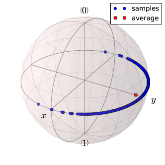
(a)

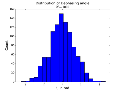
(b)

Figure 1: LABEL:sub@fig:dephasing:a Randomly sampled dephasing operations drawn from the Von Mises distribution as described above and applied to the Bloch vector $[0,1,0]^{\top}$. LABEL:sub@fig:dephasing:b Histogram of random samples of dephasing angle $\theta$ sampled according to the Von Mises distribution corresponding to the data in LABEL:sub@fig:dephasing:a.

IV.2 Depolarizing noise

The Choi matrix for Pauli channel depolarizing noise is $(1-p_{x}-p_{y}-p_{z})|\sigma_{I}\rangle\rangle\langle\langle\sigma_{I}|+p_{x}|\sigma_{X}\rangle\rangle\langle\langle\sigma_{X}|+p_{y}|\sigma_{Y}\rangle\rangle\langle\langle\sigma_{Y}|+p_{z}|\sigma_{Z}\rangle\rangle\langle\langle\sigma_{Z}|$, with $p_{i}\in[0,1]$, $\sum p_{i}\leq 1$. Converting this to a Pauli transfer matrix yields

$$\mathcal{R} =(1-p_{x}-p_{y}-p_{z})I_{4}$$ (25)

$$+p_{x}\begin{bmatrix}1&0&0&0\\ 0&1&0&0\\ 0&0&-1&0\\ 0&0&0&-1\end{bmatrix}+p_{y}\begin{bmatrix}1&0&0&0\\ 0&-1&0&0\\ 0&0&1&0\\ 0&0&0&-1\end{bmatrix}+p_{z}\begin{bmatrix}1&0&0&0\\ 0&-1&0&0\\ 0&0&-1&0\\ 0&0&0&1\end{bmatrix}$$

so the corresponding affine form is

$$\varphi\to\underbrace{\begin{bmatrix}1-2(p_{y}+p_{z})&0&0\\ 0&1-2(p_{x}+p_{z})&0\\ 0&0&1-2(p_{x}+p_{y})\end{bmatrix}}_{A_{p}}\varphi+\begin{bmatrix}0\\ 0\\ 0\end{bmatrix}\,.$$ (26)

Note that this is consistent with (22) under the assumption that $\zeta(t)$ in (18) is zero mean so that $E[\operatorname{Im}\alpha^{2}]=0$. If we treat the contraction matrix $A_{p}$ in (26) as an average of random elements in $SO(3)$, we can apply the matrix-Fisher distribution on $SO(3)$. Figure 2 shows random samples of depolarizing channels drawn from the matrix-Fisher distribution on $SO(3)$ whose average corresponds to $p_{x}=0.001$, $p_{y}=0.01$ and $p_{z}=0.1$.

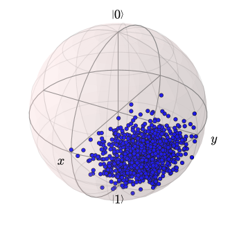
Figure 2: Randomly generated unitary maps whose average is the depolarizing channel with $p_{x}=0.001$, $p_{y}=0.01$, and $p_{z}=0.1$ sampled according to the Von Mises-Fisher distribution on $SO(3)$ applied to Bloch vector $[\frac{\sqrt{2}}{2},\frac{\sqrt{2}}{2},0]^{\top}$.

Since the depolarizing channel is expressed as a mixture over unitary maps, it is natural to treat a depolarizing channel as the average of random unitary operations as in Figure 2. However, the same depolarizing channel in Choi form could serve as the sufficient statistic for a frame-Bingham distribution as described in Section III.2. In this case, the random CPTP maps generated would be non-unitary with probability 1. Figure 3a shows random samples generated from the frame-Bingham distribution applied to the same input state as Figure 2. Note that the shapes of the output distributions are are distinctly different. Furthermore, although it cannot be seen from the figures themselves, since the operations in Figure 2 are unitary, the output states are all on the surface of the Bloch sphere. However, in the case of the frame-Bingham distribution, the states are pulled in to the Bloch sphere, resulting in a distribution of norms of Bloch vectors as in Figure 3b.

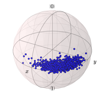
(a)

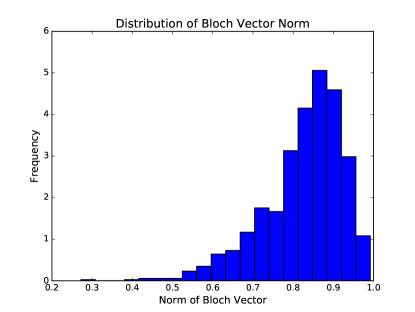
(b)

Figure 3: LABEL:sub@fig:depol2:a Randomly generated CPTP maps whose average is the depolarizing channel with $p_{x}=0.001$, $p_{y}=0.01$, and $p_{z}=0.1$ sampled according to the frame-Bingham distribution applied to Bloch vector $[\frac{\sqrt{2}}{2},\frac{\sqrt{2}}{2},0]^{\top}$. LABEL:sub@fig:depol2:b Histogram of norms of output Bloch vectors corresponding to the data in LABEL:sub@fig:depol2:a.

IV.3 Amplitude Damping

An example amplitude damping channel Nielsen and Chuang (2010), parameterized by $\gamma$ is defined by Kraus operators

$$A_{1} =\begin{bmatrix}1&0\\ 0&\sqrt{1-\gamma}\end{bmatrix}\,, A_{2} =\begin{bmatrix}0&\sqrt{\gamma}\\ 0&0\end{bmatrix}\,.$$ (27)

The corresponding PTM is

$$\mathcal{R}=\begin{bmatrix}1&0&0&0\\ 0&\sqrt{1-\gamma}&0&0\\ 0&0&\sqrt{1-\gamma}&0\\ \gamma&0&0&1-\gamma\end{bmatrix}$$ (28)

which the first column indicates is non-unital, meaning the techniques in Section III.1 do not apply. Furthermore, amplitude damping belongs to a class of CPTP maps that cannot be generated as the average of a random (i.e., non-constant) CPTP map, as discussed in Section V. That said, we can generate distributions whose average is nearly the amplitude damping channel by using the Stiefel representation

$$\mathcal{S}=\begin{bmatrix}1&0\\ 0&\sqrt{1-\gamma}\\ 0&\sqrt{\gamma}\\ 0&0\\ 0&0\\ 0&0\\ 0&0\\ 0&0\\ \end{bmatrix}\,,$$ (29)

and set $(1-\varepsilon)\mathcal{S}$ (for small $\varepsilon$) as the average value for complex matrix-Fisher distribution as described in Section III.2. Figure 4 shows the action of randomly sampled approximate amplitude damping channels ($\gamma=0.01$) on the initial state $|0\rangle$, for decreasing $\varepsilon$. For reference, we find empirically that for $\varepsilon=0.001$ the diamond norm error between the average approximate amplitude damping channel and the actual is around $0.05$.

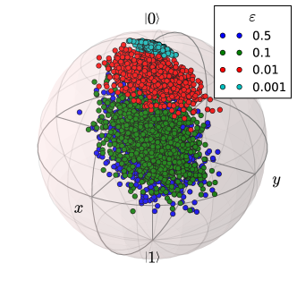
Figure 4: Attempts to approximate an amplitude damping channel ($\gamma=0.01)$ using the matrix-Fisher distribution on the Stiefel representation for varying $\varepsilon$. Random samples are applied to the state $|0\rangle$ for presentation.

In addition to the matrix-Fisher approach, we can also use the frame-Bingham distribution to attempt to approximate the amplitude damping channel using the corresponding Choi matrix

$$\Lambda_{\gamma}=\begin{bmatrix}1&0&0&\sqrt{1-\gamma}\\ 0&0&0&0\\ 0&0&\gamma&0\\ \sqrt{1-\gamma}&0&0&1-\gamma\end{bmatrix}\,\,.$$ (30)

The first caveat to note is that the Choi matrix for an amplitude damping channel is in some sense singular, since it indicates that $\xi_{2}$ in the the alternative stiefel representation $\xi$ is always 0. This singularity is easily handled by a slight modification to the projection step in Hoff (2009) for the first column of $\xi$. Even with this additional step, the frame-Bingham distribution is still not capable of averaging to an amplitude damping channel. Instead, estimating the parameters in an attempt match the diagonal terms of the Choi matrix with a frame-Bingham distribution, while trying to concentrate the distribution as strongly as possible is shown in Figure 5a.

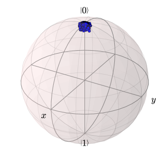
(a)

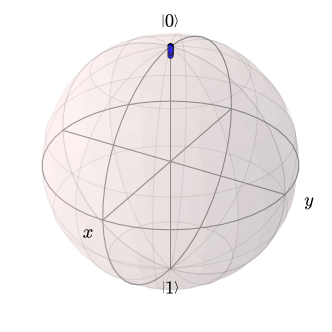
(b)

Figure 5: LABEL:sub@fig:depol2:a Randomly generated CPTP maps whose average is the depolarizing channel with $p_{x}=0.001$, $p_{y}=0.01$, and $p_{z}=0.1$ sampled according to the frame-Bingham distribution applied to Bloch vector $[\frac{\sqrt{2}}{2},\frac{\sqrt{2}}{2},0]^{\top}$. LABEL:sub@fig:depol2:b Histogram of norms of output Bloch vectors corresponding to the data in LABEL:sub@fig:depol2:a.

An alternative approximation that also uses the frame-Bingham distribution is to further restrict the distribution generated in the projection step to be a random amplitude damping channel. Again, the average of random amplitude damping channels will not be an amplitude damping channel, but we attempt to approximate by matching the diagonal terms of the Choi matrix. This approach is shown in Figure 5b. In this case, since every operation produced is an amplitude damping channel for some random $\gamma$, the map of the state $|0\rangle$ lies on the axis, unlike the other approximation cases.

IV.4 A Non-Unital Example

Consider the amplitude damping channel above followed by the depolarizing channel. In PTM form, this channel is

$$\mathcal{R}=\begin{bmatrix}1&0&0&0\\ 0&(1-2(p_{y}+p_{z}))\sqrt{(}1-\gamma)&0&0\\ 0&0&(1-2(p_{x}+p_{z}))\sqrt{(}1-\gamma)&0\\ (1-2(p_{x}+p_{y}))\gamma&0&0&(1-2(p_{x}+p_{y}))(1-\gamma)\\ \end{bmatrix}$$ (31)

which is non-unital, but unlike the pure amplitude damping channel, it can be represented by a frame-Bingham distribution as shown in Figure 6.

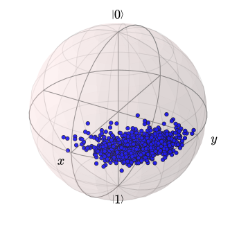
(a)

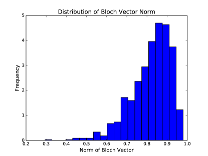
(b)

Figure 6: LABEL:sub@fig:depol2:a Randomly generated CPTP maps whose average is the nonunital channel in (31) with $\gamma=0.01$, $p_{x}=0.001$, $p_{y}=0.01$, and $p_{z}=0.1$ sampled according to the frame-Bingham distribution applied to Bloch vector $[\frac{\sqrt{2}}{2},\frac{\sqrt{2}}{2},0]^{\top}$. LABEL:sub@fig:depol2:b Histogram of norms of output Bloch vectors corresponding to the data in LABEL:sub@fig:nonunital:a.

V CPTP Maps Representable as Random CPTP Maps

In this section we will give a geometric characterization the set of CPTP maps (of a given size) which can be represented by the average of a random CPTP map of the same size. Note that this applies to any method of generating random CPTP maps beyond what is presented here, including Pauli-channel error models and stochastic master equation approaches. For a convex set $\mathcal{C}$, a point $x\in\mathcal{C}$ is said to be an extreme point if $\mathcal{C}\setminus\{x\}$ is still a convex set. This definition implies that an extreme point cannot be represented as the convex combination of other points in $\mathcal{C}$, and as such an extreme point $x$ cannot be the average of a non-trivial random variable taking elements in $\mathcal{C}$. Note that there is a distinction between extreme points and boundary points of $\mathcal{C}$, all extreme points are boundary points, but not all boundary points are extreme (consider the edges of a square, for example). Points that are not extreme points must be equal to some convex combination of extreme points, and thus can be trivially represented as the average over these points when the extreme points are sampled according to their weight in the convex combination. Thus, the question of representability in this manner is an exercise in classifying the extreme points of the space of CPTP maps.

For general $N$, this appears to be an open question, however for the case where $N=2$, the convex geometry of CPTP maps has been completely characterized in Ruskai et al. (2002). In particular they show

Theorem V.1 (Theorem 13 in Ruskai et al. (2002)).

If a CPTP map written in Kraus form $\{A_{k}\}$ requires exactly two Kraus operators, then it is either unital or an extreme point.

Since the amplitude damping channel requires two Kraus operators and is non-unital, it must be an extreme point. Thus, it cannot serve as the average for any non-trivial random CPTP map operating on $N\times N$ density operators, and as such we were unable to exactly reproduce the amplitude damping channel in Section IV.3. Furthermore, any random CP map on $N\times N$ density operators that has an amplitude damping channel as its average, must take values that are not TP with non-zero probability (c.f. Burgarth et al. (2016)).

VI Conclusion

In this manuscript, we have presented a number of connections between distributions studied in directional and orientation statistics to various representations of quantum states and quantum operations. Furthermore, by connecting the notion of an average quantum state or operation to a sufficient statistic of an exponential family we are able to define the unique probability distribution that maximizes entropy while still satisfying the target average.

From a modeling and simulation perspective, we foresee a number of applications of this work to the study of quantum systems. The generation of random quantum states and operations with a specified average that can be sampled in an absolutely continuous manner (as compared to the standard Pauli error channel) can have a drastic effect on simulation results for e.g., error correction and threshold computations Barnes et al. . Additionally, this sort of statistical foundation allows for the exploration of correlated quantum errors which will be present in a non-Markovian environment.

From an inference and analytic perspective, we expect that the statistical models presented here will be useful for developing statistical tests and analysis. For example, tests for correlation from orientation statistics could be adapted to provide tests and measures for non-Markovianity in quantum channels. One can also envision adapting concepts such as graphical models from applied statistics and machine learning to complex inference problems of relevance to quantum information, such as tomography.

The work here also touches on some interesting questions on the geometry of quantum operations, for example, further investigation is warranted of the exact connection between the vastly different geometries of the Stiefel representation (a differential geometry on a surface) and the convex geometry of Choi matrices. Such a viewpoint may be useful in characterizing extreme points in the convex geometry of quantum operations. Additionally, there may be interesting connections between the information geometry of the exponential families presented here and traditional concepts from quantum information. For example, does the Kullback-Leibler divergence between elements of the exponential family relate to any known distance measure between quantum operations or are there alternative information geometries which maximize expected diamond norm?