The effects of external planets on inner systems: multiplicities, inclinations, and pathways to eccentric warm Jupiters

Abstract

We study how close-in systems such as those detected by Kepler are affected by the dynamics of bodies in the outer system. We consider two scenarios: outer systems of giant planets potentially unstable to planet–planet scattering, and wide binaries that may be capable of driving Kozai or other secular variations of outer planets’ eccentricities. Dynamical excitation of planets in the outer system reduces the multiplicity of Kepler-detectable planets in the inner system in $\sim 20-25\%$ of our systems. Accounting for the occurrence rates of wide-orbit planets and binary stars, $\approx 18\%$ of close-in systems could be destabilised by their outer companions in this way. This provides some contribution to the apparent excess of systems with a single transiting planet compared to multiple; however, it only contributes at most 25% of the excess. The effects of the outer dynamics can generate systems similar to Kepler-56 (two coplanar planets significantly misaligned with the host star) and Kepler-108 (two significantly non-coplanar planets in a binary). We also identify three pathways to the formation of eccentric warm Jupiters resulting from the interaction between outer and inner systems: direct inelastic collision between an eccentric outer and an inner planet; secular eccentricity oscillations that may “freeze out” when scattering resolves in the outer system; and scattering in the inner system followed by “uplift”, where inner planets are removed by interaction with the outer planets. In these scenarios, the formation of eccentric warm Jupiters is a signature of a past history of violent dynamics among massive planets beyond $\sim 1$ au.

1 Introduction

The population of planet candidates detected by Kepler shows a surplus of systems showing only one transiting planet (Johansen et al., 2012; Ballard & Johnson, 2016), a finding that has been dubbed the “Kepler Dichotomy”. This translates into an excess of systems with only one planet in the region probed by Kepler, as altering the distribution of mutual inclinations amongst triple-planet systems cannot simultaneously account for the numbers of single-, double- and triple-transit systems (Johansen et al., 2012): a large fraction of the double-transit systems could be produced by intrinsically triple-planet systems, but this still requires an additional population of intrinsically single-planet systems to match the large observed number of single-transit systems. This suggests that Nature produces two distinct populations of inner planetary systems: one population of intrinsically single planets, and an additional population of multiple systems whose multiplicity peaks at three planets or higher. There are three possible explanations for this excess:

• There is a high false positive rate amongst single-transit systems. While most Kepler multiple systems appear to be genuine (Rowe et al., 2014), Santerne et al. (2016) find a $\sim 50\%$ false-positive rate for single giant Kepler candidates. They speculate that the absolute number of false positives may be higher for the smaller candidates, although the rate could fall due to the increased frequency of smaller planets.

• Many systems form only one planet within $\lesssim 1$ au, while a smaller number form multiple. Coleman & Nelson (2016) find that, when starting from a large number of embryos, systems resembling the Kepler singles only arise if one planet grows to be massive enough to clear out its neighbours, and speculate that many systems must form small numbers of embryos. Unfortunately, predicting the formation times, locations and numbers of these embryos is challenging, despite the significant effects that these initial conditions have on the embryos’ subsequent growth and migration (e.g., Bitsch et al., 2015).

• Many systems form multiple planets within $\lesssim 1$ au, but many are later reduced in multiplicity by subsequent dynamical evolution as planets collide. This route may be supported by an additional “dichotomy” in the distributions of orbital eccentricities (see Shabram et al., 2016, who argue for a two-component model for the eccentricity distribution, with a low-$e$ ($\sim 0.01$) and a high-$e$ ($\sim 0.2$) component; Xie et al. 2016 argue for a similar “eccentricity dichotomy”) and stellar obliquities (Morton & Winn 2014 find that stars with a single transiting planet have higher obliquity than those with multiple planets, while Campante et al. 2016 favour a mixture model for the obliquities of single-planet host stars but a single model for hosts of multiple planets). This evolution may be driven by the internal dynamics of the Kepler multiples (e.g., Johansen et al., 2012; Pu & Wu, 2015; Volk & Gladman, 2015) or by the effects of outer bodies such as binary stars or outer giant planets on the inner system (e.g., Mustill et al., 2015).

In this paper, we further explore the effects a dynamically active outer system can have on systems of multiple inner planets. We build on our previous work (Mustill et al., 2015), in which we considered the effects of a planet with an arbitrarily-imposed eccentricity on an inner system, by consistently modelling the dynamics in the outer system leading to such eccentricity excitation, through Kozai cycles or planet–planet scattering. We gauge the contribution of disruptive outer bodies to the Kepler multiplicity function by destabilising and inclining inner systems, show that it is possible to occasionally generate large mutual inclinations or obliquities as in the tilted two-planet system Kepler-56 (Huber et al., 2013) and the mutually inclined Kepler-108 (Mills & Fabrycky, 2016), and identify several routes to forming eccentric warm Jupiters at a few tenths of an au.

Can the Kepler Dichotomy be resolved by appealing to instabilities driven by the internal dynamics of inner systems (henceforth, anything with an orbital period $P<240$ d)? Probably not entirely: Kepler triple-planet systems, for example, are robust to internal dynamical evolution. Johansen et al. (2012) showed that these triple-planet systems are too widely separated to undergo instability unless their masses are increased unrealistically, by a factor of around 100. Furthermore, when forced into instability in this way the outcome is typically only a reduction to a two-planet system. However, Pu & Wu (2015) show that the higher-multiplicity systems are less stable, consistent with being the survivors from a continuous primordial population where the more closely-spaced systems were unstable. Meanwhile, Becker & Adams (2016) find that Kepler multi-planet systems are inefficient at self-exciting their mutual inclinations: flat systems remain flat, and retain their high probablility of multiple transits.

A high occurrence rate of inner planetary systems ($\sim 50\%$) has been revealed by both RV surveys (Mayor et al., 2011) and Kepler (Fressin et al., 2013). But many of these inner systems do not exist in isolation. They may have wide-orbit companion planets, as in the case of Kepler-167, which possesses three super-Earths within 0.15 au together with a transiting giant planet at 1.9 au (Kipping et al., 2016). A number of studies have found wide-orbit candidates in the Kepler light curves which transit only a small number of times and therefore are excluded from the KOI listings (Wang et al., 2015; Osborn et al., 2016); Uehara et al. (2016) estimate that at least 20% of compact multi-planet systems also host giant planets beyond 3 au, based on single-transit events in the KOIs; and Foreman-Mackey et al. (2016) estimate an average of 2 planets per star with periods between 2 and 25 years and radii between $0.1$ and $1\mathrm{\,R_{J}}$, $0.4$ planets per star in the same period range with radii between $0.4$ and $1\mathrm{\,R_{J}}$, and that these wide-orbit planets occur disproportionately often around stars already hosting inner planet candidates. Knutson et al. (2014) find that $50\%$ of hot Jupiter hosts also have a giant planet companion between 1 and 20 au, while Bryan et al. (2016) similarly find an occurrence rate of $50\%$ for outer planetary companions to RV-detected inner planets of a range of masses, although their sample is more metal-rich than the Kepler targets. Wang et al. (2015) found that half of their long-period Kepler candidates exhibited transit timing variations, suggesting multiplicity.

Regarding the presence of planetary systems in wide binaries, some Kepler systems, such as Kepler-444 (Campante et al., 2015) and Kepler-108 (Mills & Fabrycky, 2016), reside in wide binaries. Ngo et al. (2015, 2016) estimate that $50\%$ of hot Jupiters have a stellar companion between 50 and 2 000 au, around twice the rate for the average field star. There is currently debate about the extent to which the presence of an outer binary companion affects the existence of inner Kepler planets (e.g., Wang et al., 2014; Deacon et al., 2016; Kraus et al., 2016).

Statistics from systems without detected inner planets also reveal the prevalence of outer bodies. RV surveys reveal a population of “Jupiter analogues” (variously defined as low-eccentricity $\sim$Jupiter-mass planets at several au) of a few percent (Rowan et al., 2016; Wittenmyer et al., 2016). Direct imaging surveys are sensitive to super-Jovian planets at tens of au, finding an occurrence rate of around $10\%$ (Vigan et al., 2012) for stars more massive than the Sun, falling to $1-2\%$ for Solar-type stars (Galicher et al., 2016). Microlensing reveals an occurrence rate of $\sim 50\%$ for ice-line planets more massive than Neptune, where the host stars were typically sub-Solar in mass (Shvartzvald et al., 2016). Around half of Sun-like stars are in members of multiple stellar systems, with a period distribution peaking at $\sim 10^{5}$ days (Raghavan et al., 2010; Duchêne & Kraus, 2013). Compared to the statistics in the previous paragraph, it may be that stars with known inner planets are more likely than other stars to host wide-orbit giant planets, although one should be wary of biases such as for example in the stellar metallicities.

The configuration and evolution of bodies in the outer system can have significant dynamical effects on these inner systems. In Mustill et al. (2015), we showed that a high-eccentricity giant planet en route to becoming a hot Jupiter will destroy any existing close-in planets, thus explaining why hot Jupiters are typically not seen with close, low-mass companions. Mustill et al. (2015) also showed that, as the orbital binding energy of the eccentric giant can be comparable to that of the inner planets, the giant can in fact be ejected as a result of the interactions with the inner system, which may itself be reduced in multiplicity. Although hot Jupiters are relatively rare, being found around only $\sim 1\%$ of stars (Mayor et al., 2011; Howard et al., 2012; Fressin et al., 2013; Santerne et al., 2016), models of high-eccentricity migration of hot Jupiters typically find that many more migrating giants are tidally disrupted than go on to become hot Jupiters (e.g., Petrovich, 2015; Anderson et al., 2016; Muñoz et al., 2016; Petrovich & Tremaine, 2016). Lower-mass planets may well be injected into the inner systems by the same dynamical mechanisms—scattering and Kozai perturbations—that give rise to hot Jupiters, and many outer planets thus sent inwards will attain pericentres insufficiently small for tidal circularisation, yet small enough to interact with inner planets at a few tenths of an au. All this motivates a general investigation into the influence of outer systems on inner Kepler-detectable planets.

While the bulk of Kepler-detected planets lie at a few tenths of an au, work has shown that instabilities in outer systems can be devastating for material in the habitable zone at $\sim 1$ au (Veras & Armitage, 2005, 2006; Raymond et al., 2011, 2012; Matsumura et al., 2013; Kaib & Chambers, 2016). Carrera et al. (2016) find that the survivability of bodies increases closer to the star, and (Huang et al., 2016a) study the effects on the excitation of Kepler-like super Earths. Direct scattering is the most obvious effect of eccentricity enhancement in the outer system, but secular resonances can also play a role in destabilising inner systems (Matsumura et al., 2013; Carrera et al., 2016). Secular interactions can also have more subtle effects on inner systems, resulting in gentle tilts (Gratia & Fabrycky, 2017), or excitation of mutual inclination (Hansen, 2016; Lai & Pu, 2016), which in turn can contribute to the observed multiplicities seen by Kepler.

Dynamical interaction between inner and outer systems may also account for the existence of eccentric warm Jupiters: giant planets with semi-major axes of a few tenths of an au and eccentricities of order $0.5$. While planet–planet scattering has long been recognised as a source of eccentricity excitation of giant planets (e.g. Rasio & Ford, 1996; Weidenschilling & Marzari, 1996; Chatterjee et al., 2008; Jurić & Tremaine, 2008; Raymond et al., 2011; Kaib et al., 2013), Petrovich et al. (2014) showed that this process is ineffective at exciting eccentricities close to the star: on tight orbits, planets have a higher Keplerian velocity and so in order to impart a given change in velocity, a close encounter must occur at a smaller separation due to the reduced gravitational focusing, and such close encounters result instead in physical collision. Nor can eccentric warm Jupiters be explained by “fast” tidal migration of giant planets en route to forming hot Jupiters, as the eccentricities of the observed planets lie below the tidal circularisation tracks along which such planets would migrate. Possible explanations are “slow” tidal migration, in which tidal dissipation only occurs briefly at the tip of a secular eccentricity cycle (Dawson & Chiang, 2014; Dong et al., 2014; Petrovich, 2015; Petrovich & Tremaine, 2016), and the physical collision of eccentric migrating giant planets with other planets on close-in orbits (Mustill et al., 2015). In this paper, we describe several other routes to the formation of eccentric warm Jupiters.

In summary, at least a few 10s of per cent of inner systems can be expected to host outer planets and/or stars. In this paper we study the effects of these outer bodies on inner systems with $N$-body integrations. We set up two scenarios: outer planets in binary systems that may be subject to Lidov–Kozai oscillations (Lidov, 1962; Kozai, 1962; Naoz, 2016), and tightly-packed systems of outer planets that are unstable to scattering; Jurić & Tremaine (2008) and Raymond et al. (2011) show that the eccentricity distribution of giant planets is consistent with around $75-83\%$ of them having originally come from unstable multiple systems. We investigate the effects that the dynamics of the outer system have on the multiplicities of the inner planets and on their mutual inclinations. In Section 2 we describe the set-up of our $N$-body integrations. We describe the outcomes of a set of control integrations in Section 3. We give the results for planets in binary systems in Section 4 and for unstable scattering systems in Section 5, describing the effects on the multiplicities and mutual inclinations of inner planetary systems. In Section 6 we describe three mechanisms leading to the formation of eccentric warm Jupiters: collision between an inner and an eccentric outer planet (Section 6.1), secular forcing aided by “freeze-out” (Section 6.2), and in-situ scattering aided by “uplift” from the outer system (Section 6.3). We discuss our results in Section 7, notably the effects on Kepler systems’ multiplicities (Section 7.2.1) and mutual inclinations (Section 7.2.2), the generation of large obliquities or mutual inclinations (Section 7.3), and summarise in Section 8.

2 Numerical methods and setup

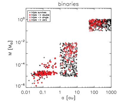
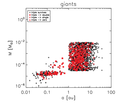
Figure 1: Initial semi-major axes and masses of all bodies in our Binaries and Giants simulations. There are three inner planets per system; inner planets are drawn from triple-planet KOI systems. In Binaries there is one additional outer planet and one stellar companion per system, while in Giants there are four outer planets. Bodies are colour-coded according to whether or not their system was unstable (defined as the loss of one or more of the inner triple). 88/400 of the Binaries simulations, and 99/400 of the Giants simulations, resulted in destabilisation of the inner system.

We conduct our $N$-body integrations with the Bulirsch–Stoer integrator of the Mercury integrator package (Chambers, 1999). The tolerance parameter is set to $10^{-13}$. Simulations are run for 10 Myr. We incorporate leading-order post-Newtonian terms into the integrator: these are essential particularly for the binary systems to ensure that single-planet survivors correctly have their Kozai cycles suppressed, as a single planet in an inclined binary system will be protected from Kozai cycles by the relativistic precession (e.g. Ford et al., 2000; Fabrycky & Tremaine, 2007). In this paper we treat collisions as perfect mergers; we intend to explore the effects of different collision prescriptions in a future paper. Bodies that pass within one stellar radius of the centre of the star are assumed to undergo an inelastic collision with this object; in reality, some may undergo tidal circularisation to become planets on tight circular orbits such as hot Jupiters.

Our systems are constructed from a combination of actual Kepler Objects of Interest (KOIs) for the inner system and artificial planets and stellar companions for the outer system. For most integration sets we choose triple-planet KOI systems from the Q1–Q17 Kepler DR24 for the inner planets (Coughlin et al., 2016). KOIs are subjected to the same cuts as in Lissauer et al. (2011) and Johansen et al. (2012), and in addition KOIs labelled as false positives in the NASA exoplanet archive are removed. KOIs in candidate triple-planet systems were then assigned masses acording to the deterministic mass–radius relation of Weiss & Marcy (2014). The probability of seeing each system as a triple-planet KOI system was calculated assuming an inclination distribution with $\beta=5^{\circ}$ (see Fig 3 of Johansen et al., 2012, for this distribution). When building a population of systems for the simulations described below, KOI systems were drawn weighted by the inverse of the probability of seeing them as a triple-transiting system, thus generating a model population closer to the actual debiased population of multiple systems.

Our simulations are divided into three main classes. First we integrate a Control set of the triple KOI systems in isolation. Systems which are stable are then used as templates for two sets of simulations with outer perturbers: Binaries, with binary stellar companions and outer planetary companions, and Giants, with outer planetary companions. The Binaries and Giants classes are themselves subdivided into several sets.

We refer the reader to Section 7.5 for a detailed discussion of our initial conditions. Here we note that our outer systems are motivated by current observational constraints on the occurrence rates and distributions of masses and semimajor axes of wide-orbit planets and binary stars, but that we assume that there is no correlation between the formation of the inner and the outer planets.

2.1 The Control class

We first evolve the triple-planet candidate KOI systems in isolation. They were then cloned 8 times with zero eccentricities, inclinations assigned with $\beta=5^{\circ}$, and randomised orbital phases, and integrated for 1 Myr. Systems where one or more clones experienced close encounters between the planets were removed from further consideration (see Section 3 below). We identified one such unstable system (KOI00284). We also removed one system that lies very close to a 4:2:1 mean motion commensurability (KOI01426). The remaining 86 systems were used as templates for the inner triple-planet systems for the main integration sets described below.

2.2 The Binaries class

The Binaries class is divided into the Binaries simulation set proper, Binaries-flat, and Binaries-0pl.

For our simulation set Binaries we add one extra planet and one wide binary companion. The planet has a mass ranging from $3-3000\mathrm{\,M}_{\oplus}$ drawn from a uniform distribution in log space, a semi-major axis ranging from $1-10$ au drawn uniformly in log space, zero eccentricity, and an inclination assigned the same way as the inner planets’. The binary has a mass drawn uniformly from $0.1\mathrm{\,M}_{\odot}$ to the primary’s mass, an eccentricity drawn uniformly between 0 and 1, an inclination drawn from an isotropic distribution and a period drawn form a lognormal distribution with a peak at $10^{5}$ days and a standard deviation of 2.3 dex. Binaries with semi-major axes smaller than 50 or greater than 1000 au were then resampled. See Duchêne & Kraus (2013) for the justification for our binary population. A misalignment for the orbital inclinations of these binaries is consistent with observations of discs in young binary systems (Jensen & Akeson, 2014; Brinch et al., 2016) and expected from simulations of star formation (Bate, 2012). The planet properties are harder to justify as the region beyond 1 au is subject to selection biases. However, the mass and semi-major axis distributions of giant planets are approximately flat in log space (e.g., Cumming et al., 2008). The initial semi-major axes and masses of all bodies in our Binaries simulations are shown in Figure 1.

The Binaries-flat set is set up similarly to the Binaries set itself, save for the inclinations of the four planets, which are all set to $0^{\circ}$. The wide binary companion retains its isotropic distribution. The Binaries-0pl set is set up similarly to the Binaries set, except that there is no extra planet added: the systems comprise the triple KOIs and a wide binary. This is to verify that the effects of the wide binary star acting alone on the KOI systems are negligible. Finally, Binaries2 uses the same outer systems (binary star plus extra planet) as the Binaries set, but the inner planetary systems are taken from double-planet, not triple-planet, observed KOI systems.

2.3 The Giants class

As with the Binaries class, we divide Giants into Giants proper, Giants-flat and Giants-1pl.

For our simulation set Giants we add four extra planets. Masses are drawn uniformly in log space from $10-3000\mathrm{M}_{\oplus}$, eccentricities are zero, and inclinations assigned with $\beta=5^{\circ}$. The semi-major axis of the inner planet is drawn randomly in log space from $1-3$ au, while subsequent planets are placed $4-6$ mutual Hill radii beyond this. This places the systems on the edge of stability and ensures that many systems will experience instability during the 10Myr integration time. Jurić & Tremaine (2008) and Raymond et al. (2011) argue that the eccentricity distribution of giant planets is best reproduced if the majority of such planets come from unstable multiple systems that undergo scattering to excite planetary eccentricities. The initial semi-major axes and masses of all bodies in the Giants set are shown in the right-hand panel of Figure 1. We further discuss the initial conditions for our simulations in Section 7.5.

To complement Giants, we also run a Giants-flat set, with similar initial conditions but with inclinations of all planets reduced to $\beta=0.1^{\circ}$ (unlike in Binaries-flat we avoid exact coplanarity of the inner planets, as these have no intrinsic way to break the symmetry of exact coplanarity, a role filled by the inclined binary in Binaries-flat). Giants2 has its outer planets initialised in the same way as Giants, but the inner triple-planet KOI systems are replaced by double-planet KOI systems as in Binaries2. We also run a Giants-1pl set, where only the first of the four outer giants is placed. This is to verify that a single unexcited outer planet does not significantly afect the inner system.

3 The control sample

As described in Section 2.1, we first integrated the Kepler triple-planet systems in isolation. Each system was cloned 8 times, assigned different orbital inclinations and phases, and integrated for 1 Myr. We identified one unstable system: KOI00284 (alias Kepler-132), which has planets at 6.18 and 6.41 days’ period. This system was also identified as possessing a binary companion by Lissauer et al. (2014), who inferred that not all of the planets orbit the same star.

The majority of these isolated systems experienced very little eccentricity excitation, with the median of the maximum eccentricity attained over 1 Myr being $3.6\times 10^{-4}$, and only $1.6\%$ of planets ever attaining $e>0.01$. The most excited system was KOI01426 (alias Kepler-297), in which one planet always attained a maximum eccentricity of $\approx 0.07$. This system lies close to a 4:2:1 period commensurability, and we removed this system in case the resonant dynamics would be important for its stabilisation.

The stability of the vast majority of these Kepler triple-planet systems agrees with previous analyses (Johansen et al., 2012; Fabrycky et al., 2014). The two systems identified above (KOI00284 and KOI01426) were discarded when setting up the inner systems for the main integration sets.

4 Population synthesis I: Binaries

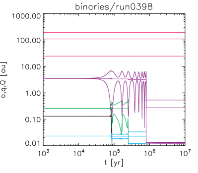
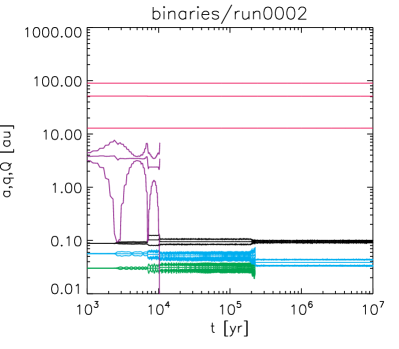
Figure 2: Example evolution of Binaries integrations, showing semi-major axes, pericentres and apocentres of all bodies in a system. The binary companion is in magenta, the outer planet in purple, and the Kepler triple-planet system in blue, green and black. Left: A giant planet is forced by Kozai cycles into the inner system, clearing out the inner planets. This planet ends with a pericentre $\sim 0.01$ au, and would in time circularise to form a hot Jupiter. Right: Here the outer planet is swiftly forced into the star, but triggers a delayed instability causing a reduction in inner system multiplicity 200 kyr later.

In our Binaries simulation set we integrate 400 systems. Example evolution is shown in the Figure 2. In the left panel, a $0.6$ Jupiter-mass planet is sent into the inner system where it forces two super-Earths into the star, before colliding with the third. This inelastic collision drains specific orbital energy from the giant, leaving it as a highly-eccentric warm Jupiter with a pericentre of $\sim 0.01$ au whose Kozai oscillations have been shut off by relativistic precession. This planet would, in time, tidally circularise to form a hot Jupiter with no companions in the inner system. In the right panel, the outer giant is forced into the star by Kozai perturbations, but during each high-eccentricity phase it excites the eccentricities of the inner planets. This triggers a delayed instability about $0.2$ Myr later, causing a merger of the two inner planets. The mutual inclination of the survivors is moderately excited, around $11^{\circ}$.

4.1 Effects on outer system

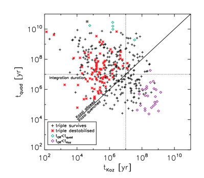
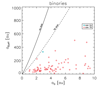
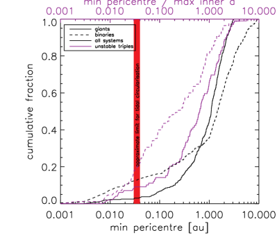
Figure 3: Prospects for the formation of Hot Jupiters in our integrations. Top left: Competition between Kozai forcing from the binary and secular perturbations from the inner three planets for all outer planets in the Binaries simulations. The “effective” semimajor axis of the binary ($a_{\mathrm{B,eff}}=a_{\mathrm{B}}\sqrt{1-e_{\mathrm{B}}^{2}}$) is plotted against the outer giant planet’s semimajor axis $a_{\mathrm{G}}$. The inner system imposes an upper limit to the outer planet’s eccentricity (see Eq 6); systems where this eccentricity is sufficient to allow the outer planet’s pericentre $q_{\mathrm{G}}$ to become smaller than the outermost inner planet’s semimajor axis $a_{\mathrm{in}}$ are shown in purple (actual initial inclinations in the simulations) and red (an initial inclination of $90^{\circ}$, the most effective case). This gives an estimate of 62/400 systems possessing outer planets whose pericentres can be driven to overlap the inner planets’ orbits. Top right: Timescales for precession of the outer planet in the Binaries systems induced by the outer companion ($t_{\mathrm{Koz}}$) and by the inner planets ($t_{\mathrm{quad}}$; quadrupole approximation). Kozai cycles are quenched if $t_{\mathrm{quad}}\lesssim t_{\mathrm{Koz}}$. Red and black points show whether the inner planets in a system were destabilised: this can only happen if $t_{\mathrm{quad}}>t_{\mathrm{Koz}}$ so that the Kozai mechanism can excite the giant planet’s eccentricity. We also show as diamonds systems where the precession timescale of the outer planet due to general relativity is less than the Kozai timescale (purple points towards the right) or the quadrupole precession from the inner system (green points towards the top). For the former systems, GR precession would quench the Kozai effect even in the absence of the inner system, while for the latter systems, the GR precession dominates over that from the planetary quadrupole. Bottom left: Allowed parameter space for hot Jupiter formation for outer planets in the Binaries systems with $m>M_{\mathrm{Saturn}}$ based on our initial conditions. We show only systems where the inner planets were destabilised. Turquoise stars represent planets that can be tidally circularised to form hot Jupiters; red diamonds represent planets that can be tidally disrupted at the Roche limit. The solid and dashed lines represent the limits for fiducial $m_{\mathrm{pl}}=M_{\mathrm{Jupiter}}$ and $m_{\mathrm{B}}=M_{\odot}$. Bottom right: Minimum pericentres attained over the course of the integration by the outer planet in the Binaries and Giants simulations. Around 10–15% in Binaries attain either a sufficiently small pericentre to begin tidal circularistion of the orbit, and/or collide with the star, a figure comparable to studies of hot Jupiter migration by Kozai cycles and tidal friction. The Giants simulations are much less efficient at generating small pericentres. In purple the minimum pericentre is shown as a fraction of the semimajor axis of the outermost inner planet (upper $x$-axis), for systems where the inner triple was destabilised. In most of these systems the orbit of an outer planet overlaps with those of the inner planets, but there is a minority of systems where destabilisation occurs at a distance.

Eccentricity forcing by Kozai cycles followed by dissipation by tidal friction has been proposed as a migration mechanism for hot Jupiters (Wu & Murray, 2003; Fabrycky & Tremaine, 2007). As our integrations neglect tidal forces, it is worth verifying that our set-up provides a credible means of delivering hot Jupiters. We explore this in Figure 3. Kozai cycles can be suppressed by the introduction of additional precessional forces as arise from the mass of the inner planets (Innanen et al., 1997; Malmberg et al., 2007a; Kaib et al., 2011; Boué & Fabrycky, 2014), relativistic corrections and distortion of the planet or star. These forces are relatively stronger closer to the star and hence a system where the binary is on too wide an orbit will not be able to induce Kozai cycles. We first consider the effects of the mass quadrupole of the inner planets, which for most of these systems is the most important barrier to Kozai cycles. Write the total averaged potential for the outer planet as

$$\Phi_{\mathrm{tot}}=\Phi_{\mathrm{Koz}}+\Phi_{\mathrm{quad}}+\Phi_{\mathrm{GR}},$$ (1)

where $\Phi_{\mathrm{Koz}}$ is the Kozai potential from the binary companion

$$\Phi_{\mathrm{Koz}}=\frac{\Phi_{0}}{8}\left(1-6e_{\mathrm{G}}^{2}-3j_{\mathrm{G}}^{2}\cos^{2}i_{\mathrm{B}}+15e_{\mathrm{G}}^{2}\sin^{2}\omega_{\mathrm{G}}\sin^{2}i_{\mathrm{G}}\right),$$ (2)

$\Phi_{\mathrm{quad}}$ is the quadrupole of the inner planets

$$\Phi_{\mathrm{quad}}=-\frac{\Phi_{0}\epsilon_{\mathrm{quad}}}{4j_{\mathrm{G}}^{3}},$$ (3)

and $\Phi_{\mathrm{GR}}$ is the post-Newtonian precession term. Here subscript _B refers to the binary and _G to the “giant” outer planet, $j=\sqrt{1-e^{2}}$, and

$$\Phi_{0}=\frac{\mathcal{G}M_{\mathrm{B}}a_{\mathrm{G}}^{2}}{M_{\star}a_{\mathrm{B}}^{3}\left(1-e_{\mathrm{B}}^{2}\right)^{3/2}}.$$ (4)

The strength of the potential from the inner planets is parametrized by

$$\epsilon_{\mathrm{quad}}=\frac{M_{\star}}{M_{\mathrm{B}}}\left(\frac{a_{\mathrm{B}}}{a_{\mathrm{G}}}\right)^{3}\left(1-e_{\mathrm{B}}\right)^{3/2}\sum_{\mathrm{inner}}\frac{M_{\mathrm{inner}}}{M_{\star}}\left(\frac{a_{\mathrm{inner}}}{a_{\mathrm{G}}}\right)^{2},$$ (5)

which is $\propto a_{\mathrm{G}}^{-5}$, a very strong function of the outer planet’s semimajor axis. Neglecting temporarily $\Phi_{\mathrm{GR}}$, conservation of energy and the $z$-component of angular momentum leads to the equivalent of Eq 50 of Liu et al. (2015):

$$\frac{\epsilon_{\mathrm{quad}}}{4}\left(\frac{1}{j_{\mathrm{min}}^{3}}-1\right)=\frac{9e_{\mathrm{max}}^{2}}{8j_{\mathrm{min}}^{2}}\left(j_{\mathrm{min}}^{2}-\frac{5}{3}\cos^{2}i_{0}\right)$$ (6)

for the maximum eccentricity (and minimum $j$) attained by an initially circular orbit at an inclination of $i_{0}$. In the limit as $\epsilon_{\mathrm{quad}}\to 0$, for an initially polar orbit, $j_{\mathrm{min}}\sim\sqrt[3]{2\epsilon_{\mathrm{quad}}/9}$.

The precession induced by the inner planetary system can be removed if this system is itself disrupted by the outer planet, as in Mustill et al. (2015). We may estimate that this should happen if the pericentre distance of the outer planet, $q_{\mathrm{G}}$, should ever be less than the outermost planet’s semimajor axis. We use Equation 6 to calculate the minimum achievable $j_{\mathrm{G}}$ for each system in our simulations, and show whether the outer planet could have attained a pericentre lying within the inner system in the top right panel of Figure 3. Here, planets are shown in the space of initial planetary semimajor axis $a_{\mathrm{G}}$ and binary “effective” semimajor axis $a_{\mathrm{B,eff}}=a_{\mathrm{B}}\sqrt{1-e_{\mathrm{B}}^{2}}$. Planets represented by black crosses cannot attain a pericentre lying within the inner system, while those presented by purple diamonds can. Those represented by red stars could if the initial binary inclination were $90^{\circ}$. Understanding the transition from black-dominated at small $a_{\mathrm{G}}$ and large $a_{\mathrm{B,eff}}$ to red-dominated at large $a_{\mathrm{G}}$ and small $a_{\mathrm{B,eff}}$ is straightforward: if the binary is wide or the outer planet close to the inner system, the Kozai forcing is weak and cannot excite large eccentricities. The distribution of the purple diamonds (including the constraint of the initial binary inclination) is more complicated. At low $a_{\mathrm{B,eff}}$, fewer planets on wider orbits can penetrate the inner system (the inclination becomes the main constraint), but at high $a_{\mathrm{B,eff}}$ only planets on wider orbits can penetrate the inner system, since regardless of inclination the Kozai forcing cannot overcome the inner planets’ quadrupole if the outer planet is on too tight an orbit. The outcomes of the integrations are shown in the top right panel of Figure 3, as a function of the timescales for Kozai cycles

$$t_{\mathrm{Koz}}=\left(\frac{a_{\mathrm{B}}}{a_{\mathrm{G}}}\right)^{3}\frac{1}{\left(1-e^{2}\right)^{3/2}}\frac{M_{\star}}{M_{\mathrm{B}}}\left(\frac{a_{\mathrm{G}}}{\mathrm{au}}\right)^{3/2}\left(\frac{M_{\star}}{\mathrm{M}_{\odot}}\right)^{-1/2}$$ (7)

and for precession induced by the inner planets

$$t_{\mathrm{quad}}=\frac{4}{3}\left(\frac{M_{\star}}{\mathrm{M}_{\odot}}\right)^{-1/2}\left(\frac{a_{\mathrm{G}}}{\mathrm{au}}\right)^{3/2}\left(\sum_{\mathrm{inner}}\frac{m_{\mathrm{inner}}a_{\mathrm{inner}}^{2}}{M_{\star}a_{\mathrm{G}}^{2}}\right)^{-1}$$ (8)

where for the latter we consider the quadrupole contributions of each inner planet. Points are coloured according to whether or not the inner planets were destabilised: destabilisation occurs only when $t_{\mathrm{Koz}}\lesssim t_{\mathrm{quad}}$, else the Kozai cycles are quenched by the relatively stronger planet–planet interactions. This plot also justifies our 10 Myr integration duration, as few systems lie in the second octant: systems whose Kozai timescales exceed the integration duration (and hence would not yet have been driven to a small pericentre in the integrations) would typically have their Kozai cycles quenched by the inner planets anyway.

Outer planets which succeed in destroying the inner planets may then proceed to yet smaller pericentres and possible tidal circularisation or disruption. We show in the bottom left panel of Figure 3 the prospects for this in systems containing an outer planet more massive than Saturn and which lost one or more of the inner planets. The lines show, for each $a_{\mathrm{G}}$, the maximum $a_{\mathrm{B,eff}}$ that permits tidal circularistaion or disruption, based on the competition between Kozai forcing and remaining short-range forces (equations 47 and 49 of Anderson et al., 2016, taking an optimistic $a_{\mathrm{p,crit}}=0.04$ au for tidal circularisation, and assuming a polar orbit). These lines lie comfortably above all of the systems shown in this plot: systems which would be prevented by GR precession from forming a hot Jupiter in the absence of the inner system cannot destroy this inner system in the first place, as the planet-induced precession is too strong.

Actually predicting whether a given planet will tidally circularise or disrupt is not so simple, but studies of Kozai cycles plus tidal friction find a fraction of $\sim 10-15\%$ of Jupiters forced by Kozai cycles being either circularised or disrupted, the balance between these two outcomes depending on planet mass, radius and the poorly-constrained tidal dissipation parameters (Petrovich, 2015; Anderson et al., 2016; Muñoz et al., 2016). We find a similar fraction of our outer planets being forced onto sufficiently small pericentres that would allow one or the other of these outcomes (Fig 3, bottom right panel). We also see that $\sim 30\%$ of the outer planets attain a minimum pericentre $<1$ au, allowing them to interact with the inner systems through strong, direct scattering. The systems shown in Figure 2 contain planets that would tidally circularise or disrupt, in each case reducing the number of inner planets in the system.

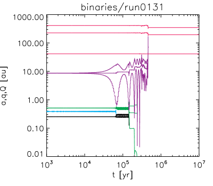
Figure 4: Ejection of the outer planet by the combined effects of the inner system and the stellar binary. After the outer planet’s pericentre reaches the inner system, scattering off the inner planets begins to raise its semi-major axis, ultimately leading to strong interaction with the binary and subsequent ejection.

Overall in our Binaries simulations, we lost 80 out of 400 outer planets: 43 were ejected, 35 hit the star, and 2 hit a more massive inner planet. In addition, 2 hit a less massive inner planet and survived. Considering only planets more massive than Saturn (194/400), we lost 32: 18 ejected and 14 hit the star, while 2 were hit by less massive inner planets and survived. Ejection of the outer planet can follow a similar route to that described in Mustill et al. (2015): despite having a larger mass than the inner planets, a highly-eccentric planet with a large semi-major axis can have less orbital binding energy than the lower-mass inners, and comparatively small changes to the semi-major axes of the latter can cause a large change to semi-major axis of the former. An example is shown in Figure 4, where the ejection of the outer planet is finally secured by the binary star after the inner planets have raised its semi-major axis.

4.2 Effects on inner system

4.2.1 Intrinsic multiplicities

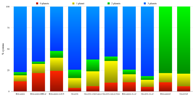
Figure 5: Multiplicities of inner systems arising from our simulation sets. See text and caption to Table 1 for a description of the simulation sets.

Integration set	$N_{\mathrm{sys}}$	$N_{0\mathrm{p}}$	$N_{1\mathrm{p}}$	$N_{2\mathrm{p}}$	$N_{3\mathrm{p}}$
Binaries	400	46 ($11.7\pm 1.6\%$)	28 ($7.2\pm 1.3\%$)	14 ($3.7\pm 0.9\%$)	312 ($77.9\pm 2.1\%$)
Binaries-E$>0.5$	185	44 ($24.1\pm 3.1\%$)	28 ($15.5\pm 2.6\%$)	14 ($8.0\pm 2.0\%$)	99 ($53.5\pm 3.6\%$)
Binaries$>$Msat	194	42 ($21.9\pm 2.9\%$)	21 ($11.2\pm 2.2\%$)	5 ($3.1\pm 1.2\%$)	126 ($64.8\pm 3.4\%$)
Giants	400	15 ($4.0\pm 1.0\%$)	46 ($11.7\pm 1.6\%$)	38 ($9.7\pm 1.5\%$)	301 ($75.1\pm 2.2\%$)
Giants-unstable	259	15 ($6.1\pm 1.5\%$)	45 ($17.6\pm 2.4\%$)	35 ($13.8\pm 2.1\%$)	164 ($63.2\pm 3.0\%$)
Giants-selected	39	4 ($12.1\pm 5.0\%$)	10 ($26.7\pm 6.8\%$)	2 ($7.3\pm 4.0\%$)	23 ($58.5\pm 7.6\%$)
Binaries-flat	300	31 ($10.6\pm 1.8\%$)	28 ($9.6\pm 1.7\%$)	15 ($5.3\pm 1.3\%$)	226 ($75.2\pm 2.5\%$)
Giants-flat	300	15 ($5.3\pm 1.3\%$)	24 ($8.3\pm 1.6\%$)	12 ($4.3\pm 1.2\%$)	249 ($82.8\pm 2.2\%$)
Binaries2	300	31 ($10.6\pm 1.8\%$)	32 ($10.9\pm 1.8\%$)	237 ($78.8\pm 2.3\%$)	-
Giants2	300	17 ($6.0\pm 1.4\%$)	44 ($14.9\pm 2.0\%$)	239 ($79.5\pm 2.3\%$)	-
Binaries-0pl	200	0 ($<1.5\%$)	4 ($2.5\pm 1.1\%)$	1 ($1.0\pm 0.7\%$)	195 ($97.0\pm 1.2\%$)
Giants-1pl	200	0 ($<1.5\%$)	0 ($<1.5\%$)	0 ($<1.5\%$)	200 ($>98.5\%$)

Table 1: Number of simulations per set ($N_{\mathrm{sys}}$), and numbers with a given number of inner planets after 10 Myr integrations ($N_{n\mathrm{p}}$). Binaries have 3 inner planets, one outer from 1 to 10 au, and a binary companion; Binaries$>$tkoz is the subset of these where the integration time exceeded the Kozai time-scale; Binaries$>$Msat the subset where the outer planet’s mass is greater than Saturn’s. Giants have three inner planets and four outer planets; Giants-unstable is the subset of these that lost at least one giant planet; Giants-selected is a subset of Giants chosen to have an eccentricity distribution consistent with the observed population. flat systems have initially zero mutual inclination between the inner planets (binary companions remain isotropically distributed). Binaries2 and Giants2 have initially only two inner planets. Binaries-0pl has a Kepler triple-planet system, a binary companion, but no extra planet, while Giants-1pl has a Kepler triple-planet system and a single outer giant planet. Percentages in brackets give the mean and standard deviation for the occurrance rate of each outcome from inverting the binomial distribution. $3\sigma$ upper/lower limits are given where appropriate.

The majority of our inner planetary systems remain stable in the Binaries simulations: 312/400 retain all three inner planets, while 15 are reduced to double-planet systems, 28 to singles, and 45 are cleared of all planets with $P<240$ d. These statistics are tabulated in Table 1 and displayed graphically in Figure 5; Figure 1 shows the outcomes as a function of the masses and semimajor axes of bodies in the system. Tighter binaries are more destabilising, as are more massive outer planets. The more distant outer planets are also more destabilising for the inner system; this is attributable to their Kozai cycles not being quenched by the inner planets, as explained above. Of the inner planets lost, $52\%$ collide with the star, $5\%$ are ejected, while $43\%$ are lost to inelastic planet–planet collisions. If we restrict attention to only those systems where the outer planet attains a maximum eccentricity of at least 0.5 (Binaries-e$>$0.5 in Figure 5 and Table 1) then the fraction of destabilised inner systems rises to almost 50%. If we consider systems where the outer planet is more massive than $3\times 10^{-4}\mathrm{\,M}_{\odot}$, we find around 1 in 3 inner systems destabilised (Binaries$>$Msat in Table 1, with 126 of 194 triple-planet systems remaining triples, 5 being reduced to doubles, 21 to singles and 42 with no surviving inner planet).

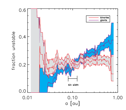
Figure 6: Rates of destabilisation as a function of the inner planets’ semi-major axes. Stability is counted as a property of the whole inner system, so for example a system with planets at $0.1$, $0.3$ and $0.5$ au, which loses the outermost planet, contributes to the destabilisation fraction at all three radii. We show the fraction for running bins of the indicated width, together with $1\sigma$ confidence intervals. The Binaries simulations are equally destructive to all inner systems, whereas the Giants simulations are less destructive the smaller the inner system’s semimajor axis.

The destabilisation fraction of $20-25\%$ is approximately constant across the range of semimajor axes of the inner planets: Figure 6 shows the fraction of inner planets with given initial semimajor axes that reside in systems that lose at least one inner planet, which is relatively flat, in contrast to the Giants simulations, which we discuss in the next section. This flatness can be understood in terms of the minimum pericentre of the outer planet (Figure 3): if Kozai cycles are excited in the outer planet, it is easy for the pericentre to attain a very low value (roughly as many outer planets attain $q_{\mathrm{min}}<0.1$ au as $q_{\mathrm{min}}\in[0.1,1]$ au). Destabilisation of the inner system can sometimes occur when the outer planet’s pericentre does not come inside the initial semimajor axis of the inner planet, this occurring in 19% of unstable inner systems (Figure 3, bottom right panel).

Our simulations permit us to verify the main result of Mustill et al. (2015), where we showed that a highly-eccentric proto-hot Jupiter would quickly destroy any other planets in the inner system, before tidal circularisation could change its orbit. In 11 simulations in Binaries, an outer planet attained a pericentre less than $0.05$ au at some point during the integration, while not being destroyed by ejection or collision. In all of these systems, the three inner planets were lost, mostly by collision with the star, and in 9 cases this occurred within 1 Myr, long before tidal circularisation would cause the outer planet to become a hot Jupiter.

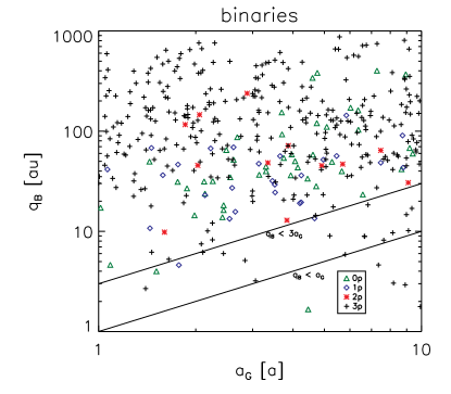
Figure 7: For outer planets with $M>10^{-4}\mathrm{\,M}_{\odot}$, we show the initial semi-major axis of outer planet $a_{\mathrm{G}}$, pericentre of binary $q_{\mathrm{B}}$, and resulting number of inner planets. We also show the line where the binary’s pericentre reaches one or three times the outer planet’s orbit; this latter is an approximate stability limit for hyperbolic 3-body encounters (e.g., Pfalzner et al., 2005).

We note that a small number of our systems are set up with the binary on an initial orbit taking it very close to the planetary region, due to the high eccentricities that can be randomly assigned. The binary pericentres, and the initial semi-major axes of the giant outer planets, are shown in Fig 7. Some binary companions overlap with or come within a factor of a few of the orbit of the outer planet, but this does not lead to a higher rate of destabilisation of the inner systems; giant planets in these systems are however removed considerably more quickly than in those with higher binary pericentres: the median time to ejection of the outer planet in systems with $q_{\mathrm{B}}<3a_{\mathrm{G}}$ was only $24$ kyr compared to $1.06$ Myr in systems with $q_{\mathrm{B}}>3a_{\mathrm{G}}$ While seemingly implausible in the context of planet formation in these systems, systems such as this might arise if binary orbits are changed or stellar companions exchanged by encounters with other stars in a cluster (e.g., Malmberg et al., 2007b).

4.2.2 Effects on mutual inclinations

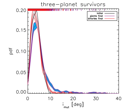
Figure 8: Top: Final mutual inclinations of adjacent inner planet pairs in the Binaries and Giants simulations, for systems that end with three inner planets. The initial distribution is also shown. Bottom: Final mutual inclinations in the systems that end up with two planets. Here we combine Giants with Giants-flat, and Binaries with Binaries-flat, for better statistics. We also show the range of mutual inclinations inferred for Kepler-108 (Mills & Fabrycky, 2016). We also show with dashed lines the initial 2-planet systems (Binaries2 and Giants2).

Direct loss of inner planets is the most violent but not the only effect the outer system can have on the inner. The mutual inclinations of the inner planets can also be affected. In Figure 8 we show the instantaneous mutual inclinations of surviving 3-planet systems from Binaries at 10 Myr. While the bulk of the distribution is close to the initial distribution (between $0^{\circ}$ and $10^{\circ}$), a small number of systems are excited to a higher mutual inclination of up to $20^{\circ}$. The outer planet is incapable of exciting high mutual inclinations amongst the inner planets through secular means, as the inner planets typically are coupled together too strongly. We use Equation 29 of Lai & Pu (2016) to parametrise the strength of the inclination forcing from the outer planet compared to the coupling between the inner planets (their $\bar{\epsilon}$ we call $\epsilon$). $\epsilon\ll 1$ implies strong coupling between inner planets with little excitation of mutual inclinations, while $\epsilon\gg 1$ implies that the outer planet dominates, allowing mutual inclinations amongst the inners to be excited to up to twice the initial value of that between the inners and the outer planet. Secular resonance can exist in the region $\epsilon\sim 1$ that can excite still higher values of mutual inclination (Lai & Pu, 2016). All of our surviving triple-planet systems have $\epsilon<1$, with many around $10^{-3}$, and hence the outer planet cannot efficiently drive up mutual inclinations in the inner system. Similar results hold for the other integration sets.

More interesting is the case of two-planet survivors, which shows a larger tail of systems of high mutual inclination of up to $60^{\circ}$ (Figure 8, bottom panel). This provides a means of generating misaligned systems such as Kepler-108 (Mills & Fabrycky, 2016), as we discuss below. The systems initially with two inner planets (Binaries2 and Giants2) that retain both are less excited, as is shown by the dashed lines.

In summary, Kozai perturbations to outer planets disrupt inner systems in around $20-25\%$ of cases. Mutual inclinations of surviving triple-planet systems remain unexcited, but destabilised systems reduced to two planets can become mutually inclined up to several tens of degrees.

5 Population synthesis II: Scattering

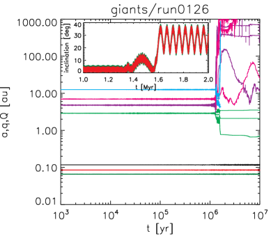
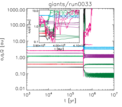
Figure 9: Example evolution of Giants systems, showing the semi-major axis, pericentre and apocentre of all bodies. The inner Kepler triple-planet system is in dark green, red and black, while the four outer planets are in light green, purple, magenta and cyan. Left: Scattering in the outer system leaves the inner planets dynamically cold but induces a significant obliquity on the whole inner system; inclinations of the inner planets are shown in the inset. Right: A contribution to the Kepler dichotomy: a single inner planet survives after scattering in the outer system induces scattering in the inner system. The inset shows a zoom-in around the strong scattering at $\sim 0.4$ Myr.

Examples of the effects of scattering in the outer system in the Giants simulations are shown in Figure 9. In the left panel, strong scattering leaves the inner system dynamically unexcited but induces a large obliquity on the set of three planets. In the right panel, we see a contribution to the Kepler Dichotomy: the inner system is destabilised once scattering begins in the outer system and eventually only a single planet is left in the inner system. We now describe this integration set in more detail.

5.1 Effects on outer system

Of our 400 systems, 141 were stable and retained all their giant planets. 120 lost one giant, 130 two, and 9 lost three. One of the systems that retained its four giants was undergoing scattering at the end of the integration, with one planet having been ejected onto a wide ($a=120$ au, $e=0.9$) orbit.

In addition to Kozai cycles, planet–planet scattering followed by tidal circularisation has also been proposed as a migration channel for hot Jupiters (Rasio & Ford, 1996; Weidenschilling & Marzari, 1996; Nagasawa et al., 2008; Beaugé & Nesvorný, 2012). Combining N-body integrations with tidal forces, Nagasawa et al. (2008) found that 30% of unstable 3-planet equal-mass systems form hot Jupiters, while with a small spread in masses (a factor 4 at most) Beaugé & Nesvorný (2012) found that 10% of unstable three-planet and 23% of four-planet systems form hot Jupiters. Our potential hot Jupiter formation rate—planets hitting the star, as well as planets attaining small pericentres—is much smaller, only a few per cent. (Figure 3, bottom right). We attribute this to the broader range of masses we use for the outer planets: in more hierarchical systems, the lower-mass planets can be ejected without the remaining large planets acquiring significant eccentricities, and equal-mass systems are far more disruptive to other bodies in the system (Carrera et al., 2016).

We also found that the eccentricities of our surviving outer planets were lower than the observed population of giant exoplanets. We therefore construct a Giants-selected sample from our simulations in the following manner. We construct an empirical eccentricity distribution from www.exoplanets.org (Han et al., 2014) for RV-discovered planets with mass greater than Saturn’s and period greater than 50 days, and also construct the distribution for our surviving planets in the same mass range (Figure 10, upper panel). We divide this up into 10 eccentricity bins of width $0.1$, assign each bin a weight of $N_{\mathrm{empirical}}/N_{\mathrm{modelled}}$, and normalise the weights so that the maximum is unity. For each model planet we then add it to our sample with a probability equal to its bin weighting. Thus, systems in a bin which is over-represented in the simulations will be assigned a low probability of being selected. In doing this, we reduce the size of our sample by a factor of roughly 10, but we avoid resampling the same system multiple times. This results in the Giants-selected distribution shown in the upper panel of Figure 10, with 39 selected systems. The final states of these systems are displayed in the lower panel of Figure 10.

5.2 Effects on inner system

5.2.1 Intrinsic multiplicities

Unsurprisingly, in the systems that retained all their giants, the inner system was nearly always unperturbed: only 4 of these 141 systems lost one of their KOIs, suggesting that long-range dynamical excitation (through secular resonances for example) is inefficient at destabilising inner systems, unless at least a moderate degree of excitation is reached in the outer system (the mean final eccentricity among the outer planets in these systems was $0.017$, and the median $0.006$), although our 10 Myr integrations may miss instabilities that could occur on timescales of several Gyr. More significantly, most of the unstable giant systems also retained their three KOIs in the inner system: only $95/259=37\%$ of the unstable systems lost one or more of their KOIs. Thus, even in dynamically active outer systems, destabilisation of the inner system occurs in roughly only 1 in 3 cases. Our Giants-selected runs are less hierarchical than their Giants superset, with a median mass ratio of $2.1$ vs $2.7$. Unsurprisingly, they are also more destructive of the inner systems than Giants, keeping only $58.5\pm 7.6\%$ of inner triple-planet systems intact, compared to $75.1\pm 2.2\%$ for Giants and $63.2\pm 3.0\%$ for Giants-unstable. Of the inner planets lost, $51\%$ hit another planet, $38\%$ collided with the star, and $12\%$ were ejected. Though the number of events is small (21 ejections here, compared to 11 in Binaries), the larger fraction of ejections in the Giants simulations may be a signature of the “uplift” mechanism we discuss in the context of eccentric warm Jupiters in Section 6.3.

In contrast to Binaries, the fraction of destabilised inner systems rises with the semimajor axis of the inner planet (Figure 6). The outer planets in Giants rarely achieve such small pericentre as in our Kozai simulations (Figure 3, bottom-right panel), and only 11 outer planets managed to collide with the star here, compared to 35 in Binaries. In most cases of destabilisation of the inner system one or more of the outer planets’ pericentres comes within the semimajor axis of the outermost inner planet (Figure 3, bottom-right panel, purple lines). However, in a minority of cases destabilisation occurs at a distance, without any outer planet’s orbit penetrating the initial semimajor axes of the inner planets. This is more common in Giants than in Binaries, occurring in 34% of cases of instability compared to 19%. This suggests that secular effects are more effective at exciting the inner system: as discussed in Matsumura et al. (2013) and Carrera et al. (2016), as outer giant planets undergo scattering, secular resonances can jump around the inner system, exciting eccentricities of inner planets without the outer giants actually approaching the inner planets closely.

The stable inner systems experience a small degree of dynamical excitation. In Figure 11 we show the eccentricity distribution of surviving triple KOIs, broken down by the number of surviving giants. While there is a trend towards higher eccentricities for more violent instabilities (as measured by the number of surviving giants), eccentricities remain low: in the unstable giant planet systems, 90% of the KOIs in systems that retain all three of the inner planets have $e<0.09$ at the end of the integration. This comports with the majority of observed multi-planet Kepler systems which appear to have similarly low eccentricity (Van Eylen & Albrecht, 2015).

5.2.2 Mutual inclinations

Effects on mutual inclinations are broadly similar to the Binaries runs, with little excitation among the triple-planet survivors (Fig 8, top). The 2-planet survivors are more excited than are the 2-planet survivors in Binaries (Fig 8, bottom), although the sample size here is smaller. Interestingly, we see no correlation of the mutual inclination of the two-planet systems with the minimum pericentre attained by any of the giant planets, suggesting that in some systems at least the destabilisation and eccentricity excitation is a result of secular effects and not direct scattering by the outer planets. Secular effects could be amplified if secular resonances jump around the inner system during scattering among the outer planets (Matsumura et al., 2013; Carrera et al., 2016).

The diversity of final inclinations is shown in Figure 12. Here we show, for surviving double- and triple-planet systems, the mutual inclinations between adjacent planet pairs against the inclination of each planet with respect to the initial reference plane (each system is thus represented by two or four points). Systems start in the dark shaded lower left quadrant. A small number move rightwards, increasing the system’s inclination while keeping mutual inclinations low, to form systems similar to Kepler-56. Other systems, often those destabilised and reduced to double systems, move upwards and rightwards, gaining a mutual inclination instead of remaining coplanar.

In contrast to the Binaries case, flattening the planetary system does have an effect on the inner system. This is because by flattening the outer system as well, a larger fraction of systems experience collisions between the outer planets (64 cases in 300 systems, compared to 39 cases in 400 systems), while only 3 outer planets collide with inner planets, compared to 10 in the non-coplanar Giants runs, despite the flatness of the systems.

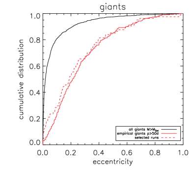
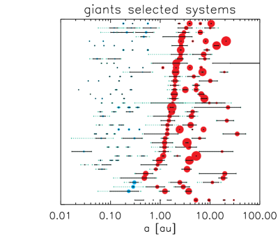
Figure 10: Top: Eccentricity distributions of surviving planets more massive than Saturn in our Giants runs, the empirical distribution for planets in the same mass range and $P>50$ days, and a subset of the former drawn to be consistent with the latter. This subset (Giants-selected) is constructed by dividing the observed and simulated giant planets into eccentricity bins, assigning each bin a weight according to how over-represented it is in the simulations, and randomly drawing simulated systems to give the same eccentricity distribution as the observed one. See §5.1 for details. Bottom: Masses, semimajor axes and eccentricities of the Giants-selected systems at 10 Myr. Symbol size is proportional to the cube root of planet mass, and the Solar System is shown at the bottom for reference. Solid lines show the final eccentricity, dashed lines the greatest eccentricity attained. Blue planets are initially inner KOIs, while red planets are initially outer giants.

Figure 11: Eccentricities of surviving triple-planet KOI systems separated according to the number of surviving giants in the outer system. We also include the final eccentricities of KOIs in the Control sample without any additional bodies (§2). KOIs in systems of stable outer giants have their eccentricities excited by a factor of $\sim 10$, but they remain low in absolute terms (median $\sim 10^{-3}$). Unstable outer systems excite eccentricities more the more planets they lose.

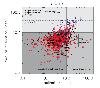
Figure 12: Final inclinations and mutual inclinations of surviving inner double- and triple-planet systems from Giants. On the $x$-axis, the inclination of each planet with respect to the original reference plane is shown. On the $y$-axis, the mutual inclination of each pair of adjacent planets is shown. Hence, each planet pair contributes two points, at identical $y$-values. Systems begin in the lower left quadrant with $i_{\mathrm{mut}}<10^{\circ}$. They may subsequently be excited to high mutual inclination (more common when the multiplicity itself is reduced to a double system), or gently tilted to a high inclination with respect to the system’s original invariant plane, while maintaining a low mutual inclination. We also mark the system Kepler-56 (Huber et al., 2013).

6 Formation of eccentric warm Jupiters

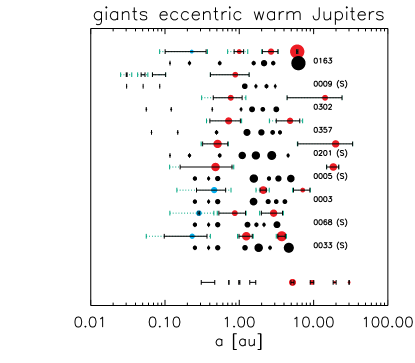
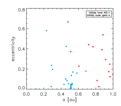
Figure 13: Top: Formation of eccentric warm Jupiters in our Giants integrations. We show systems with at least one planet with mass greater that that of Saturn, semi-major axis less than 1 au, and eccentricity greater than 0.3 at any point between the time the final planet was removed and the end of the integration. The dotted lines show the maximum eccentricity of each planet attained during this time, while solid lines show the instantaneous eccentricity at the end of the integration. Red planets are originally outer planets while blue are originally inner Kepler planets. Circle radius is proportional to the cube root of mass. Below each final system, we show in black the initial configuration. Run IDs are noted; see text for discussion of some individual systems. Runs marked “(S)” are in the Giants-selected sample. The Solar System is shown at the bottom for comparison. Bottom: All warm Jupiters (including those with $e<0.3$) at the end of our Giants simulations. Eccentricity is plotted against semimajor axis for each planet with a mass greater than Saturn’s and a semimajor axis $<1$ au. Planets that are originally one of the triple KOIs are shown in blue, while those originally an outer giant are in red.

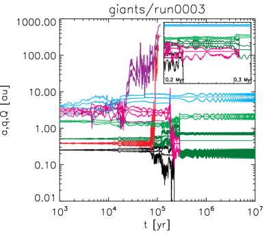
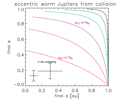
Figure 14: Left: Formation of an eccentric warm Jupiter by an inelastic collision between two $\sim$Saturn-mass planets, the interior on a low-eccentricity orbit and the exterior on a high-eccentricity orbit (inset, at $0.285$ Myr). Right: Toy model of the formation of eccentric warm Jupiters through inelastic planet–planet collisions. A Jupiter-mass planet is placed at 1 au with another planet interior, with mass ranging from Earth-mass to Jupiter mass and semimajor axis from $0.01$ to 1 au. The giant planet is given sufficient eccentricity for its pericentre to reach the inner planet’s orbit. The semimajor axis and eccentricity of the merger product are shown, assuming that this merger occurs at pericentre and conserves mass and angular momentum. Each line shows a different mass of the inner planet; lines terminate at an inner planet’s $a=0.01$ au. Each line thus shows the locus $(a_{\mathrm{f}}(a_{1};m_{1}),e_{\mathrm{f}}(a_{1};m_{1}))$ for a given $m_{1}$: see Equations 10 and 11. Crosses show eccentricities attained from in-situ scattering (Petrovich et al., 2014).

An interesting challenge to models of planet migration and dynamics has been raised by the discovery of a population of eccentric warm Jupiters at separations of a few tenths of an au. We may divide warm Jupiters into three eccentricity ranges:

1. Low eccentricity: These are consistent with disc migration and/or in situ formation. In reality the two are connected, since planets accrete as they migrate: see for example the growth tracks in Figure 2 of Bitsch et al. (2015). These planets can acquire low eccentricities through in situ scattering, but Petrovich et al. (2014) show that eccentricities of above $0.3$ are very hard to attain because planets on close-in orbits preferentially collide before they acquire higher eccentricities. We therefore take $e=0.3$ as the upper eccentricity bound for this sub-population.

2. Super eccentricity: These are warm Jupiters with small pericentres moving down tidal circularisation tracks, and would, in time, become hot Jupiters (Socrates et al., 2012; Dawson et al., 2015). The tidal migration rate is a very strong function of the planet’s pericentre distance, and we may take $q\approx 0.04$ au to define an envelope in $a-e$ space below which tidal migration cannot populate (without additional forcing; see the next point).

3. Moderate eccentricity: Lying in the eccentricity range between these two extremes, the moderately-eccentric warm Jupiters have eccentricities too high to be produced by in situ scattering but too low to be following a tidal circularistaion track. Proposed formation mechanisms include the “slow” regime of Kozai cycles plus tidal friction, during which eccentricity oscillations still occur while tidal dissipation happens only at eccentricity maxima (e.g., Dawson & Chiang, 2014; Dong et al., 2014; Petrovich & Tremaine, 2016), and inelastic collisions between eccentric giant planets from the outer system and sufficiently massive inner planets (Mustill et al., 2015).

Here we focus on the moderately-eccentric population with $e>0.3$ and $q>0.04$ au, elaborating on the inelastic collision mechanism of Mustill et al. (2015) and describing two further formation channels for these objects.

Defining such planets as those more massive than Saturn, with semimajor axis less than 1 au, and which attain an eccentricity of at least $0.3$ at some point after the loss of the final planet, we find eccentric warm Jupiters to be produced in 9 of our Giants simulations, and 3 of our Binaries simulations.

The systems from the Giants simulations are displayed in Figure 13. This formation rate ($9/400=2.5\pm 0.8\%$) is low, but is higher for our Giants-selected sample at $5/39=14.6\pm 5.5\%$; selected systems are indicated in Figure 13. Four of our eccentric warm Jupiter systems (with the smallest semimajor axis of the warm Jupiter: the lowest four systems in Figure 13) share a common KOI inner triple-planet system: KOI620, alias Kepler-51. With our adopted mass–radius relation, this system has planet masses of $2.1\times 10^{-4}$, $3.8\times 10^{-4}$, and $8.3\times 10^{-5}\mathrm{\,M}_{\odot}$. Three of the eccentric warm Jupiters in Giants were originally members of inner systems, while the remaining 6 were initially outer planets. We also show in the bottom panel of Figure 13 the eccentricities and semimajor axes of all planets more massive than Saturn with $a<1$ au at the end of the simulation. Most of these warm Jupiters that originated as one of the triple KOI inner planets retain a low eccentricity, while those originating as outer planets have a broader range of eccentricities. This underlines the $e>0.3$ criterion we used to distinguish the low-eccentricity from the moderate-eccentricity warm Jupiters.

We now discuss the formation of these eccentric warm Jupiters. We identify three pathways: inelastic collision between an inner planet and an eccentric outer planet as in Mustill et al. (2015) (Section 6.1); secular forcing, possibly involving freezing into a high-eccentricity state as scattering resolves (Section 6.2); and in-situ scattering, which may be aided by “uplift” as one planet is removed from the inner system by the outer planets (Section 6.3).

6.1 Eccentric warm Jupiters from inelastic planet–planet collision

In Mustill et al. (2015) we found that a highly-eccentric Jupiter-mass planet experiencing an inelastic collision with an inner Neptune-mass planet can form an eccentric warm Jupiter, which is the merger product of the two planets. While that study was an idealized case of the giant’s eccentricity being imposed arbitrarily, rather than arising consistently through dynamical evolution, this mechanism remains at work when we treat the dynamics consistently in the present study, and two of our eccentric warm Jupiters form from such inelastic collisions. We show one example in the left-hand panel of Figure 14: after a period of scattering, in which two roughly Saturn-mass planets switch places, the eccentricity of the outer one of the pair is excited to almost $0.8$, and it then collides with the inner, causing its semi-major axis to shrink from $\sim 0.9$ au to $0.46$ au, and leaving its eccentricity stably oscillating around $0.6$.

We construct a toy model of this process as follows. Assume that a giant planet at a semi-major axis $a_{2}$ with mass $m_{2}$ is given sufficient eccentricity to collide with a coplanar planet of mass $m_{1}$ on a circular orbit at $a_{1}<a_{2}$, and that the planets then collide inelastically before their orbits change further, conserving mass and angular momentum. The angular momenta of the two planets before the collision are

$$L_{1}=m_{1}\sqrt{\mathcal{G}M_{\star}a_{1}},\qquad L_{2}=m_{2}\sqrt{\mathcal{G}M_{\star}a_{1}(1+e_{2})}.$$ (9)

The final eccentricity of the merger product is then given by

$$e_{\mathrm{f}}=\left(\frac{m_{1}/m_{2}+\sqrt{1+e_{2}}}{m_{1}/m_{2}+1}\right)^{2}-1,$$ (10)

guaranteed to lie between 0 and the initial eccentricity $e_{2}$, while the final semi-major axis is

$$a_{\mathrm{f}}=\frac{a_{1}}{1-e_{\mathrm{f}}},$$ (11)

lying between the initial semi-major axes $a_{1}$ and $a_{2}$. The final $a$ and $e$ of the merger products are shown in the right-hand panel of Fig 14, for $a_{2}=1$ au, $m_{2}=10^{-3}\mathrm{\,M}_{\odot}$, and a range of $a_{1}$ and $m_{1}$. An inelastic collision of the eccentric Jupiter with a super-Earth at 0.01 au is sufficient to shrink the giant’s orbit by a factor of 2, although collision with an object more massive than Neptune would be required to simultaneously reduce the eccentricity below $0.9$.

This mechanism was also responsible for producing one of the eccentric warm Jupiters in our Binaries simulations: that shown in the left panel of Figure 2. Here however, the warm Jupiter possesses a very small pericentre after the collision, meaning that the warm Jupiter phase would only be transient and the planet would in time circularise to become a hot Jupiter.

6.2 Eccentric warm Jupiters from secular chaos and secular freeze-out

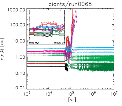
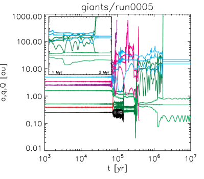
Figure 15: Formation of eccentric warm Jupiters by secular processes. Left: As a result of planet–planet scattering, significant angular momentum defict is generated, allowing the inner planet’s eccentricity to be forced up by secular processes (initially at around $0.09$ Myr; see inset). Secular cycles continue for the remainder of the integration, with irregular modulation. Right: After the initial scattering ends at around $0.4$ Myr, the warm Jupiter’s eccentricity is first forced by the second remaining planet (inset). This forcing ends however when this planet is itself ejected by the third survivor, causing the warm Jupiter to be “frozen” into a high-eccentricity state, with the mutual inclination between the two surviving planets at $\sim 80^{\circ}$.

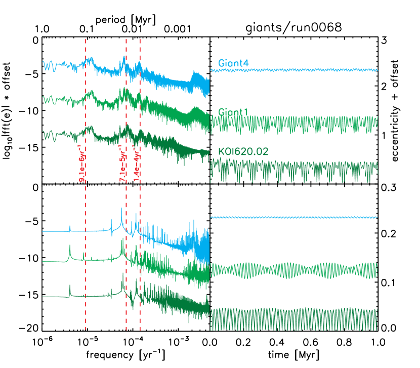
Figure 16: Further evolution the system shown in the left panel of Fig 15. Top: The system is integrated for a further 10 Myr; the first 1 Myr of eccentricity evolution is shown on the right and the FFT of the full 10 Myr on the left. The strongest peaks are near the frequencies predicted by leading-order Laplace–Lagrange secular theory (red), but the breadth of the peaks is indicative of chaotic behaviour. Bottom: Here the system is initially identical in all orbital elements but the eccentricity is reduced by a factor of 10. Peaks in the periodogram are now narrow and distinct, indicative of regular quasiperiodic motion.

Some warm Jupiters in our simulations are produced by a combination of secular processes and scattering. In Giants/run0068, planet–planet scattering generates significant angular momentum deficit which results in the three surviving planets having significant eccentricities, the inner two in particular experiencing large irregular oscillations (Fig 15). The chaotic nature of the subsequent secular evolution is revealed in Fig 16, where we extend the integration run for a further 10 Myr. We compare the evolution of the system continued from the end of our simulation with one identical in all orbital elements except that eccentricities are reduced by a factor of 10. In the low-eccentricity case, power in the periodogram of the eccentricity evolution is concentrated at well-defined peaks close to the frequencies predicted by Laplace–Lagrange secular theory, characteristic of regular quasiperiodic motion. In contrast, in the high-eccentricity system that arises from our initial integration, these peaks are significantly broadened, characteristic of chaotic motion.

A second variant of secular warm Jupiter formation is shown in the right-hand panel of Figure 15. Here an unstable three-planet system arises from the initial scattering, with the warm Jupiter the innermost of the three. Its eccentricity is initially forced by the second of the planets during the latter’s phases of high eccentricity, a process which ends when the third survivor ejects this planet at around $1.8$ Myr. The warm Jupiter is then frozen into a high-eccentricity state, experiencing weak Kozai forcing largely suppressed by general relativistic precession (mutual inclination of approximately $80^{\circ}$). This mechanism, whereby the warm Jupiter acquires its eccentricity by secular forcing from an outer system which is itself unstable and whose evolution ends following the ejection of all but one body, we dub “freeze-out”.

6.3 Eccentric warm Jupiters from in-situ scattering and uplift

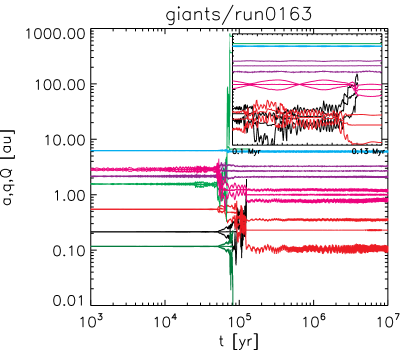
Figure 17: Formation of an eccentric warm Jupiter (pink; second surviving planet) and an eccentric sub-Saturn (red; innermost surviving planet). The initially second and third (black and red) planets undergo a phase of scattering between $0.1$ and $0.12$ Myr, which ends when the black planet interacts with the pink planet just beyond 1 au, raising its pericentre to detach it from the innermost planet, a process we call “uplift” (inset). The innermost sub-saturn is left with an eccentricity fluctuating between $0.5$ and $0.6$, while the warm Jupiter’s eccentricity varies between $0.11$ and just over $0.3$.

Planets undergoing scattering at a few tenths of an au are inefficient at exciting high eccentricities or causing ejections, as their gravitational focusing is reduced owing to the high orbital speeds (Petrovich et al., 2014). Instability in such systems usually leads to collisions and relatively low eccentricities of the surviving planets. Indeed, the only eccentric warm Jupiters we formed directly by in-situ scattering, which had $a$ just under $1$ au, arose from giant outer planets scattering each other, not from scattering in the more massive of the inner systems.

However, we find that the addition of outer giant planets can enhance the rate of ejections of planets from the inner system. Of our 22 Giants systems modelled on KOI620 that were unstable, 13 of them ejected an inner planet. We ran 100 systems based on KOI620 with no outer planets and small separations between the inner planets, and another 100 similar with the mutual inclinations reduced to $0.1^{\circ}$ as in Petrovich et al. (2014). Of these, only 12 out of 100 of the moderately-inclined and 9 out of 100 of the coplanar systems ejected an inner planet, despite all being unstable: the majority of planets lost suffered collisions with other bodies.

The presence of outer giants enhances the ejection rate by a process we call “uplift”: when an inner planet attains a moderate eccentricity, it can begin scattering off the outer planets, which can raise its pericentre out of the inner system, and ultimately lead to its ejection, while quickly decoupling it from the other inner planets before a physical collision occurs. An example is shown in Figure 17, where the second and third planets scatter each other until one is lifted out of the inner system by one of the outer planets, with which it collides shortly afterwards. This leaves the innermost surviving planet with a significant eccentricity of $0.5-0.6$; if scattering had continued between only the inner two planets; the probable outcome would have been a collision resulting in a lower eccentricity for the merger product. Although in this case the innermost planet is too low in mass ($1.4\times 10^{-4}\mathrm{\,M}_{\odot}$) to qualify as a warm Jupiter (the warm Jupiter here is actually the second planet, which just meets our criterion at $a=0.997$ au), this process should work more efficiently if the inner planet were higher in mass, as scattering to the outer system would then be easier, making this a viable route to produce eccentric warm Jupiters.

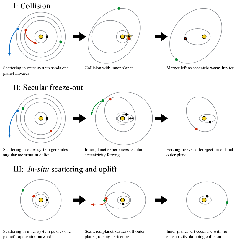
Figure 18: Cartoon summarising routes to the formation of eccentric warm Jupiters. Top: An outer giant is scattered into the inner system, where it collides with a close-in planet to lower its eccentricity (see Fig 14, Section 6.1 and Mustill et al. 2015). Middle: Scattering in the outer system generates angular momentum deficit (AMD), which periodically excites the inner planet’s eccentricity (see Fig 15 and Section 6.2). If scattering continues in the outer system, the inner planet’s eccentricity can be frozen into a high value after planetary ejections cease. Bottom: Scattering in the inner system leads to one planet’s apocentre being raised enough to interact with outer giants, which then decouples this planet from the inner system and prevents a collision with the other inner planet, which would generally reduce eccentricity (see Figure 17 and Section 6.3).

7 Discussion

7.1 Relation to previous work

We have studied several aspects of the interactions between outer planetary systems beyond 1 au and inner systems such as those discovered by Kepler. Our present work builds on the study of Mustill et al. (2015), wherein we showed that highly-eccentric giant planets en route to becoming hot Jupiters would clear inner planets out of the inner system. While in our previous study we imposed the high eccentricity at the beginning of the integration, in our present study we allow the eccentricity to arise naturally as a result of the dynamics of the outer system. We verify that these highly-eccentric planets also clear out their inner systems when we model the dynamics consistently: in our Binaries integrations, all 11 systems where the outer planet both attained a pericentre $<0.05$ au and survived to the end of the integration lost all other planets in the system.

A number of other authors have considered aspects of the effects of the dynamics of outer systems on inner ones. The study of the effects of planet–planet scattering on inner terrestrial planets in the habitable zone has a venerable tradition (e.g., Veras & Armitage, 2005, 2006; Raymond et al., 2011, 2012; Matsumura et al., 2013; Carrera et al., 2016; Kaib & Chambers, 2016). Our inner systems, being modelled on Kepler systems, are often closer to the star than the habitable zone, but an extrapolation of our Giants results suggests that $\sim 40\%$ of habitable-zone planets in unstable systems of giant planets would belong to inner systems that were themselves destabilised (Figure 6). This is somewhat less than the hierarchical case (4Gb+4e) studied by Carrera et al. (2016) where $70\%$ of habitable-zone planets were destabilised; most of this discrepancy is accounted for by the 141 of our outer systems that had not lost a planet during the course of the integration. A recent work by Huang et al. (2016a) studies the effects of scattering among giant outer planets on super-Earth systems, similar to our Giants-selected runs, finding a $70-80\%$ destabilisation rate, almost twice the value of ours. This may be attributable to their outer systems being closer to the inner systems than are ours.

Several groups have studied the effects that outer planets might have on the inclinations of inner systems. Lai & Pu (2016) find that an inclined outer planet can excite the mutual inclinations of Kepler systems, while Hansen (2016) finds that this process is greatly enhanced with two dynamically-excited outer planets, which can land secular resonances in the midst of the Kepler zone. Gratia & Fabrycky (2017) point out, in the context of Kepler-56, that such inclined outer planets can lead to an increase of the obliquity of an inner system without exciting mutual inclinations. Our study complements these works by treating consistently the origin of the eccentricities and inclinations of the outer planet(s).

We now proceed to discuss in more detail the effects on the multiplicities of Kepler systems, both in their intrinsic numbers of planets (Section 7.2.1) and in their mutual inclinations (Section 7.2.2); the generation of significant obliquities and mutual inclinations as seen in Kepler-56 and Kepler-108 (Section 7.3); and the formation of eccentric warm Jupiters (Section 7.4); before proceeding to critique our choice of initial conditions (Section 7.5), discuss neglected physical processes (Section 7.6) and consider the effects of long-term dynamical evolution (Section 7.7).

7.2 Sculpting the Kepler multiplicity function

7.2.1 Intrinsic multiplicities

The multiplicities of systems observed by Kepler depends on both the intrinsic multiplicity of the system and the mutual inclinations between the planets: a system with many planets but high mutual inclinations is more likely to only be observed as a single. Johansen et al. (2012) showed that the apparent excess of single-transit systems cannot be explained by varying the mutual inclinations of intrinsically triple-planet systems. Nor can internal dynamics of the triple-planet systems reduce multiplicity, as the surviving triple-planet systems are much too stable to be the survivors of a population with a continuous range of stability times, in contrast to higher multiplicity systems Pu & Wu (2015).

Given the prevalence of binary stellar companions and wide-orbit planets, we have explored the dynamical effects of these on Kepler-detected inner systems. We find that a reduction of the mutliplicity of the inner system occurs in $20-25\%$ of systems in our population syntheses. If we restrict our attention to a subsample of scattering planets chosen to have an eccentricity distribution matching observed exoplanets, the disruption rate rises to $\sim 40\%$; a similar rate is found for the systems with outer planets forced by binary companions to $e>0.5$. This is insufficient to explain the large excess of single-planet candidates from Kepler, especially when we consider that not all such systems will possess the necessary outer architectures.

However, violent dynamics in the outer system does make some contribution to the multiplicity function of inner systems. Assuming that the occurrence rates of system components are independent, we make the following estimates: For Binaries, around 25% of stars have a wide binary companion (Duchêne & Kraus, 2013), and microlensing suggests that $\sim 50\%$ of stars has a wide-orbit Neptune-mass planet or above. If 25% of such systems destabilise their inner systems, that gives a fraction of $\sim 3\%$ of inner systems destabilised by Kozai cycles induced on outer planets. For Giants, taking a giant planet occurrence rate of 20% as found by Uehara et al. (2016), noting that $\gtrsim 75\%$ of these may have undergone instability, and $40\%$ of these disrupt their inner systems (working with Giants-selected), we now end up with 6% of inner systems having been disrupted by an unstable outer system of giant planets.

These rates are clearly too low to reproduce the excess of single-planet Kepler systems. We note that unexplored architectures may raise this rate. In particular, we have not explored unstable systems of low-mass outer planets (almost all of our Giants runs possess at least one Saturn-mass planet). Scattering instabilities in low-mass systems take far longer to resolve than in high-mass systems (Mustill et al., 2016; Veras et al., 2016), and can result in large excursions in eccentricity and pericentre (Veras et al., 2016). While super-Earths or Neptunes penetrating the inner system directly would be less damaging than gas giant planets, and would probably simply result in the ejection of the intruder (Mustill et al., 2015), the longer timescales on which the scattering occurs would give more time for moving secular resonances to act on the inner system. If we assume that systems of unstable low-mass planets would be as disruptive as our Giants systems, we would estimate (raising the outer planet occurrence rate from $20\%$ to $50\%$) that 15% of inner systems are disrupted this way, for a total of 18% when adding the effects of the Binaries run: a significant contribution to the Kepler multiplicity function, but insufficient by itself to resolve the Kepler Dichotomy. The ratio of single to multiple planet Kepler systems is around 4:1 (Johansen et al., 2012), but as we find that only 18% of triple-planet systems are expected to be disrupted, this leaves over 75% of the single Kepler planets unaccounted for. From the outcomes in Table 1, we find about $10.6\%$ of Kepler triple-planet systems would be reduced to single-planet systems and around $6.0\%$ would lose all their planets. Unstable giants would contribute the most to this destabilisation, but binaries contribute more to the zero-planet systems than they do to the single-planet systems.

7.2.2 Mutual inclinations of inner planets

The observed multiplicity also depends on the mutual inclinations of the inner planets. Several recent papers have suggested that inclined outer planets can induce mutual inclinations in the inner systems that could help to generate an overabundance of single planet candidates and resolve the Dichotomy. Lai & Pu (2016) recently argued that inclined outer companions to Kepler multiple systems can excite large mutual inclinations through secular perturbations, leading to a large population of single-transit systems. We can look to see whether this effect occurs in our $N$-body runs.

Secular inclination forcing in the inner system depends on the strength of the coupling between inner planets compared to the forcing from the outer planet. Strong coupling between the inner planets means that high mutual inclinations cannot be excited. Lai & Pu (2016) parametrise this coupling with a parameter $\epsilon$ (their $\bar{\epsilon}$, Eq 29), where $\epsilon\ll 1$ means strong coupling and $\epsilon\gg 1$ means weak coupling. Secular resonances occur at $\epsilon\approx 1$ where very high mutual inclinations can be excited. However, in our integrations all of the systems had $\epsilon<1$.

To attain $\epsilon\geq 1$ the outer planets would have to be brought closer to the inner systems. While this is possible (note the gaps between the inner and outer systems in Fig 1), the inclination of the outer body or bodies with respect to the inner system must still be excited. It is possible that in this case the inclinations of the inner planets would be directly excited by scattering during the excitation of the outer system.

We do find a small number of mutually-misaligned two-planet survivors from the initial triple-planet systems (Figure 8): as in Spalding & Batygin (2016), who argued for secular inclination driving as a young star spins down, and Hansen (2016), who treated less violent outer system dynamics than we, significant inclinations are concomitant with dynamical instability. However, these systems are a small fraction of our full set of runs and cannot contribute significantly to the Kepler Dichotomy.

7.3 Tilting and strongly misaligning inner systems

However, in occasional cases these inclination effects are of interest. We draw comparisons to two observed systems of interest: Kepler-56 (Huber et al., 2013) and Kepler-108 (Mills & Fabrycky, 2016).

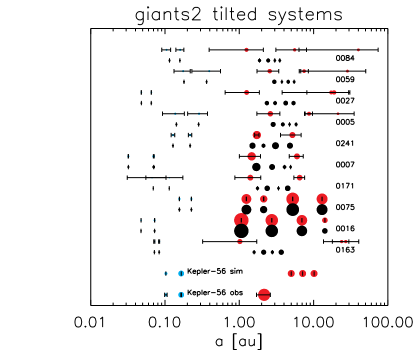
Figure 19: Systems of initially two inner planets resulting in orbits coplanar with each other but inclined away from the original reference plane, similar to Kepler-56, from the Giants2 simulations. The bottom rows show the observed Kepler-56 system from Otor et al. (2016), as well as the initial conditions for the simulations of Mills & Fabrycky (2016). In the two stable simulations with four surviving outer planets, the inner planets lie close to strong secular inclination resonances.

Kepler-56 is a system of two transiting planets (Huber et al., 2013) with a third planet at detected by RV at $2.1$ au, and likely no other giant planets within 20 au (Otor et al., 2016). The two inner planets have a misalignment with the host star of at least $45^{\circ}$ Huber et al. (2013), while having a low mutual inclination; the inclination of the outer planet is unknown. Li et al. (2014) showed that the high obliquity of the inner planets could be explained by an inclined outer giant planet; we have shown that this can indeed occur naturally, albeit somewhat rarely, as a result of scattering in the outer system. Successful examples (mutual inclination of the inner planets $<10^{\circ}$, and an absolute inclination of the innermost $>20^{\circ}$, at the end of the integration) from our Giants2 simulations are shown in Figure 19, together with the observed system. Gratia & Fabrycky (2017) also successfully achieved the mutual inclinations with scattering between three equal-mass giant planets, as marked on the Figure. The equal mass case results in the most violent instability, and doubtless helps to leave the surviving giant with the necessary high inclination. Otor et al. (2016) place limits on undetected planets of $0.5\mathrm{\,M_{J}}$ at 10 au and $2\mathrm{\,M_{J}}$ at 20 au, although this assumes a circular orbit for such a planet. Surviving outer planets (in our eight unstable systems) have masses ranging from $0.05$ to $6\mathrm{\,M_{J}}$, and in no system was only one outer planet left. This suggests that one or more sub-Saturn mass planets could exist on wide orbits in Kepler-56, although our sample is too small to draw firm conclusions.

Kepler-108 is a two-planet system in a binary with a high mutual inclination of $15-60^{\circ}$ measured from TTVs, whose dynamics was recently analysed by Mills & Fabrycky (2016). They note that the system is at present too strongly coupled for the binary to have excited the mutual inclination, and speculate that the binary might have thrown in an outer planet to excite the inclination. We show that this is possible but rare; an alternative route is to start with an extra planet in the inner system as well as the outer, which then leads to higher mutual inclination excitation (Figure 8).

Campante et al. (2016) recently found that, among 16 multi-planet systems whose stellar obliquities were determined through asteroseismology, none had significant misalignment between the stellar and orbital angular momenta. While these numbers are still small, the next generation of space-borne transit observatories (TESS, Ricker et al. 2015; CHEOPS, Broeg et al. 2013; and PLATO, Rauer et al. 2014) are set to offer both improved cadence over Kepler, and better amenability to ground-based follow-up: we can expect future statistical studies to probe the incidence of tilted and misaligned systems, which may, in conjunction with further theoretical studies, constrain the frequency of the violent outer system dynamics we have considered in this paper.

Implicit in this discussion is the assumption that there is initially no significant misalignment between the stellar equator and the orbital plane of the planets, a situation which will arise if the planets form in a disc whose angular momentum vector is aligned with the stellar spin axis. This is not necessarily a given, particularly for the wide binaries we consider, as a binary companion misaligned with a protoplanetary disc can drive significant inclination fluctuations in the disc and any planets forming within it (Batygin, 2012; Picogna & Marzari, 2015). Observational evidence shows that at least some wide binaries, such as the IRS 43 system ($a_{\mathrm{B}}=74$ au Brinch et al., 2016) and the HK Tau system (projected separation $\approx 400$ au Jensen & Akeson, 2014), possess discs that are misaligned with each other. The angles between these discs and their stellar spin axes have not been determined, however. An initially misaligned disc may also be present around a single star, due to magnetic interactions between the star and the protoplanetary disc (Lai et al., 2011) or to the infall of material in a turbulent environment with angular momentum vectors different from that of the star (e.g., Fielding et al., 2015).

7.4 Formation of eccentric warm Jupiters

Excitation of the eccentricities of warm Jupiters through in-situ scattering is challenging (Petrovich et al., 2014). Current explanations favour secular processes, particularly “stalled” Kozai migration where an eccentric warm Jupiter is essentially a slowly-migrating proto-hot Jupiter that continues to experience Kozai cycles as tidal dissipation acts to shrink its orbit (Dawson & Chiang, 2014; Dong et al., 2014; Petrovich, 2015; Petrovich & Tremaine, 2016); where the outer perturber is a planet, as in Dawson & Chiang (2014) or Petrovich & Tremaine (2016), a means of initially exciting the mutual inclination is required. The perturbers described by Dawson & Chiang (2014) are close (few au) and apsidally misaligned. Our eccentric warm Jupiters are accompanied by zero, one or two outer giant planets, at a range of separations (see Fig 13). More extensive and dedicated work will be required to fully predict the orbits of outer companions to eccentric warm Jupiters formed through the mechanisms we have identified, but we note that our systems with wide-orbit ($\sim 20$ au) or no outer companions may explain those eccentric warm Jupiters with no companion as yet detected.

We note that only two of the eccentric warm Jupiters we form retain their inner companions; both of these warm Jupiters have $a$ close to 1 au. Other warm Jupiters we formed, even with similar $a$, destroyed their inner planets, including those within $0.1$ au (third and fourth rows of Fig 13). Huang et al. (2016b) showed that some, but not all, Kepler-detected warm Jupiters have companions, while Dong et al. (2014) and Bryan et al. (2016) found that RV-detected warm Jupiters are more likely to have Jovian companions the higher their eccentricity. This points to many warm Jupiters (considering all eccentricities) having undergone low-eccentricity disc migration or in-situ formation; those warm Jupiters that have experienced high eccentricities during their evolution will have cleared out their inner systems, in a manner similar to hot Jupiters undergoing high-eccentricity migration (Mustill et al., 2015).

Models of the formation of warm Jupiters can be tested by comparing the eccentricity distributions of modelled and observed populations (e.g., Petrovich & Tremaine, 2016). Here we defer a quantitative comparison to a future study, as we suffer from small number statistics in our model population. However, we show the semimajor axes and eccentricities of all warm Jupiters at the end of our Giants simulations in the lower panel of Figure 13. We find a population of low-eccentricity warm Jupiters at $a\approx 0.5$ au which remain on orbits close to their initial ones. This is qualitatively in agreement with Petrovich & Tremaine (2016) who found that high-eccentricity migration produces few low-eccentricity warm Jupiters, and suggests that disc migration contributes significantly to the low-eccentricity population. Similarly, Antonini et al. (2016) argue that most warm Jupiters acquire their orbits through disc migration, based on the likely dynamical instability of the pre-migration configurations of warm Jupiters with companions. We also note that further clues to the origins of warm Jupiters may come from their atmospheric compositions: Jovian planets which accrete most of their gas at large radii beyond the ice line, before later dynamical migration, are expected to have higher atmospheric C/O ratios than those which migrate through the disc and accrete significant gas interior to the ice line (Madhusudhan et al., 2016). Measuring a high atmospheric C/O ratio of a warm Jupiter would therefore imply a dynamical formation mechanism from outside the ice line (inelestic collision or slow Kozai migration), while a low C/O ratio would be consistent with disc migration, followed by the secular freeze-out or in situ scattering plus uplift mechanisms if the eccentricity has been excited. This would thus allow some discrimination between different dynamical formation models on a per-system basis, complementing the statistical approach afforded by the eccentricity distributions.

7.5 Initial conditions

As with any $N$-body study, the initial conditions for our integrations require defending. The main issues are (i) the occurrence rate of the configurations studied (Kozai in binaries and planet–planet scattering) and (ii) how physically motivated are the initial conditions.

We expect to find configurations such as we have studied around a significant minority of stars. Around 50% of Solar-type stars are in binaries, and half of these again are wider than a few tens of au (Duquennoy & Mayor, 1991; Raghavan et al., 2010; Duchêne & Kraus, 2013). Our binary population thus represents a little under a quarter of all Solar-type stars (we miss the very wide binaries beyond 1000 au, which are less dynamically interesting: see Figure 3, but cf Kaib et al. 2013). We also note that “binarity” is not a fixed property of a system, and at young ages stars may freely exchange into and out of multiple systems in their birth cluster (e.g. Malmberg et al., 2007b). The frequency of outer giant planets is harder to constrain. We assume, perhaps optimistically, that wide-orbit giant planets are as frequent around components of wide binaries as around single stars. Mayor et al. (2011) estimated an ocurrence rate of 14% for planets more massive than $50\mathrm{\,M}_{\oplus}$ within 5 au. Wittenmyer et al. (2016) find a frequency of “Jupiter analogues” ($a\in[3,7]$ au, $e<0.3$, and mass greater than Saturn’s) of 6%, while Rowan et al. (2016) obtain the slightly lower value of 3%, albeit with a slightly more restrictive definition. Both transit and RV studies of the inner system reveal that the occurrence rate of planets rises strongly with decreasing mass, and indeed recent microlensing results put the occurrence rate of snow-line planets with a mass ratio greater than $10^{-5}$ at 55% (Shvartzvald et al., 2016). As this corresponds to our lower mass limit for the planets in Binaries, our simulations may represent around 1 in 8 of all inner systems.

This all assumes that the occurrence rates of various components are independent. In reality, it has long been suspected that binary companions would suppress planet formation, (see Thibault & Haghighipour, 2015, for a review), although observational evidence of this is ambivalent (Wang et al., 2014; Deacon et al., 2016; Kraus et al., 2016). Wang et al. (2014) found a reduction in the frequency of planets detected by Kepler of $4.5\pm 3.2$ for $\sim 10$ au binaries, $2.6\pm 1.0$ for $\sim 100$ au and $1.7\pm 0.5$ for $\sim 1000$ au. Deacon et al. (2016) find no evidence for an effect of very wide ($\gtrsim 3000$ au) binaries on planet occurrence, while Kraus et al. (2016) find a suppression of a factor three in occurrence for binaries within $\sim 50$ au, arguing that the statistics are not good enough to justify more complex models. Zuckerman (2014) argued for an impact of binaries within $\sim 1000$ au on the formation or long-term stability of planetary systems around A-type stars, based on the occurrence of metal pollution in their descendant white dwarf atmospheres. One could also query whether the planetary systems forming in the protoplanetary disc in these binary systems will emerge from the disc phase in a coplanar configuration as we have assumed. While Batygin et al. (2011) and Batygin (2012) argued that in many cases of interest a disc should precess as a rigid body, Picogna & Marzari (2015) find that a planet will decouple from its disc in a relatively short time.

The initial conditions for our Giants runs also require justification. The frequency of multiple planet systems at several au is even more poorly constrained than the frequency of systems with any planet. However, there are suggestions that giant planets preferentially form in multiples. Bryan et al. (2016) find that 50% of stars hosting one planet (usually a giant) have a wider ($5-20$ au) companion. More importantly, the eccentricity distribution of giant planets shows strong indications of scattering such as we have considered: Jurić & Tremaine (2008) and Raymond et al. (2011) found that the eccentricity distribution requires a contribution of $\sim 80\%$ of unstable systems. That is, the majority of giant planets form in unstable multiple systems. Do our systems resemble the real ones? We do not initially try to tune our systems to be in mean-motion resonances, a configuration which naïve models of planet migration produce frequently (e.g., Lee & Peale, 2002). However, as we discussed above, the Kepler planets do not appear to reside in these resonances, the reasons for which are not yet clear. Gas giant systems such as HR 8799 may however be genuinely resonant (e.g., Fabrycky & Murray-Clay 2010, but see Götberg et al. 2016 for a dissenting view). Hence, although migration into resonances can be incorporated into models of scattering (e.g., Libert & Tsiganis, 2011; Sotiriadis et al., 2017), this may not accurately represent the configurations of systems at the end of planet formation. Furthermore, recall that most multiple giant systems have probably undergone instability, and so either have not been protected for the long term by resonant lock, or the initial resonant configuration was unstable and the initial conditions will be rendered immaterial once strong scattering begins. Hence, we believe that although in some sense arbitrary, our choice of tight-packed planets with no attention paid to orbital phases has little impact on the nature of the scattering.

One issue with our simulations appears to be that they are too hierarchical: our scattering population is of lower eccentricity than the observed population (Figure 10). Fortunately our sample size was large enough to draw a sample with a correct eccentricity distribution (Giants-selected), which in fact contains many of our most interesting runs, being more disruptive of the inner systems and forming eccentric warm Jupiters at a much higher rate (Figure 13). In future work the low eccentricities could be rectifed by imposing a correlation between planet masses. This and the other objections in this section could be overcome by combining the $N$-body dynamics with a planet formation and migration model. This would, however, commit one to a particular formation model, possibly locking one out of interesting regions of parameter space, and as discussed in the context of resonances the physics of the formation/migration is not yet fully understood.

As with outer binary stars, the presence of massive outer planets may hinder or suppress planet formation before the systems reach the starting point of our simulations. An eccentric massive planet can excite the relative velocities of planetesimals or planetary embryos, hindering their continued collisional growth (e.g., Mustill & Wyatt, 2009; Batygin & Laughlin, 2015). In the context of the new pebble accretion model for planetary growth (Johansen & Lacerda, 2010; Ormel & Klahr, 2010; Lambrechts & Johansen, 2012), planets can reduce the radial pebble flux through the protoplanetary disc (Morbidelli & Nesvorny, 2012; Lambrechts & Johansen, 2014; Lambrechts et al., 2014), which may reduce the availability of solids to form planets in the inner disc. Thus, the characteristics, or even the presence, of planets in the inner system may depend on the presence or characteristics of planets in the outer system. Our simulations (Binaries as well as Giants) may thus only be probing a restricted set of valid initial conditions.

7.6 Further unmodelled processes

7.6.1 Collisions

In common with most $N$-body simulations, we have assumed that planet–planet collisions result in perfect mergers and do not make allowance for different collision outcomes (hit-and-run, erosive, disruptive) as a function of impact parameter, planet size, and collision velocity (see Leinhardt & Stewart, 2012, for an overview).

Perfect mergers are a good approximation when the encounter velocity is less than the planets’ escape velocity, which is the case for our outer giant planets. However, amongst the Kepler systems the Keplerian velocities are very high ($\sim 100$ km s^-1 at $0.1$ au) and impact velocities can easily exceed the escape velocity, which may provide a means to further reduce the number of planets in high-multiplicity systems as planets are ground into small fragments following collisions (Volk & Gladman, 2015). For our systems, changing the collision prescription will not affect the majority of systems which do not experience collisions in the inner system, but may strongly affect the multiplicities of systems where collisions do occur; $40-50\%$ of our inner planets lost are lost to planet–planet collisions, and while they may only make a small contribution to the planet population as a whole, the effects may be seen in the mass–radius relation for individual objects, as is suggested for example for Kepler-36 (Quillen et al., 2013). We will explore the effects of changing the collision prescription in a future work (Mustill, Davies & Johansen in prep).

7.6.2 Remnant planetesimal discs

Young planetary systems can be expected to host large numbers of planetesimals or embryos that have not grown to a detectable size, particularly in the very outer regions where their presence is hinted at by the prevalence of dusty debris discs (e.g., Rieke et al., 2005; Su et al., 2006; Trilling et al., 2008; Wyatt, 2008; Eiroa et al., 2013; Matthews et al., 2014; Thureau et al., 2014). The quantity of material may be several tens of Earth masses and may thus have strong dynamical effects on our multi-planet systems. It is difficult to say whether the inclusion of small bodies will strengthen or weaken the effects of the dynamics of outer systems on inner planets. In the Nice model of the adolescent Solar System, the primordial Kuiper Belt is responsible for planet migration that leads to a global instability, but then also damps the eccentricities of the planets to their present-day values (Tsiganis et al., 2005). In studies of the HR 8799 system, Moore & Quillen (2013) found that inclusion of massive planetesimals populating the debris disc could have a stabilising role (causing divergent planet migration to more stable, widely-spaced configurations) or a destabilising role (pulling the planets out of a stable resonance). Raymond et al. (2009, 2010) found a similar diversity of outcomes. As we have set up our multi-planet systems to be mostly unstable with no resonant protection, massive planetesimal discs would probably stabilise the systems and make them slightly less damaging to the inner planets.

7.6.3 Tides

Over long time-scales, tidal forces act on planets’ orbits, typically causing a reduction in semimajor axis and eccentricity. The tides raised on the star by the planet are, save for hot Jupiters, negligible until the star leaves the main sequence (Villaver et al., 2014), and for our systems the dominant tidal effect is damping of the eccentricity and semimajor axis by tidal dissipation within the planet itself. However, for low values of the eccentricity even planetary tides act on time-scales long compared to our simulations: for a planet of radius $10^{-4}$ au ($2.3\mathrm{\,R}_{\oplus}$), mass $3\times 10^{-5}\mathrm{\,M}_{\odot}$ ($10\mathrm{\,M}_{\oplus}$), quality factor $Q_{\mathrm{p}}=100$ and semimajor axis of 0.1 au, the eccentricity damping timescale from Equation 4 of Jackson et al. (2008) is around $10^{9}$ yrs. Hence, all but the closest or most eccentric of planets will experience negligible tidal effects over the course of our integrations.

7.7 Long-term evolution

Our simulations are run for 10 Myr. While short compared to typical ages of MS stars, this already represents a significant number of dynamical timescales for the inner system. Would we expect further evolution on Gyr timescales to change our results?

Regarding the Binaries simulations, the Kozai timescale increases as the cube of the semi-major axis ratio, and we do not acheive the necessary integration times to drive Kozai cycles in our widest binaries (see Fig 3). However, in these systems the presence of the inner system suppresses Kozai cycles because of the induced extra precession. Hence, we do not expect that extending the duration of our integrations would lead to significant further dynamical evolution in most of these systems. In the Giants simulations, however, we expect that we have missed some instabilities amongst the outer planets due to the short duration of our simulations: stability times are a very strong function of initial spacing (e.g., Chambers et al., 1996; Faber & Quillen, 2007; Mustill et al., 2014). However, once strong scattering starts we do not expect significant differences to arise between more or less tightly-spaced systems, as orbital elements quickly become randomised. Our Giants-unstable and Giants-selected subsets can therefore be taken as the most detrimental effects of scattering in the outer system.

One mechanism of eccentricity excitation we have not considered in the outer system is secular chaos among outer giant planets Wu & Lithwick (2011); Lithwick & Wu (2014). This can cause order-unity fluctuations in eccentricity if the system possesses sufficient angular momentum deficit and the mode coupling is suitable. We expect that the effects of this will be broadly similar to the Kozai cycles we have studied in this paper, with a relatively smooth decrease in pericentre, compared to the more impulsive changes to pericentre that often arise during planet–planet scattering.

In addition to the dynamics of the outer system, long-term instabilities may also be incipient in some surviving inner systems where the instability in the outer system has already resolved itself. We have already mentioned chaotic behaviour in the inner system in the context of formaing eccentric warm Jupiters, where a single surviving planet’s eccentricity appears to vary chaotically (Figures 15 and 16). Unfortunately, predicting whether a given chaotic system is Hill- or Lagrange-unstable is difficult (but see e.g. Batygin et al., 2015, for Mercury in the Solar System), and predicting the outcomes of instability—scattering outcomes, multiplicities and eccentricity and inclination excitation—requires $N$-body integrations, vastly expensive on timescales of Gyr when the inner planets have such short orbital periods as those discovered by Kepler.

8 Conclusions

We have run $N$-body simulations to study the effects of the dynamics of outer systems—experiencing Kozai perturbations and planet–planet scattering—on close-in inner systems such as those detected by Kepler. Our main simulation sets are Binaries, where we add an extra outer planet and a stellar binary companion, and Giants, where we add a close-packed system of four outer planets. We address the issues of: the contribution of the ensuing perturbations to the “Kepler Dichotomy” of an excess of single-transit systems, by excitation of mutual inclinations or outright destabilisation and loss of planets; the excitation of extreme mutual inclinations as in Kepler-108, or obliquities as in Kepler-56; and the formation of eccentric warm Jupiters. Our key findings are:

• In the most destructive cases, $40-50\%$ of inner systems lose one or more planets within 10 Myr as a result of dynamics in the outer system. This applies to systems where Kozai cycles excite a large ($>0.5$) eccentricity on the outer planet, and to a subset of planet–planet scattering simulations that reproduces the observed eccentricity distribution for giant exoplanets.

• Over our entire set of simulation runs, including quiescent outer systems where Kozai cycles were not excited due to low inclination or extra precession, and where planet–planet scattering was weak or non-existent, this destabilisation fraction falls to $20-25\%$.

• In the inner systems that keep all their inner planets, mutual inclinations are not excited significantly. This is true both for inner systems starting with three and with two planets. Triple-planet systems that are reduced to double-planet systems experience more excitation however.

• These rates make some contribution to the Kepler Dichotomy, but the majority must be explained through other means: with plausible estimates of the occurrence of suitable outer architectures, we find that $\approx 18\%$ of Kepler triple-planet systems would lose one or more planets, with $\approx 10\%$ of triple-planet systems being reduced to singles, meaning that at least $75\%$ of the single-planet Kepler systems do not arise from the dynamical mechanisms that we have studied. As the internal evolution of inner systems is inefficient at reducing multiplicities to zero or unity, formation or a high false positive rate amongst the single-planet candidates may play dominant roles.

• Similarly, there is a small contribution to the population of stars with no inner planetary system, with $\approx 5\%$ of triple-planet systems being reduced to “zeros”.

• Although inclination effects are relatively unimportant for the population of Kepler planets as a whole, occasional interesting systems emerge. We find both tilted but coplanar systems such as Kepler-56, as well as highly-misaligned two-planet systems such as Kepler-108.

• We identify three routes to the formation of eccentric warm Jupiters: in-situ scattering (possibly helped by “uplift” from outer system); secular eccentricity oscillations which can be “frozen out” if an outer planet is ejected; and direct inelastic collision between an outer and an inner planet as in Mustill et al. (2015). Eccentric warm Jupiters form in 15% of our scattering simulations which reproduce the observed eccentricity distribution of more distant giant planets.

References

- Anderson et al. (2016) Anderson K. R., Storch N. I., Lai D., 2016, MNRAS, 456, 3671
- Antonini et al. (2016) Antonini F., Hamers A. S., Lithwick Y., 2016, AJ, 152, 174
- Ballard & Johnson (2016) Ballard S., Johnson J. A., 2016, ApJ, 816, 66
- Bate (2012) Bate M. R., 2012, MNRAS, 419, 3115
- Batygin (2012) Batygin K., 2012, Nature, 491, 418
- Batygin & Laughlin (2015) Batygin K., Laughlin G., 2015, Proceedings of the National Academy of Science, 112, 4214
- Batygin et al. (2011) Batygin K., Morbidelli A., Tsiganis K., 2011, A&A, 533, A7
- Batygin et al. (2015) Batygin K., Morbidelli A., Holman M. J., 2015, ApJ, 799, 120
- Beaugé & Nesvorný (2012) Beaugé C., Nesvorný D., 2012, ApJ, 751, 119
- Becker & Adams (2016) Becker J. C., Adams F. C., 2016, MNRAS, 455, 2980
- Bitsch et al. (2015) Bitsch B., Lambrechts M., Johansen A., 2015, A&A, 582, A112
- Boué & Fabrycky (2014) Boué G., Fabrycky D. C., 2014, ApJ, 789, 111
- Brinch et al. (2016) Brinch C., Jørgensen J. K., Hogerheijde M. R., Nelson R. P., Gressel O., 2016, ApJ, 830, L16
- Broeg et al. (2013) Broeg C., et al., 2013, in European Physical Journal Web of Conferences. p. 03005 (arXiv:1305.2270), doi:10.1051/epjconf/20134703005
- Bryan et al. (2016) Bryan M. L., et al., 2016, ApJ, 821, 89
- Campante et al. (2015) Campante T. L., et al., 2015, ApJ, 799, 170
- Campante et al. (2016) Campante T. L., et al., 2016, ApJ, 819, 85
- Carrera et al. (2016) Carrera D., Davies M. B., Johansen A., 2016, MNRAS, 463, 3226
- Chambers (1999) Chambers J. E., 1999, MNRAS, 304, 793
- Chambers et al. (1996) Chambers J. E., Wetherill G. W., Boss A. P., 1996, Icarus, 119, 261
- Chatterjee et al. (2008) Chatterjee S., Ford E. B., Matsumura S., Rasio F. A., 2008, ApJ, 686, 580
- Coleman & Nelson (2016) Coleman G. A. L., Nelson R. P., 2016, MNRAS, 457, 2480
- Coughlin et al. (2016) Coughlin J. L., et al., 2016, ApJS, 224, 12
- Cumming et al. (2008) Cumming A., Butler R. P., Marcy G. W., Vogt S. S., Wright J. T., Fischer D. A., 2008, PASP, 120, 531
- Dawson & Chiang (2014) Dawson R. I., Chiang E., 2014, Science, 346, 212
- Dawson et al. (2015) Dawson R. I., Lee E. J., Chiang E., 2015, preprint, (arXiv:1512.04951)
- Deacon et al. (2016) Deacon N. R., et al., 2016, MNRAS, 455, 4212
- Dong et al. (2014) Dong S., Katz B., Socrates A., 2014, ApJL, 781, L5
- Duchêne & Kraus (2013) Duchêne G., Kraus A., 2013, ARA&A, 51, 269
- Duquennoy & Mayor (1991) Duquennoy A., Mayor M., 1991, A&A, 248, 485
- Eiroa et al. (2013) Eiroa C., et al., 2013, A&A, 555, A11
- Faber & Quillen (2007) Faber P., Quillen A. C., 2007, MNRAS, 382, 1823
- Fabrycky & Murray-Clay (2010) Fabrycky D. C., Murray-Clay R. A., 2010, ApJ, 710, 1408
- Fabrycky & Tremaine (2007) Fabrycky D., Tremaine S., 2007, ApJ, 669, 1298
- Fabrycky et al. (2014) Fabrycky D. C., et al., 2014, ApJ, 790, 146
- Fielding et al. (2015) Fielding D. B., McKee C. F., Socrates A., Cunningham A. J., Klein R. I., 2015, MNRAS, 450, 3306
- Ford et al. (2000) Ford E. B., Kozinsky B., Rasio F. A., 2000, ApJ, 535, 385
- Foreman-Mackey et al. (2016) Foreman-Mackey D., Morton T. D., Hogg D. W., Agol E., Schölkopf B., 2016, preprint, (arXiv:1607.08237)
- Fressin et al. (2013) Fressin F., et al., 2013, ApJ, 766, 81
- Galicher et al. (2016) Galicher R., et al., 2016, A&A, 594, A63
- Götberg et al. (2016) Götberg Y., Davies M. B., Mustill A. J., Johansen A., Church R. P., 2016, A&A, 592, A147
- Gratia & Fabrycky (2017) Gratia P., Fabrycky D., 2017, MNRAS, 464, 1709
- Han et al. (2014) Han E., Wang S. X., Wright J. T., Feng Y. K., Zhao M., Fakhouri O., Brown J. I., Hancock C., 2014, PASP, 126, 827
- Hansen (2016) Hansen B. M. S., 2016, preprint, (arXiv:1608.06300)
- Howard et al. (2012) Howard A. W., et al., 2012, ApJS, 201, 15
- Huang et al. (2016a) Huang C. X., Petrovich C., Deibert E., 2016a, preprint, (arXiv:1609.08110)
- Huang et al. (2016b) Huang C., Wu Y., Triaud A. H. M. J., 2016b, ApJ, 825, 98
- Huber et al. (2013) Huber D., et al., 2013, Science, 342, 331
- Innanen et al. (1997) Innanen K. A., Zheng J. Q., Mikkola S., Valtonen M. J., 1997, AJ, 113, 1915
- Jackson et al. (2008) Jackson B., Greenberg R., Barnes R., 2008, ApJ, 678, 1396
- Jensen & Akeson (2014) Jensen E. L. N., Akeson R., 2014, Nature, 511, 567
- Johansen & Lacerda (2010) Johansen A., Lacerda P., 2010, MNRAS, 404, 475
- Johansen et al. (2012) Johansen A., Davies M. B., Church R. P., Holmelin V., 2012, ApJ, 758, 39
- Jurić & Tremaine (2008) Jurić M., Tremaine S., 2008, ApJ, 686, 603
- Kaib & Chambers (2016) Kaib N. A., Chambers J. E., 2016, MNRAS, 455, 3561
- Kaib et al. (2011) Kaib N. A., Raymond S. N., Duncan M. J., 2011, ApJ, 742, L24
- Kaib et al. (2013) Kaib N. A., Raymond S. N., Duncan M., 2013, Nature, 493, 381
- Kipping et al. (2016) Kipping D. M., et al., 2016, ApJ, 820, 112
- Knutson et al. (2014) Knutson H. A., et al., 2014, ApJ, 785, 126
- Kozai (1962) Kozai Y., 1962, AJ, 67, 591
- Kraus et al. (2016) Kraus A. L., Ireland M. J., Huber D., Mann A. W., Dupuy T. J., 2016, AJ, 152, 8
- Lai & Pu (2016) Lai D., Pu B., 2016, preprint, (arXiv:1606.08855)
- Lai et al. (2011) Lai D., Foucart F., Lin D. N. C., 2011, MNRAS, 412, 2790
- Lambrechts & Johansen (2012) Lambrechts M., Johansen A., 2012, A&A, 544, A32
- Lambrechts & Johansen (2014) Lambrechts M., Johansen A., 2014, A&A, 572, A107
- Lambrechts et al. (2014) Lambrechts M., Johansen A., Morbidelli A., 2014, A&A, 572, A35
- Lee & Peale (2002) Lee M. H., Peale S. J., 2002, ApJ, 567, 596
- Leinhardt & Stewart (2012) Leinhardt Z. M., Stewart S. T., 2012, ApJ, 745, 79
- Li et al. (2014) Li G., Naoz S., Valsecchi F., Johnson J. A., Rasio F. A., 2014, ApJ, 794, 131
- Libert & Tsiganis (2011) Libert A.-S., Tsiganis K., 2011, MNRAS, 412, 2353
- Lidov (1962) Lidov M. L., 1962, Planetary & Space Science, 9, 719
- Lissauer et al. (2011) Lissauer J. J., et al., 2011, ApJS, 197, 8
- Lissauer et al. (2014) Lissauer J. J., et al., 2014, ApJ, 784, 44
- Lithwick & Wu (2014) Lithwick Y., Wu Y., 2014, Proceedings of the National Academy of Science, 111, 12610
- Liu et al. (2015) Liu B., Muñoz D. J., Lai D., 2015, MNRAS, 447, 747
- Madhusudhan et al. (2016) Madhusudhan N., Bitsch B., Johansen A., Eriksson L., 2016, preprint, (arXiv:1611.03083)
- Malmberg et al. (2007a) Malmberg D., Davies M. B., Chambers J. E., 2007a, MNRAS, 377, L1
- Malmberg et al. (2007b) Malmberg D., de Angeli F., Davies M. B., Church R. P., Mackey D., Wilkinson M. I., 2007b, MNRAS, 378, 1207
- Masuda (2014) Masuda K., 2014, ApJ, 783, 53
- Matsumura et al. (2013) Matsumura S., Ida S., Nagasawa M., 2013, ApJ, 767, 129
- Matthews et al. (2014) Matthews B. C., Krivov A. V., Wyatt M. C., Bryden G., Eiroa C., 2014, Protostars and Planets VI, pp 521–544
- Mayor et al. (2011) Mayor M., et al., 2011, preprint, (arXiv:1109.2497)
- Mills & Fabrycky (2016) Mills S. M., Fabrycky D. C., 2016, preprint, (arXiv:1606.04485)
- Moore & Quillen (2013) Moore A., Quillen A. C., 2013, MNRAS, 430, 320
- Morbidelli & Nesvorny (2012) Morbidelli A., Nesvorny D., 2012, A&A, 546, A18
- Morton & Winn (2014) Morton T. D., Winn J. N., 2014, ApJ, 796, 47
- Muñoz et al. (2016) Muñoz D. J., Lai D., Liu B., 2016, MNRAS, 460, 1086
- Mustill & Wyatt (2009) Mustill A. J., Wyatt M. C., 2009, MNRAS, 399, 1403
- Mustill et al. (2014) Mustill A. J., Veras D., Villaver E., 2014, MNRAS, 437, 1404
- Mustill et al. (2015) Mustill A. J., Davies M. B., Johansen A., 2015, ApJ, 808, 14
- Mustill et al. (2016) Mustill A. J., Raymond S. N., Davies M. B., 2016, MNRAS, 460, L109
- Nagasawa et al. (2008) Nagasawa M., Ida S., Bessho T., 2008, ApJ, 678, 498
- Naoz (2016) Naoz S., 2016, ARA&A, 54, 441
- Ngo et al. (2015) Ngo H., et al., 2015, ApJ, 800, 138
- Ngo et al. (2016) Ngo H., et al., 2016, ApJ, 827, 8
- Ormel & Klahr (2010) Ormel C. W., Klahr H. H., 2010, A&A, 520, A43
- Osborn et al. (2016) Osborn H. P., et al., 2016, MNRAS, 457, 2273
- Otor et al. (2016) Otor O. J., et al., 2016, AJ, 152, 165
- Petrovich (2015) Petrovich C., 2015, ApJ, 799, 27
- Petrovich & Tremaine (2016) Petrovich C., Tremaine S., 2016, ApJ, 829, 132
- Petrovich et al. (2014) Petrovich C., Tremaine S., Rafikov R., 2014, ApJ, 786, 101
- Pfalzner et al. (2005) Pfalzner S., Vogel P., Scharwächter J., Olczak C., 2005, A&A, 437, 967
- Picogna & Marzari (2015) Picogna G., Marzari F., 2015, A&A, 583, A133
- Pu & Wu (2015) Pu B., Wu Y., 2015, ApJ, 807, 44
- Quillen et al. (2013) Quillen A. C., Bodman E., Moore A., 2013, MNRAS, 435, 2256
- Raghavan et al. (2010) Raghavan D., et al., 2010, ApJS, 190, 1
- Rasio & Ford (1996) Rasio F. A., Ford E. B., 1996, Science, 274, 954
- Rauer et al. (2014) Rauer H., et al., 2014, Experimental Astronomy, 38, 249
- Raymond et al. (2009) Raymond S. N., Armitage P. J., Gorelick N., 2009, ApJ, 699, L88
- Raymond et al. (2010) Raymond S. N., Armitage P. J., Gorelick N., 2010, ApJ, 711, 772
- Raymond et al. (2011) Raymond S. N., et al., 2011, A&A, 530, A62
- Raymond et al. (2012) Raymond S. N., et al., 2012, A&A, 541, A11
- Ricker et al. (2015) Ricker G. R., et al., 2015, Journal of Astronomical Telescopes, Instruments, and Systems, 1, 014003
- Rieke et al. (2005) Rieke G. H., et al., 2005, ApJ, 620, 1010
- Rowan et al. (2016) Rowan D., et al., 2016, ApJ, 817, 104
- Rowe et al. (2014) Rowe J. F., et al., 2014, ApJ, 784, 45
- Santerne et al. (2016) Santerne A., et al., 2016, A&A, 587, A64
- Shabram et al. (2016) Shabram M., Demory B.-O., Cisewski J., Ford E. B., Rogers L., 2016, ApJ, 820, 93
- Shvartzvald et al. (2016) Shvartzvald Y., et al., 2016, MNRAS, 457, 4089
- Socrates et al. (2012) Socrates A., Katz B., Dong S., Tremaine S., 2012, ApJ, 750, 106
- Sotiriadis et al. (2017) Sotiriadis S., Libert A.-S., Bitsch B., Crida A., 2017, A&A, 598, A70
- Spalding & Batygin (2016) Spalding C., Batygin K., 2016, ApJ, 830, 5
- Su et al. (2006) Su K. Y. L., et al., 2006, ApJ, 653, 675
- Thibault & Haghighipour (2015) Thibault P., Haghighipour N., 2015, in Planetary Exploration and Science: Recent Results and Advances. Springer Geophysics. p. 309 (arXiv:1406.1357), doi:10.1007/978-3-662-45052-9
- Thureau et al. (2014) Thureau N. D., et al., 2014, MNRAS, 445, 2558
- Trilling et al. (2008) Trilling D. E., et al., 2008, ApJ, 674, 1086
- Tsiganis et al. (2005) Tsiganis K., Gomes R., Morbidelli A., Levison H. F., 2005, Nature, 435, 459
- Uehara et al. (2016) Uehara S., Kawahara H., Masuda K., Yamada S., Aizawa M., 2016, ApJ, 822, 2
- Van Eylen & Albrecht (2015) Van Eylen V., Albrecht S., 2015, ApJ, 808, 126
- Veras & Armitage (2005) Veras D., Armitage P. J., 2005, ApJ, 620, L111
- Veras & Armitage (2006) Veras D., Armitage P. J., 2006, ApJ, 645, 1509
- Veras et al. (2016) Veras D., Mustill A. J., Gänsicke B. T., Redfield S., Georgakarakos N., Bowler A. B., Lloyd M. J. S., 2016, MNRAS, 458, 3942
- Vigan et al. (2012) Vigan A., et al., 2012, A&A, 544, A9
- Villaver et al. (2014) Villaver E., Livio M., Mustill A. J., Siess L., 2014, ApJ, 794, 3
- Volk & Gladman (2015) Volk K., Gladman B., 2015, ApJ, 806, L26
- Wang et al. (2014) Wang J., Fischer D. A., Xie J.-W., Ciardi D. R., 2014, ApJ, 791, 111
- Wang et al. (2015) Wang J., et al., 2015, ApJ, 815, 127
- Weidenschilling & Marzari (1996) Weidenschilling S. J., Marzari F., 1996, Nature, 384, 619
- Weiss & Marcy (2014) Weiss L. M., Marcy G. W., 2014, ApJL, 783, L6
- Wittenmyer et al. (2016) Wittenmyer R. A., et al., 2016, ApJ, 819, 28
- Wu & Lithwick (2011) Wu Y., Lithwick Y., 2011, ApJ, 735, 109
- Wu & Murray (2003) Wu Y., Murray N., 2003, ApJ, 589, 605
- Wyatt (2008) Wyatt M. C., 2008, ARA&A, 46, 339
- Xie et al. (2016) Xie J.-W., et al., 2016, Proceedings of the National Academy of Science, 113, 11431
- Zuckerman (2014) Zuckerman B., 2014, ApJ, 791, L27