Magnetically Dominated Parallel Interstellar Filaments at the
Infrared Dark Cloud G14.225-0.506

Abstract

The G14.225-0.506 infrared dark cloud (IRDC G14.2) displays a remarkable complex of parallel dense molecular filaments projected on the plane of the sky. Previous dust emission and molecular-line studies have speculated whether magnetic fields could have played an important role in the formation of such long-shaped structures, which are hosts to numerous young stellar sources. In this work we have conducted a vast polarimetric survey at optical and near-infrared wavelengths in order to study the morphology of magnetic field lines in IRDC G14.2 through the observation of background stars. The orientation of interstellar polarization, which traces magnetic field lines, is perpendicular to most of the filamentary features within the cloud. Additionally, the larger-scale molecular cloud as a whole exhibits an elongated shape also perpendicular to magnetic fields. Estimates of magnetic field strengths indicate values in the range $320-550\,\mu$G, which allows sub-alfvénic conditions, but does not prevent the gravitational collapse of hub-filament structures, which in general are close to the critical state. These characteristics suggest that magnetic fields played the main role in regulating the collapse from large to small scales, leading to the formation of series of parallel elongated structures. The morphology is also consistent with numerical simulations that show how gravitational instabilities develop under strong magnetic fields. Finally, the results corroborate the hypothesis that a strong support from internal magnetic fields might explain why the cloud seems to be contracting on a time scale $2-3$ times larger than what is expected from a free-fall collapse.

1. Introduction

Filamentary structures in the interstellar medium (ISM) are commonly observed in many different types of environments, such as diffuse nearby clouds (Penprase et al., 1998; McClure-Griffiths et al., 2006), giant molecular clouds (Lis et al., 1998; Hill et al., 2011), Hii regions (Anderson et al., 2012; Minier et al., 2013), and supernova remnants (Gomez et al., 2012). Their presence in the Milky Way Galaxy has typically been revealed by numerous different observing techniques, including visual extinction, HI emission, molecular line surveys and dust thermal emission. In particular, dense molecular filaments are in general associated with star-forming regions. Myers (2009) pointed out, for instance, that all the nearest low-mass star formation sites (within $300\,$pc from the Sun) seem to present a hub-filament structure, with some of them showing evenly-spaced parallel filaments.

Although filaments are known for many decades, during more recent years, observations of dust thermal emission from the Herschel space observatory (Pilbratt et al., 2010) provided a groundbreaking understanding of filaments in the ISM, showing that they are in fact ubiquitous especially within giant molecular clouds (André et al., 2010; Molinari et al., 2010), which includes both quiescent and star-forming regions. The recognition of filaments as active sites of star-formation was made clear by the fact that most of the observed pre-stellar cores seem to form in gravitationally unstable filaments (André et al., 2010; Arzoumanian et al., 2011). That led to an increasing interest in explaining how these structures are formed and how they evolve. Although turbulent motions in the ISM might be responsible for the formation of some filaments (Arzoumanian et al., 2011), other plausible explanations are the convergence of flows, large-scale collisions between filaments, or gravitational instabilities (Schneider et al., 2010; Jiménez-Serra et al., 2010; Nakamura et al., 2012; Nakajima & Hanawa, 1996; Van Loo et al., 2014), a scenario which is also supported by numerical models (Gómez & Vázquez-Semadeni, 2014).

In addition, it is well known that the interstellar medium is entirely threaded by a large-scale structure of magnetic field lines that pervades the whole Galaxy (Mathewson & Ford, 1970; Reiz & Franco, 1998; Heiles, 2000; Santos et al., 2011). This includes the filaments as well as the dense molecular cores where the star formation is taking place (e.g., Alves et al., 2008; Girart et al., 2006, 2009; Zhang et al., 2014; Li et al., 2015). In general, a small level of ionization is sufficient to provide enough coupling between the magnetic fields and the interstellar gas (Heiles & Crutcher, 2005). Indeed, magnetic fields might also play an important role in generating filamentary structures, as suggested by several authors (Nagai et al., 1998; Nakamura & Li, 2008; Li et al., 2013, 2015).

G14.225-0.506 (hereafter IRDC G14.2) is an infrared dark cloud at a distance of $1.98^{+0.13}_{-0.12}\,$kpc (Xu et al., 2011; Wu et al., 2014) that shows an intricate pattern of filaments. These filaments are clearly seen in absorption against the bright mid-infrared background Galactic emission, as identified by Peretto & Fuller (2009) using Spitzer Space Telescope data. This region is part of a larger complex of clouds including the well-known M17 star-forming area (Elmegreen & Lada, 1976). Later studies revealed star formation signs such as H₂O maser emission (Jaffe et al., 1981; Palagi et al., 1993; Wang et al., 2006) and emission from dense gas tracers toward IRAS 18153-1651, which is one of the bright infrared sources in the region (Plume et al., 1992; Anglada et al., 1996), with a luminosity of $1.1\times 10^{4}~{}L_{\sun}$. Furthermore, many young stellar objects were later identified by Povich & Whitney (2010, who labeled this region as M17 SWex), including several Class 0 and I sources. Although IRDC G14.2 does not appear to host very massive stars, a few ultra-compact Hii regions are located amongst its filamentary structures (Bronfman et al., 1996; Jaffe et al., 1982). Busquet et al. (2013, herafter Paper I) presented ammonia observations in IRDC G14.2, inferring that the parallel arrangement of most filaments could be explained by the gravitational collapse of an unstable thin layer threaded by magnetic fields (Van Loo et al., 2014).

The sky-projected morphology of magnetic field lines may be mapped through studies of the interstellar polarization due to magnetically aligned dust particles, either through observations of background starlight, or direct thermal emission from dust. Although the detailed aspects of the alignment mechanism is one of the most long-standing issues in the physics of the ISM, it is now generally believed that radiative torques are a dominant effect (Dolginov & Silantev, 1976; Draine & Weingartner, 1996; Lazarian, 2007), as suggested by different studies (Whittet et al., 2008; Andersson et al., 2011; Alves et al., 2014; Jones et al., 2015). Even though different large-scale polarization emission surveys have been providing and unprecedented view of magnetic fields in the ISM (such as Planck – Planck Collaboration et al. 2015 – and BLASTPol – Fissel et al. 2016), the spatial resolution needed to distinguish filamentary features at distant clouds is still a challenge, making optical and near-infrared (NIR) polarimetry of background starlight a viable option.

IRDC G14.2 is an ideal target for investigating the role of magnetic fields in generating filamentary structures. In this work, we present a vast extension of a preliminary polarimetric dataset previously shown in Paper I. This includes optical and NIR observations encompassing all the filamentary network of IRDC G14.2, as well as the associated large-scale molecular cloud. In Section 2 we describe the polarimetric observations, as well as the data processing. Results and analysis are shown in Section 3, which includes studies of the relative orientation between magnetic fields with the cloud and internal filaments, as well as estimates of various important physical paramenters. A detailed discussion of the results is given in Section 4 and the final conclusions in Section 5.

2. Observational data

The polarization data used in this work was collected at the 1.6 m telescope from the Pico dos Dias Observatory (OPD, Brazil), in a series of observations during July 2011, May 2013 and April 2014. A small portion of the NIR data, focused on a fraction of the IRDC G14.2 filamentary complex, was previously shown in its preliminary version in Paper I. The current work presents a widely extended version of the same NIR dataset, covering the entire group of interstellar filaments (in the H band). Additionally, an optical survey was conducted (using the R band), to map an even larger area comprising the large-scale cloud in which the dense filaments are embedded.

The instrumental set was composed by the IAGPOL polarimeter, together with an imaging detector, which could be either an optical CCD or a NIR detector (HAWAII 1024$\times$1024 pixels – CamIV), depending on the spectral ranges used at each observing run. The polarimeter consists of a rotating achromatic half-wave plate followed by an analyzer and a spectral band filter (for more information on the instrument and the data reduction process, see Magalhaes et al., 1996; Santos et al., 2012). By rotating the half-wave plate in discrete and successive angles of $\psi=22.5\arcdeg$, the linear polarization orientation of the incident light changes in steps of $45\arcdeg$. The analyzer splits the light beam in two orthogonally polarized components, which are simultaneously collected by the detector. The consecutive rotations of the half-wave plate produce relative intensity variations between the two components, defining an oscillating modulation function proportional to cos$4\psi_{i}$. The flux-normalized $Q$ and $U$ Stokes parameters are determined through a least-square fitting of this function, using the relative intensity for all targets at each half-wave plate position. Thereafter, this allows the calculation of the polarization degree ($p$) and orientation in the plane of the sky ($\theta$).

In this way, $p$ and $\theta$ are found for the majority of the point-like sources detected in each observing field. The optical field-of-view covers a $11^{\prime}\times 11^{\prime}$ area as opposed to $4^{\prime}\times 4^{\prime}$ for the NIR detector. Therefore, a mosaic-mapping was adopted to cover a wider area of the sky. For IRDC G14.2, the R-band observations consisted of a $5\times 5$ mosaic grid (25 fields), resulting in a mapping of a $\sim 53^{\prime}\times 53^{\prime}$ area. The H-band observations consisted of 8 fields, and were focused on the filamentary structures located approximately at the center of the larger-scale area covered by the R-band survey. For each optical field, two sets of 8 half-wave plate positions were used, with a long ($60\,$s) and a short exposure ($10\,$s) at each position. For the NIR, sixty $10\,$s images where acquired for each half-wave plate position, while dithering the telescope to remove the thermal background signal, summing up to a total exposure of $600\,$s per half-wave plate position (the same procedure was repeated in each field-of-view).

Image processing and photometry were performed using IRAF routines (Tody, 1986), which typically consist of a correction of the bias and flat-field pattern, background sky subtraction, detection of point-like sources (with a threshold of $5\sigma$ above the local background), flux measurements and configuration of the image’s astrometry (world coordinate system). Computation of linear polarization for each star was done with the PCCDPACK set of routines (Pereyra, 2000), and calibration of the zero-point polarization angle was based on polarimetric standard sources observed each night (Wilking et al., 1980, 1982; Clemens & Tapia, 1990; Turnshek et al., 1990; Larson et al., 1996). Finally, de-biased polarization values were computed ($p\rightarrow(p^{2}-\sigma_{p}^{2})^{1/2}$, Wardle & Kronberg, 1974). In the analysis that follows, we use only detections with values of $p/\sigma_{p}$ greater than 4 and 5 for the R and H band samples, respectively.

3. Results and Analysis

3.1. Polarization maps and general interstellar features

Polarization orientations are assumed to trace the sky-projected orientation of magnetic field lines. To understand their relation to the surrounding ISM, we begin by plotting segments over different images covering distinct spectral ranges. Figures 1a and 1b respectively show the entire ensembles of R-band (red) and H-band polarization data (blue). The segments sizes are proportional to $\sqrt{p}$, allowing a less biased visualization of the magnetic field morphology, particularly in this case where there is a mixture of segments displaying large variations of polarization degree.

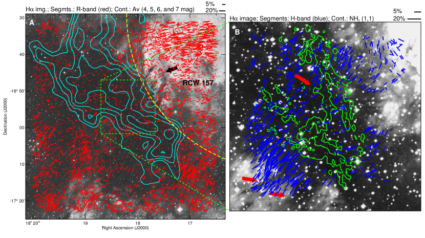
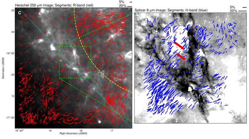
Figure 1.— Polarization maps of IRDC G14.2 showing the entire R band (a) and H band (b) datasets, as well as the foreground-corrected samples (see Section 3.2) in the R and H band (c and d, respectively). The optical mapping (red segments) covers a large-area around the cloud that is indicated by the cyan-colored $A_{V}$ contours in panel a (4, 5, 6 and 7 mag levels, Dobashi et al., 2013). The NIR dataset (blue segments) is focused on the central filamentary features (green contours in panel b, representing the integrated NH₃(1,1) emission with levels of 40 mJy beam^-1 km s^-1, from Paper I). Polarization segments lengths are scaled proportional to $\sqrt{p}$ (each panel shows reference sizes for $5\%$ and $20\%$ segments in the top right). Background images are from the SuperCOSMOS H$\alpha$ survey in panels a and b (Parker et al., 2005), from Herschel-SPIRE $250\,\mu$m in panel c and Spitzer-IRAC $8\,\mu$m in panel d. The different wavelengths reveal emission features from different ISM components, such as ionized gas, cold or warm dust. The RCW 157 area is indicated by the yellow dashed line in panels a and c. Pillars at the edge of this area are located by the black arrow (see Section 4.4). Red arrows indicate striations perpendicular to the filaments, both in the H$\alpha$ (b) and Spitzer images (d, see Section 4.1). The large-scale orientation of the cloud is indicated by the dotted cyan line in panel c ($\approx 43\arcdeg$ relative to the north celestial pole).

In this work, the analysis of the R-band and H-band polarimetric samples are distinguished by the fact that they are useful in tracing respectively the large-scale and the small-scale magnetic field structure around IRDC G14.2. More specifically, here we define small scales as the typical range of lengths of the filaments found in IRDC G14.2 ($\sim 1-3$ pc, green NH₃ contours in Figure 1b), and large scales as sizes on the order of the molecular cloud in which the filaments are embedded ($\sim 20-40\,$pc, cyan visual extinction contours – $A_{V}$ – in Figure 1a). On one hand, while the R-band detections are limited by extinction to trace only more diffuse ISM, they are distributed along a large area covering the molecular cloud’s surroundings. On the other hand, the H-band polarimetry covers only the central areas, but are less affected by extinction and therefore a large number of segments are concentrated around the filaments.

In both Figures 1a and 1b the background image corresponds to H$\alpha$ observations (Parker et al., 2005). Thus, the image shows both stellar point sources and patches of bright extended emission due to the presence of the RCW 157 Hii region, also known as Sh 2-44 (outlined by the curved yellow dashed line). The association of RCW 157 Hii region with IRDC G14.2 is not clear as there is a discrepancy in the distance of RCW 157 region ($\sim 2\,$kpc according to Avedisova & Palous 1989, and $3.7\,$kpc according to Deharveng et al. 2010 and Lockman 1989). In any case, in this work we excluded from the analysis the polarization data around RCW 157 region since the original morphology of magnetic field lines might have been distorted due to the expansion of the ionized volume. More discussion will be given in Section 4.4.

Figures 1c and 1d show the foreground-corrected polarization segments, respectively in the R and H bands. The detailed process of foreground correction is discussed in Section 3.2. Background images in this case correspond to the Herschel-SPIRE $250\,\mu$m (Figure 1c) and the Spitzer $8\,\mu$m (Figure 1d). The large-scale dust cloud, as well as the complex of filamentary structures embedded within are clearly observed in these images. The close-up view from Spitzer (Figure 1d) exhibits a better resolution view of the intricate pattern of interstellar filaments, seen in absorption against the Galactic background infrared radiation.

3.2. Visual extinction estimates and foreground polarization correction

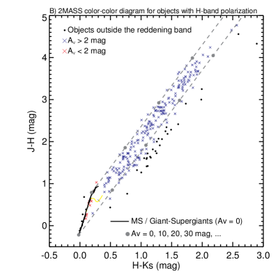
Figure 2.— Color-color $(J-H)\times(H-Ks)$ diagrams based on 2MASS for objects from the R band (a) and H band datasets (b). The loci which corresponds to the unreddened ($A_{V}=0$) main sequence, giants and supergiants, is indicated by a solid line (Koornneef, 1983; Carpenter, 2001). The reddening band (parallel to the reddening vector Fitzpatrick, 1999) is represented by dashed gray lines, in which each bullet indicated increments of 10 mag. The yellow line represents main sequence stars with spectral types later than G5.

Considering the distance to IRDC G14.2, it is likely that a considerable fraction of the detections actually correspond to foreground stars (particularly those detected in the R-band mapping). Therefore, two distinct operations must be applied to correct for the foreground contamination:

• Correction A: foreground stars must be identified at least statistically, and removed from the sample;

• Correction B: the polarization component produced by the foreground material must be determined and subtracted from the background sources.

In the general direction of the dark cloud, stars distributed along different distances probe interstellar polarization features produced by different interstellar components. Since individual distances are not known, one may use the visual extinction as a general proxy, giving us an approximate idea of the star’s location along the line-of-sight.

Estimates of the visual extinction $A_{V}$ for each stellar object were obtained based on 2MASS photometric data (Skrutskie et al., 2006). Among the total of 4627 and 584 stars from our R-band and H-band samples, respectively, 1227 and 337 were either not found in the 2MASS catalog or excluded due to poor photometry in at least one of the NIR bands ($J$, $H$ or $Ks$). Thus, the following analysis applies only to the objects found in the 2MASS catalog, with valid photometric values.

The visual extinction determination method is based on color-color diagrams $(J-H)\times(H-Ks)$ which are shown in Figures 2a and 2b for the R-band and H-band polarimetric samples, respectively. As may be noted, reddening causes points to spread along a band (gray dashed lines), since each data point is displaced from its de-reddened position an amount proportional to the visual extinction. Therefore, by de-reddening each point upon reaching the main sequence locus, it is possible to estimate $A_{V}$ by applying general interstellar relations given by Fitzpatrick (1999). This method is not meant to provide a highly precise determination of $A_{V}$, since individual spectral types are not known and general assumptions regarding the relation between color excess and extinction have to be made (Fitzpatrick, 1999). However, it is sufficiently robust to provide an approximate estimate, as needed in this work. It is important to point out that when de-reddening each point along the reddening band, the main sequence locus can be crossed twice (early-type and later-type stars), suggesting that there is an apparent degeneracy in the $A_{V}$ estimate. However, assuming the 2MASS photometric completeness limits, it is easy to show that un-reddened main sequence stars with spectral types later than G5 (the yellow line starting on the yellow plus sign) are too faint to be observed at such distances. Thus, the late-type portion of the main sequence can be ignored (the yellow line) and only the early-type main sequence locus is used, removing the ambiguity. Also notice that the early-type portion of the main sequence locus is superposed to the giants and supergiants locus in a $(J-H)\times(H-Ks)$ diagram, and thus the $A_{V}$ estimate doesn’t depend on the luminosity class. For the R-band, only objects inside the reddening band are considered valid for this calculation (red or blue crosses), while objects outside (black dots) are excluded. In this way, sources with infrared color excess (typically displaced to the right side of the reddening band), which are known to present circumstellar discs (and therefore possibly intrinsic polarization by scattering), are automatically removed.

The R-band diagram shows that there are stars with a distribution of various extinction levels. Analyzing $E(b-y)$ reddening maps from Reis et al. (2011) we notice that along the cloud’s line-of-sight, the foreground ISM closer to the Sun ($d\lesssim 300$ pc) contributes with $A_{V}\sim 1$ mag (assuming the general relation $A_{V}=4.3E(b-y)$). Estimates of the extinction and polarization levels associated to the material beyond these local regions may be done by studying the compilation of $P_{V}$ (polarization degree at the $V$ band) and $E(B-V)$ (interstellar reddening) data by Heiles (2000) as a function of distance. Considering a radius of $1\arcdeg$ centered on the cloud, 15 stars with distance smaller than $2.0$ kpc are found. Their mean R-band polarization degree and angle are respectively $0.7\pm 0.2$% and $67\arcdeg$, giving us an initial idea of the foreground polarization level. It is important to point out that we have converted the polarization degree from V to R band using the relation by Serkowski et al. (1975), assuming typical grain sizes, which corresponds to a peak in polarization spectrum around $\lambda_{max}=0.55\mu$m. The mean $E(B-V)$ value using the same 15 objects from Heiles (2000) is $0.6$ mag, corresponding to $A_{V}\approx 2.0$ mag (assuming $A_{V}=3.1E(B-V)$).

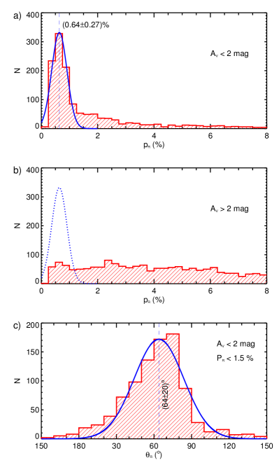
Figure 3.— Histograms used to estimate the foreground contribution to the R band polarimetric sample: panel a shows the distribution of $p_{R}$ for $A_{V}<2$ mag (which is a general proxy for the foreground extinction), with a Gaussian fit peaked at 0.64$\%$; panel b shows the distribution for $A_{V}>2$ mag (the same Gaussian fit from panel a is shown as reference); in panel c the distribution of $\theta_{R}$ is shown, considering only polarization detections with $A_{V}<2$ mag and $p_{R}<1.5\%$. The Gaussian fit indicates an average foreground polarization orientation of $\approx 64\arcdeg$.

Using the $2$ mag level as a general proxy for the foreground visual extinction, we proceed with the analysis by constructing the histograms in Figure 3. The first histogram (Figure 3a) shows the distribution of polarization values for stars with $A_{V}<2$ mag, while Figure 3b shows the distribution for $A_{V}>2$ mag. A peak is seen in the first case (the blue Gaussian fit), while for higher extinctions (Figure 3b) the Gaussian profile vanishes, shifting to a flat-like distribution. This indicates that objects encompassed by the Gaussian curve are probably foreground objects, while higher extinction sources are most likely background stars. To determine the foreground polarization angle, the third histogram (Figure 3c) shows $\theta_{R}$ for stars with $A_{V}<2$ mag and $p<1.5\%$ (i.e., considering only objects below the Gaussian curve of Figure 3a). From the peak of Gaussian fits of Figures 3a and c, we estimate values of respectively 0.67% and $64\arcdeg$ for polarization percentage and orientation angle in the R band, matching very well the expectations based solely on the Heiles (2000) data. Additionally, the foreground value obtained is practically invariant under slight changes in the $A_{V}$ and $p$ cut-offs used here, showing that this is a robust computation.

Notice that the shape of the polarization angle distribution in Figure 3c deviates slightly from a Gaussian-like, suggesting that the foreground component is not perfectly uniform across the field. This is not unexpected, given the wide field-of-view of the R-band survey area. The non-uniformity probably corresponds to a smooth change in the foreground polarization angle across the field, since the distribution shows a unique non-symmetrical wide peak instead of multiple peaks clearly distinguishable. Even though in this work we are adopting a single average foreground component, it is relevant to point out that for the purposes of the removal of this component from background sources (Correction B), the analysis that will be presented in Section 3.3 is very robust, and the same results are obtained even if no subtraction is applied (although Correction A is still important). The main reason is that the foreground component is usually small compared to polarization levels of background stars, for which the molecular cloud component is predominant.

To apply Correction A, in order to be conservative in the selection of background sources, we consider only those with $A_{V}>2$ mag and $p>2.0\%$ (i.e., those outside the range of the Gaussian fit from Figure 3a), and we also exclude sources not found in 2MASS or rejected due to poor photometry. For Correction B, we first calculate the mean foreground Q and U Stokes parameters using the mean foreground polarization that was previously obtained ($p_{V}=0.67\%$ and $\theta_{V}=64\arcdeg$). Then, we subtract this mean foreground Q and U value from each background star, finally determining a sample of foreground-corrected R-band detections which are probably mostly composed of background sources. The polarization segments for the foreground-corrected sample is shown in Figure 1c.

In the case of the H-band sample, the color-color diagram (Figure 2b) shows that only a few stars are low extinction sources ($A_{V}<2$ mag). These few objects are excluded from the final sample, lending the map from Figure 1d, in which most sources are probably from the background, given their $A_{V}$ levels. The small fraction of foreground stars found in the H-band dataset with 2MASS data suggests that even considering the entire dataset (including objects not found in 2MASS or excluded due to poor photometry), the vast majority of stars are probably background sources. Thus, we consider objects not found in 2MASS (or rejected) as background sources for the H-band polarization analysis in this work. For subtraction of the foreground component from background sources (Correction B), we find that in the H band the contribution is negligible: if $p=0.67\%$ in the R band, then assuming the Serkowski relation, the H-band foreground polarization would be approximately 0.15%. Since this is a small level of polarization, lower than the typical uncertainty in polarization degree, we choose to ignore its contribution. This avoids introducing unnecessary systematic uncertainties, since the estimate of $0.15\%$ for the H-band foreground polarization (extrapolating from the R band) involves assumptions regarding the peak of the polarization spectral function.

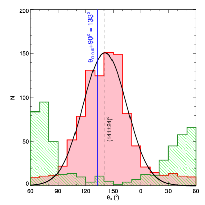
Figure 4.— Histogram (red) of the foreground-corrected orientation of polarization segments in the R-band (as shown in Figure 1c), excluding the RCW 157 region. The peak of the distribution ($\approx 141\arcdeg$) is found through the Gaussian fit, being approximately perpendicular to the large-scale cloud orientation ($\theta_{\mathrm{cloud}}+90\arcdeg=133\arcdeg$). The green histogram correspond to foreground objects removed from the sample (see Correction A in Section 3.2).

3.3. Relation between polarization segments and the large-scale cloud orientation

After removal of the foreground stars from the R-band sample, it is possible to investigate the relation between the orientation of polarization segments and the large-scale cloud in which the interstellar filaments are embedded. This may help determine the range of spatial scales in which magnetic fields might be important in regulating the gravitational collapse.

Figure 4 shows a histogram of R-band polarization angles (red), excluding the area defined by the RCW 157 Hii region (above the dashed yellow line in Figure 1a). Although there is a large dispersion, a peak around $141\arcdeg$ is clearly identified (as shown by the Gaussian fit). In comparison, the direction perpendicular to the cloud ($\theta_{\mathrm{cloud}}+90\arcdeg$) is indicated by the blue line, as $\sim 133\arcdeg$ (the cloud’s direction, $\approx 43\arcdeg$, is shown by the cyan-colored dotted line in Figure 1c). It is clear that there is an overall correlation between the large-scale magnetic field lines and the direction perpendicular to the cloud.

It is important to point out that, particularly for this analysis, the previous removal of foreground sources was essential (Correction A), since these comprised a considerable fraction of the vector sample. The green histogram in Figure 4 shows foreground stars that were removed from the sample. Notice that foreground segments in general are parallel to the cloud, which is an opposite trend compared to background sources. Comparing Figures 1a and c, it is straightforward to visualize the sample of foreground stars that has been removed (which are mostly low polarization detections parallel to the cloud orientation). Therefore, if not previously removed, this component would have introduced considerable contamination in this analysis, impairing the notion that on-site magnetic field lines in general are perpendicular to the large-scale cloud.

3.4. Relation between polarization segments and the orientation of filaments

Figure 5a shows the H-band polarization segments superposed to the Spitzer $8\,\mu$m image, together with the location of filaments represented by colored straight lines. In Paper I, these structures were distinguished between hubs and filaments depending on physical features obtained from the NH₃ observations: hubs were classified as structures presenting signs of star formation, as well as higher rotational temperatures and non-thermal velocity dispersions ($T_{\mathrm{rot}}\sim 15\,$K and $\sigma_{\mathrm{NT}}\sim 1\,$km s^-1) as compared to filaments ($T_{\mathrm{rot}}\sim 11\,$K and $\sigma_{\mathrm{NT}}\sim 0.6\,$km s^-1).

Figure 5b shows a histogram of polarization orientation in the H band ($\theta_{H}$), which includes all the detections shown in Figure 5a. It clearly exhibits a peak at $\theta_{H}=139\arcdeg$. It is interesting to note that the main orientation at such smaller scales matches very well the average orientation at large-scale (from the Figure 4).

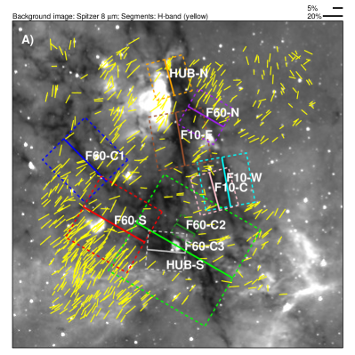
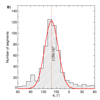
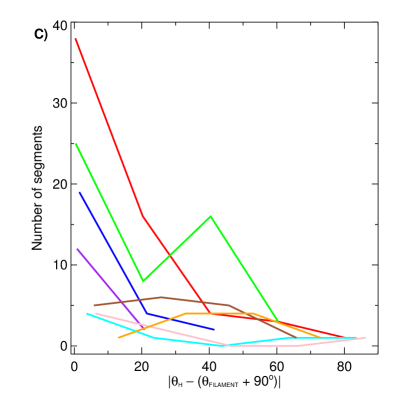
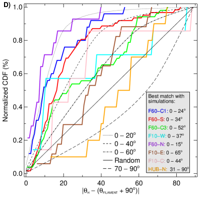
Figure 5.— Analysis of the relative orientation between H band polarization segments and interstellar filaments. Panel a shows the Spitzer $8\mu$m image with the polarimetric data (same as Figure 1d), as well as dashed colored boxes with sizes equal to each filament’s length (represented by the solid lines, as defined in Paper I). Panel b shows the histogram of polarization orientation for all H-band detections in the field. Panels c and d respectively show the regular histograms and cumulative distribution functions (CDFs) of the difference between polarization angle and the orientation perpendicular to each filament, considering only the segments within the boxes (the colors match each box in panel a). Black lines shows numerical predictions for the CDFs, as based on Monte Carlo simulations. Preferential ranges for tridimensional angle differences of $\Delta a=0-20\arcdeg$, $0-40\arcdeg$, $0-60\arcdeg$ and $70-90\arcdeg$ are indicated as reference, as well as a completely random distribution (the solid line). The best $\Delta a$ match with the simulations for each filament are listed in the gray box.

The relative orientations of segments and filaments are projected into the plane of the sky, so the true relative orientations are unknown. To carry out a quantitative analysis of the relative orientations, a box was drawn around each filament, with sizes matching the length of each structure (from Paper I). Thereafter, segments inside each box were selected in order to represent the orientation of magnetic field lines in the immediate surroundings of each filament. For each vector, its orientation relative to its corresponding filament’s perpendicular direction was computed ($|\theta_{H}-(\theta_{\mathrm{filament}}+90\arcdeg)|$).

Figures 5c and 5d respectively show the regular distributions and the Cumulative Distribution Functions (CDFs), using the relative orientations of segments for each filament (Hub-S and F60-C2 were omitted). The histograms and CDFs are shown with colored lines that match each respective filament (and its box). Although there is considerable variation in the orientation of polarization segments throughout the field, there is a clear trend for an overall orientation perpendicular to the filaments. This can be seen by the peaks close to zero for some of the histograms in Figure 5c.

In order to account for the possible geometrical projection effects, we compared the CDFs to Monte Carlo simulations of a set of relative projected angles based on a large number of vector-filament pairs randomly distributed in tridimensional space. For each individual simulation, we selected only pairs in which the true relative orientation was within a certain range of values (denoted by $\Delta a$). Using this subset of segments, we projected the pairs in the plane of the sky and then computed the CDF of the projected relative orientations. Examples for $\Delta a$ equal to $0-20\arcdeg$, $0-40\arcdeg$, $0-60\arcdeg$, and $70-90\arcdeg$ are shown in Figure 5d, as well as the random condition (or $0-90\arcdeg$).

To find out which $\Delta a$ configuration from the simulations would best represent the segments’ orientations for each filament, we begin by running it for all possible $\Delta a$ ranges. Then, for each filament, we compare its observed CDF to each of the various simulated CDFs through Kolmogorov-Smirnov tests, which are useful to verify the statistical probability of two different distributions be drawn from the same ensemble. Finally, the comparison which provided the larger probability was chosen as the best simulation that could represent the observed CDF. The $\Delta a$ for the best representative simulation for each filament is shown in Figure 5d.

As expected by visual inspection, the majority of the filaments present $\Delta a$ upper limits significantly lower than $90\arcdeg$. This means that there is a very clear trend of filaments and hubs being perpendicular to magnetic field lines, even when considering that both the filaments and the polarization segments orientations represent a projection in the plane of the sky. There are, however, some situations where the statistics is not ideal (for example, the small number of detections for F10-C and F10-W) and a few exceptions, for example: for Hub-N, the best representative simulation corresponds to a $\Delta a$ range between $31$ and $90\arcdeg$, suggesting a slight trend of magnetic field lines parallel to the hub. In addition, the distribution for F10-E is only marginally representative of a perpendicular condition. It is interesting to notice that these discrepancies occur exactly for the two structures that are spatially closer to IRAS 18153-1651, the bright ultra-compact Hii region to the east of Hub-N and F10-E. This suggests that magnetic field lines in these structures might have been disrupted by the Hii region expansion. Further discussion is given in Section 4.1.

3.5. Statistical derivation of the magnetic field strength

In order to understand the interplay between magnetic field support, gravity and turbulence for each filamentary structure, important physical parameters may be calculated by combining the H-band polarization data with velocity dispersion data from molecular-line studies and density information. These parameters are the plane-of-the-sky component of the magnetic field strength ($B_{\mathrm{pos}}$), the Alfvén Mach number ($M_{A}$) and the mass-to-magnetic-flux ratio ($\lambda$).

Given a set of polarization segments surrounding a certain filament or hub, the Chandrasekhar-Fermi (CF) theory (Chandrasekhar & Fermi, 1953) states that the magnetic field strength in that volume of the ISM is inversely proportional to the angular dispersion of polarization segments, a quantity that is related to turbulence. A quantitative method may be applied to study such angular dispersion factor, which represents the signature of interstellar turbulent motion impinged in the morphology of magnetic field lines in that area. The method consists in a statistical analysis, proposed first by Hildebrand et al. (2009) and extended later on by Houde et al. (2009), which takes into account the effect of the line-of-sight depolarization. This method has been successfully applied to optical polarization data (Franco et al., 2010) as well as to submillimeter polarization data (e.g., Houde et al., 2011; Girart et al., 2013; Frau et al., 2014).

As shown by Houde et al. (2009) the angular dispersion function (ADF) can be used to estimate the importance of the magnetic field. We have estimated the angular dispersion function, $1-\langle\mathrm{cos}[\Delta\Phi(l)]\rangle$, where $\Delta\Phi(l)$ is the difference in polarization angles between two points in the plane of the sky separated by a distance $l$. The analysis is based on the assumption of a stationary, homogenous, and isotropic magnetic field strength and a magnetic field turbulent correlation length, $\delta$, smaller than the thickness of the cloud $\Delta^{\prime}$. Under these assumptions, the angular dispersion function (Equation (42) from Houde et al. 2009) can be expressed as

$$1-\langle\,\mathrm{cos}[\Delta\Phi(l)]\rangle \simeq \frac{\langle\,B_{\mathrm{t}}^{2}\rangle}{\langle\,B_{\mathrm{0}}^{2}\rangle}\frac{1}{N}[1-e^{l^{2}/2(\delta^{2}+2W^{2})}]$$ (1)

$$+\sum_{j=1}^{\infty}\,a_{2j}^{{}^{\prime}}l^{2j},$$

where $l$ is the length scale, $W$ is the standard deviation of the Gaussian beam ($W=FWHM/\sqrt{8\,\mathrm{ln}\,2}$), $\delta$ is the turbulent correlation length, and $N$ is the number of independent turbulent cells along the line of sight,

$$N=\biggl{[}\frac{(\delta^{2}+2W^{2})\Delta^{\prime}}{\sqrt{2\pi}\delta^{3}}\biggr{]}.$$ (2)

The summation term represents the contribution from the ordered component of the magnetic field that does not involve turbulence. The coefficient $a_{2j}$ represents to the steepness of the function in this ordered component. For stellar polarimetry data, the beam size can be considered as a pencil beam, since $W$ is negligible relative to the turbulent length scale $\delta$ (thus $W$ may be ignored). The intercept of the fit to the data of the uncorrelated part at $l=0$, $f_{\mathrm{NC}}(0)$, allows us to estimate the turbulent to large-scale magnetic field energy ratio ($\langle\,B_{\mathrm{t}}^{2}\rangle/\langle\,B_{\mathrm{0}}^{2}\rangle$) as

$$\frac{\langle\,B_{\mathrm{t}}^{2}\rangle}{\langle\,B_{\mathrm{0}}^{2}\rangle}=N f_{\mathrm{NC}}(0).$$ (3)

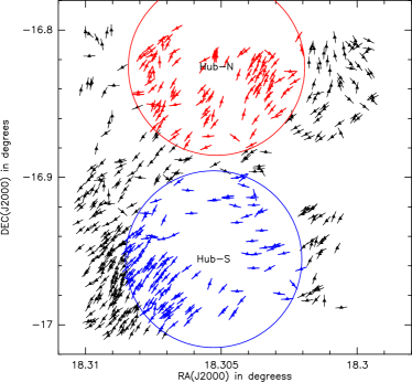
Figure 6.— Magnetic field direction obtained from H-band polarization data in IRDC G14.2. Red and blue segments indicate the polarization data used to compute the angular dispersion function around Hub-N and Hub-S, respectively.

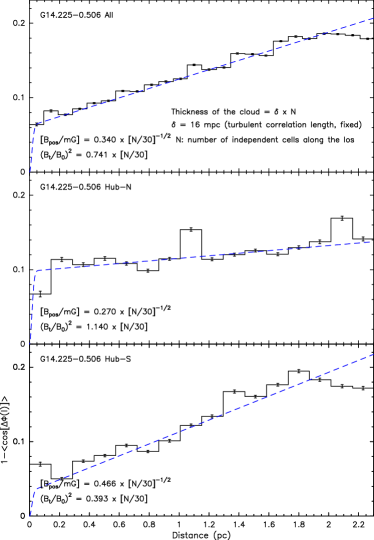
Figure 7.— Angular dispersion function of the magnetic field segments detected toward the IRDC G14.2 considering all B-field segments (top), Hub-N (middle), and Hub-S (bottom) considering, respectively, the red and blue B-field segments shown in Fig. 6. The data points and error bars are the mean and standard deviation of all the pairs contained in each bin. The blue dashed line shows the best fit to the data (Equation 1).

The low statistics obtained in the IRDC G14.2 prevent us to conduct the statistical analysis to fit the ADF for each filament and hub individually. Instead, to analyze the magnetic field, we considered three different regions: all the cloud, and the two hub-filament systems identified in Paper I, Hub-N and Hub-S. We defined a radius, $R=0.06\arcdeg$ or $\sim 2$ pc, from the center of each hub (Busquet et al., 2013, 2016) to estimate the angular dispersion function for all the measurements that are at a distance $<R$ of the hub. Figure 6 shows the circles centered in each hub for this radius, indicating the polarization values used to compute the ADF for Hub-N (in red) and Hub-S (in blue). The radius of $0.06\arcdeg$ was chosen using the following criteria: (1) to make sure sufficiently wide areas around Hubs N and S were covered, while also avoiding an overlap between them; (2) to avoid including in the Hub-N area a group of polarization segments to the right of the red circle that clearly show a different mean orientation, probably related to the edge of RCW 157 (compare with Figures 1a and b). In Figure 7 we present the angular dispersion function for all the cloud (top panel), Hub-N (middle panel), and Hub-S (bottom panel). One may notice that each function consists of a gradual rise starting from $l=0$, which may be interpreted as a decrease in the correlation of polarization orientation for segments separated by increasingly larger angular distances. The behavior of the ADF is slightly different in the two regions defined around each hub, with Hub-N having a more flattened slope than Hub-S, indicating that the large-scale magnetic field in the plane of the sky is quite uniform. The best fit of Eq. 1 to the polarimetric data is shown in Fig. 7 with the blue dashed line.

To calculate $\langle\,B_{\mathrm{t}}^{2}\rangle/\langle\,B_{\mathrm{0}}^{2}\rangle$, we begin by estimating $N$, which is related to the cloud thickness along the line of sight $\Delta^{\prime}=\sqrt{2\pi}\,N\delta$ (see equation 2). In other star forming regions, the turbulent correlation length $\delta$ was found to be equal to $16$ mpc (OMC-1, Houde et al. 2009; DR21-OH, Girart et al. 2013), or varying between $13$ and $33$ mpc in NGC7538 IRS1 (Frau et al., 2014). Based on these previous estimates, in this work we fix $\delta=16$ mpc since it is not the main source of uncertainty, as will be noted below.

The cloud thickness can be estimated by taking the ratio between the column density $N_{\mathrm{H_{2}}}$ and the volume density $n(\mathrm{H_{2}})$. We should point out that both quantities are estimated here for the material surrounding the filaments, to coincide with the region where the H-band polarization data is distributed. The volume density is the main source of uncertainty for this calculation, so the approach is to find reasonable lower and upper limits around the filaments, and use this range as a proxy to determine the uncertainty in the magnetic field strength. For the lower limit, we notice that the C¹⁸O (1-0) line data from IRAM 30m (Busquet et al. in prep.) reveals an emission present over the entire IRDC G14.2 field, covering not only the dense filaments but also their surroundings. Thus, a conservative estimate for the lower limit is the critical density of C¹⁸O (1-0) which is $\sim 1.4\times 10^{3}$ cm^-3 (Myers, 1999). From the same molecular line survey, we find that the HCN (1–0) line is also detected in the more diffuse area between filaments, thus its effective excitation density $4.5\times 10^{3}$ cm^-3 (assuming a temperature of $20$ K, see Table 1 of Shirley 2015), is representative of the typical density in this material. For the upper limit, we know that the density cannot be too much higher than $10^{4}$ cm^-3, because molecular line transitions with higher excitation densities (such as the HC₃N (10–9) line, with and excitation density of $4.3\times 10^{4}$ cm^-3 at $20$ K) are found in emission only toward the densest portions of the filaments. Therefore, we adopt the range of $n(\mathrm{H_{2}})$ between $\sim 1.4\times 10^{3}$ cm^-3 and $10^{4}$ cm^-3, and propagate the uncertainties into the cloud thickness, $\langle\,B_{\mathrm{t}}^{2}\rangle/\langle\,B_{\mathrm{0}}^{2}\rangle$, and the magnetic field strength.

The column density ($N_{\mathrm{H_{2}}}$) can be estimated for the inter-filament region by two independent methods: (1) Using multi­wavelength dust emission maps (from ground-based – CSO, APEX – and space telescopes – Herschel, Planck) to carry out a single component, modified black-body fit to each pixel of the maps (Lin et al. 2016, in prep.). The derived values for the region sampled by NIR polarization are typically $T\approx 20$ K and $N_{\mathrm{H_{2}}}\approx 10^{22}$ cm^-2; (2) Using the RADEX on-line one-dimensional non-LTE radiative transfer code (van der Tak et al., 2007) to obtain the column density based on the C¹⁸O (1-0) line. As inputs to the line data model, we used a line width of $\sim 2$ km s^-1, temperatures of $20$ K and volume densities in the range of $\sim 1.4\times 10^{3}$ cm^-3 to $10^{4}$ cm^-3. These inputs result in C¹⁸O column densities between $2\times 10^{22}$ cm^-2 and $5\times 10^{22}$ cm^-2. Assuming the standard ¹⁶O/¹⁸O ratio for the local ISM of 560 (Wilson & Rood, 1994), and adopting the standard abundance of CO with respect to H₂ of $10^{-4}$, we find $H_{2}$ column densities in the range $1-2\times 10^{22}$ cm^-2. Therefore, $N_{\mathrm{H_{2}}}$ is well constrained by two independent methods to be $\approx 10^{22}$ cm^-2, and we adopt this as a fixed value to obtain the cloud thickness. The range of cloud thickness is between $0.32$ and $2.31$ pc, yielding a number of independent cells ranging from $N=10$ to $60$. Using an average value of $N=35$, this implies that $\langle\,B_{\mathrm{t}}^{2}\rangle/\langle\,B_{\mathrm{0}}^{2}\rangle$ in all the cloud is 0.86, while the values are 1.33 and 0.46 in Hub-N and Hub-S, respectively (see Table 1, which also shows the uncertainties). Note that around Hub-N there is equipartition between the perturbed (turbulent) and ordered magnetic field energies whereas around Hub-S uniform magnetic field dominates energetically over turbulence.

Finally, the CF equation can be used to derive the plane-of-sky magnetic field strength for each region (Equation (57) of Houde et al. 2009):

$$\langle\,B_{\mathrm{0}}^{2}\rangle^{1/2}\propto\,\sigma_{v}\,n(\mathrm{H_{2}})^{1/2}[\langle\,B_{\mathrm{t}}^{2}\rangle/\langle\,B_{\mathrm{0}}^{2}\rangle]^{-1/2},$$ (4)

where $\sigma_{v}$ is the velocity dispersion and $n$(H₂) the volume density. The velocity dispersion was obtained from the C¹⁸O (1–0) data (Busquet et al. in prep.) that traces the diffuse gas around the dense filaments and hubs, resulting in $\sim 2$ km s^-1. It is important to point out that for the CF method, the relevant velocity dispersion component is the one generated by turbulence in the ISM. For molecular clouds, the thermal velocity dispersions are typically much smaller than the non-thermal velocity dispersions, so it is reasonable to assume that $\sigma_{v}=\sigma_{v(\mathrm{NT})}+\sigma_{v(\mathrm{thermal})}\approx\sigma_{v(\mathrm{NT})}$. Moreover, the non-thermal velocity dispersion component can be produced by turbulent motions, gravitational infall, or rotation. Although numerous star-forming regions present signatures of infall even at larger scales (Peretto et al., 2013, 2014; Duarte-Cabral et al., 2014; Henshaw et al., 2014; Liu et al., 2015; Campbell et al., 2016; Wyrowski et al., 2016), it is unclear whether it would cause a significant effect in the observed line-widths in comparison with turbulence, specially in the diffuse regions around filaments. In this work, we assume that the velocity dispersion derived from the C¹⁸O (1–0) data is mostly due to turbulent motions, but this is a matter that will require further investigation.

The ordered large-scale magnetic field strength component in the plane of the sky, $\langle\,B_{\mathrm{0}}^{2}\rangle^{1/2}$, for each defined region is listed in Table 1, where the uncertainties are derived from the range of volume densities $n$(H₂). Considering the entire set of H-band polarization data associated with IRDC G14.2 the sky-projected magnetic field strength component is 0.39 mG, while for Hub-N and Hub-S they are given by $\sim$0.32 and 0.55 mG, respectively.

It is important to point out that if the total magnetic field $B_{\mathrm{tot}}$ has an inclination $\beta\neq 90\arcdeg$ with respect to the line-of-sight, then the CF calculation will lead to underestimated values, since what is being measured is only the plane-of-sky component: $B_{\mathrm{pos}}=B_{\mathrm{tot}}\sin{\beta}$. The inclination $\beta$ is unknown and therefore it is difficult to correct for this effect in a precise way. However, Crutcher et al. (2004) showed that it is possible to account for it at least statistically by integrating over all possible $\beta$ values. That leads to the following correction which is being applied here: $B_{\mathrm{tot}}=(4/\pi)B_{\mathrm{pos}}$. Table 1 lists the values for the total magnetic field values computed for each region, with its respective uncertainties.

Table 1 Physical properties in IRDC G14.2

Region	$\langle\,B_{\mathrm{t}}^{2}\rangle/\langle\,B_{\mathrm{0}}^{2}\rangle$	$B_{\mathrm{pos}}$ (mG)	$B_{\mathrm{tot}}$ (mG)	$M\,(\mathrm{M}_{\odot}$)	$N_{\mathrm{H_{2}}}$ (cm-2)	$\lambda$	$M_{A}$
Cloud	$0.86\pm 0.62$	$0.31^{+0.28}_{-0.07}$	$0.39^{+0.36}_{-0.09}$	4660	$2.8\times 10^{22}$	0.6	0.7
Hub-N	$1.33\pm 0.95$	$0.25^{+0.22}_{-0.06}$	$0.32^{+0.28}_{-0.08}$	2000	$4.5\times 10^{22}$	1.1	0.8
Hub-S	$0.46\pm 0.33$	$0.43^{+0.38}_{-0.10}$	$0.55^{+0.48}_{-0.13}$	1550	$3.5\times 10^{22}$	0.5	0.5

3.6. Estimates of mass-to-magnetic-flux ratios and Alfvén Mach numbers

To understand if magnetic fields are strong enough to support clouds against gravitational collapse, it is useful to study the mass-to-magnetic-flux ratio ($M/\Phi$) which is conveniently calculated relative to a critical value given by $(M/\Phi)_{\mathrm{crit}}=1/2\pi\sqrt{G}$ (Nakano & Nakamura, 1978), where $G$ is the gravitational constant and $\Phi$ is the magnetic flux. Crutcher et al. (2004) showed that this relative quantity may be expressed as a function of the $\mathrm{H_{2}}$ column density ($N_{\mathrm{H_{2}}}$) and the total magnetic field strength:

$$\lambda=\frac{(M/\Phi)}{(M/\Phi)_{\mathrm{crit}}}=7.6\times 10^{-21}\Big{(}\frac{N_{\mathrm{H_{2}}}}{\mathrm{cm}^{-2}}\Big{)}\Big{(}\frac{B_{\mathrm{tot}}}{\mu\mathrm{G}}\Big{)}^{-1}$$ (5)

It is known that $\lambda$ can be affected by the geometry of the cloud (Crutcher et al., 2004). However, given the intricate arrangement of filamentary features at the IRDC G14.2 region, we chose not to make any assumptions regarding its morphology.

Furthermore, in order to access the importance of the interstellar turbulent motion in disturbing the magnetic field lines, we calculate the Alfvén Mach number, which is given by:

$$M_{\mathrm{A}}=\frac{\sqrt{3}\,\sigma_{v}}{V_{A}}$$ (6)

where $V_{A}=B_{\mathrm{tot}}/\sqrt{4\pi\rho}$ is the Alfvén speed. $M_{\mathrm{A}}$ can be viewed as a measure of the ratio between the turbulent and magnetic energies (in fact, this ratio is given by $M_{\mathrm{A}}^{2}$), and therefore the sub-alfvénic ($M_{\mathrm{A}}<1$) or super-alfvénic ($M_{\mathrm{A}}>1$) conditions indicate whether the relative importance of magnetic field support against the gravitational collapse is higher or lower as compared to turbulence in the ISM. Notice that similarly to the CF method, we assume that the non-thermal motions are dominated by turbulence.

To obtain the mass and column density of each defined region we integrate the dust continuum emission at 870 $\mu$m (Busquet, 2010) over the same area where $B_{\mathrm{pos}}$ is measured. Notice that this integration also includes the dense structures within the selected areas, since the goal of calculating $\lambda$ is to evaluate the gravitational stability of the cloud against magnetic field support. In cold and dense clouds like IRDCs dust grains are supposed to be coagulated and covered of icy mantles (Peretto & Fuller, 2009), so we derived the mass by adopting a dust mass opacity coefficient at 870 $\mu$m of 1.7 cm² g^-1, which corresponds to agglomerated grains with thick ice mantles in cores of densities $\sim 10^{5}$ cm^-3 (Ossenkopf & Henning, 1994), and assuming that the dust emission at 870 $\mu$m is optically thin, a gas-to-dust ratio of 100, and a dust temperature of 17 K. Dust temperature has been obtained using the rotational temperature derived from NH₃ data of Paper I and converted to kinetic temperature though the prescription adopted by Tafalla et al. (2004). For the column density, $N(\mathrm{H}_{2})=M/\mu\,m_{\mathrm{H}}A$, where $\mu=2.8$ is the molecular weight per hydrogen molecule, $m_{\mathrm{H}}$ is the mass of the hydrogen, and $A$ is the area used to derive the mass. The final values of $M$, $N(\mathrm{H_{2}})$, $\lambda$, and $M_{\mathrm{A}}$ are reported in Table 1. As with the magnetic field values, the uncertainties in $\lambda$ and $M_{\mathrm{A}}$ can reach around a factor of 2. Similar values of $M_{\mathrm{A}}$ and $\lambda$ are found by Pillai et al. (2015) toward two massive IRDCs using submillimeter polarization data.

4. Discussion

4.1. Cloud and filament formation through gravitational collapse parallel to magnetic field lines

The polarization data from large to small scales at the IRDC G14.2 region show that not only magnetic fields are tightly perpendicular to the star-forming dense filamentary structures within (with a few exceptions, as discussed below), but also the cloud as a whole (in which the filaments constitute the densest parts at the center) has a long-shaped morphology perpendicular to the local magnetic field lines. This suggests a scenario in which magnetic fields have played an important role in regulating the gravitational collapse, being dynamically important in shaping elongated ISM structures from size scales of $\sim 30$ pc down to $\sim 2$ pc.

It is obvious from Figure 4 that there is a large dispersion in the relative orientation between the R-band segments and the cloud. This is not surprising, given that there are numerous hierarchical substructures and diffuse filamentary features around the entire region, as shown by the Herschel image (Figure 1c). Some coupling between the magnetic field lines and these diffuse clouds are expected, which may explain a fraction of the dispersion observed. However, the general trend of magnetic fields perpendicular to the cloud is still evident.

At smaller scales ($\sim 2\,$pc), the analysis on Figure 5 shows that filaments and hubs are remarkably well oriented perpendicularly to magnetic field lines. It is interesting to see that field lines show some smooth variations in orientation inside this area, and the orientation of filaments seem to follow these smooth variations. This is a further indication that magnetic fields favored the gravitational collapse of these structures parallel to field lines.

Two important exceptions are: Hub-N, which exhibits a slight trend of magnetic field lines parallel to the structure; and F10-E, which shows only a marginal perpendicular correlation with the filament axis. It is possible that the original field morphology in this area has been disrupted due to its proximity with IRAS 18153-1651, an ultra-compact Hii region seen in the Spitzer $8\,\mu$m image as a bright extended area right next to Hub-N (Figure 5a). Paper I showed that this hub has likely been heated by the interaction with the ultra-compact Hii region, and its NH₃ velocity is consistent with an expanding shell. This is consistent with the fact that the turbulent-to-uniform magnetic field energy ratio ($\langle\,B_{\mathrm{t}}^{2}\rangle/\langle\,B_{\mathrm{0}}^{2}\rangle$) is higher in Hub-N, compared to Hub-S and the entire cloud.

Recent observations show that the presence of magnetic fields aligned perpendicularly to filaments seems to be an ubiquitous characteristic of star-forming clouds (e.g., Franco et al., 2010; Li et al., 2013; Zhang et al., 2014), at least when considering densities above a certain threshold. The most recent evidence comes from the all-sky polarimetic observations of the Planck space telescope: by analysing a group of nearby molecular clouds, Planck Collaboration et al. (2016) showed that the relative orientations studied as a function of column density gradually changes from preferentially parallel or random to preferentially perpendicular. Furthermore, previous works by Goldsmith et al. (2008) and Tassis et al. (2009) also showed that within dense environments, magnetic fields are most likely perpendicular to the main filamentary structures, perhaps even being responsible for channeling interstellar material through diffuse striated features also perpendicular to the filaments. More recently, Zhang et al. (2014) surveyed a sample of 14 massive star forming clumps and filaments at 870 $\mu$m using the polarimeter on the Submillimeter Array. By comparing the dust polarization at dense core scales of $0.01-0.1$ pc with the pc-scale polarization, they concluded that magnetic fields play an important role in channeling gas during the collapse of the clump and the formation of dense cores. Therefore, magnetic fields appear to be dynamically important even at scales smaller than 1 pc.

Particularly in IRDC G14.2, Paper I pointed out that some striations are seen in the NH₃ map, converging towards filament F10-E. A visual inspection of the H-band polarization map shows that segments superposed to the striations are parallel to them, and perpendicular to the main filament, suggesting flows of material possibly converging into the main filament are parallel to magnetic fields (red arrows in Figures 1b and 1d). Some striations parallel to polarization segments may also be seen after a close visual inspection of the H$\alpha$ image (Figure 1b, red arrows along its bottom-left portion), identified as dark patches observed against a bright extended emission. This suggests a scenario similar to the ones observed in the Taurus molecular cloud (Goldsmith et al., 2008), in the Riegel-Crutcher cloud (McClure-Griffiths et al., 2006), and in Lupus I (Franco & Alves, 2015). However, in these three examples, the interstellar structures were nearby, which allowed a clearer view of the diffuse striations.

It is instructive to point out that an alternate explanation for the perpendicular condition between filaments and magnetic field lines could be proposed: the same configuration would be expected if magnetic field lines were dragged inwards by infalling material, which could also produce the striations previously mentioned. However, it is difficult to reconcile this scenario with the fact that magnetic fields at large-scales are also perpendicular to the filamentary features inside the cloud. In addition, the magnetically dominated gravitational collapse scenario is supported by MHD simulations, as described in Section 4.2.

4.2. Comparison with simulations and analysis of stability against magnetic field support and turbulent motions

Recently, Van Loo et al. (2014) developed numerical simulations designed to model the non-linear evolution of a gravitational instability within a layer of interstellar material threaded by magnetic fields. The simulations show that although the presence of magnetic fields doesn’t seem to influence on settling the filaments’ central density profiles (which is more consistent with a typical hydrodynamical equilibrium structure), they play an important role in determining their morphological and spatial distribution. While weak magnetic fields lead to spiderweb-like filamentary features, strong magnetic fields often generate a network of parallel filaments aligned perpendicular to field lines.

Given the similarities of the model outcomes with the morphological features of IRDC G14.2, Van Loo et al. (2014) compared their simulations with a fraction of the IRDC G14.2 area (specifically around Hub-N) using the polarimetric data from this work that was available at that time in Paper I. They find that the formation of these filaments is consistent with fragmentations of a layer threaded with strong magnetic fields, leading to parallel elongated structures perpendicular to field lines. The polarimetric observations from the present work provides further support for this model, and generalizes its conclusions for the entire filamentary network of IRDC G14.2. The high magnetic field strengths estimated here ($\approx 320-550~{}\mu$G) support a scenario in which the initial conditions favored a collapse of density perturbations parallel to magnetic fields, leading to the morphology of parallel filaments currently observed. Van Loo et al. (2014) estimated that for IRDC G14.2, the magnetic field values would need to be stronger than $12-25~{}\mu$G in their “strong magnetic field” model, in which parallel filaments are expected to be formed. Our estimated values are one order of magnitude higher than this lower limit, showing that IRDC G14.2 is well into the strong magnetic field regime.

Alfvén Mach numbers ($M_{\mathrm{A}}$) calculated for each defined region show that the sub-alfvénic condition is pervasive at these small scales, implying that the magnetic field strength dominates over the turbulent motion. Furthermore, the values of $\lambda$ are in the range $0.5-1.1$, suggesting a sub-critical condition (although they are close to the critical value, especially considering that there is an uncertainty in the cloud’s thickness). However, active star formation is already taking place (Wang et al., 2006; Povich & Whitney, 2010), suggesting that although magnetic fields seem to be strong enough to dominate over turbulence, it was usually not sufficient to prevent the gravitational collapse, which eventually led to star formation. Therefore the close-to-critical condition might be related to the filaments’ envelopes, while the denser interior (not probed by the polarization data) has probably reached supercritical conditions. $\lambda$ values may depend on whether the envelopes or the cores are probed (Bertram et al., 2012).

4.3. Magnetic fields related to the evolutionary sequence of the IRDC G14.2 complex

Using single-dish ¹²CO observations, Elmegreen & Lada (1976) provided the first description of the molecular cloud in which IRDC G14.2 is located, dividing the region into four fragments named A-D. Fragment C is roughly coincident with the position of IRDC G14.2. According to Elmegreen & Lada (1976), these fragments seem to be part of an evolutionary sequence: nearby star-forming region M17, together with fragments A and B, are somewhat more evolved, while fragments C and D appear to be younger.

Using the densities and velocity dispersions from the ¹²CO data, Elmegreen & Lada (1976) estimated that the fragments appear to be contracting on a time scale which is 2-3 times larger than the free-fall time, suggesting that strong internal magnetic fields of $\sim 340\,\mu$G could be providing some support against the collapse in fragment C. Their estimate, which is based on equipartition is remarkably similar to the values of magnetic field strengths computed in this work for the filamentary structures within IRDC G14.2. However, it is important to point out that interstellar structures with larger aspect ratios (such as filamentary features) have longer collapse timescales as compared to spherical clouds (Pon et al., 2012). Thus, an alternative explanation for the 2-3 times discrepancy in contraction time observed by Elmegreen & Lada (1976) is due to the filamentary nature of the cloud, which couldn’t be inferred using the low resolution ¹²CO data.

Another interesting evolutionary aspect of this region, revealed by Povich & Whitney (2010), is that there seems to be a lack of O-type stars, leading to an initial mass function significantly steeper than the Salpeter IMF. It is unclear, however, whether the support against gravitational collapse provided by strong magnetic fields, had any influence on halting or delaying the formation of massive stars.

4.4. Magnetic fields at the RCW 157 Hii region

In mapping the large scale interstellar polarization around IRDC G14.2, a significant fraction of the RCW 157 Hii region was covered (top-right of Figure 1a and c). Therefore, as a side-product of this work, it offers the opportunity to analyze the magnetic field morphology in this structure at least in a qualitative manner. Figure 1a shows that this area is dominated by a bright H$\alpha$ extended emission. Pillars and “elephant trunks” are seen as dark patches in absorption against this bright H$\alpha$ glow, extending inwards at the edge of the Hii region (black arrow in Figure 1a). These finger-shaped features are usually generated by radiatively-driven effects, and are commonly observed in this kind of environment.

It is clear that the general polarization orientation towards RCW 157 is markedly different from the southern areas (compare Figure 1c above and below the dashed yellow line): the segments usually span orientations between 80 and 100$\arcdeg$, while the typical large-scale orientation in the IRDC G14.2 area is $\approx 140\arcdeg$. Moreover, although several interstellar substructures are observed at RCW 157, the magnetic field morphology seems fairly well oriented: particularly at the northern portion of the map ($\alpha<18^{\mathrm{h}}17^{\mathrm{m}}30^{\mathrm{s}}$ and $\delta>-16\arcdeg 38^{\prime}$), the angular dispersion is only $15\arcdeg$. Furthermore, along the edges of the Hii region, polarization segments in general are parallel to the borders (i.e., parallel to the dashed yellow line). In previous works, it has been shown that the expansion of an Hii region can modify the original magnetic field orientation, pilling up field lines along its borders (Santos et al., 2012, 2014). The higher magnetic field strength due to the pilling effect can lead to low polarization angle dispersions. These qualitative features observed at RCW 157 suggest that a similar effect might be ongoing in this area. The uniformly-oriented polarization segments are probably probing the expanding interstellar shell along the line-of-sight.

It is also interesting to see that the finger-shaped pillars are parallel to polarization segments. This configuration is expected, because during the formation of these structures, magnetic fields are swept out by the expanding front and its lines are wrapped around the pillars. These observations give support to radiation-MHD simulations of Hii regions forming within magnetized molecular clouds, which predict very similar characteristics (Peters et al., 2011; Arthur et al., 2011).

5. Conclusions

In this work we have studied the morphological relation between magnetic fields and the various interstellar structures at the IRDC G14.2 star-forming complex. Our goal was achieved through polarimetric observations of background stars in the optical and NIR spectral bands, aimed respectively at the large-scale cloud and the small-scale filamentary structures within its densest portions. The analysis was carried out after careful removal and correction of the foreground polarization component. Below is a list of the main conclusions:

1. We compared the orientation of magnetic fields with filaments and hubs, and also with the molecular cloud in which these structures are embedded. It is clear that magnetic fields are perpendicular both to the small-scale filamentary features and to the large-scale cloud. For filaments, this condition holds true with few exceptions even when considering Monte Carlo simulations which account for sky-projection effects. These characteristics are consistent with a scenario in which magnetic fields regulated the gravitational collapse from large ($\approx 30\,$pc) to small scales ($\approx 2\,$pc);

2. Combining the polarization data with dust emission and molecular line observations, we estimate total magnetic fields strengths, Alfvén Mach numbers and mass-to-magnetic-flux ratios. The structures are predominantly in a sub-alfénic and in close-to-critical condition, suggesting that magnetic fields are strong enough to overcome turbulent motions, but not sufficient to prevent the gravitational collapse. The high magnetic field values corroborate previous numerical simulations that show that these conditions eventually lead to a gravitational instability developing along magnetic field lines, therefore generating filaments organized in a parallel arrangement;

3. The range of magnetic field values obtained for the filaments and hubs ($\approx 320-550\,\mu$G) is consistent with estimates based on simple equipartition assumptions by Elmegreen & Lada (1976), who suggested that internal magnetic field strengths would be around $340\,\mu$G. According to their interpretation, the presence of such strong magnetic fields might be a necessary condition to explain why the large-scale cloud is possibly contracting in a time scale $2-3$ times larger than what expected from the free-fall time.

As a precursor to a massive OB association presenting numerous filamentary interstellar features and young stellar sources, the IRDC G14.2 cloud proves to be an ideal star-forming site to study the underlying physical conditions regulating the gravitational collapse. This is an important target for additional analysis, particularly using high-resolution polarization emission surveys (in the far-infrared or submillimeter wavelengths) or even spectral data focused on Zeeman splitting. This would be a natural continuation of this work, given the significant role played by magnetic fields in shaping the filamentary morphology and regulating the collapse. More specifically, magnetic field strengths (along with $M_{\mathrm{A}}$ and $\lambda$ values) could be better constrained with this kind of observation, specially if comparisons with numerical simulations are made, assuming the specific physical conditions of this cloud and its sub-structures.

References

- Alves et al. (2008) Alves, F. O., Franco, G. A. P., & Girart, J. M. 2008, A&A, 486, L13
- Alves et al. (2014) Alves, F. O., Frau, P., Girart, J. M., et al. 2014, A&A, 569, L1
- Anderson et al. (2012) Anderson, L. D., Zavagno, A., Deharveng, L., et al. 2012, A&A, 542, A10
- Andersson et al. (2011) Andersson, B.-G., Pintado, O., Potter, S. B., Straižys, V., & Charcos-Llorens, M. 2011, A&A, 534, A19
- André et al. (2010) André, P., Men’shchikov, A., Bontemps, S., et al. 2010, A&A, 518, L102
- Anglada et al. (1996) Anglada, G., Estalella, R., Pastor, J., Rodriguez, L. F., & Haschick, A. D. 1996, ApJ, 463, 205
- Arthur et al. (2011) Arthur, S. J., Henney, W. J., Mellema, G., de Colle, F., & Vázquez-Semadeni, E. 2011, MNRAS, 414, 1747
- Arzoumanian et al. (2011) Arzoumanian, D., André, P., Didelon, P., et al. 2011, A&A, 529, L6
- Avedisova & Palous (1989) Avedisova, V. S. & Palous, J. 1989, Bulletin of the Astronomical Institutes of Czechoslovakia, 40, 42
- Benjamin et al. (2003) Benjamin, R. A., Churchwell, E., Babler, B. L., et al. 2003, PASP, 115, 953
- Bertram et al. (2012) Bertram, E., Federrath, C., Banerjee, R., & Klessen, R. S. 2012, MNRAS, 420, 3163
- Bronfman et al. (1996) Bronfman, L., Nyman, L.-A., & May, J. 1996, A&AS, 115, 81
- Busquet (2010) Busquet, G. 2010, PhD thesis, Universitat de Barcelona
- Busquet et al. (2016) Busquet, G., Estalella, R., Palau, A., et al. 2016, ApJ, 819, 139
- Busquet et al. (2013) Busquet, G., Zhang, Q., Palau, A., et al. 2013, ApJ, 764, L26
- Campbell et al. (2016) Campbell, J. L., Friesen, R. K., Martin, P. G., et al. 2016, ApJ, 819, 143
- Carey et al. (2009) Carey, S. J., Noriega-Crespo, A., Mizuno, D. R., et al. 2009, PASP, 121, 76
- Carpenter (2001) Carpenter, J. M. 2001, AJ, 121, 2851
- Chandrasekhar & Fermi (1953) Chandrasekhar, S. & Fermi, E. 1953, ApJ, 118, 113
- Clemens & Tapia (1990) Clemens, D. P. & Tapia, S. 1990, PASP, 102, 179
- Crutcher et al. (2004) Crutcher, R. M., Nutter, D. J., Ward-Thompson, D., & Kirk, J. M. 2004, ApJ, 600, 279
- Deharveng et al. (2010) Deharveng, L., Schuller, F., Anderson, L. D., et al. 2010, A&A, 523, A6
- Dobashi et al. (2013) Dobashi, K., Marshall, D. J., Shimoikura, T., & Bernard, J.-P. 2013, PASJ, 65, 31
- Dolginov & Silantev (1976) Dolginov, A. Z. & Silantev, N. A. 1976, Ap&SS, 43, 337
- Draine & Weingartner (1996) Draine, B. T. & Weingartner, J. C. 1996, ApJ, 470, 551
- Duarte-Cabral et al. (2014) Duarte-Cabral, A., Bontemps, S., Motte, F., et al. 2014, A&A, 570, A1
- Elmegreen & Lada (1976) Elmegreen, B. G. & Lada, C. J. 1976, AJ, 81, 1089
- Fissel et al. (2016) Fissel, L. M., Ade, P. A. R., Angilè, F. E., et al. 2016, ApJ, 824, 134
- Fitzpatrick (1999) Fitzpatrick, E. L. 1999, PASP, 111, 63
- Franco & Alves (2015) Franco, G. A. P. & Alves, F. O. 2015, ApJ, 807, 5
- Franco et al. (2010) Franco, G. A. P., Alves, F. O., & Girart, J. M. 2010, ApJ, 723, 146
- Frau et al. (2014) Frau, P., Girart, J. M., Zhang, Q., & Rao, R. 2014, A&A, 567, A116
- Girart et al. (2009) Girart, J. M., Beltrán, M. T., Zhang, Q., Rao, R., & Estalella, R. 2009, Science, 324, 1408
- Girart et al. (2013) Girart, J. M., Frau, P., Zhang, Q., et al. 2013, ApJ, 772, 69
- Girart et al. (2006) Girart, J. M., Rao, R., & Marrone, D. P. 2006, Science, 313, 812
- Goldsmith et al. (2008) Goldsmith, P. F., Heyer, M., Narayanan, G., et al. 2008, ApJ, 680, 428
- Gómez & Vázquez-Semadeni (2014) Gómez, G. C. & Vázquez-Semadeni, E. 2014, ApJ, 791, 124
- Gomez et al. (2012) Gomez, H. L., Krause, O., Barlow, M. J., et al. 2012, ApJ, 760, 96
- González-Samaniego et al. (2014) González-Samaniego, A., Vázquez-Semadeni, E., González, R. F., & Kim, J. 2014, MNRAS, 440, 2357
- Heiles (2000) Heiles, C. 2000, AJ, 119, 923
- Heiles & Crutcher (2005) Heiles, C. & Crutcher, R. 2005, in Lecture Notes in Physics, Berlin Springer Verlag, Vol. 664, Cosmic Magnetic Fields, ed. R. Wielebinski & R. Beck, 137
- Henshaw et al. (2014) Henshaw, J. D., Caselli, P., Fontani, F., Jiménez-Serra, I., & Tan, J. C. 2014, MNRAS, 440, 2860
- Hildebrand et al. (2009) Hildebrand, R. H., Kirby, L., Dotson, J. L., Houde, M., & Vaillancourt, J. E. 2009, ApJ, 696, 567
- Hill et al. (2011) Hill, T., Motte, F., Didelon, P., et al. 2011, A&A, 533, A94
- Houde et al. (2011) Houde, M., Rao, R., Vaillancourt, J. E., & Hildebrand, R. H. 2011, ApJ, 733, 109
- Houde et al. (2009) Houde, M., Vaillancourt, J. E., Hildebrand, R. H., Chitsazzadeh, S., & Kirby, L. 2009, ApJ, 706, 1504
- Jaffe et al. (1981) Jaffe, D. T., Guesten, R., & Downes, D. 1981, ApJ, 250, 621
- Jaffe et al. (1982) Jaffe, D. T., Stier, M. T., & Fazio, G. G. 1982, ApJ, 252, 601
- Jiménez-Serra et al. (2010) Jiménez-Serra, I., Caselli, P., Tan, J. C., et al. 2010, MNRAS, 406, 187
- Jones et al. (2015) Jones, T. J., Bagley, M., Krejny, M., Andersson, B.-G., & Bastien, P. 2015, AJ, 149, 31
- Koornneef (1983) Koornneef, J. 1983, A&A, 128, 84
- Larson et al. (1996) Larson, K. A., Whittet, D. C. B., & Hough, J. H. 1996, ApJ, 472, 755
- Lazarian (2007) Lazarian, A. 2007, J. Quant. Spec. Radiat. Transf., 106, 225
- Li et al. (2013) Li, H.-b., Fang, M., Henning, T., & Kainulainen, J. 2013, MNRAS, 436, 3707
- Li et al. (2015) Li, H.-B., Yuen, K. H., Otto, F., et al. 2015, Nature, 520, 518
- Lis et al. (1998) Lis, D. C., Serabyn, E., Keene, J., et al. 1998, ApJ, 509, 299
- Liu et al. (2015) Liu, H. B., Galván-Madrid, R., Jiménez-Serra, I., et al. 2015, ApJ, 804, 37
- Lockman (1989) Lockman, F. J. 1989, ApJS, 71, 469
- Magalhaes et al. (1996) Magalhaes, A. M., Rodrigues, C. V., Margoniner, V. E., Pereyra, A., & Heathcote, S. 1996, in Astronomical Society of the Pacific Conference Series, Vol. 97, Polarimetry of the Interstellar Medium, ed. W. G. Roberge & D. C. B. Whittet, 118
- Mathewson & Ford (1970) Mathewson, D. S. & Ford, V. L. 1970, MmRAS, 74, 139
- McClure-Griffiths et al. (2006) McClure-Griffiths, N. M., Dickey, J. M., Gaensler, B. M., Green, A. J., & Haverkorn, M. 2006, ApJ, 652, 1339
- Minier et al. (2013) Minier, V., Tremblin, P., Hill, T., et al. 2013, A&A, 550, A50
- Molinari et al. (2010) Molinari, S., Swinyard, B., Bally, J., et al. 2010, A&A, 518, L100
- Myers (1999) Myers, P. C. 1999, in NATO Advanced Science Institutes (ASI) Series C, Vol. 540, NATO Advanced Science Institutes (ASI) Series C, ed. C. J. Lada & N. D. Kylafis, 67
- Myers (2009) Myers, P. C. 2009, ApJ, 700, 1609
- Nagai et al. (1998) Nagai, T., Inutsuka, S.-i., & Miyama, S. M. 1998, ApJ, 506, 306
- Nakajima & Hanawa (1996) Nakajima, Y. & Hanawa, T. 1996, ApJ, 467, 321
- Nakamura & Li (2008) Nakamura, F. & Li, Z.-Y. 2008, ApJ, 687, 354
- Nakamura et al. (2012) Nakamura, F., Miura, T., Kitamura, Y., et al. 2012, ApJ, 746, 25
- Nakano & Nakamura (1978) Nakano, T. & Nakamura, T. 1978, PASJ, 30, 671
- Ossenkopf & Henning (1994) Ossenkopf, V. & Henning, T. 1994, A&A, 291, 943
- Palagi et al. (1993) Palagi, F., Cesaroni, R., Comoretto, G., Felli, M., & Natale, V. 1993, A&AS, 101, 153
- Parker et al. (2005) Parker, Q. A., Phillipps, S., Pierce, M. J., et al. 2005, MNRAS, 362, 689
- Penprase et al. (1998) Penprase, B. E., Lauer, J., Aufrecht, J., & Welsh, B. Y. 1998, ApJ, 492, 617
- Peretto & Fuller (2009) Peretto, N. & Fuller, G. A. 2009, A&A, 505, 405
- Peretto et al. (2014) Peretto, N., Fuller, G. A., André, P., et al. 2014, A&A, 561, A83
- Peretto et al. (2013) Peretto, N., Fuller, G. A., Duarte-Cabral, A., et al. 2013, A&A, 555, A112
- Pereyra (2000) Pereyra, A. 2000, Ph.D. Thesis, Univ. São Paulo (Brazil)
- Peters et al. (2011) Peters, T., Banerjee, R., Klessen, R. S., & Mac Low, M.-M. 2011, ApJ, 729, 72
- Pilbratt et al. (2010) Pilbratt, G. L., Riedinger, J. R., Passvogel, T., et al. 2010, A&A, 518, L1
- Pillai et al. (2015) Pillai, T., Kauffmann, J., Tan, J. C., et al. 2015, ApJ, 799, 74
- Planck Collaboration et al. (2015) Planck Collaboration, Ade, P. A. R., Aghanim, N., et al. 2015, A&A, 576, A104
- Planck Collaboration et al. (2016) Planck Collaboration, Ade, P. A. R., Aghanim, N., et al. 2016, A&A, 586, A138
- Plume et al. (1992) Plume, R., Jaffe, D. T., & Evans, II, N. J. 1992, ApJS, 78, 505
- Pon et al. (2012) Pon, A., Toalá, J. A., Johnstone, D., et al. 2012, ApJ, 756, 145
- Povich & Whitney (2010) Povich, M. S. & Whitney, B. A. 2010, ApJ, 714, L285
- Reis et al. (2011) Reis, W., Corradi, W., de Avillez, M. A., & Santos, F. P. 2011, ApJ, 734, 8
- Reiz & Franco (1998) Reiz, A. & Franco, G. A. P. 1998, A&AS, 130, 133
- Santos et al. (2011) Santos, F. P., Corradi, W., & Reis, W. 2011, ApJ, 728, 104
- Santos et al. (2014) Santos, F. P., Franco, G. A. P., Roman-Lopes, A., Reis, W., & Román-Zúñiga, C. G. 2014, ApJ, 783, 1
- Santos et al. (2012) Santos, F. P., Roman-Lopes, A., & Franco, G. A. P. 2012, ApJ, 751, 138
- Schneider et al. (2010) Schneider, N., Csengeri, T., Bontemps, S., et al. 2010, A&A, 520, A49
- Serkowski et al. (1975) Serkowski, K., Mathewson, D. L., & Ford, V. L. 1975, ApJ, 196, 261
- Shirley (2015) Shirley, Y. L. 2015, PASP, 127, 299
- Skrutskie et al. (2006) Skrutskie, M. F., Cutri, R. M., Stiening, R., et al. 2006, AJ, 131, 1163
- Tafalla et al. (2004) Tafalla, M., Myers, P. C., Caselli, P., & Walmsley, C. M. 2004, A&A, 416, 191
- Tassis et al. (2009) Tassis, K., Dowell, C. D., Hildebrand, R. H., Kirby, L., & Vaillancourt, J. E. 2009, MNRAS, 399, 1681
- Tody (1986) Tody, D. 1986, Proc. SPIE, 627, 733
- Turnshek et al. (1990) Turnshek, D. A., Bohlin, R. C., Williamson, R. L., et al. 1990, AJ, 99, 1243
- van der Tak et al. (2007) van der Tak, F. F. S., Black, J. H., Schöier, F. L., Jansen, D. J., & van Dishoeck, E. F. 2007, A&A, 468, 627
- Van Loo et al. (2014) Van Loo, S., Keto, E., & Zhang, Q. 2014, ApJ, 789, 37
- Wang et al. (2006) Wang, Y., Zhang, Q., Rathborne, J. M., Jackson, J., & Wu, Y. 2006, ApJ, 651, L125
- Wardle & Kronberg (1974) Wardle, J. F. C. & Kronberg, P. P. 1974, ApJ, 194, 249
- Whittet et al. (2008) Whittet, D. C. B., Hough, J. H., Lazarian, A., & Hoang, T. 2008, ApJ, 674, 304
- Wilking et al. (1980) Wilking, B. A., Lebofsky, M. J., Kemp, J. C., Martin, P. G., & Rieke, G. H. 1980, ApJ, 235, 905
- Wilking et al. (1982) Wilking, B. A., Lebofsky, M. J., & Rieke, G. H. 1982, AJ, 87, 695
- Wilson & Rood (1994) Wilson, T. L. & Rood, R. 1994, ARA&A, 32, 191
- Wu et al. (2014) Wu, Y. W., Sato, M., Reid, M. J., et al. 2014, A&A, 566, A17
- Wyrowski et al. (2016) Wyrowski, F., Güsten, R., Menten, K. M., et al. 2016, A&A, 585, A149
- Xu et al. (2011) Xu, Y., Moscadelli, L., Reid, M. J., et al. 2011, ApJ, 733, 25
- Zhang et al. (2014) Zhang, Q., Qiu, K., Girart, J. M., et al. 2014, ApJ, 792, 116