Energy-based Modeling of AC Motors

Abstract

We propose an approach to modeling of AC motors entirely based on analytical mechanics. Symmetry and connection constraints are moreover incorporated in the energy function from which the models are derived. The approach is especially suited to handle magnetic saturation, but also directly recovers the standard unsaturated models of the literature. The theory is illustrated by some experimental data.

section I Introduction

Good models are usually paramount to design good control laws. This is the case for AC motors —Permanent Magnet Synchronous Motors (PMSM), Synchronous Reluctance Motors (SynRM), Induction Motors (IM), …—, especially when “sensorless” control is considered. In this mode of operation, neither the rotor position nor its velocity is measured, and the control law must make do with only current measurements; a suitable model is therefore essential to relate the currents to the other variables. When operating above moderately low speed, i.e., above about $10\%$ of the rated speed, models neglecting magnetic saturation are usually accurate enough for control purposes; but at low speed, magnetic (cross-)saturation must be taken into account, in particular when high-frequency signal injection is used, see e.g. [1, 2, 3, 4].

The usual approach is to first derive an unsaturated sinusoidal model of the motor by computing the magnetomotive force and considering linear flux-current relations, see e.g. [5, 6, 7]. If necessary, the model is then extended to take into account magnetic saturation by using nonlinear flux-current relations, see e.g. [5], and nonsinusoidal windings by adding harmonics to the back-emf and torque, see e.g. [8, 9]. Besides being rather tedious to carry out —even for the unsaturated case—, this approach may be awkward to handle saturation. Indeed the flux-current relations should respect the so-called reciprocity conditions [10]; this is always the case for linear flux-current relations, but can be troublesome to enforce in more involved cases. Moreover, it is not easy to correctly describe the impact of saturation on the electromagnetic torque. Finally, it usually requires a good knowledge of the motor internal layout.

An alternative route is to use analytical mechanics, which can be seen as a “top-down” approach compared to the usual ”bottom-up" approach. Analytical mechanics models any physical system by a single scalar function, related to energy, which conveys all the required information to obtain a model. It does not bring any new information with respect to first-order principles (d’Alembert principle, Kirchoff laws, …), but is often a convenient formulation when dealing with complex systems. Energy-based modeling is not a new method, neither in electromechanical systems [11], nor in control theory [12]. For AC motors, it is even customary to compute the electromagnetic torque by some energy/coenergy considerations, see e.g. [5, 6, 7], though it remains an aid rather than a full application of analytical mechanics.

In this paper, which extends the preliminary work [13], we derive models of AC motors by relying solely on analytical mechanics. The current-flux relations as well as the electromagnetic torque expression are expressed as partial derivatives of a single “energy function” which encodes all the required information, such as magnetic saturation. Moreover, we take advantage of basic geometric symmetries enjoyed by any well-built motor, and of constraints induced by the connections of the motor windings, to simplify the models. This provides an elegant and efficient way to model AC motors, with several benefits:

• the unsaturated sinusoidal models are easily retrieved as deriving from the simplest possible energy functions, without requiring a precise knowledge of the motor internal layout

• more importantly, it produces models which are by construction “physically correct”, even in the saturated non-sinusoidal case: the flux-current relations respect the reciprocity conditions and are coherent with the electromagnetic torque, since all these quantities are derived from a single energy function

• last but not least, it justifies the fact that a (star-connected) saturated model can be expressed in the $DQ$ (or $dq$) frame. Indeed, saturation physically takes place in the $abc$ frame, and it is not obvious that the corresponding nonlinearities behave well under a change of frames and that the $0$-axis can be decoupled. Though not completely obvious, this issue is very seldom addressed in the literature.

The approach turns out to be very effective in practice to model saturated motors, since all the effort consists in suitably “shaping” a single scalar function. This is illustrated and experimentally validated in section VII on an actual PMSM.

The paper runs as follows: in section II, we recall the basics of analytical mechanics, and apply them to AC motors; in section III, we show how the useful standard frame changes operate in our formalism; in section IV, we show how the various geometric symmetries of AC motors constrain, hence simplify, their energy functions; in section V, we do the same with the connection constraints of the stator and rotor windings; in section VI, we then put together all the material of the previous sections to effortlessly recover the classical unsaturated sinusoidal models; finally, we treat in section VII the case of a real PMSM with non-sinusoidal and saturation effects, including comparisons with experimental data.

We end this section with a few notations that will be used throughout the paper. The coordinates of the $3\times 1$ vector $x$ in the $uvw$ frame are denoted by $x^{uvw}:=\left(x^{u},x^{v},x^{w}\right)^{T}$. The Jacobian matrix of the (scalar or vector) function $f$ is $\partial_{x^{uvw}}f:=\left(\partial_{x^{u}}f,\partial_{x^{v}}f,\partial_{x^{w}}f\right)$, and its gradient is $\nabla_{x^{uvw}}f:=(\partial_{x^{uvw}}f)^{T}$; the Hessian of the scalar function $g$ is thus $\partial_{x^{uvw}}\nabla_{x^{uvw}}g$. We will also use the following matrices: $I_{n}$, the $n\times n$ identity matrix, and

$$\mathcal{J}_{2}:=\begin{pmatrix}0&-1\\ 1&0\end{pmatrix}\quad\mathcal{R}_{2}(\eta):=\begin{pmatrix}\cos{\eta}&-\sin{\eta}\\ \sin{\eta}&\cos{\eta}\end{pmatrix}$$

$$\mathcal{J}_{3}:=\begin{pmatrix}0&-1&0\\ 1&0&0\\ 0&0&0\end{pmatrix}\quad\mathcal{R}_{3}(\eta):=\begin{pmatrix}\cos{\eta}&-\sin{\eta}&0\\ \sin{\eta}&\cos{\eta}&0\\ 0&0&1\end{pmatrix};$$

notice the useful relation $\frac{d\mathcal{R}_{i}}{d\eta}(\eta)=\mathcal{J}_{i}\mathcal{R}_{i}(\eta)$ for $i=2,3$.

section II Analytical mechanics and AC motors

II-A Basics of analytical mechanics (see e.g. [14])

In analytical mechanics, the time evolution of a physical system (mechanical, electrical, electromechanical, …) is described by the Euler-Lagrange equations,

$$\frac{dq}{dt} = \dot{q}$$ (1a)

$$\frac{d}{dt}\nabla_{\dot{q}}\mathcal{L}(q,\dot{q}) = \nabla_{q}\mathcal{L}(q,\dot{q})+\mathcal{F};$$ (2a)

the components of $q\in\mathbb{R}^{n}$ are called the generalized coordinates, and those of $\dot{q}\in\mathbb{R}^{n}$ the generalized velocities. The scalar function $\mathcal{L}$, called the Lagrangian of the system, encodes all the necessary information; in full generality it may also depend on the time $t$, though it is not needed in this paper. Finally, the vector function $\mathcal{F}$ represents the generalized forces acting on the system.

One drawback of the Lagrangian formulation (1a) is that it does not yield a system of equations in state form, which is not very convenient for control purposes. When $\mathcal{L}$ is not degenerate, i.e., $\partial_{\dot{q}}\nabla_{\dot{q}}\mathcal{L}$ is full rank, the state form associated to (1a) can be obtained by the following Hamiltonian formulation. The new scalar function $\mathcal{H}$, called the Hamiltonian of the system, is defined by

$$\mathcal{H}(p,q):=\dot{q}^{T}p-\mathcal{L}(q,\dot{q}),$$ (3)

where $p:=\nabla_{\dot{q}}\mathcal{L}(q,\dot{q})\in\mathbb{R}^{n}$ is the vector of so-called generalized momenta. In (3), $\dot{q}$ must be expressed in terms of $p$ and $q$ by inverting the relation $p=\nabla_{\dot{q}}\mathcal{L}(q,\dot{q})$. It is not necessary to perform this inversion explicitly to find the state form. Indeed, we find using (3) that the differential of $\mathcal{H}$ is

$$d\mathcal{H} = p^{T}d\dot{q}+\dot{q}^{T}dp-\partial_{q}\mathcal{L}dq-\partial_{\dot{q}}\mathcal{L}d\dot{q}$$

$$= \dot{q}^{T}dp-\partial_{q}\mathcal{L}dq.$$

Since by definition

$$d\mathcal{H}=\partial_{p}\mathcal{H}dp+\partial_{q}\mathcal{H}dq,$$

this immediately gives the state equations

$$\frac{dp}{dt} = -\nabla_{q}\mathcal{H}(p,q)+\mathcal{F}$$ (4a)

$$\frac{dq}{dt} = \nabla_{p}\mathcal{H}(p,q),$$ (5a)

by identifying the two expressions for $d\mathcal{H}$ and using (1a). Notice in particular that $\dot{q}=\nabla_{p}\mathcal{H}(p,q)$, which gives the inverse of the relation $p=\nabla_{\dot{q}}\mathcal{L}(q,\dot{q})$. Moreover, differentiating

$$\dot{q}=\nabla_{p}\mathcal{H}\bigl{(}\partial_{\dot{q}}\mathcal{L}(q,\dot{q}),q\bigr{)}$$

with respect to $\dot{q}$ immediately yields

$$\partial_{p}\nabla_{p}\mathcal{H}\cdot\partial_{\dot{q}}\nabla_{\dot{q}}\mathcal{L}=I;$$

hence the nondegeneracy condition $\partial_{\dot{q}}\nabla_{\dot{q}}\mathcal{L}$ full rank is equivalent to $\partial_{p}\nabla_{p}\mathcal{H}$ full rank.

Both the Lagrangian and the Hamiltonian have the dimension of energy. However, since

$$\frac{d\mathcal{L}}{dt} = \partial_{q}\mathcal{L}\frac{dq}{dt}+\partial_{\dot{q}}\mathcal{L}\frac{d\dot{q}}{dt}$$

$$= \partial_{q}\mathcal{L}\dot{q}+\frac{d}{dt}\left(\partial_{\dot{q}}\mathcal{L}\dot{q}\right)-\frac{d}{dt}\left(\partial_{\dot{q}}\mathcal{L}\right)\dot{q}$$

$$= \frac{d}{dt}\left(\partial_{\dot{q}}\mathcal{L}\dot{q}\right)-\mathcal{F}^{T}\dot{q}$$

$$\frac{d\mathcal{H}}{dt} = \frac{d}{dt}(\dot{q}^{T}p)-\frac{d\mathcal{L}}{dt}$$

$$= \mathcal{F}^{T}\dot{q},$$

the Hamiltonian is truly the energy of the system, whereas the Lagangian has no physical meaning. Indeed the variation of $\mathcal{H}$ over time is $\mathcal{F}^{T}\dot{q}$, the work of the generalized forces along the trajectory of the system; in particular, $\mathcal{H}$ is conserved when $\mathcal{F}=0$.

II-B Application to AC motors

The formulation presented in the previous section is now applied to a general three-phase AC motor. A motor with $n$ pairs of poles has 3$n$ identical stator windings, and we classically assume that the rotor can be modeled by 3$n$ identical windings as well (this idealization is valid in particular for squirrel-cage IMs). As all the poles are built identically, the motor can be reduced to a single pair of poles by considering the electrical rotor angle $\theta:=n\theta_{m}$ instead of the mechanical rotor angle $\theta_{m}$. The three windings of the equivalent simplified motor are labeled $a$, $b$ and $c$. For such an electromechanical system, the generalized coordinates are

$$q:=(q_{s}^{abc},q_{r}^{abc},\theta),$$

where $q_{s}^{abc}$ is the vector of charges in the frame defined by the stator windings, and $q_{r}^{abc}$, the vector of charges in the frame defined by the rotor windings. These coordinates are independent, as we consider for the time being that the windings are unconnected; the connection constraints will be dealt with in section V, see Figs. 2 and 3. The corresponding generalized velocities are

$$\dot{q}:=(\imath_{s}^{abc},\imath_{r}^{abc},\omega),$$

where in view of (1a) $\imath_{s}^{abc}$ is the vector of currents in the stator windings, $\imath_{r}^{abc}$ is the vector of currents in the rotor windings, and $\omega$ is the (electrical) angular velocity. As there is no storage of electrical charges in the windings, the Lagrangian of the motor does not depend on the charges, i.e., has the form

$$\mathcal{L}^{abc}(\imath_{s}^{abc},\imath_{r}^{abc},\theta,\omega).$$

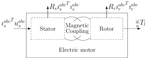
Figure 1: Power exchanges in an electric motor.

To compute the generalized forces, we notice that according to Fig. 1 the motor:

• receives the electrical power ${\imath_{s}^{abc}}^{T}u_{s}^{abc}$, where $u_{s}^{abc}$ is the vector of voltage drops across the stator windings; hence, $u_{s}^{abc}$ is a generalized force associated to the generalized coordinate $q_{s}^{abc}$

• loses the electrical power $R_{s}{\imath_{s}^{abc}}^{T}\imath_{s}^{abc}$ in its stator resistance $R_{s}$; hence, $-R_{s}\imath_{s}^{abc}$ is a generalized force associated to the generalized coordinate $q_{s}^{abc}$

• loses the electrical power $R_{r}{\imath_{r}^{abc}}^{T}{\imath_{r}^{abc}}$ in the rotor resistance $R_{r}$; hence, $-R_{r}\imath_{r}^{abc}$ is the generalized force associated to the generalized coordinate $q_{r}^{abc}$

• yields the mechanical power $\frac{\omega}{n}T_{l}$, where $T_{l}$ is the load torque; hence, $-\frac{T_{l}}{n}$ is the generalized force associated to the generalized coordinate $\theta$.

Taking into account these generalized forces, the Euler-Lagrange equations (1a) read

$$\frac{d\theta}{dt} = \omega$$ (7a)

$$\frac{d}{dt}\nabla_{\imath_{s}^{abc}}\mathcal{L}^{abc}(\imath_{s}^{abc},\imath_{r}^{abc},\theta,\omega) = u_{s}^{abc}-R_{s}\imath_{s}^{abc}$$ (8a)

$$\frac{d}{dt}\nabla_{\imath_{r}^{abc}}\mathcal{L}^{abc}(\imath_{s}^{abc},\imath_{r}^{abc},\theta,\omega) = -R_{r}\imath_{r}^{abc}$$ (9a)

$$\frac{d}{dt}\nabla_{\omega}\mathcal{L}^{abc}(\imath_{s}^{abc},\imath_{r}^{abc},\theta,\omega) = \frac{T_{e}}{n}-\frac{T_{l}}{n},$$ (10a)

where the electromagnetic torque $T_{e}$ is defined by

$$T_{e}:=n\nabla_{\theta}\mathcal{L}^{abc}(\imath_{s}^{abc},\imath_{r}^{abc},\theta,\omega);$$ (11)

as $\mathcal{L}^{abc}$ does not depend on $q_{s}^{abc}$ and $q_{r}^{abc}$, it is useless to include in (7a) the two equations

$$\frac{dq_{s}^{abc}}{dt} = \imath_{s}^{abc}$$

$$\frac{dq_{r}^{abc}}{dt} = \imath_{r}^{abc}.$$

The system (7a)-(11) is then completely defined once the scalar function $\mathcal{L}^{abc}$ is specified.

To get state equations we define the generalized momenta $p:=(\lambda_{s}^{abc},\lambda_{r}^{abc},\rho)$ associated to the generalized velocities by

$$\lambda_{s}^{abc} := \nabla_{\imath_{s}^{abc}}\mathcal{L}^{abc}(\imath_{s}^{abc},\imath_{r}^{abc},\theta,\omega)$$ (12a)

$$\lambda_{r}^{abc} := \nabla_{\imath_{r}^{abc}}\mathcal{L}^{abc}(\imath_{s}^{abc},\imath_{r}^{abc},\theta,\omega)$$ (13a)

$$\rho := n^{2}\nabla_{\omega}\mathcal{L}^{abc}(\imath_{s}^{abc},\imath_{r}^{abc},\theta,\omega);$$ (14a)

$\lambda_{s}^{abc}$ and $\lambda_{r}^{abc}$ are the flux linkages of the stator and rotor windings, and $\rho$ is the kinetic momentum. The $n^{2}$ factor in (14a) stems from the fact that the transformation $\theta=n\theta_{m}$ is not normalized, so

$$\rho=n\nabla_{\dot{\theta}_{m}}\mathcal{L}^{abc}=n\nabla_{\omega}\mathcal{L}^{abc}\cdot\nabla_{\dot{\theta}_{m}}\omega=n^{2}\nabla_{\omega}\mathcal{L}^{abc}.$$

As in (3), we define the Hamiltonian $\mathcal{H}^{abc}$ by

$$\mathcal{H}^{abc}(\lambda_{s}^{abc},\lambda_{r}^{abc},\theta,\rho):={\imath_{s}^{abc}}^{T}\!\lambda_{s}^{abc}+\omega\rho-\mathcal{L}^{abc}(\imath_{s}^{abc},\imath_{r}^{abc},\theta,\rho).$$

The state equations (4a) then read

$$\frac{d\lambda_{s}^{abc}}{dt} = u_{s}^{abc}-R_{s}\imath_{s}^{abc}$$ (15a)

$$\frac{d\lambda_{r}^{abc}}{dt} = -R_{r}\imath_{r}^{abc}$$ (16a)

$$\frac{d\theta}{dt} = \omega$$ (17a)

$$\frac{1}{n}\frac{d\rho}{dt} = T_{e}-T_{l},$$ (18a)

with

$$\imath_{s}^{abc} = \nabla_{\lambda_{s}^{abc}}\mathcal{H}^{abc}(\lambda_{s}^{abc},\lambda_{r}^{abc},\theta,\rho)$$ (19a)

$$\imath_{r}^{abc} = \nabla_{\lambda_{r}^{abc}}\mathcal{H}^{abc}(\lambda_{s}^{abc},\lambda_{r}^{abc},\theta,\rho)$$ (20a)

$$\omega = n^{2}\nabla_{\rho}\mathcal{H}^{abc}(\lambda_{s}^{abc},\lambda_{r}^{abc},\theta,\rho)$$ (21a)

$$T_{e} = -n\nabla_{\theta}\mathcal{H}^{abc}(\lambda_{s}^{abc},\lambda_{r}^{abc},\theta,\rho);$$ (22a)

as $\mathcal{H}^{abc}$ does not depend on $q_{s}^{abc}$ and $q_{r}^{abc}$, it is useless to include in (15a) the two equations

$$\frac{dq_{s}^{abc}}{dt} = \nabla_{\lambda_{s}^{abc}}\mathcal{H}^{abc}(\lambda_{s}^{abc},\lambda_{r}^{abc},\theta,\rho)$$

$$\frac{dq_{r}^{abc}}{dt} = \nabla_{\lambda_{r}^{abc}}\mathcal{H}^{abc}(\lambda_{s}^{abc},\lambda_{r}^{abc},\theta,\rho).$$

The system (15a)-(19a) is then completely defined as soon as the scalar function $\mathcal{H}^{abc}$ is given.

Notice that $\lambda_{s}^{abc}$, $\lambda_{r}^{abc}$, $\rho$ and $\theta$ are the “natural” variables to write the system in state form, and turn out to be very convenient for the analysis of models with magnetic saturation, see e.g. section VII-B. It is of course possible to rewrite (7a)-(11) in state form with the variables $\imath_{s}^{abc}$, $\imath_{r}^{abc}$, $\theta$ and $\omega$, but the resulting system is more difficult to manipulate.

section III Changing frames

The physical $abc$ frame is not very convenient for computations. It is therefore customary to rewrite the motor equations in an orthogonal frame. The constant $abc$-to-$\alpha\beta 0$ transformation is first applied. A time-varying transformation is then applied to express the stator and rotor variables in a common frame; though the general case is no more difficult to handle, we consider only the two most widely used transformations:

• the $\alpha\beta 0$-to-$dq0$ transformation, which expresses the stator and rotor variables in the frame rotating at the angular velocity $\omega_{s}=\frac{d\theta_{s}}{dt}$, where $\theta_{s}$ is the orientation of the control voltage vector; $\omega_{s}$ can be seen as a new control. This transformation is commonly used for asynchronous motors

• the $\alpha\beta 0$-to-$DQ0$ transformation, which expresses the stator variables in the rotor frame. This transformation is commonly used for synchronous motors.

III-A $abc$-to-$\alpha\beta 0$ transformation

Define the $\alpha\beta 0$ state variables

$$\lambda_{s}^{\alpha\beta 0} := \mathcal{C}\lambda_{s}^{abc}$$

$$\lambda_{r}^{\alpha\beta 0} := \mathcal{C}\lambda_{r}^{abc}$$

and the scalar function

$$\mathcal{H}^{\alpha\beta 0}(\lambda_{s}^{\alpha\beta 0},\lambda_{r}^{\alpha\beta 0},\theta,\rho):=\mathcal{H}^{abc}(\mathcal{C}^{T}\lambda_{s}^{\alpha\beta 0},\mathcal{C}^{T}\lambda_{r}^{\alpha\beta 0},\theta,\rho),$$

where $\mathcal{C}$ is the orthogonal matrix

$$\mathcal{C}:=\sqrt{\frac{2}{3}}\begin{pmatrix}1&-\frac{1}{2}&-\frac{1}{2}\\ 0&\frac{\sqrt{3}}{2}&-\frac{\sqrt{3}}{2}\\ \frac{\sqrt{2}}{2}&\frac{\sqrt{2}}{2}&\frac{\sqrt{2}}{2}\end{pmatrix}.$$

We then find

$$\frac{d\lambda_{s}^{\alpha\beta 0}}{dt} = \mathcal{C}\frac{d\lambda_{s}^{abc}}{dt}$$

$$= \mathcal{C}(u_{s}^{abc}-R_{s}\imath_{s}^{abc})$$

$$= \mathcal{C}u_{s}^{abc}-R_{s}\mathcal{C}\nabla_{\lambda_{s}^{abc}}\mathcal{H}^{abc}$$

$$= \mathcal{C}u_{s}^{abc}-R_{s}\mathcal{C}\mathcal{C}^{T}\nabla_{\lambda_{s}^{\alpha\beta 0}}\mathcal{H}^{\alpha\beta 0}$$

$$\frac{d\lambda_{r}^{\alpha\beta 0}}{dt} = -R_{r}\mathcal{C}\mathcal{C}^{T}\nabla_{\lambda_{r}^{\alpha\beta 0}}\mathcal{H}^{\alpha\beta 0}.$$

This yields

$$\frac{d\lambda_{s}^{\alpha\beta 0}}{dt} = u_{s}^{\alpha\beta 0}-R_{s}\imath_{s}^{\alpha\beta 0}$$ (23a)

$$\frac{d\lambda_{r}^{\alpha\beta 0}}{dt} = -R_{r}\imath_{r}^{\alpha\beta 0}$$ (24a)

$$\frac{d\theta}{dt} = \omega$$ (25a)

$$\frac{1}{n}\frac{d\rho}{dt} = T_{e}-T_{l},$$ (26a)

where $u_{s}^{\alpha\beta 0}:=\mathcal{C}u_{s}^{abc}$ and

$$\imath_{s}^{\alpha\beta 0} := \mathcal{C}\imath_{s}^{abc}=\nabla_{\lambda_{s}^{\alpha\beta 0}}\mathcal{H}^{\alpha\beta 0}(\lambda_{s}^{\alpha\beta 0},\lambda_{r}^{\alpha\beta 0},\theta,\rho)$$ (27a)

$$\imath_{r}^{\alpha\beta 0} := \mathcal{C}\imath_{r}^{abc}=\nabla_{\lambda_{r}^{\alpha\beta 0}}\mathcal{H}^{\alpha\beta 0}(\lambda_{s}^{\alpha\beta 0},\lambda_{r}^{\alpha\beta 0},\theta,\rho)$$ (28a)

$$\omega = n^{2}\nabla_{\rho}\mathcal{H}^{\alpha\beta 0}(\lambda_{s}^{\alpha\beta 0},\lambda_{r}^{\alpha\beta 0},\theta,\rho)$$ (29a)

$$T_{e} = -n\nabla_{\theta}\mathcal{H}^{\alpha\beta 0}(\lambda_{s}^{\alpha\beta 0},\lambda_{r}^{\alpha\beta 0},\theta,\rho).$$ (30a)

Notice that (23a)-(27a) have the same structure as (15a)-(19a), i.e., corresponds to a Hamiltonian formulation, with $(u_{s}^{\alpha\beta 0}-R_{s}\imath_{s}^{\alpha\beta 0},-R_{r}\imath_{r}^{\alpha\beta 0},-T_{l})$ as the vector of generalized forces. The $abc$-to-$\alpha\beta 0$ transformation is what is called a canonical transformation, which preserves the Hamiltonian structure.

We emphasize that (27a) and (28a) automatically enforce the reciprocity conditions which must be satisfied by any reasonable motor model [10]; indeed,

$$\frac{\partial\imath_{s}^{\alpha}}{\partial\lambda_{s}^{\beta}}=\frac{\partial^{2}\mathcal{H}^{\alpha\beta 0}}{\partial{\lambda_{s}^{\beta}}\partial{\lambda_{s}^{\alpha}}} = \frac{\partial^{2}\mathcal{H}^{\alpha\beta 0}}{\partial{\lambda_{s}^{\alpha}}\partial{\lambda_{s}^{\beta}}}=\frac{\partial\imath_{s}^{\beta}}{\partial\lambda_{s}^{\alpha}}$$

$$\frac{\partial\imath_{r}^{\alpha}}{\partial\lambda_{r}^{\beta}}=\frac{\partial^{2}\mathcal{H}^{\alpha\beta 0}}{\partial{\lambda_{r}^{\beta}}\partial{\lambda_{r}^{\alpha}}} = \frac{\partial^{2}\mathcal{H}^{\alpha\beta 0}}{\partial{\lambda_{r}^{\alpha}}\partial{\lambda_{r}^{\beta}}}=\frac{\partial\imath_{r}^{\beta}}{\partial\lambda_{r}^{\alpha}}.$$

III-B $\alpha\beta 0$-to-$dq0$ transformation

Define the $dq0$ variables

$$\lambda_{s}^{dq0} := \mathcal{R}_{3}(-\theta_{s})\lambda_{s}^{\alpha\beta 0}$$

$$\lambda_{r}^{dq0} := \mathcal{R}_{3}(\theta-\theta_{s})\lambda_{r}^{\alpha\beta 0}$$

and the scalar function

$$\mathcal{H}^{dq0}(\lambda_{s}^{dq0},\lambda_{r}^{dq0},\theta,\rho;\theta_{s})$$

$$\qquad:=\mathcal{H}^{\alpha\beta 0}\bigl{(}\mathcal{R}_{3}(\theta_{s})\lambda_{s}^{dq0},\mathcal{R}_{3}(\theta_{s}-\theta)\lambda_{r}^{dq0},\theta,\rho\bigr{)}.$$

We then find

$$\frac{d\lambda_{s}^{dq0}}{dt} = \frac{d}{dt}\bigl{(}\mathcal{R}_{3}(-\theta_{s})\lambda_{s}^{\alpha\beta 0}\bigr{)}$$

$$= \mathcal{R}_{3}(-\theta_{s})u_{s}^{\alpha\beta 0}-\mathcal{R}_{3}(-\theta_{s})R_{s}\nabla_{\lambda_{s}^{\alpha\beta 0}}\mathcal{H}^{\alpha\beta 0}$$

$$\qquad-\>\omega_{s}\mathcal{J}_{3}\mathcal{R}_{3}(-\theta_{s})\lambda_{s}^{\alpha\beta 0}$$

$$= \mathcal{R}_{3}(-\theta_{s})u_{s}^{\alpha\beta 0}-R_{s}\mathcal{R}_{3}(-\theta_{s})\mathcal{R}_{3}(\theta_{s})\nabla_{\lambda_{s}^{dq0}}\mathcal{H}^{dq0}$$

$$\qquad-\>\omega_{s}\mathcal{J}_{3}\lambda_{s}^{dq0}$$

$$\frac{d\lambda_{r}^{dq0}}{dt} = \frac{d}{dt}\left(\mathcal{R}_{3}(\theta-\theta_{s})\lambda_{r}^{\alpha\beta 0}\right)$$

$$= -\mathcal{R}_{3}(\theta-\theta_{s})R_{r}\nabla_{\lambda_{r}^{\alpha\beta 0}}\mathcal{H}^{\alpha\beta 0}$$

$$\qquad-\>(\omega_{s}-\omega)\mathcal{J}_{3}\mathcal{R}_{3}(\theta-\theta_{s})\lambda_{r}^{\alpha\beta 0}$$

$$= -R_{r}\mathcal{R}_{3}(\theta-\theta_{s})\mathcal{R}_{3}(\theta_{s}-\theta)\nabla_{\lambda_{r}^{dq0}}\mathcal{H}^{dq0}$$

$$\qquad-\>(\omega_{s}-\omega)\mathcal{J}_{3}\lambda_{r}^{dq0};$$

moreover $T_{e}=n{\lambda_{r}^{dq0}}^{T}\!\!\!\mathcal{J}_{3}\imath_{r}^{dq0}-n\nabla_{\theta}\mathcal{H}^{dq0}$, since

$$\nabla_{\theta}\mathcal{H}^{dq0} = \nabla_{\theta}\mathcal{H}^{\alpha\beta 0}+\partial_{\lambda_{r}^{\alpha\beta 0}}\mathcal{H}^{\alpha\beta 0}\nabla_{\theta}\left(\mathcal{R}_{3}(\theta_{s}-\theta)\lambda_{r}^{dq0}\right)$$

$$= \nabla_{\theta}\mathcal{H}^{\alpha\beta 0}-\partial_{\lambda_{r}^{\alpha\beta 0}}\mathcal{H}^{\alpha\beta 0}{\mathcal{R}_{3}}(\theta_{s}-\theta)\mathcal{J}_{3}\lambda_{r}^{dq0}$$

$$= \nabla_{\theta}\mathcal{H}^{\alpha\beta 0}+{\lambda_{r}^{dq0}}^{T}\!\!\!\mathcal{J}_{3}\nabla_{\lambda_{r}^{dq0}}\mathcal{H}^{dq0}.$$

Finally, the transformed system reads

$$\frac{d\lambda_{s}^{dq0}}{dt} = u_{s}^{dq0}-R_{s}\imath_{s}^{dq0}-\mathcal{J}_{3}\omega_{s}\lambda_{s}^{dq0}$$ (31a)

$$\frac{d\lambda_{r}^{dq0}}{dt} = -R_{r}\imath_{r}^{dq0}-\mathcal{J}_{3}(\omega_{s}-\omega)\lambda_{r}^{dq0}$$ (32a)

$$\frac{d\theta}{dt} = \omega$$ (33a)

$$\frac{1}{n}\frac{d\rho}{dt} = T_{e}-T_{l},$$ (34a)

where $u_{s}^{dq0}:=\mathcal{R}_{3}(-\theta_{s})\lambda_{s}^{\alpha\beta 0}$ and

$$\imath_{s}^{dq0} := \mathcal{R}_{3}(-\theta_{s})\imath_{s}^{\alpha\beta 0}$$ (35)

$$= \nabla_{\lambda_{s}^{dq0}}\mathcal{H}^{dq0}(\lambda_{s}^{dq0},\lambda_{r}^{dq0},\theta,\rho;\theta_{s})$$ (36a)

$$\imath_{r}^{dq0} := \mathcal{R}_{3}(\theta-\theta_{s})\imath_{r}^{\alpha\beta 0}$$ (37a)

$$= \nabla_{\lambda_{r}^{dq0}}\mathcal{H}^{dq0}(\lambda_{s}^{dq0},\lambda_{r}^{dq0},\theta,\rho;\theta_{s})$$

$$\omega = n^{2}\nabla_{\rho}\mathcal{H}^{dq0}(\lambda_{s}^{dq0},\lambda_{r}^{dq0},\theta,\rho;\theta_{s})$$ (38a)

$$T_{e} = -n\nabla_{\theta}\mathcal{H}^{dq0}(\lambda_{s}^{dq0},\lambda_{r}^{dq0},\theta,\rho;\theta_{s})+n{\lambda_{r}^{dq0}}^{T}\!\!\!\mathcal{J}_{3}\imath_{r}^{dq0}.$$ (39a)

The $\alpha\beta 0$-to-$dq0$ transformation is not canonical, as (31a)-(35) does not correspond to a Hamiltonian formulation, because of the new terms in the equations of the flux linkages and torque. This is not a problem for control purposes, and we can still consider $\mathcal{H}^{dq0}$ as the “pseudo-Hamiltonian” of the system. Nevertheless, the reciprocity conditions

$$\frac{\partial\imath_{s}^{d}}{\partial\lambda_{s}^{q}}=\frac{\partial\imath_{s}^{q}}{\partial\lambda_{s}^{d}},\quad \frac{\partial\imath_{r}^{d}}{\partial\lambda_{r}^{q}}=\frac{\partial\imath_{r}^{q}}{\partial\lambda_{r}^{d}}$$

are still satisfied.

III-C $\alpha\beta 0$-to-$DQ0$ transformation

Define the $DQ0$ variables by

$$\lambda_{s}^{DQ0} := \mathcal{R}_{3}(-\theta)\lambda_{s}^{\alpha\beta 0}$$

$$\lambda_{r}^{DQ0} := \lambda_{r}^{\alpha\beta 0}$$

and the scalar function

$$\mathcal{H}^{DQ0}(\lambda_{s}^{DQ0},\lambda_{r}^{DQ0},\theta,\rho):=\mathcal{H}^{\alpha\beta 0}(\mathcal{R}_{3}(\theta)\lambda_{s}^{DQ0},\lambda_{r}^{DQ0},\theta,\rho).$$

Proceeding as in the previous section, the transformed system reads

$$\frac{d\lambda_{s}^{DQ0}}{dt} = u_{s}^{DQ0}-R_{s}\imath_{s}^{DQ0}-\mathcal{J}_{3}\omega\lambda_{s}^{DQ0}$$ (40a)

$$\frac{d\lambda_{r}^{DQ0}}{dt} = -R_{r}\imath_{r}^{DQ0}$$ (41a)

$$\frac{d\theta}{dt} = \omega$$ (42a)

$$\frac{1}{n}\frac{d\rho}{dt} = T_{e}-T_{l},$$ (43a)

where $u_{s}^{DQ0}:=\mathcal{R}_{3}(-\theta)u_{s}^{\alpha\beta 0}$ and

$$\imath_{s}^{DQ0} := \mathcal{R}_{3}(-\theta)\imath_{s}^{\alpha\beta 0}=\nabla_{\!\!\lambda_{s}^{DQ0}}\mathcal{H}^{DQ0}(\lambda_{s}^{DQ0}\!\!,\lambda_{r}^{DQ0}\!\!,\theta,\rho)$$ (44a)

$$\imath_{r}^{DQ0} := \imath_{r}^{\alpha\beta 0}=\nabla_{\!\!\lambda_{r}^{DQ0}}\mathcal{H}^{DQ0}(\lambda_{s}^{DQ0},\lambda_{r}^{DQ0},\theta,\rho)$$ (45a)

$$\omega = n^{2}\nabla_{\rho}\mathcal{H}^{DQ0}(\lambda_{s}^{DQ0},\lambda_{r}^{DQ0},\theta,\rho)$$ (46a)

$$T_{e} = -n\nabla_{\theta}\mathcal{H}^{DQ0}(\lambda_{s}^{DQ0},\lambda_{r}^{DQ0},\theta,\rho)$$ (47a)

$$-\>n{\lambda_{s}^{DQ0}}^{T}\!\!\!\mathcal{J}_{3}\imath_{s}^{DQ0}.$$

The $\alpha\beta 0$-to-$DQ0$ transformation is also not canonical, but the reciprocity conditions

$$\frac{\partial\imath_{s}^{D}}{\partial{\lambda_{s}^{Q}}}=\frac{\partial\imath_{s}^{Q}}{\partial{\lambda_{s}^{D}}},\quad \frac{\partial\imath_{r}^{D}}{\partial\lambda_{r}^{Q}}=\frac{\partial\imath_{r}^{Q}}{\partial\lambda_{r}^{D}}$$

are once again satisfied.

III-D Summary: equations in a general $xyz$ frame

We can summarize the models obtained in the frames $abc$, $\alpha\beta 0$, $dq0$ and $DQ0$ by writing them in a general $xyz$ frame. The state equations (15a), (23a), (31a) and (40a) then read

$$\frac{d\lambda_{s}^{xyz}}{dt} = u_{s}^{xyz}-R_{s}\imath_{s}^{xyz}-\mathcal{J}_{3}\Omega^{xyz}_{s}\lambda_{s}^{xyz}$$ (48a)

$$\frac{d\lambda_{r}^{xyz}}{dt} = -R_{r}\imath_{r}^{xyz}-\mathcal{J}_{3}\Omega^{xyz}_{r}\lambda_{r}^{xyz}$$ (49a)

$$\frac{d\theta}{dt} = \omega$$ (50a)

$$\frac{1}{n}\frac{d\rho}{dt} = T_{e}-T_{l},$$ (51a)

while the constitutive relations (19a), (27a), (35) and (44a) read

$$\imath_{s}^{xyz} = \nabla_{\lambda_{s}^{xyz}}\mathcal{H}^{xyz}(\lambda_{s}^{xyz},\lambda_{r}^{xyz},\theta,\rho)$$ (52a)

$$\imath_{r}^{xyz} = \nabla_{\lambda_{r}^{xyz}}\mathcal{H}^{xyz}(\lambda_{s}^{xyz},\lambda_{r}^{xyz},\theta,\rho)$$ (53a)

$$\omega = n^{2}\nabla_{\rho}\mathcal{H}^{xyz}(\lambda_{s}^{xyz},\lambda_{r}^{xyz},\theta,\rho)$$ (54a)

$$T_{e} = -n\nabla_{\theta}\mathcal{H}^{xyz}(\lambda_{s}^{xyz},\lambda_{r}^{xyz},\theta,\rho)+T_{e}^{xyz}.$$ (55a)

In (48a)-(52a), the frame-specific terms are characterized by

$$(\Omega_{s}^{abc},\Omega_{r}^{abc},T_{e}^{abc}) = (0,0,0)$$ (56a)

$$(\Omega_{s}^{\alpha\beta 0},\Omega_{r}^{\alpha\beta 0},T_{e}^{\alpha\beta 0}) = (0,0,0)$$ (57a)

$$(\Omega_{s}^{dq0},\Omega_{r}^{dq0},T_{e}^{dq0}) = (\omega_{s},\omega_{s}-\omega,n\lambda_{r}^{dq0}\mathcal{J}_{3}\imath_{r}^{dq0})$$ (58a)

$$(\Omega_{s}^{DQ0},\Omega_{r}^{DQ0},T_{e}^{DQ0}) = (\omega,0,-n\lambda_{s}^{DQ0}\mathcal{J}_{3}\imath_{s}^{DQ0}).$$ (59a)

These frame-specific terms are not zero in the $dq0$ and $DQ0$ frames, because the transformations to these frames are not canonical, hence (48a)-(52a) is in these cases only a “pseudo-Hamiltonian” formulation.

section IV Using geometric symmetries of AC motors

The geometric symmetries enjoyed by any well-built motor constrain the form of its Hamiltonian, which facilitates its determination. The idea is simple: when a symmetry leaves the motor globally unchanged (meaning the new geometric configuration is indistinguishable from the original one), then the Hamiltonian is also unchanged.

IV-A Stator symmetry: circular permutation of stator phases

If the three stator phases, which are identical, are circularly permuted, and the rotor is rotated by $\frac{2\pi}{3}$, the motor is globally unchanged: indeed, rotating it by $-\frac{2\pi}{3}$ gives back the initial configuration. The Hamiltonian must therefore satisfy

$$\mathcal{H}^{abc}(\lambda_{s}^{abc},\lambda_{r}^{abc},\theta,\rho)=\mathcal{H}^{abc}\bigl{(}\mathcal{P}^{abc}\lambda_{s}^{abc},\lambda_{r}^{abc},\theta+\tfrac{2\pi}{3},\rho\bigr{)},$$

where the phase permutation matrix $\mathcal{P}^{abc}$ is defined as

$$\mathcal{P}^{abc}:=\begin{pmatrix}0&0&1\\ 1&0&0\\ 0&1&0\end{pmatrix}.$$

In the $\alpha\beta 0$ frame, this invariance property reads

$$\mathcal{H}^{\alpha\beta 0}\bigl{(}\lambda_{s}^{\alpha\beta 0},\lambda_{r}^{\alpha\beta 0},\theta,\rho\bigr{)}$$

$$\qquad=\mathcal{H}^{abc}\bigl{(}\mathcal{C}^{T}\lambda_{s}^{\alpha\beta 0},\mathcal{C}^{T}\lambda_{r}^{\alpha\beta 0},\theta,\rho\bigr{)}$$

$$\qquad=\mathcal{H}^{abc}\bigl{(}\mathcal{P}^{abc}\mathcal{C}^{T}\lambda_{s}^{\alpha\beta 0},\mathcal{C}^{T}\lambda_{r}^{\alpha\beta 0},\theta+\tfrac{2\pi}{3},\rho\bigr{)}$$

$$\qquad=\mathcal{H}^{\alpha\beta 0}\bigl{(}\mathcal{C}\mathcal{P}^{abc}\mathcal{C}^{T}\lambda_{s}^{\alpha\beta 0},\mathcal{C}\mathcal{C}^{T}\lambda_{r}^{\alpha\beta 0},\theta+\tfrac{2\pi}{3},\rho\bigr{)}$$

$$\qquad=\mathcal{H}^{\alpha\beta 0}\bigl{(}\mathcal{R}_{3}(\tfrac{2\pi}{3})\lambda_{s}^{\alpha\beta 0},\lambda_{r}^{\alpha\beta 0},\theta+\tfrac{2\pi}{3},\rho\bigr{)}.$$

In the $DQ0$ frame, this property is particularly simple,

$$\mathcal{H}^{DQ0}\bigl{(}\lambda_{s}^{DQ0},\lambda_{r}^{DQ0},\theta,\rho\bigr{)}$$ (60)

$$\qquad=\mathcal{H}^{\alpha\beta 0}\bigl{(}\mathcal{R}_{3}(\theta)\lambda_{s}^{DQ0},\lambda_{r}^{DQ0},\theta,\rho\bigr{)}$$

$$\qquad=\mathcal{H}^{\alpha\beta 0}\bigl{(}\mathcal{R}_{3}(\tfrac{2\pi}{3})\mathcal{R}_{3}(\theta)\lambda_{s}^{DQ0},\lambda_{r}^{DQ0},\theta+\tfrac{2\pi}{3},\rho\bigr{)}$$

$$\qquad=\mathcal{H}^{DQ0}\bigl{(}\mathcal{R}_{3}(-\theta-\tfrac{2\pi}{3})\mathcal{R}_{3}(\tfrac{2\pi}{3})\mathcal{R}_{3}(\theta)\lambda_{s}^{DQ0},$$

$$\qquad\qquad\lambda_{r}^{DQ0},\theta+\tfrac{2\pi}{3},\rho\bigr{)}$$

$$\qquad=\mathcal{H}^{DQ0}\bigl{(}\lambda_{s}^{DQ0},\lambda_{r}^{DQ0},\theta+\tfrac{2\pi}{3},\rho\bigr{)};$$ (61)

in other words, the Hamiltonian in the $DQ0$ frame is $\frac{2\pi}{3}$-periodic with respect to $\theta$. Finally, in the $dq0$ frame,

$$\mathcal{H}^{dq0}\bigl{(}\lambda_{s}^{dq0},\lambda_{r}^{dq0},\theta,\rho\bigr{)}$$ (62)

$$\qquad=\mathcal{H}^{\alpha\beta 0}\bigl{(}\mathcal{R}_{3}(\theta_{s})\lambda_{s}^{dq0},\mathcal{R}_{3}(\theta_{s}-\theta)\lambda_{r}^{dq0},\theta,\rho\bigr{)}$$

$$\qquad=\mathcal{H}^{\alpha\beta 0}\bigl{(}\mathcal{R}_{3}(\tfrac{2\pi}{3})\mathcal{R}_{3}(\theta_{s})\lambda_{s}^{dq0},$$

$$\qquad\qquad\mathcal{R}_{3}(\theta_{s}-\theta)\lambda_{r}^{dq0},\theta+\tfrac{2\pi}{3},\rho\bigr{)}$$

$$\qquad=\mathcal{H}^{dq0}\bigl{(}\mathcal{R}_{3}(-\theta_{s})\mathcal{R}_{3}(\tfrac{2\pi}{3})\mathcal{R}_{3}(\theta_{s})\lambda_{s}^{dq0},$$

$$\qquad\qquad\mathcal{R}_{3}(\theta+\tfrac{2\pi}{3}-\theta_{s})\mathcal{R}_{3}(\theta_{s}-\theta)\lambda_{r}^{dq0},\theta+\tfrac{2\pi}{3},\rho\bigr{)}$$

$$\qquad=\mathcal{H}^{dq0}\bigl{(}\mathcal{R}_{3}(\tfrac{2\pi}{3})\lambda_{s}^{dq0},\mathcal{R}_{3}(\tfrac{2\pi}{3})\lambda_{r}^{dq0},\theta+\tfrac{2\pi}{3},\rho\bigr{)}.$$ (63)

IV-B Stator symmetry: reversal of stator flux linkages

As the opposite poles of the stator are identical, if the stator flux linkages are reversed and the rotor is rotated by $\pi$, the motor is globally unchanged: indeed, rotating it by $-\pi$ gives back the initial configuration. The Hamiltonian must therefore satisfy

$$\mathcal{H}^{abc}(\lambda_{s}^{abc},\lambda_{r}^{abc},\theta,\rho)=\mathcal{H}^{abc}(-\lambda_{s}^{abc},\lambda_{r}^{abc},\theta+\pi,\rho).$$

Proceeding as in the previous section, this yields

$$\mathcal{H}^{\alpha\beta 0}(\lambda_{s}^{\alpha\beta 0},\lambda_{r}^{\alpha\beta 0},\theta,\rho)$$ (64)

$$\qquad=\mathcal{H}^{\alpha\beta 0}(-\lambda_{s}^{\alpha\beta 0},\lambda_{r}^{\alpha\beta 0},\theta+\pi,\rho)$$

$$\mathcal{H}^{DQ0}({\lambda_{s}^{D}},{\lambda_{s}^{Q}},\lambda_{s}^{0},\lambda_{r}^{D},\lambda_{r}^{Q},\lambda_{r}^{0},\theta,\rho)$$

$$\qquad=\mathcal{H}^{DQ0}({\lambda_{s}^{D}},{\lambda_{s}^{Q}},-\lambda_{s}^{0},\lambda_{r}^{D},\lambda_{r}^{Q},\lambda_{r}^{0},\theta+\pi,\rho)$$ (65)

$$\mathcal{H}^{dq0}(\lambda_{s}^{d},\lambda_{s}^{q},\lambda_{s}^{0},\lambda_{r}^{d},\lambda_{r}^{q},\lambda_{r}^{0},\theta,\rho)$$

$$\qquad=\mathcal{H}^{dq0}(-\lambda_{s}^{d},-\lambda_{s}^{q},-\lambda_{s}^{0},-\lambda_{r}^{d},-\lambda_{r}^{q},\lambda_{r}^{0},\theta+\pi,\rho).$$ (66)

IV-C Rotor symmetry: reversal of rotor flux linkages

As the opposite poles of the rotor are identical, if the rotor flux linkages are reversed and the rotor is rotated by $\pi$, the motor is globally unchanged: indeed, rotating it by $-\pi$ gives back the initial configuration. The Hamiltonian must therefore satisfy

$$\mathcal{H}^{abc}(\lambda_{s}^{abc},\lambda_{r}^{abc},\theta,\rho)=\mathcal{H}^{abc}(\lambda_{s}^{abc},-\lambda_{r}^{abc},\theta+\pi,\rho).$$

Proceeding as in the previous section, this yields

$$\mathcal{H}^{\alpha\beta 0}(\lambda_{s}^{\alpha\beta 0},\lambda_{r}^{\alpha\beta 0},\theta,\rho)$$ (67)

$$\qquad=\mathcal{H}^{\alpha\beta 0}(\lambda_{s}^{\alpha\beta 0},-\lambda_{r}^{\alpha\beta 0},\theta+\pi,\rho)$$

$$\mathcal{H}^{DQ0}({\lambda_{s}^{D}},{\lambda_{s}^{Q}},\lambda_{s}^{0},\lambda_{r}^{D},\lambda_{r}^{Q},\lambda_{r}^{0},\theta,\rho)$$

$$\qquad=\mathcal{H}^{DQ0}(-{\lambda_{s}^{D}}\!,-{\lambda_{s}^{Q}}\!,\lambda_{s}^{0},-\lambda_{r}^{D}\!,-\lambda_{r}^{Q}\!,-\lambda_{r}^{0},\theta+\pi,\rho)$$ (68)

$$\mathcal{H}^{dq0}(\lambda_{s}^{d},\lambda_{s}^{q},\lambda_{s}^{0},\lambda_{r}^{q},\lambda_{r}^{q},\lambda_{r}^{0},\theta,\rho)$$

$$\qquad=\mathcal{H}^{dq0}(\lambda_{s}^{d},\lambda_{s}^{q},\lambda_{s}^{0},\lambda_{r}^{d},\lambda_{r}^{q},-\lambda_{r}^{0},\theta+\pi,\rho).$$ (69)

IV-D Rotor symmetry: circular permutation of rotor phases/bars

In an induction motor, the rotor is invariant by a rotation of angle $\eta$; for a wound-rotor motor $\eta=\frac{2\pi}{3}$, since the three phases are identical; for a squirrel-cage motor $\eta=\frac{2\pi}{n_{r}}$ (with $n_{r}$ the number of bars per pole pair), since the bars are identical. Though this is a symmetry in the $abc$ frame, it is easier to express it in the $\alpha\beta 0$ frame: if the rotor flux linkage is rotated by $-\eta$ around the $0$-axis and the rotor is rotated by $\eta$, the motor is globally unchanged. The Hamiltonian must therefore satisfy

$$\mathcal{H}^{\alpha\beta 0}(\lambda_{s}^{\alpha\beta 0}\!,\lambda_{r}^{\alpha\beta 0}\!,\theta,\rho)=\mathcal{H}^{\alpha\beta 0}\bigl{(}\lambda_{s}^{\alpha\beta 0}\!,\mathcal{R}_{3}(-\eta)\lambda_{r}^{\alpha\beta 0}\!,\theta+\eta,\rho\bigr{)}.$$

In the $dq0$ frame,

$$\mathcal{H}^{dq0}\bigl{(}\lambda_{s}^{dq0},\lambda_{r}^{dq0},\theta,\rho\bigr{)}$$ (70)

$$\qquad=\mathcal{H}^{\alpha\beta 0}\bigl{(}\mathcal{R}_{3}(\theta_{s})\lambda_{s}^{dq0},\mathcal{R}_{3}(\theta_{s}-\theta)\lambda_{r}^{dq0},\theta+\eta,\rho\bigr{)}$$

$$\qquad=\mathcal{H}^{\alpha\beta 0}\bigl{(}\mathcal{R}_{3}(\theta_{s})\lambda_{s}^{dq0},\mathcal{R}_{3}(-\eta)\mathcal{R}_{3}(\theta_{s}-\theta)\lambda_{r}^{dq0},\theta+\eta,\rho\bigr{)}$$

$$\qquad=\mathcal{H}^{dq0}\bigl{(}\mathcal{R}_{3}(-\theta_{s})\mathcal{R}_{3}(\theta_{s})\lambda_{s}^{dq0},$$

$$\qquad\qquad\mathcal{R}_{3}(\theta+\eta-\theta_{s})\mathcal{R}_{3}(-\eta)\mathcal{R}_{3}(\theta_{s}-\theta)\lambda_{r}^{dq0},\theta+\eta,\rho\bigr{)}$$

$$\qquad=\mathcal{H}^{dq0}(\lambda_{s}^{dq0},\lambda_{r}^{dq0},\theta+\eta,\rho).$$ (71)

IV-E Stator and rotor symmetry: exchange of phases

When the rotor is symmetric with respect to a plane (without loss of generality the $a$-axis belongs to this plane), if the $b$ and $c$ phases are swapped in both the stator and the rotor, and the direction of the rotation is reversed, the motor is globally unchanged: indeed, a reflection gives back the initial configuration. The Hamiltonian must therefore satisfy

$$\mathcal{H}^{abc}(\lambda_{s}^{abc},\lambda_{r}^{abc},\theta,\rho)=\mathcal{H}^{abc}(\mathcal{O}^{abc}\lambda_{s}^{abc},\mathcal{O}^{abc}\lambda_{r}^{abc},-\theta,-\rho),$$

where

$$\mathcal{O}^{abc}:=\begin{pmatrix}1&0&0\\ 0&0&1\\ 0&1&0\end{pmatrix}.$$

Expressed in the $\alpha\beta 0$ frame, this reads

$$\mathcal{H}^{\alpha\beta 0}(\lambda_{s}^{\alpha\beta 0},\lambda_{r}^{\alpha\beta 0},\theta,\rho)$$

$$\qquad=\mathcal{H}^{\alpha\beta 0}(\mathcal{O}^{\alpha\beta 0}\lambda_{s}^{\alpha\beta 0},\mathcal{O}^{\alpha\beta 0}\lambda_{r}^{\alpha\beta 0},-\theta,-\rho),$$

where

$$\mathcal{O}^{\alpha\beta 0}:=\mathcal{C}\mathcal{O}^{abc}\mathcal{C}^{-1}=\begin{pmatrix}1&0&0\\ 0&-1&0\\ 0&0&1\end{pmatrix}.$$

In the $DQ0$ and $dq0$ frames,

$$\mathcal{H}^{DQ0}\bigl{(}\lambda_{s}^{DQ0},\lambda_{r}^{DQ0},\theta,\rho\bigr{)}$$

$$\qquad=\mathcal{H}^{\alpha\beta 0}\bigl{(}\mathcal{R}_{3}(\theta)\lambda_{s}^{DQ0},\lambda_{r}^{DQ0},\theta,\rho\bigr{)}$$

$$\qquad=\mathcal{H}^{\alpha\beta 0}\bigl{(}\mathcal{O}^{\alpha\beta 0}\mathcal{R}_{3}(\theta)\lambda_{s}^{DQ0},\mathcal{O}^{\alpha\beta 0}\lambda_{r}^{DQ0},-\theta,-\rho\bigr{)}$$

$$\qquad=\mathcal{H}^{DQ0}\bigl{(}\mathcal{R}_{3}(\theta)\mathcal{O}^{\alpha\beta 0}\mathcal{R}_{3}(\theta)\lambda_{s}^{DQ0},$$

$$\qquad\qquad\mathcal{O}^{\alpha\beta 0}\lambda_{r}^{DQ0},-\theta,-\rho\bigr{)}$$

$$\mathcal{H}^{dq0}\bigl{(}\lambda_{s}^{dq0},\lambda_{r}^{dq0},\theta,\rho\bigr{)}$$

$$\qquad=\mathcal{H}^{dq0}\bigl{(}\mathcal{R}_{3}(\theta_{s})\mathcal{O}^{\alpha\beta 0}\mathcal{R}_{3}(\theta_{s})\lambda_{s}^{dq0},$$

$$\qquad\qquad\mathcal{R}_{3}(\theta_{s}-\theta)\mathcal{O}^{\alpha\beta 0}\mathcal{R}_{3}(\theta_{s}-\theta)\lambda_{r}^{dq0},-\theta,-\rho\bigr{)}.$$

Rewritten component-wise, this yields the parity conditions

$$\mathcal{H}^{DQ0}({\lambda_{s}^{D}},{\lambda_{s}^{Q}},\lambda_{s}^{0},\lambda_{r}^{D},\lambda_{r}^{Q},\lambda_{r}^{0},\theta,\rho)$$ (72)

$$\qquad=\mathcal{H}^{DQ0}({\lambda_{s}^{D}},-{\lambda_{s}^{Q}},\lambda_{s}^{0},\lambda_{r}^{D},-\lambda_{r}^{Q},\lambda_{r}^{0},-\theta,-\rho)$$ (73)

$$\mathcal{H}^{dq0}(\lambda_{s}^{d},\lambda_{s}^{q},\lambda_{s}^{0},\lambda_{r}^{d},\lambda_{r}^{q},\lambda_{r}^{0},\theta,\rho)$$

$$\qquad=\mathcal{H}^{dq0}(\lambda_{s}^{d},-\lambda_{s}^{q},\lambda_{s}^{0},\lambda_{r}^{d},-\lambda_{r}^{q},\lambda_{r}^{0},-\theta,-\rho).$$ (74)

If the rotor is moreover symmetric with respect to the orthogonal plane, the same reasoning yields

$$\mathcal{H}^{DQ0}({\lambda_{s}^{D}},{\lambda_{s}^{Q}},\lambda_{s}^{0},\lambda_{r}^{D},\lambda_{r}^{Q},\lambda_{r}^{0},\theta,\rho)$$ (75)

$$\qquad=\mathcal{H}^{DQ0}(-{\lambda_{s}^{D}},{\lambda_{s}^{Q}},\lambda_{s}^{0},-\lambda_{r}^{D},\lambda_{r}^{Q},\lambda_{r}^{0},-\theta,-\rho)$$ (76)

$$\mathcal{H}^{dq0}(\lambda_{s}^{d},\lambda_{s}^{q},\lambda_{s}^{0},\lambda_{r}^{d},\lambda_{r}^{q},\lambda_{r}^{0},\theta,\rho)$$

$$\qquad=\mathcal{H}^{dq0}(-\lambda_{s}^{d},\lambda_{s}^{q},\lambda_{s}^{0},-\lambda_{r}^{d},\lambda_{r}^{q},\lambda_{r}^{0},-\theta,-\rho).$$ (77)

section V Using connection constraints

Up to now, we have been considering AC motors with unconnected windings. In this section, we take these connections into account, which imposes constraints on the currents involved in the equations derived in section II-B. We first study how to handle constraints in the general framework of analytical mechanics and then apply this to AC motors.

V-A Analytical mechanics with constraints (see e.g. [14])

Constraints in analytical mechanics are of two kinds: holonomic constraints $g(q)=0$, where $g(q)\in\mathbb{R}^{m}$; nonholonomic constraints $K(q)\dot{q}-k(q)=0$, where $K(q)$ is a full-rank $m\times n$ matrix and $k(q)\in\mathbb{R}^{m}$. Notice that in view of (1a) the holonomic constraint $g(q)=0$ naturally gives rise to the nonholonomic constraint $g^{\prime}(q)\dot{q}=0$; this nonholonomic constraint is equivalent to the original holonomic constraint, up to a constant which is determined by the initial value $q(0)$. The holonomic constraint $g(q)=0$ can thus be handled in two (equivalent) ways: on the one hand, assuming it is explicitly solvable as $q_{2}=h(q_{1})$, we can define the reduced Lagrangian

$$\mathcal{L}_{r}(q_{1},\dot{q}_{1}):=\mathcal{L}\bigl{(}q_{1},h(q_{1}),\dot{q}_{1},h^{\prime}(q_{1})\dot{q}_{1}\bigr{)},$$

and proceed exactly as in section II-A with $\mathcal{L}_{r}$ instead of $\mathcal{L}$; on the other hand, rather than explicitly solving the constraint, which may be cumbersome in practice, we can consider only the associated nonholonomic constraint $g^{\prime}(q)\dot{q}=0$, and handle it as any other nonholonomic constraint.

The nonholonomic constraint $K(q)\dot{q}-k(q)=0$ is handled by introducing the so-called Lagrange multiplier $\mu\in\mathbb{R}^{m}$ and using the constrained version of the Euler-Lagrange equations

$$\frac{dq}{dt} = \dot{q}$$ (78a)

$$\frac{d}{dt}\nabla_{\dot{q}}\mathcal{L} = \nabla_{q}\mathcal{L}(q,\dot{q})+\mathcal{F}+K^{T}(q)\mu$$ (79a)

$$0 = K(q)\dot{q}-k(q).$$ (80a)

To obtain the Hamiltonian formulation, we then proceed as in section II-A, but use (78a)-(79a) instead of (1a). This yields

$$\frac{dp}{dt} = -\nabla_{q}\mathcal{H}(p,q)+\mathcal{F}+K^{T}(q)\mu$$ (81a)

$$\frac{dq}{dt} = \nabla_{p}\mathcal{H}(p,q)$$ (82a)

$$0 = K(q)\nabla_{p}\mathcal{H}(p,q)-k(q),$$ (83a)

where we have replaced $\dot{q}$ in (80a) by its expression (82a). This is a differential-algebraic system with $2n$ differential equations and $m$ algebraic constraints for the $2n+m$ unknowns $p$, $q$ and $\mu$. Of course, the initial condition $(p_{0},q_{0})$ must respect the constraint (83a).

Such a differential-algebraic may be difficult to handle, e.g. for simulation purposes. If needed, (81a) may be rewritten as a purely differential system: first differentiate the constraint (83a) and use (81a)-(82a), which yields

$$0 = K\Bigl{(}\partial_{p}\nabla_{p}\mathcal{H}\frac{dp}{dt}+\partial_{q}\nabla_{p}\mathcal{H}\frac{dq}{dt}\Bigr{)}+\Bigl{(}K^{\prime}\frac{dq}{dt}\Bigr{)}\nabla_{p}\mathcal{H}-k^{\prime}\frac{dq}{dt}$$

$$= K\partial_{p}\nabla_{p}\mathcal{H}K^{T}\mu+K\partial_{p}\nabla_{p}\mathcal{H}(\mathcal{F}-\nabla_{q}\mathcal{H})$$

$$\qquad+\bigr{(}K\partial_{q}\nabla_{p}\mathcal{H}+K^{\prime}\nabla_{p}\mathcal{H}-k^{\prime}\bigl{)}\nabla_{p}\mathcal{H};$$

since $K$ is full rank and $\partial_{p}\nabla_{p}\mathcal{H}$ is invertible by assumption, $K\partial_{p}\nabla_{p}\mathcal{H}K^{T}$ is invertible and the previous equation can be solved for the Lagrange multiplier as

$$\mu=\mathcal{M}(p,q,\mathcal{F}).$$ (84)

The purely differential version of (81a) is then

$$\frac{dp}{dt} = -\nabla_{q}\mathcal{H}(p,q)+\mathcal{F}+K^{T}(q)\mathcal{M}(p,q,\mathcal{F})$$ (85a)

$$\frac{dq}{dt} = \nabla_{p}\mathcal{H}(p,q),$$ (86a)

which can be readily simulated starting from any initial condition $(p_{0},q_{0})$ such that $K(q_{0})\nabla_{p}\mathcal{H}(p_{0},q_{0})-k(q_{0})=0$.

V-B Short-circuited rotor windings

The rotor windings of AC motors are usually short-circuited, see Fig. 2a, which imposes the constraint $\imath_{r}^{a}+\imath_{r}^{b}+\imath_{r}^{c}=0$. In any frame $xy0$, this constraint reads

$$0=\imath_{r}^{0}:=\nabla_{\lambda_{r}^{0}}\mathcal{H}^{xy0}(\lambda_{s}^{xy0},\lambda_{r}^{xy},\lambda_{r}^{0},\theta,\rho);$$ (87)

if the (pseudo)-Hamiltonian is not degenerate, then $\partial_{\lambda_{r}^{0}}\nabla_{\lambda_{r}^{0}}\mathcal{H}^{xy0}\neq 0$, and $\lambda_{r}^{0}=\Lambda_{r}^{0}(\lambda_{s}^{xy0},\lambda_{r}^{xy},\theta,\rho)$ by the implicit function theorem. Define now the function

$$\mathcal{H}_{c}^{xy0}(\lambda_{s}^{xy0},\lambda_{r}^{xy},\theta,\rho)$$

$$\qquad:=\mathcal{H}^{xy0}\bigl{(}\lambda_{s}^{xy0},\lambda_{r}^{xy},\Lambda_{r}^{0}(\lambda_{s}^{xy0},\lambda_{r}^{xy},\theta,\rho),\theta,\rho\bigr{)}.$$

Its gradients with respect to $\chi\in\{\lambda_{s}^{xy0},\lambda_{r}^{xy},\theta,\rho\}$ are

$$\nabla_{\chi}\mathcal{H}_{c}^{xy0}(\lambda_{s}^{xy0},\lambda_{r}^{xy},\theta,\rho)$$

$$\quad=\nabla_{\chi}\mathcal{H}^{xy0}(\ldots)+\nabla_{\chi}\Lambda_{r}^{0}(\ldots)\nabla_{\lambda_{r}^{0}}\mathcal{H}^{xy0}(\ldots)$$

$$\quad=\nabla_{\chi}\mathcal{H}^{xy0}\bigl{(}\lambda_{s}^{xy0},\lambda_{r}^{xy},\Lambda_{r}^{0}(\lambda_{s}^{xy0},\lambda_{r}^{xy},\theta,\rho),\theta,\rho\bigr{)},$$

where $\nabla_{\lambda_{r}^{0}}\mathcal{H}^{xy0}(\ldots)=0$ by (87). The (pseudo)-Hamiltonian equations (48a)-(52a) with constraint (87) then split into two decoupled subsystems:

• the unconstrained $xy$-subsystem, with state equations

  $$\frac{d\lambda_{s}^{xy0}}{dt} = u_{s}^{xy0}-R_{s}\imath_{s}^{xy0}-\mathcal{J}_{3}\Omega^{xy0}_{s}\lambda_{s}^{xy0}$$ (88a)

  $$\frac{d\lambda_{r}^{xy}}{dt} = -R_{r}\imath_{r}^{xy}-\mathcal{J}_{2}\Omega^{xy0}_{r}\lambda_{r}^{xy}$$ (89a)

  $$\frac{d\theta}{dt} = \omega$$ (90a)

  $$\frac{1}{n}\frac{d\rho}{dt} = T_{e}-T_{l},$$ (91a)

  and constitutive relations

  $$\imath_{s}^{xy0} = \nabla_{\lambda_{s}^{xy0}}\mathcal{H}_{c}^{xy0}(\lambda_{s}^{xy0},\lambda_{r}^{xy},\theta,\rho)$$ (92a)

  $$\imath_{r}^{xy} = \nabla_{\lambda_{r}^{xy}}\mathcal{H}_{c}^{xy0}(\lambda_{s}^{xy0},\lambda_{r}^{xy},\theta,\rho)$$ (93a)

  $$\omega = n^{2}\nabla_{\rho}\mathcal{H}_{c}^{xy0}(\lambda_{s}^{xy0},\lambda_{r}^{xy},\theta,\rho)$$ (94a)

  $$T_{e} = -n\nabla_{\theta}\mathcal{H}_{c}^{xy0}(\lambda_{s}^{xy0},\lambda_{r}^{xy},\theta,\rho)+T_{e}^{xy0};$$ (95a)

  notice $T_{e}^{dq0}=n\lambda_{r}^{dq0}\mathcal{J}_{3}\imath_{r}^{dq0}=n\lambda_{r}^{dq}\mathcal{J}_{2}\imath_{r}^{dq}$ by (48a)

• the constrained $0$-subsystem

  $$\frac{d\lambda_{r}^{0}}{dt} = \mu$$ (96a)

  $$0 = \nabla_{\lambda_{r}^{0}}\mathcal{H}^{xy0}(\lambda_{s}^{xy0},\lambda_{r}^{xy},\lambda_{r}^{0},\theta,\rho).$$ (97a)

  For simulation purposes, $\mu$ can be computed as a function of the state variables using (84). Notice $\mu/\sqrt{3}$ can be seen as the voltage drop across the short-circuited windings $a$, $b$ and $c$, see Fig. 2a.

(a) Short-circuited rotor windings.

(b) Fictitious windings.

Figure 2: Main rotor connection schemes.

V-C No rotor windings

PMSMs and SynRMs do not have rotor windings, which can be translated into the 3-dimensional constraint

$$0=\imath_{r}^{xyz}(\lambda_{s}^{xyz},\lambda_{r}^{xyz},\theta,\rho):=\nabla_{\lambda_{r}^{xyz}}\mathcal{H}^{xyz}(\lambda_{s}^{xyz},\lambda_{r}^{xyz},\theta,\rho)$$

in any frame $xyz$; this simply means there are no currents in the (fictitious) rotor windings. Proceeding then exactly as in section V-B, we can invert the constraint and define the function

$$\mathcal{H}_{0}^{xyz}(\lambda_{s}^{xyz},\theta,\rho):=\mathcal{H}^{xyz}\bigl{(}\lambda_{s}^{xyz},\Lambda_{r}^{xyz}(\lambda_{s}^{xyz},\theta,\rho),\theta,\rho\bigr{)},$$

yielding the two decoupled subsystems:

• the unconstrained stator subsystem, with state equations

  $$\frac{d\lambda_{s}^{xyz}}{dt} = u_{s}^{xyz}-R_{s}\imath_{s}^{xyz}-\mathcal{J}_{3}\Omega^{xyz}_{s}\lambda_{s}^{xyz}$$ (98a)

  $$\frac{d\theta}{dt} = \omega$$ (99a)

  $$\frac{1}{n}\frac{d\rho}{dt} = T_{e}-T_{l},$$ (100a)

  and constitutive relations

  $$\imath_{s}^{xyz} = \nabla_{\lambda_{s}^{xyz}}\mathcal{H}_{0}^{xyz}(\lambda_{s}^{xyz},\theta,\rho)$$ (101a)

  $$\omega = n^{2}\nabla_{\rho}\mathcal{H}_{0}^{xyz}(\lambda_{s}^{xyz},\theta,\rho)$$ (102a)

  $$T_{e} = -n\nabla_{\theta}\mathcal{H}_{0}^{xyz}(\lambda_{s}^{xyz},\theta,\rho)+T_{e}^{xyz};$$ (103a)

  notice $T_{e}^{dq0}=n\lambda_{r}^{dq0}\mathcal{J}_{3}\imath_{r}^{dq0}=0$, see (48a)

• the (3-dimensional) constrained rotor subsystem

  $$\frac{d\lambda_{r}^{xyz}}{dt} = \mu-\mathcal{J}_{3}\Omega^{xyz}_{r}\lambda_{r}^{xyz}$$ (104a)

  $$0 = \nabla_{\lambda_{r}^{xyz}}\mathcal{H}^{xyz}(\lambda_{s}^{xyz},\lambda_{r}^{xyz},\theta,\rho).$$ (105a)

  For simulation purposes, $\mu$ can be computed as a function of the state variables using (84). Notice $\mu$ can be seen as the vector $(\mu^{a},\mu^{b},\mu^{c})$ of voltage drops across the (fictitious) rotor windings $a$, $b$ and $c$, see Fig. 2b.

V-D Star connection scheme

The stator windings of AC motors are usually star-connected, see Fig. 3b, which imposes the constraint $\imath_{s}^{a}+\imath_{s}^{b}+\imath_{s}^{c}=0$. In this connection scheme, the potentials $v_{s}^{a}$, $v_{s}^{b}$ and $v_{s}^{c}$ are impressed, and not the voltages drops across the windings. The constrained version of (15a) reads

$$\frac{d\lambda_{s}^{abc}}{dt}=u_{s}^{abc}-R_{s}\imath_{s}^{abc}+\frac{1}{\sqrt{3}}\begin{pmatrix}1\\ 1\\ 1\end{pmatrix}\mu.$$

Notice the voltage drops across the windings are by definition

$$v_{s}^{a}-v_{N} := \frac{d\lambda_{s}^{a}}{dt}+R_{s}\imath_{s}^{a}=u_{s}^{a}+\mu/\sqrt{3}$$

$$v_{s}^{b}-v_{N} := \frac{d\lambda_{s}^{b}}{dt}+R_{s}\imath_{s}^{b}=u_{s}^{b}+\mu/\sqrt{3}$$

$$v_{s}^{c}-v_{N} := \frac{d\lambda_{s}^{c}}{dt}+R_{s}\imath_{s}^{c}=u_{s}^{c}+\mu/\sqrt{3}.$$

In any frame $xy0$, this gives

$$v_{s}^{xy} = u_{s}^{xy}$$ (106a)

$$v_{s}^{0}-\sqrt{3}v_{N} = u_{s}^{0}+\mu,$$ (107a)

and the constraint $\imath_{s}^{a}+\imath_{s}^{b}+\imath_{s}^{c}=0$ reads

$$0=\imath_{s}^{0}:=\nabla_{\lambda_{s}^{0}}\mathcal{H}^{xy0}(\lambda_{s}^{xy},\lambda_{s}^{0},\lambda_{r}^{xy0},\theta,\rho).$$

Proceeding then exactly as in section V-B, we can invert the constraint and define the function

$$\mathcal{H}_{\star}^{xy0}(\lambda_{s}^{xy},\lambda_{r}^{xy0},\theta,\rho)$$ (108)

$$\qquad:=\mathcal{H}^{xy0}\bigl{(}\lambda_{s}^{xy},\Lambda_{s}^{0}(\lambda_{s}^{xy},\lambda_{r}^{xy0},\theta,\rho),\lambda_{r}^{xy0},\theta,\rho\bigr{)},$$ (109)

yielding the two decoupled subsystems:

• the unconstrained $xy$-subsystem, with state equations

  $$\frac{d\lambda_{s}^{xy}}{dt} = v_{s}^{xy}-R_{s}\imath_{s}^{xy}-\mathcal{J}_{2}\Omega^{xy0}_{s}\lambda_{s}^{xy}$$ (110a)

  $$\frac{d\lambda_{r}^{xy0}}{dt} = -R_{r}\imath_{r}^{xy0}-\mathcal{J}_{3}\Omega^{xy0}_{r}\lambda_{r}^{xy0}$$ (111a)

  $$\frac{d\theta}{dt} = \omega$$ (112a)

  $$\frac{1}{n}\frac{d\rho}{dt} = T_{e}-T_{l},$$ (113a)

  and constitutive relations

  $$\imath_{s}^{xy} = \nabla_{\lambda_{s}^{xy}}\mathcal{H}_{\star}^{xy0}(\lambda_{s}^{xy},\lambda_{r}^{xy0},\theta,\rho)$$ (114a)

  $$\imath_{r}^{xy0} = \nabla_{\lambda_{r}^{xy0}}\mathcal{H}_{\star}^{xy0}(\lambda_{s}^{xy},\lambda_{r}^{xy0},\theta,\rho)$$ (115a)

  $$\omega = n^{2}\nabla_{\rho}\mathcal{H}_{\star}^{xy0}(\lambda_{s}^{xy},\lambda_{r}^{xy0},\theta,\rho)$$ (116a)

  $$T_{e} = -n\nabla_{\theta}\mathcal{H}_{\star}^{xy0}(\lambda_{s}^{xy},\lambda_{r}^{xy0},\theta,\rho)+T_{e}^{xy0};$$ (117a)

  notice $T_{e}^{DQ0}=-n\lambda_{s}^{DQ}\mathcal{J}_{2}\imath_{s}^{DQ}$, see (48a)

• the constrained $0$-subsystem

  $$\frac{d\lambda_{s}^{0}}{dt} = u_{s}^{0}+\mu$$ (118a)

  $$0 = \nabla_{\lambda_{s}^{0}}\mathcal{H}^{xy0}(\lambda_{s}^{xy0},\lambda_{r}^{xy0},\theta,\rho).$$ (119a)

  Time differentiating (119a) yields

  $$0=\partial_{\lambda_{s}^{0}}\nabla_{\lambda_{s}^{0}}\mathcal{H}^{xy0}\frac{d\lambda_{s}^{0}}{dt}+f(\lambda_{s}^{xy},\lambda_{s}^{0},\lambda_{r}^{xy0},\theta;v_{s}^{xy},T_{l}),$$

  hence the purely differential version of (118a) is

  $$\frac{d\lambda_{s}^{0}}{dt}=-(\partial_{\lambda_{s}^{0}}\nabla_{\lambda_{s}^{0}}\mathcal{H}^{xy0})^{-1}f(\lambda_{s}^{xy},\lambda_{s}^{0},\lambda_{r}^{xy0},\theta;v_{s}^{xy},T_{l});$$

  this is of course the same as using (84), but more direct. Since this equation is expressed in terms of the state variables and the (known) inputs $v_{s}^{xy}$ and $T_{l}$, it can be simulated. If desired, the potential $v_{N}$ of the star point can then be computed using (107a).

(a) Unconnected stator windings.

(b) The star connection scheme.

Figure 3: Main stator connection schemes.

V-E Summary: constraints, change of frames, and decoupling

In the literature, it is usually taken for granted that control-oriented models of AC motors can be expressed in the $DQ$ (or $dq$) frame, i.e., involve a transformation from the physical $abc$ frame and decoupling from the $0$-axis. Whereas this is easily justified for unsaturated sinusoidal models, the situation is more delicate for saturated models. Indeed, saturations physically takes place in the $abc$ frame, and it is not obvious that the corresponding nonlinearities behave well under a change of frames and result in decoupling of the $0$-axis. One interest of the energy-based modeling approach is to fully justify this decoupling for star-connected motors.

For a star-connected motor with rotor windings, we can combine the results of sections V-B and V-D and define a (pseudo)-Hamiltonian $\mathcal{H}_{c\star}^{xy}(\lambda_{s}^{xy},\lambda_{r}^{xy},\theta,\rho)$ independent of the $0$-variables. This yields the unconstrained $xy$-subsystem, with state equations

$$\frac{d\lambda_{s}^{xy}}{dt} = v_{s}^{xy}-R_{s}\imath_{s}^{xy}-\mathcal{J}_{2}\Omega^{xy}_{s}\lambda_{s}^{xy}$$ (120a)

$$\frac{d\lambda_{r}^{xy}}{dt} = -R_{r}\imath_{r}^{xy}-\mathcal{J}_{2}\Omega^{xy}_{r}\lambda_{r}^{xy}$$ (121a)

$$\frac{d\theta}{dt} = \omega$$ (122a)

$$\frac{1}{n}\frac{d\rho}{dt} = T_{e}-T_{l},$$ (123a)

and constitutive relations

$$\imath_{s}^{xy} = \nabla_{\lambda_{s}^{xy}}\mathcal{H}_{c\star}^{xy}(\lambda_{s}^{xy},\lambda_{r}^{xy},\theta,\rho)$$ (124a)

$$\imath_{r}^{xy} = \nabla_{\lambda_{r}^{xy}}\mathcal{H}_{c\star}^{xy}(\lambda_{s}^{xy},\lambda_{r}^{xy},\theta,\rho)$$ (125a)

$$\omega = n^{2}\nabla_{\rho}\mathcal{H}_{c\star}^{xy}(\lambda_{s}^{xy},\lambda_{r}^{xy},\theta,\rho)$$ (126a)

$$T_{e} = -n\nabla_{\theta}\mathcal{H}_{c\star}^{xy}(\lambda_{s}^{xy},\lambda_{r}^{xy},\theta,\rho)+T_{e}^{xy},$$ (127a)

where the frame-specific terms are given by

$$(\Omega_{s}^{\alpha\beta},\Omega_{r}^{\alpha\beta},T_{e}^{\alpha\beta}) = (0,0,0)$$ (128a)

$$(\Omega_{s}^{dq},\Omega_{r}^{dq},T_{e}^{dq}) = (\omega_{s},\omega_{s}-\omega,n\lambda_{r}^{dq}\mathcal{J}_{2}\imath_{r}^{dq})$$ (129a)

$$(\Omega_{s}^{DQ},\Omega_{r}^{DQ},T_{e}^{DQ}) = (\omega,0,-n\lambda_{s}^{DQ}\mathcal{J}_{2}\imath_{s}^{DQ}).$$ (130a)

For a star-connected motor without rotor windings, we can combine the results of sections V-C and V-D and define a (pseudo)-Hamiltonian $\mathcal{H}_{0\star}^{xy}(\lambda_{s}^{xy},\theta,\rho)$ independent of the $0$-variables. This yields the unconstrained $xy$-subsystem, with state equations

$$\frac{d\lambda_{s}^{xy}}{dt} = v_{s}^{xy}-R_{s}\imath_{s}^{xy}-\mathcal{J}_{2}\Omega^{xy}_{s}\lambda_{s}^{xy}$$ (131a)

$$\frac{d\theta}{dt} = \omega$$ (132a)

$$\frac{1}{n}\frac{d\rho}{dt} = T_{e}-T_{l},$$ (133a)

and constitutive relations

$$\imath_{s}^{xy} = \nabla_{\lambda_{s}^{xy}}\mathcal{H}_{0\star}^{xy}(\lambda_{s}^{xy},\theta,\rho)$$ (134a)

$$\omega = n^{2}\nabla_{\rho}\mathcal{H}_{0\star}^{xy}(\lambda_{s}^{xy},\theta,\rho)$$ (135a)

$$T_{e} = -n\nabla_{\theta}\mathcal{H}_{0\star}^{xy}(\lambda_{s}^{xy},\theta,\rho)+T_{e}^{xy},$$ (136a)

where the frame-specific terms are given by

$$(\Omega_{s}^{\alpha\beta},T_{e}^{\alpha\beta}) = (0,0)$$ (137a)

$$(\Omega_{s}^{dq},T_{e}^{dq}) = (\omega_{s},0)$$ (138a)

$$(\Omega_{s}^{DQ},T_{e}^{DQ}) = (\omega,-n\lambda_{s}^{DQ}\mathcal{J}_{2}\imath_{s}^{DQ}).$$ (139a)

In both previous cases, the full (pseudo)-Hamiltonian $\mathcal{H}^{xy0}$ is required only if the stator and rotor $0$-subsystems are needed, which is usually not the case for control purposes.

section VI Unsaturated sinusoidal models of AC motors

In this section, we recover the classical models of the literature, namely unsaturated sinusoidal models. This is achieved by encoding in the (pseudo)-Hamiltonians the corresponding macroscopic assumptions, and taking advantage of the symmetries of section IV and the constraints of section V. It is remarkable that no information beyond that is needed. The simplicity of the derivation is to be contrasted with the usual approach, see e.g. [5, 6, 7].

In electro-mechanical devices, the energy is of two kinds: mechanical energy and magnetic energy. As we are not interested in modeling the load, we consider here the simplest form for the mechanical energy, namely $\frac{\rho^{2}}{2Jn^{2}}$, which corresponds to a simple load with constant inertia; notice (46a) reads in this case $\omega=\frac{\rho}{J}$. On the other hand, experimental observations show that the magnetic energy does not depend on the rotor velocity, hence on the kinetic momentum. We therefore seek the (pseudo)-Hamiltonian in the form

$$\mathcal{H}^{DQ0}(\lambda_{s}^{DQ0}\!\!,\lambda_{r}^{DQ0},\theta,\rho)=\frac{\rho^{2}}{2Jn^{2}}+\mathcal{H}_{m}^{DQ0}(\lambda_{s}^{DQ0}\!\!,\lambda_{r}^{DQ0}\!\!,\theta),$$

where $\mathcal{H}_{m}^{DQ0}$ is the magnetic energy. The $DQ0$ frame (or $dq0$ frame for the IM) is chosen, because it yields simpler equations. We then invoke the two main simplifying assumptions made in basic modeling of AC motors:

• the magnetic circuit is unsaturated, i.e., the flux-current relations are linear. This is equivalent to $\mathcal{H}_{m}^{DQ0}$ (or $\mathcal{H}_{m}^{dq0}$ for the IM) being at most quadratic with respect to the flux linkages

• the windings are sinusoidally distributed. This is equivalent to $\mathcal{H}_{m}^{DQ0}$ (or $\mathcal{H}_{m}^{dq0}$ for the IM) being independent of $\theta$.

The most general magnetic energy corresponding to these assumptions is therefore

$$\mathcal{H}_{m}^{DQ0}(\lambda_{s}^{DQ0},\lambda_{r}^{DQ0}):=a+b^{T}\!\!\lambda_{s}^{DQ0}+c^{T}\!\!\lambda_{r}^{DQ0}$$ (140)

$$\qquad+\>{\lambda_{s}^{DQ0}}^{T}\!\!D\lambda_{s}^{DQ0}+{\lambda_{r}^{DQ0}}^{T}\!\!E\lambda_{s}^{DQ0}+{\lambda_{r}^{DQ0}}^{T}\!\!F\lambda_{r}^{DQ0}$$ (141)

(or a similar expression of $\mathcal{H}_{m}^{dq0}$ for the IM), where $a$ is a constant, $b$ and $c$ are $3\times 1$ constant vectors and $D$, $E$ and $F$ are $3\times 3$ constant matrices; without loss of generality, $D$ and $F$ (but not $E$) are assumed symmetric. Notice $a$ does not enter the equations (4a) of analytical mechanics, hence can be freely chosen; the magnetic energy is thus parametrized by $3+3+6+9+6=27$ coefficients. By merely using the symmetries of section IV and the constraints of section V, many of these $27$ coefficients are in fact linked, which will directly yield the classical unsaturated sinusoidal models. Notice these models turn out to split into a $DQ$- (or $dq$-) part and a $0$-part, even without assuming a star connection, which is typical of unsaturated models.

VI-A Synchronous Reluctant Motor

As the SynRM has no rotor windings, its magnetic energy is independent of the rotor flux linkage according to section V-C; this implies that in (LABEL:eqn:linear:general), $c=0_{3,1}$ and $E=F=0_{3,3}$. On the other hand, the stator enjoys the symmetry of section IV-B; by (65), the coefficients in the odd powers of $\lambda_{s}^{0}$ are therefore zero, i.e., $b_{3}=D_{13}=D_{23}=D_{31}=D_{32}=0$. Moreover, the rotor is symmetric with respect to two orthogonal planes containing the $D$- and $Q$-axes, hence by (73) and (76), the coefficients in the odd powers of ${\lambda_{s}^{D}}$ and ${\lambda_{s}^{Q}}$ are zero, i.e., $b_{1}=b_{2}=D_{12}=D_{21}=0$.

Choosing $a:=0$, the simplest (pseudo)-Hamiltonian for the SynRM then reads in the $DQ0$ frame

$$\mathcal{H}^{DQ0}(\lambda_{s}^{DQ0},\theta,\rho)=\frac{\rho^{2}}{2Jn^{2}}+\frac{1}{2}\Gamma_{\!s}^{D}{{\lambda_{s}^{D}}}^{2}+\frac{1}{2}\Gamma_{\!s}^{Q}{{\lambda_{s}^{Q}}}^{2}+\frac{1}{2}\Gamma_{\!s}^{0}{\lambda_{s}^{0}}^{2},$$

where the coefficients have been renamed

$$\Gamma_{\!s}^{D}:=2D_{11}\qquad\Gamma_{\!s}^{Q}:=2D_{22}\qquad\Gamma_{\!s}^{0}:=2D_{33}.$$

Specializing (40a)-(44a) to this case yields

$$\frac{d\lambda_{s}^{DQ}}{dt} = u_{s}^{DQ}-R_{s}\imath_{s}^{DQ}-\mathcal{J}_{2}\omega\lambda_{s}^{DQ}$$ (142a)

$$\frac{d\lambda_{s}^{0}}{dt} = u_{s}^{0}-R_{s}\imath_{s}^{0}$$ (143a)

$$\frac{d\theta}{dt} = \omega$$ (144a)

$$\frac{J}{n}\frac{d\omega}{dt} = n(\Gamma_{\!s}^{Q}-\Gamma_{\!s}^{D}){\lambda_{s}^{D}}{\lambda_{s}^{Q}}-T_{l},$$ (145a)

with flux-current relations

$$\imath_{s}^{D} = \Gamma_{\!s}^{D}{\lambda_{s}^{D}}$$ (146a)

$$\imath_{s}^{Q} = \Gamma_{\!s}^{Q}{\lambda_{s}^{Q}}$$ (147a)

$$\imath_{s}^{0} = \Gamma_{\!s}^{0}\lambda_{s}^{0}.$$ (148a)

This is the classical model of the unsaturated sinusoidal SynRM. When the motor is star-connected, (143a) and (148a) imply $0=\imath_{s}^{0}=\lambda_{s}^{0}=u_{s}^{0}$, which is used in the reduction from 3 to 2 axes of the classical model derivation of the model.

VI-B Permanent Magnet Synchronous Motor

Like the SynRM, the PMSM has no rotor windings, hence $c=0_{3,1}$ and $E=F=0_{3,3}$; similarly, (65) imposes $b_{3}=D_{13}=D_{23}=D_{31}=D_{32}=0$. By construction, the geometric saliency is aligned with the permanent magnet flux, which means the rotor is symmetric with respect to the plane defined by the $D$- and $0$- axes (provided the $D$-axis is chosen aligned with the permanent magnet flux); therefore, (73) implies $b_{2}=D_{12}=D_{21}=0$.

Choosing $a:=\frac{b_{1}^{2}}{4D_{11}}$, the simplest (pseudo)-Hamiltonian for the PMSM then reads in the $DQ0$ frame

$$\mathcal{H}^{DQ0}(\lambda_{s}^{DQ0},\theta,\rho)=\frac{\rho^{2}}{2Jn^{2}}$$ (149)

$$\qquad+\>\frac{1}{2}\Gamma_{\!s}^{D}({\lambda_{s}^{D}}-\Phi_{M})^{2}+\frac{1}{2}\Gamma_{\!s}^{Q}{{\lambda_{s}^{Q}}}^{2}+\frac{1}{2}\Gamma_{\!s}^{0}{\lambda_{s}^{0}}^{2}$$ (150)

where the coefficients have been renamed

$$\Phi_{M}=-\frac{b_{1}}{2D_{11}}$$

$$\Gamma_{\!s}^{D}:=2D_{11}\qquad\Gamma_{\!s}^{Q}:=2D_{22}\qquad\Gamma_{\!s}^{0}:=2D_{33}.$$

Notice $\Phi_{M}$ represents the magnitude of the permanent magnet flux. Specializing (40a)-(44a) to this case yields

$$\frac{d\lambda_{s}^{DQ}}{dt} = u_{s}^{DQ}-R_{s}\imath_{s}^{DQ}-\mathcal{J}_{2}\omega\lambda_{s}^{DQ}$$ (151a)

$$\frac{d\lambda_{s}^{0}}{dt} = u_{s}^{0}-R_{s}\imath_{s}^{0}$$ (152a)

$$\frac{d\theta}{dt} = \omega$$ (153a)

$$\frac{J}{n}\frac{d\omega}{dt} = n\Gamma_{\!s}^{Q}{\lambda_{s}^{Q}}\Phi_{M}+n(\Gamma_{\!s}^{Q}-\Gamma_{\!s}^{D}){\lambda_{s}^{D}}{\lambda_{s}^{Q}}-T_{l},$$ (154a)

with flux-current relations

$$\imath_{s}^{D} = \Gamma_{\!s}^{D}({\lambda_{s}^{D}}-\Phi_{M})$$ (155a)

$$\imath_{s}^{Q} = \Gamma_{\!s}^{Q}{\lambda_{s}^{Q}}$$ (156a)

$$\imath_{s}^{0} = \Gamma_{\!s}^{0}\lambda_{s}^{0}.$$ (157a)

This is the classical model of the (salient) unsaturated sinusoidal PMSM; the non-salient PMSM is obtained with $\Gamma_{\!s}^{D}=\Gamma_{\!s}^{Q}=\Gamma_{\!s}$, in which case the electro-magnetic torque reduces to $T_{e}=n\Gamma_{\!s}^{Q}{\lambda_{s}^{Q}}\Phi_{M}$. When the motor is star-connected, (152a) and (157a) imply $0=\imath_{s}^{0}=\lambda_{s}^{0}=u_{s}^{0}$, which is used in the reduction from 3 to 2 axes of the classical model.

Notice that when $\Phi_{M}=0$, (151a)-(155a) boil down the unsaturated sinusoidal SynRM (142a)-(146a).

VI-C Induction motor

The stator enjoys the symmetry of section IV-A; as $\mathcal{H}^{dq0}$ does not depend on $\theta$, (63) reads

$$\mathcal{H}^{dq0}(\lambda_{s}^{dq0},\lambda_{r}^{dq0},\rho)=\mathcal{H}^{dq0}\bigl{(}\mathcal{R}_{3}(\eta)\lambda_{s}^{dq0},\mathcal{R}_{3}(\eta)\lambda_{r}^{dq0},\rho\bigr{)}$$

for $\eta\in\{\frac{2\pi}{3},\frac{4\pi}{3}\}$, which implies

$$b^{T}\mathcal{R}_{3}(\eta) = b^{T}$$

$$c^{T}\mathcal{R}_{3}(\eta) = c^{T}$$

$$\mathcal{R}_{3}^{T}(\eta)D\mathcal{R}_{3}(\eta) = D$$

$$\mathcal{R}_{3}^{T}(\eta)E\mathcal{R}_{3}(\eta) = E$$

$$\mathcal{R}_{3}^{T}(\eta)F\mathcal{R}_{3}(\eta) = F.$$

As a consequence, $b_{1}=b_{2}=c_{1}=c_{2}=0$, and $D$, $E$ and $F$ have the form

$$\begin{pmatrix}\xi&-\zeta&0\\ \zeta&\xi&0\\ 0&0&\chi\end{pmatrix};$$

as $D$ and $F$ are on the other hand symmetric, they are therefore diagonal. Moreover, $b_{3}=E_{33}=0$ by the symmetry condition (66), and $c_{3}=0$ by the symmetry condition (69); finally, the rotor is symmetric with respect to a plane (and even with respect to 3 planes, as we consider the rotor composed of 3 identical windings), hence $E_{21}=E_{12}=0$ by the symmetry condition (73).

Choosing $a:=0$, the simplest (pseudo)-Hamiltonian for the IM then reads in the $dq0$ frame

$$\mathcal{H}^{dq0}(\lambda_{s}^{dq0},\lambda_{r}^{dq0},\theta,\rho)=\frac{\rho^{2}}{2Jn^{2}}+\frac{1}{2}\Gamma_{\!\!ls}^{0}{\lambda_{s}^{0}}^{2}+\frac{1}{2}\Gamma_{\!\!lr}^{0}{\lambda_{r}^{0}}^{2}$$

$$\qquad+\>\frac{1}{2}(\lambda_{s}^{dq}+\lambda_{r}^{dq})^{T}\Gamma_{\!m}(\lambda_{s}^{dq}+\lambda_{r}^{dq})$$

$$\qquad+\>\frac{1}{2}{\lambda_{s}^{dq}}^{T}\Gamma_{\!\!ls}\lambda_{s}^{dq}+\frac{1}{2}{\lambda_{r}^{dq}}^{T}\Gamma_{\!\!lr}\lambda_{r}^{dq},$$

where the coefficients have been renamed

$$\Gamma_{\!m} := E_{11}=E_{22}$$

$$\Gamma_{\!\!ls} := 2D_{11}-E_{11}=2D_{22}-E_{22}$$

$$\Gamma_{\!\!lr} := 2F_{11}-E_{11}=2F_{22}-E_{22}$$

$$\Gamma_{\!\!ls}^{0} := 2D_{33}$$

$$\Gamma_{\!\!lr}^{0} := 2F_{33}.$$

Specializing (31a)-(35) to this case yields

$$\frac{d\lambda_{s}^{dq}}{dt} = u_{s}^{dq}-R_{s}\imath_{s}^{dq}-\mathcal{J}_{2}\omega_{s}\lambda_{s}^{dq}$$ (158a)

$$\frac{d\lambda_{s}^{0}}{dt} = u_{s}^{0}-R_{s}\imath_{s}^{0}$$ (159a)

$$\frac{d\lambda_{r}^{dq}}{dt} = -R_{r}\imath_{r}^{dq}-\mathcal{J}_{2}(\omega_{s}-\omega)\lambda_{r}^{dq}$$ (160a)

$$\frac{d\lambda_{r}^{0}}{dt} = -R_{r}\imath_{r}^{0}$$ (161a)

$$\frac{d\theta}{dt} = \omega$$ (162a)

$$\frac{J}{n}\frac{d\omega}{dt} = n{\lambda_{r}^{dq}}^{T}\mathcal{J}_{2}\imath_{r}^{dq}-T_{l},$$ (163a)

with flux-current relations

$$\imath_{s}^{dq} = \Gamma_{\!m}(\lambda_{s}^{dq}+\lambda_{r}^{dq})+\Gamma_{\!\!ls}\lambda_{s}^{dq}$$ (164a)

$$\imath_{s}^{0} = \Gamma_{\!\!ls}^{0}\lambda_{s}^{0}$$ (165a)

$$\imath_{r}^{dq} = \Gamma_{\!m}(\lambda_{s}^{dq}+\lambda_{r}^{dq})+\Gamma_{\!\!lr}\lambda_{r}^{dq}$$ (166a)

$$\imath_{r}^{0} = \Gamma_{\!\!lr}^{0}\lambda_{r}^{0}.$$ (167a)

This is the classical model of the unsaturated sinusoidal IM. When the motor is star-connected, (159a) and (165a) imply $0=\imath_{s}^{0}=\lambda_{s}^{0}=u_{s}^{0}$; since the rotor windings are short-circuited, (161a) and (167a) imply $0=\imath_{r}^{0}=\lambda_{r}^{0}$; this is used in the reduction from 3 to 2 axes of the classical model.

section VII Experimental validation on a PMSM

Table I: Specifications of the motor used in tests

Rated power	$1500\text{\,}\mathrm{W}$
Rated speed	$3000\text{\,}\mathrm{rpm}$
Rated torque	$6.06\text{\,}\mathrm{N}\text{\,}\mathrm{m}$
Rated current (peak)	$5.19\text{\,}\mathrm{A}$
Rated voltage (peak)	$245\text{\,}\mathrm{V}$
Pole pairs $n$	$5$
Moment of inertia $J$	$5.3\text{\times}{10}^{-3}\text{\,}\mathrm{k}\mathrm{g}\,\mathrm{m}^{2}$
Stator resistance $R_{s}$	$2.1\text{\,}\mathrm{\SIUnitSymbolOhm}$
Magnet field $\Phi_{M}$	$0.155\text{\,}\mathrm{Wb}$

We now validate the theory developed in the previous sections by experiments on an actual Surface-Mounted PMSM with Surface-Mounted Magnets (SPMSM). The motor (BMP1002F, see rated parameters in table I) is a high-end motor specifically designed for motion control, hence exhibit rather small non-sinusoidal and saturation effects; it was nevertheless chosen, because the star-point is accessible. Besides the motor, the experimental setup comprises a power stage taken from a Schneider Electric ATV71 $1.5\text{\,}\mathrm{kW}$ drive, a $4\text{\,}\mathrm{kW}$ load machine, and a dSpace environment. The motor is star-connected in all the experiments.

As in section VI, we consider the simplest mechanical energy $\frac{\rho}{2Jn^{2}}$ and a magnetic energy $\mathcal{H}_{m}^{DQ0}$ independent of the kinetic momentum $\rho$. Following section V-E, we can define a magnetic energy function $\mathcal{H}_{m0\star}^{DQ}(\lambda_{s}^{DQ},\theta)$ independent of the $0$-variables, yielding the unconstrained $DQ$-subsystem

$$\frac{d\lambda_{s}^{DQ}}{dt} = v_{s}^{DQ}-R_{s}\imath_{s}^{DQ}-\mathcal{J}_{2}\omega\lambda_{s}^{DQ}$$ (168a)

$$\frac{d\theta}{dt} = \omega$$ (169a)

$$\frac{J}{n}\frac{d\omega}{dt} = T_{e}-T_{l},$$ (170a)

with constitutive relations

$$\imath_{s}^{DQ} = \nabla_{\lambda_{s}^{DQ}}\mathcal{H}_{m0\star}^{DQ}(\lambda_{s}^{DQ},\theta)$$ (171a)

$$T_{e} = -n\nabla_{\theta}\mathcal{H}_{m0\star}^{DQ}(\lambda_{s}^{DQ},\theta)+n{\imath_{s}^{DQ}}^{T}\mathcal{J}_{2}\lambda_{s}^{DQ}.$$ (172a)

To study non-sinusoidal effects, we will also consider the constrained $0$-stator subsystem, written as the purely differential version of (118a) in the form

$$\frac{d\lambda_{s}^{0}}{dt} = v_{s}^{0}-v_{N}$$ (173a)

$$= -(\partial_{\lambda_{s}^{0}}\nabla_{\lambda_{s}^{0}}\mathcal{H}_{m0}^{DQ0})^{-1}f(\lambda_{s}^{DQ},\lambda_{s}^{0},\theta;v_{s}^{xy},T_{l});$$ (174a)

it involves the full magnetic energy $\mathcal{H}_{m0}^{DQ0}(\lambda_{s}^{DQ0},\theta)$.

VII-A Non-sinusoidal model

By the stator symmetry (61), $\mathcal{H}_{m0}^{DQ0}$ is $\frac{2\pi}{3}$-periodic with respect to $\theta$, hence can be expanded as the Fourier series

$$\mathcal{H}_{m0}^{DQ0}(\lambda_{s}^{DQ0},\theta)=\overline{\mathcal{H}}^{DQ0}_{m0}(\lambda_{s}^{DQ0})$$

$$\qquad+\>\sum_{k=1}^{\infty}a_{0}^{3k}(\lambda_{s}^{DQ0})\cos{3k\theta}+b_{0}^{3k}(\lambda_{s}^{DQ0})\sin{3k\theta}.$$

This implies that $v_{N}$, $\imath_{s}^{DQ0}$ and $T_{e}$, which are derived from $\mathcal{H}_{m0}^{DQ0}$, may contain only harmonics of order $3k$. Besides, the stator symmetry (65) imposes

$$\overline{\mathcal{H}}^{DQ0}_{m0}(\lambda_{s}^{DQ},\lambda_{s}^{0}) = \overline{\mathcal{H}}^{DQ0}_{m0}(\lambda_{s}^{DQ},-\lambda_{s}^{0})$$

$$a_{0}^{3k}(\lambda_{s}^{DQ},\lambda_{s}^{0}) = (-1)^{k}a_{0}^{3k}(\lambda_{s}^{DQ},-\lambda_{s}^{0})$$

$$b_{0}^{3k}(\lambda_{s}^{DQ},\lambda_{s}^{0}) = (-1)^{k}b_{0}^{3k}(\lambda_{s}^{DQ},-\lambda_{s}^{0}).$$

Similarly, $\mathcal{H}_{m0\star}^{DQ}$ can be expanded as

$$\mathcal{H}_{m0\star}^{DQ}(\lambda_{s}^{DQ},\theta)=\overline{\mathcal{H}}^{DQ}_{m0\star}(\lambda_{s}^{DQ})$$ (175)

$$\qquad+\>\sum_{k=1}^{\infty}a_{0\star}^{3k}(\lambda_{s}^{DQ})\cos{3k\theta}+b_{0\star}^{3k}(\lambda_{s}^{DQ})\sin{3k\theta},$$ (176)

and

$$\overline{\mathcal{H}}^{DQ}_{m0\star}(\lambda_{s}^{DQ}) = \overline{\mathcal{H}}^{DQ}_{m0\star}(\lambda_{s}^{DQ})$$

$$a_{0\star}^{3k}(\lambda_{s}^{DQ}) = (-1)^{k}a_{0\star}^{3k}$$

$$b_{0\star}^{3k}(\lambda_{s}^{DQ}) = (-1)^{k}b_{0\star}^{3k}(\lambda_{s}^{DQ}).$$

The last two relations mean $a_{0\star}^{6k+3}=b_{0\star}^{6k+3}=0$, implying that $\imath_{s}^{DQ0}$ and $T_{e}$, which are derived from $\mathcal{H}_{m0\star}^{DQ}$, may contain in fact only harmonics of order $6k$. Torque ripple at $6^{th}$ times the velocity is indeed a well-known phenomenon for AC motors, see e.g. [15, chap. 2].

We experimentally checked the previous conclusions about $T_{e}$ and $v_{N}$:

• in a first experiment, the motor was excited with a $5\text{\,}\mathrm{Hz}$ sinusoidal voltage with the load machine disconnected. The time evolution of $T_{e}$ and its spectrum are displayed in Fig. 4. The main harmonic at $6\omega$ is clearly visible; the small-amplitude harmonics at $2\omega$ and $3\omega$, not explained by our model, are probably due to other imperfections of the motor or the power stage

• in a second experiment, the motor (still star-connected) was disconnected from the drive, and driven at the (electrical) speed $\omega:=$35\text{\,}\mathrm{Hz}$$ by the load machine. The phase voltage drops $v_{s}^{abc}-v_{N}=\frac{d\lambda_{s}^{abc}}{dt}$ were recorded, and $v_{N}$ was computed according to (173a) as $v_{N}=\frac{v_{s}^{0}}{\sqrt{3}}-\frac{1}{3}\bigl{(}\frac{d\lambda_{s}^{a}}{dt}+\frac{d\lambda_{s}^{b}}{dt}+\frac{d\lambda_{s}^{c}}{dt}\bigr{)}$, with $v_{s}^{0}$ an arbitrary constant ($0$ in our case); being disconnected from the drive allows us to recover the rather small $v_{N}$, which would otherwise be partly hidden by the imperfections of the power stage. The time evolution of $v_{N}$ and its spectrum are displayed in Fig. 5. As anticipated, the main harmonic is at $3\omega$.

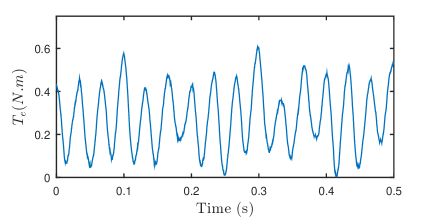
(a) Time evolution of $T_{e}$.

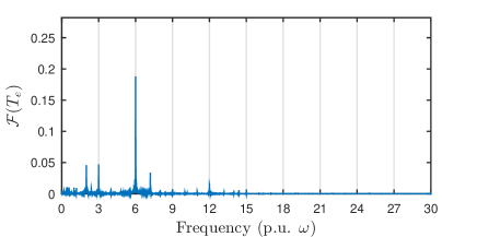
(b) Spectrum of $T_{e}$.

Figure 4: Electromagnetic torque $T_{e}$.

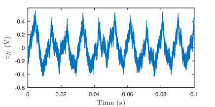
(a) Time evolution of $v_{N}$.

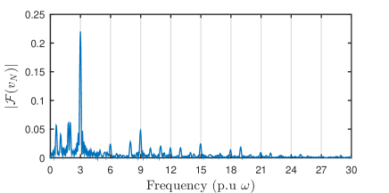
(b) Spectrum of $v_{N}$.

Figure 5: Potential $v_{N}$ of the star point.

VII-B Saturated model

The ripple caused by non-sinusoidal effects is usually small with respect to the rated values, and can be neglected in the model for control proposes. We therefore concentrate on the fundamental term $\overline{\mathcal{H}}^{DQ}_{m0\star}$ in the Fourrier expansion of the magnetic energy (LABEL:eqn:nonsin:fourrier:star); as in the unsaturated case, the rotor is symmetric with respect to the plane defined by the $D$-and $0$-axes, so $\overline{\mathcal{H}}^{DQ}_{m0\star}$ is even with respect to ${\lambda_{s}^{Q}}$ by (73). Following [4], we consider a perturbation of the unsaturated model (LABEL:eqn:linear:pmsm) in the form

$$\overline{\mathcal{H}}^{DQ}_{m0\star}({\lambda_{s}^{D}},{\lambda_{s}^{Q}})=\frac{1}{2}{\rm f}^{D}({\lambda_{s}^{D}}-\Phi_{M})+\frac{1}{2}{\rm f}^{Q}\bigl{(}{\lambda_{s}^{Q}}^{2}\bigr{)}$$ (177)

$$\qquad+\>\frac{1}{2}{\rm f}^{X}\bigl{(}{\lambda_{s}^{D}}-\Phi_{M},{\lambda_{s}^{Q}}^{2}\bigr{)},$$ (178)

where ${\rm f}^{D}$, ${\rm f}^{Q}$, ${\rm f}^{X}$ are polynomials of order at most 4,

$${\rm f}^{D}({\psi_{s}^{D}}) := \Gamma_{\!s}^{D}\Bigl{(}{\psi_{s}^{D}}^{2}+\frac{{\psi_{s}^{D}}^{3}}{6\phi_{1}^{D}}+\frac{{\psi_{s}^{D}}^{4}}{12{\phi_{2}^{D}}^{2}}\Bigr{)}$$

$${\rm f}^{Q}({\lambda_{s}^{Q}}^{2}) := \Gamma_{\!s}^{Q}\Bigl{(}{\lambda_{s}^{Q}}^{2}+\frac{{\lambda_{s}^{Q}}^{4}}{12{\phi_{1}^{Q}}^{2}}\Bigr{)}$$

$${\rm f}^{X}({\psi_{s}^{D}},{\lambda_{s}^{Q}}^{2}) := \Gamma_{\!s}^{D}\Bigl{(}\frac{{\psi_{s}^{D}}}{2\phi_{1}^{X}}+\frac{{\psi_{s}^{D}}^{2}}{{\phi_{2}^{X}}^{2}}\Bigr{)}{\lambda_{s}^{Q}}^{2},$$

and ${\psi_{s}^{D}}:={\lambda_{s}^{D}}-\Phi_{M}$. The 7 parameters $\Gamma_{\!s}^{D}$, $\Gamma_{\!s}^{Q}$, $\phi_{1}^{D}$, $\phi_{2}^{D}$, $\phi_{1}^{Q}$, $\phi_{1}^{X}$ and $\phi_{2}^{X}$ have to be determined experimentally. This model can be seen as a fourth-order Taylor expansion of the true energy function, whereas the unsaturated model is just a second-order expansion.

The 7 parameters were experimentally identified with signal injection, see [4] for details about the procedure; the values are given in table II. Fig. 6 illustrate the good agreement between the model and the experimental data; the saturation effects are clearly visible, though this high-end motor exhibits little saturation compared to more standard motors.

VII-C The role of magnetic saturation for sensorless control

In sensorless control, the actual control input in the model (168a)-(171a) is $v_{s}^{abc}$, or equivalently $v_{s}^{\alpha\beta}$, and the actual measurement is $\imath_{s}^{abc}$, or equivalently $\imath_{s}^{\alpha\beta}$. At zero velocity, there is a loss of observability, which makes the control problem more difficult in this zone. A fairly recent but now well-established method, called signal injection, to overcome this problem is to use an hybrid control law of the form

$$v_{s}^{\alpha\beta} := \bar{v_{s}}^{\alpha\beta}+\widetilde{v_{s}}^{\alpha\beta}f(t),$$

where $\bar{v_{s}}^{\alpha\beta}$ and $\widetilde{v_{s}}^{\alpha\beta}$ are “slowly-varying” inputs, and $f(t)$ is a “high-frequency” periodic signal. Following the analysis based on second-order averaging of [16, 4], the net effect of this signal injection is to make available for use in the control law the “virtual output”

$$\widetilde{\imath_{s}}^{\alpha\beta} := \partial_{\lambda_{s}^{DQ}}\imath_{s}^{\alpha\beta}\cdot\mathcal{R}_{2}(-\theta)\widetilde{v_{s}}^{\alpha\beta}$$

$$= \partial_{\lambda_{s}^{DQ}}\bigl{(}\mathcal{R}_{2}(\theta)\nabla_{\lambda_{s}^{DQ}}\mathcal{H}^{DQ}(\lambda_{s}^{DQ})\bigr{)}\cdot\mathcal{R}_{2}(-\theta)\widetilde{v_{s}}^{\alpha\beta}$$

$$= \mathcal{R}_{2}(\theta)\partial_{\lambda_{s}^{DQ}}\nabla_{\lambda_{s}^{DQ}}\mathcal{H}^{DQ}(\lambda_{s}^{DQ})\mathcal{R}_{2}(-\theta)\widetilde{v_{s}}^{\alpha\beta},$$

where

$$S(\theta,\lambda_{s}^{DQ}) := \mathcal{R}_{2}(\theta)\partial_{\lambda_{s}^{DQ}}\nabla_{\lambda_{s}^{DQ}}\mathcal{H}^{DQ}(\lambda_{s}^{DQ})\mathcal{R}_{2}(-\theta)$$

is the so-called saliency matrix; thanks to this extra output, the observability problem disappears provided $S$ effectively depends on $\theta$.

For an unsaturated PMSM described by (LABEL:eqn:linear:pmsm), the saliency matrix boils down to

$$\mathcal{R}_{2}(\theta)\begin{pmatrix}\Gamma_{\!s}^{D}&0\\ 0&\Gamma_{\!s}^{Q}\end{pmatrix}\mathcal{R}_{2}(-\theta).$$

If the motor has little geometric saliency, as is the case for an SPMSM, $\Gamma_{\!s}^{D}\approx\Gamma_{\!s}^{Q}$; this implies $S\approx\Gamma_{\!s}^{D}I$, i.e., $S$ does not depend on $\theta$. Ignoring magnetic saturation would lead to the wrong conclusion that such a motor cannot be controlled by signal injection. But when saturation is taken into account through (LABEL:eqn:nonlinear:pmsm), $S$ will in general depend on $\theta$ thanks in particular to the off-diagonal terms of $\partial_{\lambda_{s}^{DQ}}\nabla_{\lambda_{s}^{DQ}}\mathcal{H}^{DQ}$. Correctly describing saturation is thus paramount for operation at low velocity, which is experimentally confirmed, see e.g. [4].

Figure 6: Experimental current-flux relations $\imath_{s}^{D}({\lambda_{s}^{D}}-\Phi_{M},0)$ (—) and $\imath_{s}^{Q}(0,{\lambda_{s}^{Q}})$ (—) vs model (– –).

Table II: Estimated parameters

Parameters of ${\rm f}^{D}$		Parameters of ${\rm f}^{Q}$		Parameters of ${\rm f}^{X}$
$\frac{1}{\Gamma_{\!s}^{D}}$	$8.8\text{\,}\mathrm{mH}$	$\frac{1}{\Gamma_{\!s}^{Q}}$	$7.7\text{\,}\mathrm{mH}$
$\phi_{1}^{D}$	$0.533\text{\,}\mathrm{Wb}$	$\phi_{1}^{Q}$	$0.228\text{\,}\mathrm{Wb}$	$\phi_{1}^{x}$	$0.116\text{\,}\mathrm{Wb}$
$\phi_{2}^{D}$	$0.200\text{\,}\mathrm{Wb}$			$\phi_{2}^{x}$	$0.111\text{\,}\mathrm{Wb}$

section VIII Conclusion

We have proposed an approach to modeling of AC motors entirely based on analytical mechanics, and taken into account geometric symmetries and connection constraints in the energy function. The approach is well-suited to handle magnetic saturation, which is paramount in the design of sensorless control laws are very low speed. In particular, it justifies the fact that star-connected saturated models can be expressed in the $DQ$ (or $dq$) frame, which is not obvious though usually taken for granted in the literature.

A further step in modeling would be to incorporate some hysteresis effects, which seem to be the next major phenomenon in AC motors without permanent magnets (SynRM and IM) once magnetic saturation has been taken into account.

References

• [1] Y. Li, Z. Zhu, D. Howe, C. Bingham, and D. Stone, “Improved rotor-position estimation by signal injection in brushless AC motors, accounting for cross-coupling magnetic saturation,” IEEE Transactions on Industry Applications, vol. 45, pp. 1843–1850, 2009.
• [2] P. Sergeant, F. De Belie, and J. Melkebeek, “Effect of rotor geometry and magnetic saturation in sensorless control of PM synchronous machines,” IEEE Trans. Magnetics, vol. 45, no. 3, pp. 1756–1759, 2009.
• [3] N. Bianchi, E. Fornasiero, and S. Bolognani, “Effect of stator and rotor saturation on sensorless rotor position detection,” in IEEE Energy Conversion Congress and Exposition, 2011, pp. 1528–1535.
• [4] A. K. Jebai, F. Malrait, P. Martin, and P. Rouchon, “Sensorless position estimation and control of permanent-magnet synchronous motors using a saturation model,” International Journal of Control, vol. 89, no. 3, pp. 535–549, 2016.
• [5] P. Vas, Sensorless Vector and Direct Torque Control, ser. Monographs in electrical and electronic engineering.   Oxford University Press, 1998.
• [6] P. Krause, O. Wasynczuk, S. Sudhoff, and S. Pekarek, Analysis of Electric Machinery and Drive Systems.   Wiley, 2013.
• [7] J. Chiasson, Modeling and High Performance Control of Electric Machines.   Wiley, 2005.
• [8] J. Holtz and L. Springob, “Identification and compensation of torque ripple in high-precision permanent magnet motor drives,” IEEE Transactions on Industrial Electronics, vol. 43, no. 2, pp. 309–320, 1996.
• [9] V. Petrovic, R. Ortega, A. M. Stankovic, and G. Tadmor, “Design and implementation of an adaptive controller for torque ripple minimization in pm synchronous motors,” IEEE Transactions on Power Electronics, vol. 15, no. 5, pp. 871–880, 2000.
• [10] J. Melkebeek and J. Willems, “Reciprocity relations for the mutual inductances between orthogonal axis windings in saturated salient-pole machines,” IEEE Transactions on Industry Applications, vol. 26, no. 1, pp. 107–114, 1990.
• [11] D. White and H. Woodson, Electromechanical Energy Conversion.   Wiley, 1959.
• [12] D. Jeltsema and J. M. A. Scherpen, “Multidomain modeling of nonlinear networks and systems,” IEEE Control Systems Magazine, vol. 29, no. 4, pp. 28–59, 2009.
• [13] A. Jebai, P. Combes, F. Malrait, P. Martin, and P. Rouchon, “Energy-based modeling of electric motors,” in IEEE Conference on Decision and Control, 2014, pp. 6009–6016.
• [14] A. I. Lurie, Analytical mechanics, ser. Foundations of Engineering Mechanics.   Springer-Verlag, 2002, translated by A. Belyaev.
• [15] B. K. Bose, Modern Power Electronics and AC Drives.   Prentice Hall PTR, 2002.
• [16] P. Combes, A. K. Jebai, F. Malrait, P. Martin, and P. Rouchon, “Adding virtual measurements by signal injection,” in American Control Conference, 2016, pp. 999–1005.