A test field for Gaia

Abstract

Context. Gaia is a space mission currently measuring the five astrometric parameters as well as spectrophotometry of at least 1 billion stars to $G=20.7$ mag with unprecedented precision. The sixth parameter in phase space — radial velocity — is also measured thanks to medium-resolution spectroscopy being obtained for the 150 million brightest stars. During the commissioning phase, two fields, one around each ecliptic pole, have been repeatedly observed to assess and to improve the overall satellite performances as well as the associated reduction and analysis software. A ground-based photometric and spectroscopic survey was therefore initiated in 2007, and is still running in order to gather as much information as possible about the stars in these fields. This work is of particular interest to the validation of the Radial Velocity Spectrometer (RVS) outputs.

Aims. The paper presents the radial velocity measurements performed for the Southern targets in the 12 - 17 $R$ magnitude range on high- to mid-resolution spectra obtained with the GIRAFFE and UVES spectrographs.

Methods. Comparison of the South Ecliptic Pole (SEP) GIRAFFE data to spectroscopic templates observed with the HERMES (Mercator in La Palma, Spain) spectrograph allowed a first coarse characterisation of the 747 SEP targets. Radial velocities were then obtained by comparing the results of three different methods.

Results. In this paper we present an initial overview of the targets to be found in the 1-square-degree SEP region that was observed repeatedly by Gaia from its commissioning on. In our representative sample, we identified 1 galaxy, 6 LMC S-stars, 9 candidate chromospherically active stars, and confirmed the status of 18 LMC Carbon stars. A careful study of the 3471 epoch radial velocity measurements, led us to identify 145 RV constant stars with radial velocities varying by less than 1 $\mathrm{km}\,\mathrm{s}^{\mathrm{-1}}$. 78 stars show significant RV scatter, while nine stars show a composite spectrum. As expected the distribution of the RVs exhibits 2 main peaks corresponding to Galactic and LMC stars. By combining $[\mathrm{Fe/H}]$  and $\log g$  estimates, and RV determinations we identified 203 members of the LMC, while 51 more stars are candidate members.

Conclusions. This is the first systematic spectroscopic characterisation of faint stars located in the SEP field. During the coming years, we plan to continue our survey and gather additional high- and mid-resolution data to better constrain our knowledge on key reference targets for Gaia.

1 Introduction

Gaia, ESA’s astrometric satellite mission, was launched on December 19th, 2013. It is currently obtaining the astrometry of more than 1 billion stars with unprecedented precision and with the ultimate goal of creating a 3-D map of the stellar component of our Galaxy and its surroundings. The mission will nominally last 5 years and is based on the principles of the earlier and successful Hipparcos mission.

To achieve its goals, Gaia measures the five components of the six dimensional phase space (coordinates, parallax, and 2-D proper motion) for all objects with $G$ (i.e., broad-band Gaia magnitude, Jordi et al. 2010) ranging from $3$ to $20.7$ mag (Solar System bodies, $10^{\rm{9}}$ stars as well as several million galaxies and quasars, see Robin et al. 2012). The sixth parameter (i.e., radial velocity) is derived for the stars up to $G_{\mathrm{RVS}}$ $\sim 16.2$ mag (i.e., Radial Velocity Spectrometer - RVS - narrow band magnitude, see Katz et al. 2004; Cropper & Katz 2011). Final parallax errors as small as $80$ $\mathrm{\mu as}$  are expected (Luri et al. 2014). In addition to accurate astrometry (Prusti 2010), Gaia will provide dispersed photometry (an expected average of 70 measurements per target) in 2 wavelength domains (Blue Photometer, BP, and Red Photometer, RP) with a total wavelength coverage from $330$ to $1050$ nm and an average resolving power $\mathcal{R}\sim 20$ (Jordi et al. 2010). The brighter stars will further be observed on average 40 times during the mission at a higher resolving power $\mathcal{R}\sim 11\,500$ by means of the RVS, in a spectral domain ranging from $845$ to $872$ nm known as the region of the near-IR Ca ii triplet and of the higher members of the Paschen series. Gaia will therefore also classify the objects it observes, which for stars implies the determination of astrophysical parameters (APs). For the latest up-to-date science performance values, the reader may refer to the official Gaia web page and to the first companion paper of the Gaia Data Release 1 (GDR1, Gaia Collaboration et al. 2016).

Unlike Hipparcos, Gaia does not use an input catalogue but scans the whole sky to observe all objects up to magnitude $G\sim 20.7$. To achieve this, it follows a scan law called the Nominal Scan Law (NSL) designed to optimise astrometric accuracy, sky coverage, and uniformity taking into account the selected orbit as well as other mission-related technical aspects (Lindegren & Bastian 2011). In addition to the NSL, in order to perform the initial calibration of the instruments and to verify the high-precision astrometric performances during the commissioning phase, an Ecliptic Pole Scanning Law (EPSL) was introduced. This law allows, from the very beginning of the mission, to observe many times during a short period of time a 1-square-degree field centred on each ecliptic pole (EP), in the Southern (SEP) and Northern (NEP) hemispheres.

Because these are test fields, there is a continuous effort to collect as much knowledge as possible about them. While all literature data available for the bright stars were included in the Initial Gaia Source List (IGSL, Smart & Nicastro 2014), a photometric survey was initiated in 2007 with the MEGACAM facility on the Canadian French Hawaii Telescope for the North ecliptic pole and with the WFI imager on the ESO 2.2-m telescope for the South ecliptic pole. The aims were to collect reference data and to characterise the faintest stars of the EP fields between $R$ magnitudes 13 and 23.

In a similar effort, the acquisition of reference radial velocity measurements for standard stars with the goal to support, and to calibrate the RVS is carried out for stars brighter than $V=11$ (see e.g., Crifo et al. 2010; Jasniewicz et al. 2011; Soubiran et al. 2013). Other RV catalogues like the Geneva-Copenhagen survey (GCS, Nordström et al. 2004) or RAVE (The Radial Velocity Experiment, Siebert et al. 2011; Kordopatis et al. 2013) are used for large scale verification purposes. However, they also mainly include bright stars in the SEP, which does not permit to characterise the faint-end radial velocity performance of the instrument. Therefore, in the framework of the preparation of the Gaia Ecliptic Pole Catalogue (GEPC, Altmann 2013), 747 SEP targets with $V$ magnitudes ranging from $13$ to $18$ were repeatedly observed (see Sect. 2) at high- to mid-spectral resolution with the GIRAFFE and/or UVES spectrographs, as well as with the Wide Field Imager on the MPIA 2.2-m telescope (ESO) in the $B$, $V$, $R$, $I$ photometric bands. The main purpose is to characterise in as great detail as possible all the stars that were observed by deriving their radial velocity, astrophysical parameters, and chemical composition.

The present study deals with the determination of the radial velocities on spectra obtained with two spectrographs, in three different wavelength ranges, and at three different spectral resolutions. Because each RV determination method (David et al. 2014) is sensitive in a different way to instrumental, template mismatch or line blending effects, we chose to adopt a multi-method RV determination approach and to confront the results of the 3 independent methods.

This paper is organised as follows: the observations are described in Sect. 2, while Sect. 3 explains how we perform a first characterisation of the targets. Section 4 outlines the three methods we use to derive the radial velocities. The results are compared and analysed in Sect. 5, then discussed in Sect. 6, and summarised in Sect. 7.

Figure 1: South Ecliptic Pole coverage: Six different FLAMES pointings (circular shaded areas) were used. Symbol size is proportional to the brightness. Confirmed LMC stars (Sect. 6.3) are represented by filled symbols, while other targets are pictured with open symbols. UVES targets are shown by red triangles. Carbon and S stars are marked by green squares and blue diamonds (Sect. 6.4), respectively, while the galaxy in our sample is located by a yellow pentagon.

longtablerrrrlrrrrr $BVRI$ photometry of South ecliptic pole stars with UVES and/or GIRAFFE data: The table lists the 747 observed targets with their 2MASS ID, their sequence number in the first version of the GEPC, and their coordinates (right ascension and declination). The coordinates were cross-matched with the OGLE SEP catalogue of variable stars (Soszyński et al. 2012). For the 218 matches found within $1$ arcsec, we also provide the OGLE ID as well as the angular distance from the tabulated coordinates. In the four last columns, we further give the $BVRI$ photometry obtained in 2007 and 2009 at the ESO-La Silla observatory in Chile with the 2.2-m telescope and the WFI instrument. (The complete version of the table will be made available at the CDS.)
EPOCH 2000
2MASS ID EID RA DEC OGLE ID Ang. Dist. $B$ $V$ $R$ $I$
(deg) (deg) (arcsec) (mag) (mag) (mag) (mag)
continued.
EPOCH 2000
2MASS ID EID RA DEC OGLE ID Ang. Dist. $B$ $V$ $R$ $I$
(deg) (deg) (arcsec) (mag) (mag) (mag) (mag)
J05560865-6621388 21404 89.036083 -66.360722 16.64 15.96 15.58 15.40
J05560908-6620343 21498 89.037875 -66.342833 – – – –
J05561590-6627158 22969 89.066250 -66.454361 LMC563.10.14 0.200 18.30 16.33 15.06 13.98
J05561592-6626530 22979 89.066333 -66.448056 18.01 16.61 15.92 15.20

2 Data sample

2.1 Spectroscopic observations

The spectra were obtained with ESO’s VLT UT2 and the FLAMES facility (Pasquini et al. 2002) in Medusa combined mode. In this mode, up to 132 fibres can be located on objects feeding the GIRAFFE multi-object spectrograph, while up to 8 fibres can be placed and directed to the red arm of UVES. The field of view of FLAMES is 25 arcmin in diameter. The facility has two different fibre plates, so that while one is being observed, the other one gets configured. A small part of the field is obstructed by the VLT guide probe. The object positioning was made using the FPOSS software, dedicated to set up FLAMES. A number of fibres fed into GIRAFFE and UVES are reserved for measuring the sky background.

The GIRAFFE spectrograph offers two suites of gratings, medium resolution (”LR”, with a longer wavelength range) and high-resolution (”HR”, with a smaller range). We chose two gratings: HR21, which has a resolving power of $\mathcal{R}$$=16\,200$ and a wavelength range from $848.4$ nm to $900.1$ nm, and the LR2 which has a spectral domain ranging from $396.4$ nm to $456.7$ nm with $\mathcal{R}$$=6\,400$. For the UVES stars, we also covered the Gaia range by using the $860$ nm setup (RED860), which uses a mosaic of 2 CCDs with a resolving power of $\mathcal{R}$$=47\,000$. The Lower (RED–L) and Upper (RED–U) CCD spectra are ranging from $673$ to $853$ nm and from $865$ to $1060$ nm, respectively. UVES RED860 therefore features a gap from $853$ to $865$ nm, right in the middle of the Gaia RVS range. For this reason, we reobserved most UVES stars with the HR21 grating as well.

The HR21 setup completely encompasses the wavelength domain of the RVS aboard Gaia, which is the reason why this grating was chosen. It mainly contains the important Ca ii triplet (at $849.8$ nm, $854.2$ nm, and $866.2$ nm), which is well suited for RV determination, as demonstrated by the RAVE survey, and which is also used for the estimation of metallicity (e.g., Carrera et al. 2007, 2013). It furthermore includes the higher members of the Paschen series of hydrogen (e.g., Andrillat et al. 1995; Frémat et al. 1996) that become stronger in A- and B-type stars.

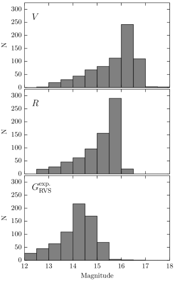
Figure 2: Magnitude distribution of the sample: Distribution of $V$, $R$, and $G^{\mathrm{exp.}}_{\rm{RVS}}$ magnitudes of the stars observed with the GIRAFFE and UVES spectrographs. $G^{\mathrm{exp.}}_{\mathrm{RVS}}$ is the expected RVS narrow band magnitude that was estimated from the relations provided by Jordi et al. (2010).

To ease the exposure time computation and to carry-out the observations in the most efficient way, the GIRAFFE stars were selected randomly within two magnitude bins (the magnitude distributions of the sample are provided in Fig. 2), one brighter than $R\sim 15$ mag, and one ranging from $R\sim 15\leavevmode\nobreak\ \mathrm{to}\leavevmode\nobreak\ 16.5$ mag, which approximately gives the lower brightness limit for the RVS instrument of Gaia. The UVES stars were chosen to be brighter than the GIRAFFE stars belonging to the same exposure, since the higher resolution of this instrument demands more light to reach a sufficiently high SNR level. The FPOSS positioning software allows for several modes of fibre allocation. Because in this magnitude range our field was not crowded, the allocation mode was not critical. Usually we could allocate fibres to most target stars, with some fibres to spare. This especially holds true for those exposures in which the brighter stars were covered. Nonetheless fibre conflicts did occur, and thus not all of the selected stars could be observed.

We used six different pointings (see Fig. 1). As some of these circular fields do overlap, there are a number of stars present in more than one pointing. The stars within a field and within a magnitude bin were selected randomly, in such a way as to ensure a maximum of targets being allocated with fibres. This further also ensures an unbiased stellar sample (except for the magnitude limits), which is representative of the SEP-field in the aforementioned magnitude ranges. In total, 747 objects have been observed and listed in Table 1 with their 2MASS ID and their sequence number in the first version of the GEPC (EID). For the sake of convenience, we will hereafter only designate the stars by their EID. Table 1 further provides the right ascension and the declination, which were cross-matched with the OGLE SEP catalogue of variable stars (Soszyński et al. 2012). We found 218 matches within $1$ arcsec, and provide their OGLE ID as well as the angular distance from the tabulated coordinates in the 2 next columns of the same table.

The observations were done over 4 semesters (ESO P82, 84, 86, 88) in service mode. ESO-Observing blocks are generally restricted to last not more than 1 hour in total, therefore the observations were split into several exposures. Table 1 is an overview of the observations. It gives the observing block ID (OB), the modified Julian date (MJD), GIRAFFE setup, plate number, exposure time, period of observation, pointing direction (see also Fig. 1), and median per sample SNR value, respectively.

Table 1: GIRAFFE observations log (The complete version of the table will be made available at the CDS.)

OB ID	MJD	Setup	Plate	texp	Period	Pointing	SNR
				(s)
389193	55185.34904	LR2	1	2000	P84	P1	9
389179	55202.23191	HR21	2	2700	P84	P3	7
389178	55203.31727	HR21	2	2200	P84	P3	13

2.1.1 Data reduction

The raw frames of the GIRAFFE observations have been reduced by us using the ESO GIRAFFE pipeline (release 2.12.1). Before running the localisation recipe, automatic identification of missing fibres has been performed on the raw flat-field frames and fed as input to the recipe. One-dimensional spectra were extracted, for both flat-field and science frames, using the optimal extraction method.

Sky lines are spread over the HR21 wavelength domain, and need to be removed. To do that we adopted a methodology inspired by the one described in Battaglia et al. (2008). We applied k-sigma clipping to scale the sky lines of the median sky spectrum to those extracted from the object spectrum. The rescaled median sky spectrum was then subtracted from the object spectrum and the result smoothed. When no sky fibres were available, we used the median sky of the closest exposure. For the final continuum normalisation or correction, we proceeded as explained in Sect. 4.1.

It is worth adding that we do not shift the object spectrum to place it in the framework of the sky lines as is done by Battaglia et al. (2008). The clipped out sky lines were rather used to evaluate the median shift and its dispersion by comparison to the median sky lines of a given night ($\mathrm{MJD}=55\,271.13419$, see Table 1). In this way, the median sky line shift obtained for the dataset is $+0.19$ $\mathrm{km}\,\mathrm{s}^{\mathrm{-1}}$ with a dispersion (measured as half the interquantile range from 15.87% to 84.13%, see eq.19 in David et al. 2014) of $0.25$ $\mathrm{km}\,\mathrm{s}^{\mathrm{-1}}$ (P84 over 973 spectra: $0.13\pm 0.24$ $\mathrm{km}\,\mathrm{s}^{\mathrm{-1}}$; P86 over 1065 spectra: $0.25\pm 0.30$ $\mathrm{km}\,\mathrm{s}^{\mathrm{-1}}$; P88 over 47 spectra: $-0.16\pm 0.24$ $\mathrm{km}\,\mathrm{s}^{\mathrm{-1}}$). This definition for dispersion will be used throughout the text. The scatter reflects the mean precision and stability level of the wavelength calibration over the 3 years of observation.

Additionally there are a few telluric-lines present at the very red edge of the same wavelength range (mainly from $890$ to $900$ nm) that we cross-correlated to a synthetic spectrum of the Earth atmosphere transmission generated by the TAPAS web server (Bertaux et al. 2014). The median shift of the telluric-lines over the 3 periods we observed is $+0.49\pm 0.74$ $\mathrm{km}\,\mathrm{s}^{\mathrm{-1}}$, which is consistent with the value obtained for each one individually (P84: $+0.52\pm 0.67$ $\mathrm{km}\,\mathrm{s}^{\mathrm{-1}}$; P86: $+0.47\pm 0.81$ $\mathrm{km}\,\mathrm{s}^{\mathrm{-1}}$; P88: $+0.26\pm 0.40$ $\mathrm{km}\,\mathrm{s}^{\mathrm{-1}}$).

UVES spectra were reduced with the UVES pipeline (Ballester et al. 2000; Modigliani et al. 2004) which performs bias and flat-field correction (this last step also corrects for the different fibre transmission), spectra tracing, optimal extraction, and wavelength calibration. We generally used two of the eight available UVES fibres to obtain sky spectra. After comparing the sky spectra, to verify that they were compatible with each other and showed no artifacts or clear contamination from faint stars, we created a master sky spectrum as an average of the two sky spectra, and subtracted it from all scientific spectra of the same pointing. The sky-subtracted UVES spectra were normalised by their continuum shape with low order polynomials. The telluric-line shifts relative to the TAPAS data were then measured by using the same approach as for GIRAFFE data over all 3 observed periods, which provided a median shift of $-0.64\pm 0.45$ $\mathrm{km}\,\mathrm{s}^{\mathrm{-1}}$ (P84 over 60 spectra: $-0.68\pm 0.47$ $\mathrm{km}\,\mathrm{s}^{\mathrm{-1}}$; P86 over 119 spectra: $-0.57\pm 0.43$ $\mathrm{km}\,\mathrm{s}^{\mathrm{-1}}$; P88 over 34 spectra: $-0.76\pm 0.42$ $\mathrm{km}\,\mathrm{s}^{\mathrm{-1}}$). When considering RED–L and RED–U measurements independently, the median of the differences, $\overline{\Delta\mathrm{RV}_{\mathrm{UL}}}=\mathrm{RV}_{\mathrm{U}}-\mathrm{RV}_{\mathrm{L}}$, is $0.08\pm 0.19$ $\mathrm{km}\,\mathrm{s}^{\mathrm{-1}}$.

Because the telluric-lines are well distributed over the observed wavelength domain, and that we also use ESO archive data (see Sect. 5.2) spread over a long period of time, all RV values measured on the UVES spectra were brought into the framework of the Earth atmosphere absorption lines.

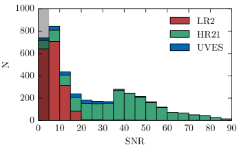
Figure 3: Stacked histograms of the SNR of all observations: Distribution (bin width = 5) of the SNR per sample in the GIRAFFE and UVES spectra. Spectra with SNR $<$ 5 (gray shaded region) have only been considered for stellar classification to obtain a co-added spectrum.

As can be seen in the stacked histogram of Fig. 3, due to the nature of the SEP stellar population mainly made of cooler stars, HR21 observations generally achieved higher SNR. In total, 4129 spectra were reduced from which 3471 (190 UVES, 1167 LR2, 2114 HR21) had an $\mathrm{SNR}\geq 5$. Therefore, while 747 targets have been observed, only 724 have epoch spectra of sufficiently high quality to derive epoch radial velocities and discuss their variability. Despite of this, we included the lower quality data to produce the co-added spectra we use to determine the best template as explained in Sect. 4.1.2.

2.2 Photometric observations

The photometric data were obtained in 2007 and 2009 at the ESO-La Silla observatory in Chile with the 2.2-m telescope and the WFI instrument. The November 2007 data was incomplete and did not allow for photometric calibration. Both issues were remedied with the second run in January 2009. The data was reduced using MIDAS and the MPIAphot (Meisenheimer & Röser 1986) suite. Calibration was done using Landolt standards (Landolt 1992). While the photometry and astrometry of the SEP and NEP will be published in a separate paper, we provide the $BVRI$ magnitudes in the 4 last columns of Table 1 as these values were used to initiate the template optimisation procedure (Sect. 4.1.2) as well as to estimate the expected brightness coverage in terms of $G_{\mathrm{RVS}}$  magnitude (see conversion relations in Jordi et al. 2010). $R$, $I$, and expected $G_{\mathrm{RVS}}$ magnitude distributions are plotted in Fig. 2.

3 First insight into the data using HERMES spectra

Because the targets were selected at random and that there is not much information available on such faint stars, we decided to perform a preliminary target characterisation based on the use of HERMES reference observations.

Since the beginning of the exploitation of the high-resolution HERMES spectrograph (Raskin et al. 2011) in 2009 on the Mercator telescope (Roque de los Muchachos Observatory on La Palma, Canary Islands, Spain), a large volume of data has been acquired. One of the observing projects is running without interruption since the beginning of operations (late 2009). It is conceived as a fill-in program (PI: P. Royer) and consists in the acquisition of high SNR data across the HR diagram. We performed a first empirical classification of the GIRAFFE data by systematically comparing the SEP spectra to a subsample of the HERMES library. Our sample of HERMES template stars was built by selecting 641 stars having a spectrum with $\mathrm{SNR}>100$, with known astrophysical parameters ($T_{\mathrm{eff}}$  and $\log g$), and mainly single lined. The $\log g$  vs $T_{\mathrm{eff}}$  coverage of the library is plotted in Fig. 4, with a colour code that matches the published $[\mathrm{Fe/H}]$. Each spectrum was convolved with a Gaussian LSF to match the spectroscopic resolution of the LR2 and HR21 settings, then compared to the available GIRAFFE spectra by adopting a cross-correlation technique. These comparisons have been performed in the 2 settings independently, in order to potentially detect binary components with different colours. The identification and parameters corresponding to the most similar HERMES spectrum (i.e., with the highest correlation peak) are provided in Table 3 in the following order: star’s EID, explored GIRAFFE Setup (GS), and for each GS the ID of the HERMES reference target with the closest spectrum, its $T_{\mathrm{eff}}$, $\log g$, $[\mathrm{Fe/H}]$, and $\varv\sin{i}$. The origin of the spectral type and parameters are given between brackets. In cases where no literature reference is provided for the spectral type, the classification is the one found in the basic information tab in the Simbad database (CDS), while the same situation for the astrophysical parameters means that the values were estimated using the available Strömgren photometry as well as the Moon & Dworetsky (1985) calibration updated by Napiwotzki (1997). We observe that LR2 and HR21 $T_{\mathrm{eff}}$  determinations are generally in good agreement, as the median difference and dispersion are of the order of $244\pm 236$ K. When the $T_{\mathrm{eff}}$  in LR2 and HR21 wavelength domains are different by more than $1000$ K, the target is highlighted in bold font.

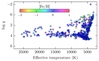
Figure 4: Parameter space coverage of the HERMES reference spectra: $\log g$  is reported as a function of $T_{\mathrm{eff}}$, while a colour code is used to picture the published $[\mathrm{Fe/H}]$. When $[\mathrm{Fe/H}]$  is unknown, the value is assumed to be zero.

longtablerlllcrrrcrc SEP targets and characteristics of the corresponding closest HERMES spectrum: The table provides the star’s EID, explored GIRAFFE Setup (GS), and for each GS the ID of the HERMES reference target with the closest spectrum, its $T_{\mathrm{eff}}$, $\log g$, $[\mathrm{Fe/H}]$, and $\varv\sin{i}$. The origin of the spectral type and parameters are given between brackets and in the table footer. When no literature reference is provided for the spectral type, the classification is the one found in the basic information tab in the Simbad database (CDS), while the same situation for the astrophysical parameters means that the values were estimated using the available Strömgren photometry as well as the Moon & Dworetsky (1985) calibration updated by Napiwotzki (1997). When the $T_{\mathrm{eff}}$  in LR2 and HR21 wavelength domains are different by more than $1000$ K, the target is highlighted in bold font. (The complete version of the table will be made available at the CDS.)
Closest HERMES spectrum
EID GS ID Sp. Type $T_{\mathrm{eff}}$ $\log g$ $[\mathrm{Fe/H}]$ $\varv\sin{i}$
continued.
Closest HERMES spectrum
EID GS ID Sp. Type $T_{\mathrm{eff}}$ $\log g$ $[\mathrm{Fe/H}]$ $\varv\sin{i}$
21404 LR2 HD 18757 G1.5 V (1) 5741 4.30 -0.25 (2) 0 (2)
HR21 HD 18757 G1.5 V (1) 5741 4.30 -0.25 (2) 0 (2)
21498 LR2 HD 115604 F3III (3) 6855 3.40 0.18 (4) 0 (4)
HR21 HD 23230 F5IIvar (25) 6675 2.00 0.04 (55) 44 (48)
22969 LR2 HIP 86162 M3 (5) 3583 4.86 0.00 (30)
HR21 HD 92839 C 5 II (36) 3623 4.80 -0.10 (24)
22979 LR2 HD 20618 G8IV (6) 5093 3.20 (4) 2 (4)
HR21 HD 159222 G1 V (1) 5788 4.25 (1) 3 (14)
23240 LR2 HD 42995 M3III (7) 3600 1.50 0.04 (8)
(1) Gray et al. (2003); (2) Mishenina et al. (2012); (3) Cenarro et al. (2009); (4) Massarotti et al. (2008); (5) Rojas-Ayala et al. (2012); (6) Harlan (1969); (7) Eggen (1962); (8) Mallik (1998); (9) Cowley et al. (1967); (10) Lee et al. (2011); (11) Prugniel et al. (2011); (12) Tabernero et al. (2012); (13) Allende Prieto et al. (2004); (14) Martínez-Arnáiz et al. (2010); (15) Sozzetti et al. (2009); (16) Reddy et al. (2003); (17) Houdebine (2010); (18) Fehrenbach (1961); (19) Ake (1979); (20) Smith & Lambert (1986); (21) Balachandran (1990); (22) Schröder et al. (2009); (23) Bruntt et al. (2012); (24) Frasca et al. (2009); (25) Griffin & Redman (1960); (26) Venn (1995); (27) Afşar et al. (2012); (28) Royer et al. (2007); (29) Morgan & Keenan (1973); (30) Soubiran et al. (2008); (31) Kang et al. (2011); (32) Molnar (1972); (33) Bailey & Landstreet (2013); (34) Kővári et al. (2007); (35) Luck & Lambert (2011); (36) Richer (1971); (37) Casagrande et al. (2011); (38) Montes et al. (2001); (39) Takeda (2007); (40) White et al. (2007); (41) Lesh (1968); (42) Huang et al. (2010); (43) Abt et al. (2002); (44) Boesgaard et al. (2001); (45) Takeda et al. (2005); (46) Thygesen et al. (2012); (47) Parsons & Ake (1998); (48) Uesugi & Fukuda (1970); (49) Koleva & Vazdekis (2012); (50) Bidelman (1951); (51) Hollek et al. (2011); (52) Eggen (1958); (53) Butler et al. (2006); (54) Luck & Bond (1991); (55) Luck & Wepfer (1995); (56) Ghezzi et al. (2010); (57) Sheffield et al. (2012); (58) Heard (1956); (59) Smith & Lambert (1990); (61) Fernandez-Villacanas et al. (1990); (62) Gray et al. (2006); (63) Hill (1995); (64) McWilliam (1990); (65) Edwards (1976); (66) Cowley et al. (1969); (67) Gielen et al. (2011); (68) Kraft (1960); (69) Moro-Martín et al. (2007); (70) Renson & Manfroid (2009); (71) Gratton et al. (1996); (72) Barry (1970); (73) Thorén & Feltzing (2000); (74) Bidelman (1957); (75) Balachandran et al. (2000); (76) Royer et al. (2002); (77) Keenan (1954); (78) Conti & Leep (1974); (79) Gray et al. (2001); (80) Cayrel et al. (1988); (81) Feltzing & Gustafsson (1998).

4 RV determination methods

We chose to adopt a multi-method approach based on the confrontation and combination of three independent RV determination procedures described in the following subsections.

4.1 Pearson correlation

The correlation of observed spectra with theoretical ones is performed by computing the Pearson correlation coefficient (David et al. 2014, and references therein) for different radial velocity shifts. To derive the star’s RV, we have reduced the step around the top of the Pearson Correlation Function (PCF) to 1 $\mathrm{km}\,\mathrm{s}^{\mathrm{-1}}$, then we combined the solution of 2 parabolic fits through 3 and 4 points taken on both sides of the maximum as described in David & Verschueren (1995). All the data manipulation, such as Doppler shifting and wavelength resampling, is applied on the template. Intrinsic errors on RV are deduced from the maximum-likelihood theory (Zucker 2003). We used a Fortran procedure which we named PCOR (Pearson Correlation) to perform these operations. To reduce the impact of possible mismatches at the spectra edges (e.g., due to normalisation) as well as to limit the blends with telluric lines, the correlation was computed in wavelength domains that exclude such features. In practice, we therefore only considered the spectral ranges listed in Table 2 with their corresponding instrument and observing mode/region, as well as their beginning ($\lambda_{\mathrm{beg.}}$), and end ($\lambda_{\mathrm{end}}$) wavelengths. In the case of the UVES data and for further comparisons with the 2 other methods, the radial velocity we kept is the median over the 5 available domains after correction of the telluric line shift and after having filtered out potential outliers thanks to Chauvenet’s criterion. For information purposes, we note that if a separate value for the UVES RED–L and RED–U spectra is computed, we obtain a median difference, $\overline{\Delta\mathrm{RV}_{\mathrm{UL}}}=\mathrm{RV}_{\mathrm{U}}-\mathrm{RV}_{\mathrm{L}}$, between both estimates of $0.14\pm 0.26$ $\mathrm{km}\,\mathrm{s}^{\mathrm{-1}}$ (where the error is the dispersion obtained for 158 spectra).

Table 2: Wavelength ranges taken into account by the PCOR (Pearson Correlation) procedure while deriving the stellar RVs

Spectrograph–region	$\lambda_{\mathrm{beg.}}$	$\lambda_{\mathrm{end}}$
	(nm)	(nm)
GIRAFFE–LR2	400.	450.
GIRAFFE–HR21	849.	875.
UVES–REDL	676.1	686.0
	694.0	708.0
	737.4	756.4
	773.5	811.3
UVES–REDU	868.0	889.0

Besides random and calibration errors, one possible source of systematic error on the measurement of RVs is the mismatch between the observations and the synthetic spectra used to construct the templates. The main mismatch problems originate from the use of inappropriate stellar atmosphere parameters, the application of inappropriate line broadening to account for the instrumental LSF or for stellar rotation, as well as imperfect or inconsistent (compared to the template) continuum normalisation of the observations. In order to reduce the impact of these errors, we adopted different spectral libraries that cover as closely as possible the expected range of atmospheric parameters, and applied a multi-step RV determination aimed to iteratively improve the choice and construction of the template spectrum.

4.1.1 Synthetic spectra libraries

Depending on the effective temperature range, different publicly available libraries of spectra were considered. To represent stars cooler than 3500 K, we adopted the BT-Settl PHOENIX grid from Rajpurohit et al. (2013). From 3500 K to 5500 K, the models computed by Coelho et al. (2005) were taken, while from 5500 K to 15000 K, MARCS (Gustafsson et al. 2008) and ATLAS (Castelli & Kurucz 2004) model spectra were downloaded from the Pollux database (Palacios et al. 2010). For higher effective temperatures, we used the BSTAR flux grids computed by Lanz & Hubeny (2007). All these 4593 spectra were convolved with a Gaussian instrument profile at the appropriate spectral resolution.

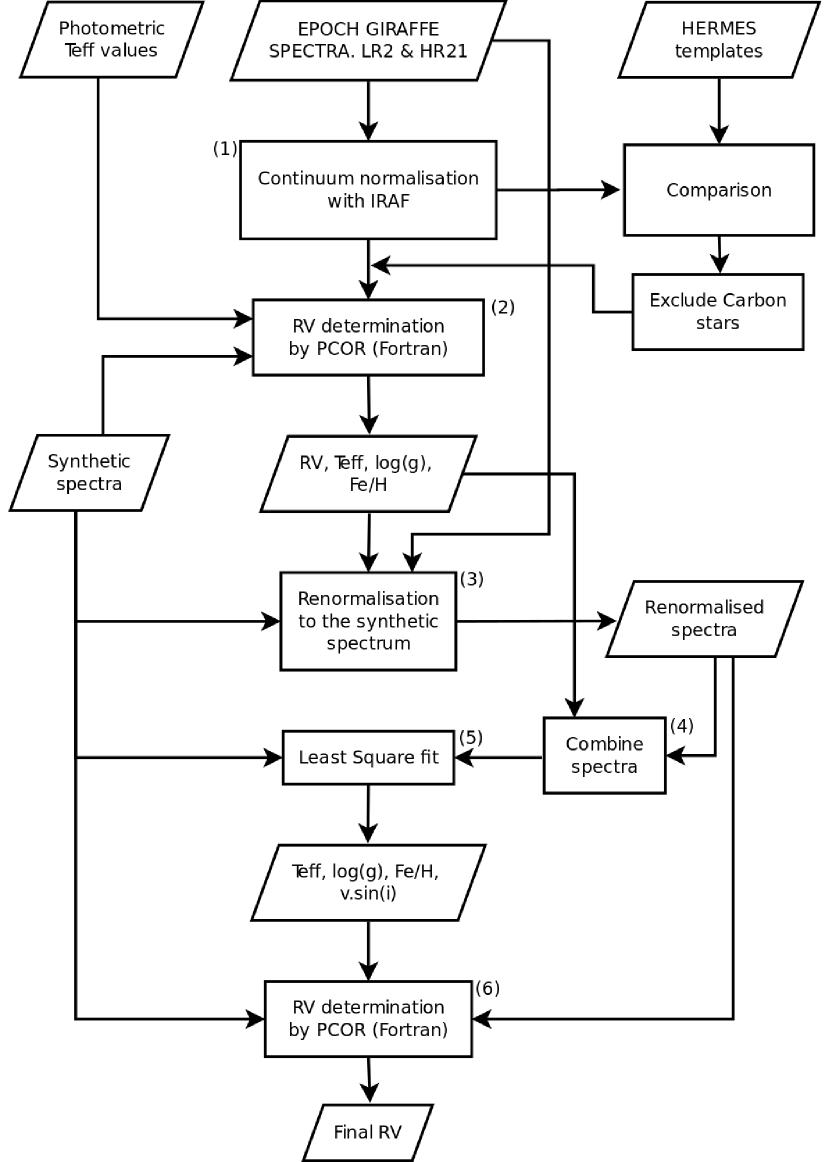
Figure 5: Template optimisation with Pearson Correlation: outline of the procedure described in Sect. 4.1.2

4.1.2 Template optimisation and RV determination

The outline of the procedure which combines various python scripts and one Fortran program is drawn in Fig.5. In a first step (1), the spectra are automatically normalised by means of IRAF’s continuum task. At this point, the carbon stars that we have identified by comparison with the HERMES data (see Sect. 3) are excluded, as no corresponding template spectra are available in our libraries. A first estimate of the radial velocities is done in the next step (2), while the best template is chosen by maximisation of the PCF among a subset of spectra chosen within 500 K of a first estimate of the effective temperature. We obtained this estimate by applying where possible the calibrations of Worthey & Lee (2011) and, to a lesser extent, González Hernández & Bonifacio (2009) to the $BVRI$ photometry (Sect. 2.2) supplemented by $JHK$ magnitudes available in the 2MASS catalogue. When no initial value is available, the choice is made among a predefined list of templates spread over the complete AP space. Accounting for the different metallicity and surface gravity values, it represents 50 to 200 templates to be applied on all HR21, LR2, and UVES spectra available for a given target. Having a first estimate of RV as well as of the astrophysical parameters, all the spectra are renormalised (3) using the currently available optimised template. This part of the work is performed by fitting a polynomial of second (HR21) and third (LR2) order through the ratio of the observed and synthetic spectra, then by applying this normalisation function to the observations. For the GIRAFFE data, the choice of the polynomial was done by performing the operation manually on the spectra of a few targets with different spectral types and observed through the 3 periods (P84, P86, and P88), while UVES data were considered individually. All the normalised observed spectra (including those with $\mathrm{SNR}<5$) of a given star in a given setup were then corrected for the RV shift derived from step (2) and co-added (we computed an average weighted by their SNR) (4). In step (5), all available synthetic spectra are compared to the combined spectrum in order to select the final best template (in terms of sum of square differences) as well as the additional potential line broadening term (we will refer to it as $\varv\sin{i}$, but it may also include other broadening mechanisms difficult to disentangle from each other such as macro-turbulence). The last RV measurement is performed by applying the final best template to the newly normalised observed spectra (6). The stars’ EID, their astrophysical parameters ($T_{\mathrm{eff}}$, $\log g$, $[\mathrm{Fe/H}]$, and [$\mathrm{\alpha/Fe}$]) and, where needed, the $\varv\sin{i}$  of the final templates are provided in Table 4.1.2.

longtablerrrrrr Stellar parameters ($T_{\mathrm{eff}}$, $\log g$, $[\mathrm{Fe/H}]$, [$\mathrm{\alpha/Fe}$], and – where needed – the $\varv\sin{i}$) of the final best template used with the PCOR procedure (The complete version of the table will be made available at the CDS.)
EID $T_{\mathrm{eff}}$ $\log g$ $[\mathrm{Fe/H}]$ [$\mathrm{\alpha/Fe}$] $\varv\sin{i}$
(K) (dex) (dex) ($\mathrm{km}\,\mathrm{s}^{\mathrm{-1}}$)
continued.
EID $T_{\mathrm{eff}}$ $\log g$ $[\mathrm{Fe/H}]$ [$\mathrm{\alpha/Fe}$] $\varv\sin{i}$
(K) (dex) (dex) ($\mathrm{km}\,\mathrm{s}^{\mathrm{-1}}$)
21404 5500 4.0 $-$0.25 0.1
21498 6500 4.0 0.25 0.0 20
22969 C star
22979 4750 2.0 0.00 0.4

4.2 Linelist cross-correlation with DAOSPEC

DAOSPEC (Stetson & Pancino 2008) is an automated Fortran program to measure equivalent widths of absorption lines in high-quality stellar spectra (roughly, spectra with resolving power $\mathcal{R}$$\gtrsim$10 000 and SNR$\gtrsim$30). It cross-matches line centres found in the spectrum (first by a second-derivative filter, and later refined by Gaussian fits) with a list of laboratory wavelengths provided by the user. DAOSPEC is generally used to measure EWs, but an RV determination based on the cross-correlation is also provided. The quality of the resulting RV is expected to be comparable to other methods, albeit with a slightly larger scatter. This is caused by the fact that only the line centre information is used, compared to cross-correlation methods that use all pixels in a spectrum or in a set of pre-defined regions. In the context of this paper, we also tested DAOSPEC outside its validity regime, i.e., LR2 spectra at low SNR ($\mathcal{R}$ $<$20 000 and SNR generally below 30). As a result, we saw that not only the determined RVs tend to be more scattered than those obtained with template or mask cross-correlation spectra, but there was a systematic offset, that increases slightly as SNR decreases, $T_{\mathrm{eff}}$  decreases, or $[\mathrm{Fe/H}]$  increases. This confirms that DAOSPEC can only be used within the validity limits stated in Stetson & Pancino (2008) in terms of SNR and spectral resolution. Within its validity limits, however, DAOSPEC produces results that are well comparable to those obtained with cross-correlation methods, and can thus be used to produce scientifically useful RV measurements as a direct by-product of any EW-based abundance analysis.

To test DAOSPEC on the spectra presented in Section 2.1, we prepared a raw linelist with the help of a dozen synthetic spectra in a range of expected effective temperatures ($4000$ to $6000\mathrm{K}$), surface gravities ($0.8$ to $4$ dex), and metallicities (from $0.0$ to $-1.5\leavevmode\nobreak\ \mathrm{dex}$). The synthetic spectra were created with the Kurucz atmospheric models and synthe code (Castelli & Kurucz 2003; Kurucz 2005; Sbordone et al. 2004) and with the GALA (Mucciarelli et al. 2013) visual inspector sline. Clean, unblended lines were selected and their laboratory wavelengths were taken from VALD3 (Ryabchikova et al. 2011). We ran DAOSPEC through the DOOp self-configuration wrapper (Cantat-Gaudin et al. 2014) leaving the RV totally free, and then created a cleaned linelist by selecting only lines that were measured in at least three spectra. A second run of DOOp/DAOSPEC with the cleaned linelist produced the final observed RVs.

In a few cases DAOSPEC crashed, and there were spectra with discrepant parameters. All these spectra were visually inspected and — when appropriate — re-run imposing a starting RV within $10$ $\mathrm{km}\,\mathrm{s}^{\mathrm{-1}}$around the values obtained for other spectra of the same star. The vast majority of the problematic cases happened with LR2 spectra, as expected. While we treated the UVES RED–L and RED–U spectra separately ($\overline{\Delta\mathrm{RV}_{\mathrm{UL}}}=0.22\pm 0.77$ $\mathrm{km}\,\mathrm{s}^{\mathrm{-1}}$, for 201 spectra), in the following sections and for method to method comparison purposes, both determinations corrected for the shift of the telluric lines were averaged to provide one single value per epoch.

4.3 Mask cross-correlation with iSpec

iSpec is an integrated spectroscopic software framework with the necessary functions for the measurement of radial velocities, the determination of atmospheric parameters and individual chemical abundances (Blanco-Cuaresma et al. 2014). iSpec includes several observed and synthetic masks and templates for different spectral types that can be used to derive radial velocities by cross-correlation. However, very few of them cover the full wavelength range of our target spectra. For this work we chose to cross-correlate the LR2, HR21 and UVES spectra (UVES RED–L and RED–U spectra treated independently), with a mask built on the atlas of the Sun published by Hinkle et al. (2000) and which ranges from $373$ nm to $930$ nm. The cross-correlation of a target spectrum with that mask provides a velocity profile, the peak of which is fitted with a second order polynomial. iSpec also provides the RV error and FWHM of the correlation function fitted by a Gaussian. Due to the large number of spectra we are dealing with in this study, it is not possible to check each cross-correlation visually. We thus developed an automatic processing pipeline which can identify the most uncertain determinations of RV.

For each target spectrum, two coarse estimates of RV were first obtained over a large interval, from $-$500 to $+$500 $\mathrm{km}\,\mathrm{s}^{\mathrm{-1}}$, with a step of 5 $\mathrm{km}\,\mathrm{s}^{\mathrm{-1}}$ and with a step of 1 $\mathrm{km}\,\mathrm{s}^{\mathrm{-1}}$. If the two resulting values differ significantly, this is an indication of a poor cross-correlation. After several tests, we found that it was the most efficient way to detect unreliable determinations which can be due to fast rotation, bad SNR, binarity, or spectral mismatch. Such bad determinations were rejected. They represent $\sim$1% of the LR2 and HR21 determinations, but 8% and 17% of the UVES spectra covering the shorter and longer wavelength part, respectively. For well behaving cross-correlations a more precise RV was determined by using a step of 0.5 $\mathrm{km}\,\mathrm{s}^{\mathrm{-1}}$ over an interval of $\pm$50 $\mathrm{km}\,\mathrm{s}^{\mathrm{-1}}$ around the first velocity estimation. When both determinations are available, the UVES RED–L and RED–U RV values ($\overline{\Delta\mathrm{RV}_{\mathrm{UL}}}=0.16\pm 0.46$ $\mathrm{km}\,\mathrm{s}^{\mathrm{-1}}$, for 187 spectra) were averaged to provide one single measurement per epoch.

5 Results

5.1 Comparison between the different methods

The radial velocities derived by the three methods were compared with one another, and the variation of their relative deviations, $\Delta\mathrm{RV}$, is plotted as a function of $T_{\mathrm{eff}}$  (obtained in Sect. 4.1.2) in Figs. 6 and 7 for the HR21 and LR2, and UVES data, respectively. The comparison was made for all spectra with SNR$\geq$5. Because in the HR21 and LR2 wavelength ranges hot stars have too few available spectral lines, often broadened due to higher rotation, and blended to strong hydrogen lines, we decided not to use the iSpec (Sect. 4.3) and DAOSPEC (Sect. 4.2) methods above 7000 K and therefore limited our comparison to the cooler stars which represent 99% of our sample.

Figure 6: Method to method comparisons for the HR21 (left panel) and LR2 (right panel) data: RV differences are plotted as a function of the effective temperature (dark blue points). The blue boxes extend from the lower to the upper quartile, while the whiskers cover the range of values without outliers from which the median was computed (red horizontal bar).

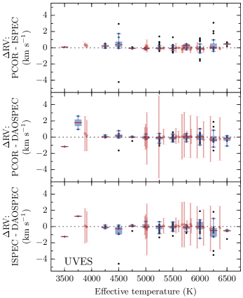
Figure 7: Method to method comparisons for the UVES data: RV differences are plotted against the effective temperature. The blue points are the measurements obtained for the SEP targets, while the red disks represent the Gaia RV standards. The blue boxes extend from the lower to the upper quartile, while the whiskers cover the range of values without outliers from which the median was computed (red horizontal bar). The $T_{\mathrm{eff}}$ is taken from the results of the template optimisation with PCOR (Sect. 4.1.2).

Table 3: Method to method biases derived per $T_{\mathrm{eff}}$  range

$T_{\mathrm{eff}}$ range	$\overline{\Delta\mathrm{RV}}$	$\sigma$	$\overline{\Delta\mathrm{RV}}$/$\sigma$
(K)	($\mathrm{km}\,\mathrm{s}^{\mathrm{-1}}$)	($\mathrm{km}\,\mathrm{s}^{\mathrm{-1}}$)
LR2
PCOR vs iSpec
3500 - 5500	$+$0.020	0.134	0.150
5500 - 8000	$-$0.060	0.239	0.251
PCOR vs DAOSPEC
3500 - 5500	$-$2.108	0.103	20.452
5500 - 8000	$-$2.316	0.169	13.691
iSpec vs DAOSPEC
3500 - 8000	$-$2.208	0.154	14.374
HR21
PCOR vs iSpec
$<$ 3500	$-$0.410	0.370	1.108
3500 - 5500	$-$0.040	0.032	1.268
5500 - 8000	$+$0.100	0.148	0.674
PCOR vs DAOSPEC
$<$ 3500	$+$0.431	0.288	1.494
3500 - 5500	$-$0.077	0.034	2.289
5500 - 8000	$+$0.298	0.167	1.780
iSpec vs DAOSPEC
3500 - 8000	$-$0.032	0.039	0.812
UVES
PCOR vs iSpec
3250 - 8000	$-$0.050	0.034	1.492
PCOR vs DAOSPEC
3250 - 8000	$-$0.056	0.034	1.650
iSpec vs DAOSPEC
3250 - 8000	$-$0.040	0.054	0.737

The method to method offset or bias, $\Delta\mathrm{RV}$, was estimated from the median of the differences. As various libraries of synthetic spectra (BT-Setl, Coelho et al. 2005, MARCS) were used with the PCOR procedure to cover the full $T_{\mathrm{eff}}$  range (Sect. 4.1), the offset of the method relatively to the other ones was derived, where possible, for each grid separately.

The determinations are listed in Table 3 with their $T_{\mathrm{eff}}$  range, median bias ($\overline{\Delta\mathrm{RV}}$), corresponding error ($\sigma$), and the ratio between the bias and the error. The latter value being used to assess the bias significance using a two-tailed test (eq. 20, David et al. 2014). At the 1% significance level, it implies for what follows that an offset between two collections of measurements will be judged significant if the corresponding $\overline{\Delta\mathrm{RV}}$/$\sigma$ ¿ 2.57.

In Fig.6, the method to method differences show a larger scatter in the LR2 wavelength domain than in the HR21 with a slight trend toward 4000 K, its absolute value tending to increase with decreasing temperature. This should be related to the nature of the methods and to their behaviour toward line blending (stronger in cooler stars) and resolving power (lower in LR2). The dispersion of the RV differences between methods varies from 0.34 $\mathrm{km}\,\mathrm{s}^{\mathrm{-1}}$ for UVES data to 2.24 $\mathrm{km}\,\mathrm{s}^{\mathrm{-1}}$ in the LR2 results, while the bias is lower than 0.5 $\mathrm{km}\,\mathrm{s}^{\mathrm{-1}}$ except in LR2 where it peaks at 2.32 $\mathrm{km}\,\mathrm{s}^{\mathrm{-1}}$ in absolute value. At the 1% significance level, if the bias-to-error ratio given in Table 3 is larger than 2.57, the measurements are definitely biased. We will therefore consider that all three methods are providing consistent results, except in LR2 where, according to its limits of applicability (see Sect. 4.2), measurements obtained by DAOSPEC show a systematic bias relative to iSpec and PCOR. LR2 is indeed a region with a weaker signal and a lot of heavily blended spectral atomic and molecular lines that may bias their individual localisation. As a consequence, the LR2 results obtained by DAOSPEC were not considered in what follows.

longtablerlrrrrrrrrrr Epoch radial velocity determinations. Observations with SNR $<$ 5 are shown in italics for information purposes only, but are not further taken into account in the discussion. The table provides: the stars’ EID, the considered observing mode, the SNR, the heliocentric Julian date, the final de-trended multi-epoch barycentric RV determinations for each method as well as their weighted mean and corresponding error bar ($\sigma_{\rm RV}$). (The complete version of the table will be made available at the CDS.)
ISPEC XCOR.D DAOSPEC W.Mean
EID Reg. SNR HJD RV $\sigma_{\rm RV}$ RV $\sigma_{\rm RV}$ RV $\sigma_{\rm RV}$ RV $\sigma_{\rm RV}$
($\mathrm{km}\,\mathrm{s}^{\mathrm{-1}}$) ($\mathrm{km}\,\mathrm{s}^{\mathrm{-1}}$) ($\mathrm{km}\,\mathrm{s}^{\mathrm{-1}}$) ($\mathrm{km}\,\mathrm{s}^{\mathrm{-1}}$) ($\mathrm{km}\,\mathrm{s}^{\mathrm{-1}}$) ($\mathrm{km}\,\mathrm{s}^{\mathrm{-1}}$) ($\mathrm{km}\,\mathrm{s}^{\mathrm{-1}}$) ($\mathrm{km}\,\mathrm{s}^{\mathrm{-1}}$)
continued.
ISPEC XCOR.D DAOSPEC W.Mean
EID Reg. SNR HJD RV $\sigma_{\rm RV}$ RV $\sigma_{\rm RV}$ RV $\sigma_{\rm RV}$ RV $\sigma_{\rm RV}$
($\mathrm{km}\,\mathrm{s}^{\mathrm{-1}}$) ($\mathrm{km}\,\mathrm{s}^{\mathrm{-1}}$) ($\mathrm{km}\,\mathrm{s}^{\mathrm{-1}}$) ($\mathrm{km}\,\mathrm{s}^{\mathrm{-1}}$) ($\mathrm{km}\,\mathrm{s}^{\mathrm{-1}}$) ($\mathrm{km}\,\mathrm{s}^{\mathrm{-1}}$) ($\mathrm{km}\,\mathrm{s}^{\mathrm{-1}}$) ($\mathrm{km}\,\mathrm{s}^{\mathrm{-1}}$)
21404 HR21 1 55271.64688 297.13 0.23 16.24 3.52 -15.92 3.69 0.16 2.55
21404 HR21 4 55285.57863 -24.10 1.32 6.59 1.26 7.43 1.15 7.01 0.85
21404 HR21 11 55519.85760 8.04 0.74 6.73 0.50 8.00 1.14 8.02 0.68
21404 HR21 19 55521.75806 6.96 0.77 5.28 0.36 5.37 0.54 5.32 0.32
21404 LR2 3 55521.83296 -4.38 1.00 9.39 1.63 – – 2.50 0.96
21404 LR2 2 55522.78352 2.89 0.67 10.26 1.78 – – 6.58 0.95
21404 LR2 9 55592.59354 4.46 2.60 4.55 0.40 – – 4.50 1.31
21498 HR21 1 55271.64688 299.45 0.23 561.31 8.77 216.03 12.49 257.74 6.25
21498 HR21 2 55285.57863 194.84 0.31 494.15 7.15 -20.88 1.65 222.70 2.45
21498 HR21 10 55519.85760 300.37 0.40 296.64 0.81 249.11 1.32 298.51 0.45

The combined RV determinations of 380 stars observed in both the HR21 and LR2 domains and with combined errors less than 2 $\mathrm{km}\,\mathrm{s}^{\mathrm{-1}}$ were used to estimate the bias between the 2 GIRAFFE setups as plotted in Fig. 8. To construct this graph all significant method measurements available for one star in one of the 2 domains were combined into a median. The datasets are significantly biased by 1.42 $\mathrm{km}\,\mathrm{s}^{\mathrm{-1}}$, with a dispersion of 1.12 $\mathrm{km}\,\mathrm{s}^{\mathrm{-1}}$. Because the number of stars that each were observed in LR2 and UVES is too small (i.e., 14) and that these spectra have a lower SNR, we first placed the LR2 measurements in the HR21 RV-scale. Then, for those stars having a combined RV error smaller than 1 $\mathrm{km}\,\mathrm{s}^{\mathrm{-1}}$, the comparison between GIRAFFE and UVES data is shown in Fig. 9 and provides a median offset of 0.35 $\mathrm{km}\,\mathrm{s}^{\mathrm{-1}}$ for a semi-interquantile dispersion of 0.40 $\mathrm{km}\,\mathrm{s}^{\mathrm{-1}}$. This offset is of the same order and sign as the median telluric-line shift ($\rm{0.49}\pm\rm{0.74}$ $\mathrm{km}\,\mathrm{s}^{\mathrm{-1}}$) we found in Sect. 2.1.1, and of the same order as those found in the Gaia ESO survey (e.g, lower panel of Fig. 5 in Sacco et al. 2014) with other GIRAFFE observing modes and using a different reduction pipeline. It can therefore be considered as not directly related to the data calibration issues. In both cases (HR21 vs LR2 and GIRAFFE vs UVES), no significant global temperature dependence was found. We subtracted the bias from each individual GIRAFFE measurement. Then, after having filtered out the outliers by applying the Chauvenet criterion in 3 successive iterations, we have combined the two or three RV measurements by computing their weighted mean and corresponding uncertainties.

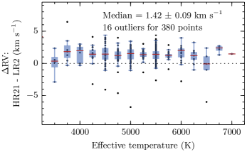
Figure 8: Determination of the RV bias between HR21 and LR2: Differences between the star per star RV median derived in HR21 and LR2 are plotted against the effective temperature (dark blue points). The blue boxes extend from the lower to the upper quartile, while the whiskers cover the range of values without outliers from which the median was computed (red horizontal bar). The median of the differences, its standard deviation, and the number of outliers according to Chauvenet’s criterion are provided.

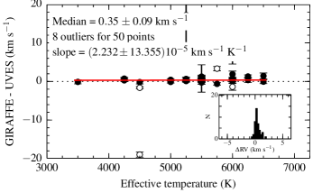
Figure 9: Determination of the RV offset between combined GIRAFFE and UVES measurements: RV differences are plotted as a function of the effective temperature. Open disks are outliers. The median of the differences and the corresponding standard deviation are provided, as well as the slope of the best fit drawn (red line) through the points. Height outliers were filtered out by applying Chauvenet’s criterion.

The results are stored in Table 5.1, with the stars’ EID, the considered observing mode, the SNR, the heliocentric Julian date, the final de-trended multi-epoch barycentric RV determinations for each method, as well as their weighted mean and corresponding error bar ($\sigma_{\rm RV}$).

5.2 Comparison with the catalogue of radial velocity standard stars for Gaia

We have corrected all the measurements for the internal biases and brought our radial velocities on the same scale, but we still need to check how the results compare to the framework defined by the RV standard stars compiled by the IAU Commission 30. Therefore, in the ESO archive, we retrieved 76 UVES spectra of 20 targets in common with the catalogue of RV standard stars for Gaia (Soubiran et al. 2013). We adopted the astrophysical parameters proposed in the PASTEL database (Soubiran et al. 2010) and applied to these data the same procedures and methods as above (see RV results in Fig. 7, red disks). The comparison of these results with the measurements found in the catalogue is shown in Fig. 10. UVES radial velocities appear to be systematically overestimated by $\rm{0.22}$ $\mathrm{km}\,\mathrm{s}^{\mathrm{-1}}$ for an inter-quantile dispersion of 0.12 $\mathrm{km}\,\mathrm{s}^{\mathrm{-1}}$, which is a known offset for UVES as it is of the same order and sign as the median deviation ($8\pm 17$ mÅ  redwards of 5200 Å) obtained by Hanuschik (2003) between the sky line positions in the UVES and Keck atlases. Although it should be accounted for when compared to other catalogues, we prefer to let the user decide to apply the correction and to not include it in our tabulated values.

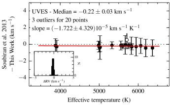
Figure 10: Gaia RV standard stars: comparison between UVES RV measurements (this work) and those found in the Soubiran et al. (2013) catalogue. The median of the differences and the corresponding standard deviation are provided, as well as the slope of the best line drawn (red line) through the points. The histogram distribution of the deviations are provided in the Figure inset. Outliers were filtered out by applying Chauvenet’s criterion.

5.3 Multi-epoch analysis

Most targets were observed at least twice a night, then later during the other periods. Fig. 11 shows the distribution of the time span between 2 spectra of the same star. Our widest time coverage (808 days) was obtained for target EID 80185.

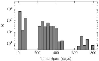
Figure 11: Distribution of the time span between 2 observations of a same target.

For a given star, we combined all individual epoch measurements from all methods into one single value. In order to take into account the RV scatter — which may not be due only to random errors — in the final error bar estimate, we assumed that the errors of each measurement follows a normal distribution. Then we applied a Monte-Carlo scheme with 1000 realisations per determination, and we computed for each star the median and corresponding semi-interquantile dispersion.

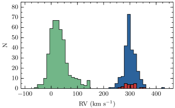
Figure 12: Median RV distribution: Stars with RVs lower or equal than 200 $\mathrm{km}\,\mathrm{s}^{\mathrm{-1}}$ are counted in the green bins, other targets fall in the blue ones. C and S stars are identified by red hatched bins.

The distribution of the combined RVs is shown in Fig. 12. It features two main stellar populations belonging to the LMC and to the Milky Way (MW), with radial velocities larger or smaller than 200 $\mathrm{km}\,\mathrm{s}^{\mathrm{-1}}$, respectively. The results are stored in Table 5.3, which provides the star’s EID, the median RV ($\overline{RV}$), its error bar ($\sigma_{\mathrm{\overline{RV}}}$), the total number of individual measurements used to compute the median (n), the number of epochs (N), and the time span of the observations. For the stars found to have variable photometry by OGLE, Table 5.3 also gives the corresponding period of photometric variation and the OGLE variability flags (Soszyński et al. 2012) in the last columns.

A significant part of the stars in our sample show small to large amplitude radial velocity scatter. To identify the most constant ones, we estimated, method per method, the consistency of the epoch RV measurements ($RV_{i}$ and corresponding error $\sigma_{i}$) and of their weighted mean, $\left\langle{RV}\right\rangle$, we computed the scatter as follows

$$\chi^{2}=\sum_{i}\left(\left\langle{RV}\right\rangle-RV_{i}\right)^{2}/\sigma_{i}^{2}$$ (1)

as well as the associated probability, $P(\chi^{2})$, that the deviations are within the known error boundaries. From the method by method analysis of these deviations, we deduce that 34 out of the 489 stars with more than 2 measurements have $\mathrm{P(}\chi^{\mathrm{2}}\mathrm{)}<10^{\mathrm{-6}}$ and show significant RV variations whatever the method used. Those stars are noted ”VAR” in Col. (7) of Table 5.3. Additionally, 44 targets ranked ”VAR” by at least 2 methods or with $\mathrm{P(}\chi^{\mathrm{2}}\mathrm{)}<0.00135$ for all 3 methods are labelled ”VAR?”. Conversely, stars having $P(\chi^{2})\geq 0.00135$, more than 2 measurements spread over a time span larger than 180 days, with $\sigma_{\rm\overline{RV}}<$ 1 $\mathrm{km}\,\mathrm{s}^{\mathrm{-1}}$, and which therefore does not show any significant RV scatter in the results of all 3 methods are noted ”RV-REF” in Table 5.3 (represents 145 stars). If one of the criteria above, on time span or on $\sigma_{\rm\overline{RV}}$, is not fulfilled, then the target received the ”RV-REF?” label (represents 125 stars). For the remaining 141 objects (of the 489), nothing conclusive can be inferred.

longtablerrrrrrrrr Median radial velocities, LMC membership, and variability status: The table provides the star’s EID, the median RV ($\overline{RV}$), its error bar ($\sigma_{\mathrm{\overline{RV}}}$), the total number of individual measurements used to compute the median (n), the number of epochs (N), and the time span of the observations. When useful, we provide in col. (7) a few remarks in the form of labels: LMC (bona fide LMC member), LMC? (possible LMC member), VAR (RV variable), VAR? (prossible RV variable), RV-REF (target with constant RV over the time span), RV-REF? (possibly constant in RV), Ca ii K em. (shows emission in the Ca ii K line), Ca ii T em. (shows emission in the Ca ii triplet), and H i em. (shows emission in the Paschen lines). For the stars found to have variable photometry by OGLE, we further give in the last columns the corresponding period of photometric variation and the OGLE variability flags (Soszyński et al. 2012). (The complete version of the table will be made available at the CDS.)
OGLE
EID $\overline{RV}$ $\sigma_{\mathrm{\overline{RV}}}$ $n$ $N$ Time Span Remark(s) Period VAR flag
($\mathrm{km}\,\mathrm{s}^{\mathrm{-1}}$) ($\mathrm{km}\,\mathrm{s}^{\mathrm{-1}}$) (days) (days)
continued.
OGLE
EID $\overline{RV}$ $\sigma_{\mathrm{\overline{RV}}}$ $n$ $N$ Time Span Remark(s) Period VAR flag
($\mathrm{km}\,\mathrm{s}^{\mathrm{-1}}$) ($\mathrm{km}\,\mathrm{s}^{\mathrm{-1}}$) (days) (days)
21404 6.16 0.46 8 3 72.74 RV-REF?
21498 297.53 0.78 12 5 72.74 VAR
22969 308.19 0.17 5 5 320.95 LMC, C Star 51.17 LPV/OSARG
23916 72.48 1.25 2 1 0.00

6 Discussion

6.1 Astrophysical parameters

The astrophysical parameters of the best matching synthetic spectrum are by-products of the template optimisation scheme adopted with the PCOR program (Sect. 4.1.2). To have an estimate of their consistency level, we compared the effective temperatures obtained with this procedure to those found in the literature of the best corresponding matching HERMES spectrum (Sect. 3). The differences between the former and latter determinations are plotted in Fig. 13 in function of the $V-R$ colour. Distinction is made between stars with RV smaller and larger than 200 $\mathrm{km}\,\mathrm{s}^{\mathrm{-1}}$ (see Sect. 6.3). If we except a few outliers, all points fall within 1000 K, with a median value and dispersion of $30\pm 335\mathrm{K}$ (black histogram in inset of Fig. 13). Although the distribution looks symmetric, deviations follow a trend with $V-R$: stars with $\mathrm{RV}\geq 200$ $\mathrm{km}\,\mathrm{s}^{\mathrm{-1}}$  showing on average an offset of $-120\pm 260\mathrm{K}$, the other ones have differences of the order of $140\pm 340\mathrm{K}$. Such behaviour may have various origins. It can be due to the non-completeness of the libraries (e.g., in terms of $[\mathrm{Fe/H}]$), to the model assumptions (e.g., 1D atmosphere models for red giants) or to the accuracy of the atomic data used to compute the spectra. Anyhow, we generally have a fair agreement between the observed and final synthetic spectra, and — as will be shown hereafter — we have a good consistency between the resulting APs ($T_{\mathrm{eff}}$, $\log g$, and $[\mathrm{Fe/H}]$) and the different stellar populations to be expected in the MW and LMC. A lower estimate of the template mismatch effects and of the parameter errors on the RV determinations can be deduced from Fig. 1 in David et al. (2014). In our temperature range and assuming deviations of 500 K, this would lead to biases of the order of 200 $\mathrm{m}\,\mathrm{s}^{\mathrm{-1}}$, which is of the same order as our smallest RV error bars.

Figure 13: Effective temperature deviations versus $V-R$: Differences are between the effective temperature of the best HERMES template and the one derived during synthetic template optimisation. Stars with RV ¡ 200 $\mathrm{km}\,\mathrm{s}^{\mathrm{-1}}$ are shown in green, while the other ones are in blue. The histogram of the deviations is given in the Figure inset, with the same colour coding and with the complete distribution shown in black.

6.2 Variability

It is reasonable to suspect that part of the detected RV variability (Sect. 5.3) is due to stellar multiplicity, to pulsations or to any other astrophysical phenomenon at the origin of RV jitter. Unfortunately, we currently do not have a sufficient number of observations to model the variations and to derive non degenerate solutions. A few targets, however, show clear spectroscopic evidence for a companion. Seven have confirmed RV variability, while we lack sufficient data for the other two (EID 50823 and EID 98406). In Table 5.3, we labelled ”SB2” or ”SB2?” these targets with composite spectra.

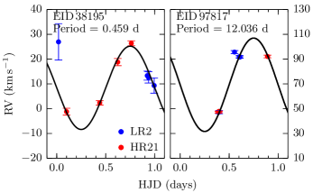
Figure 14: Phase diagrams of the eclipsing EID 38195 (left panel) and SB1 EID 97817 (right panel) binaries

Among the 5 eclipsing binaries identified by OGLE, 3 are also SB2. It is the case of EID 84084, for which we plot in Fig. 15 the HR21 spectroscopic variability. EID 38195 is detected VAR, but its variations cannot be directly phased with the photometric period of 0.45 d. We therefore submitted its RVs to a multi-step RV-curve fitting procedure developed by Damerdji et al. (2012) and found a close solution at P = 0.459 d (Fig. 14, left panel).We only have two LR2 epoch measurements for EID 72521, which therefore was not classified VAR by our procedure even though the difference between the 2 RVs is significant (i.e., $P(\chi^{2})<10^{\mathrm{-6}}$).

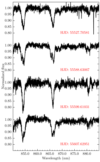
Figure 15: Spectroscopic variations of the eclipsing SB2 EID 84084.

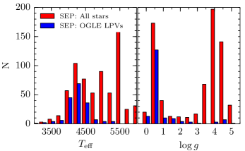
Figure 16: Distribution of $T_{\mathrm{eff}}$  and $\log g$  among SEP and LPV stars

Four stars have ellipsoidal variations in the OGLE data. Two (EID 30581 is VAR and EID 96413 is VAR?) are spectroscopically variable. EID 107847 does not show any significant RV variation over a period of time of 385 days in the 7 UVES spectra, while the OGLE period is 302 days. EID 92169 was observed 9 times over 347.92 days. It exhibits a larger RV scatter ($\sim 3$ $\mathrm{km}\,\mathrm{s}^{\mathrm{-1}}$), but this is not sufficient for it to be detected as variable by applying our various criteria.

Among the identified VAR and VAR? stars, 17 show photometric long period variability in the OGLE catalogue as would be expected from evolved cool stars. If one excepts EID 97817, all these stars have a $\log g$ $<2.5$ and have RVs compatible with the LMC. More generally, as shown in Fig. 16, the majority of stars flagged ”LPV” by OGLE have $T_{\mathrm{eff}}$  and $\log g$  consistent with those found for red giants. Because EID 97817 exhibits quite a high amplitude RV scatter and astrophysical parameters that do not belong to an evolved cool star, we suspect it to be a SB1 rather than an LPV. As a matter of fact, the orbit fitting procedure of Damerdji et al. (2012) proposes a solution at the exact same OGLE period (Fig. 14, right panel).

EID 50856 is noted by OGLE to be a galactic RR Lyrae, which agrees with its magnitude ($V=16.37$) and with the astrophysical parameters of the nearest synthetic spectrum ($T_{\mathrm{eff}}$ $=6250\mathrm{K}$, $\log g$ $=4.0$, and $[\mathrm{Fe/H}]$ $=-1.5$). Two of the RV methods found it variable in RV. The rather high median RV (i.e., $420.43\pm 1.53$ $\mathrm{km}\,\mathrm{s}^{\mathrm{-1}}$) and its low $[\mathrm{Fe/H}]$  suggests that it is a halo population II star.

6.3 LMC membership

The one-square-degree SEP field covers a small part of the LMC. Therefore a significant number of stars in our sample are LMC members, with radial velocities different from those found on average in the MW. Indeed we find a double-peaked RV distribution (Fig. 12) with one top at $\sim 24$ $\mathrm{km}\,\mathrm{s}^{\mathrm{-1}}$ and another at $\sim 298$ $\mathrm{km}\,\mathrm{s}^{\mathrm{-1}}$. As shown by the $\log g$  and $[\mathrm{Fe/H}]$  estimates (Fig. 17), stars with RV $\geq$ 200 $\mathrm{km}\,\mathrm{s}^{\mathrm{-1}}$ further tend to be $[\mathrm{Fe/H}]$  depleted (e.g., Thevenin & Jasniewicz 1992) and have a surface gravity lower than 2.5 as we expect for the brightest members of the LMC. In our sample, 203 targets with radial velocities larger than 200 $\mathrm{km}\,\mathrm{s}^{\mathrm{-1}}$, $\log g$ $<2.5$, and metallicities lower than in the Sun can therefore be regarded as bona fide LMC members. In addition, 51 more stars have RVs consistent with the LMC but higher metallicities or higher $\log g$. Among the 178 targets with OGLE LPV variability flagged, 169 belong to these LMC or candidate LMC stars, which do confirm their red giant status. Both categories are respectively labelled ”LMC” and ”LMC?” in Table 5.3 and are highlighted in Fig. 1. LMC stars appear to be randomly distributed over the SEP field, and follow no obvious structure.

Figure 17: $[\mathrm{Fe/H}]$  and $\log g$  distributions of the SEP targets

6.4 Targets of particular interest

Nine G and K-type SEP stars show emission-like features, sometimes variable, in the near-IR Calcium triplet and/or in the blue Ca ii K line (see Fig. 18). These stars, which generally have $\log g$$\geq 4$ (exceptions are EID 77381 and EID 102310) are tagged ”Ca ii K and T em.” or ”Ca ii K em.” in Table 5.3 and probably are chromospherically active. Among these, EID 88013 shows periodic photometric variability due to spots. In addition, 1 B-type supergiant, EID 68904, exhibits emission in its hydrogen Paschen lines (”H i em.” in Table 5.3).

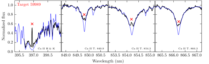
Figure 18: Comparison between the best fitted template (dashed blue curve) and the observed LR2 and HR21 data of EID 59989 (solid curve). Signs of chromospherical activity are detected in the core of the calcium lines (red crosses).

The comparison of the GIRAFFE spectra with HERMES data (Sect. 3), led us to find a few stars with features only seen in evolved objects and which we identified as carbon (18 targets) and S stars (6 targets). All these objects have RVs typical of those found in the LMC. The C stars further already have an entry in the carbon star catalogue of Kontizas et al. (2001). As we do not have any mask nor synthetic spectrum adapted to C stars, we derived their radial velocity using high SNR data of VY UMa.

Due to the random fibre allocation, we could identify one galaxy (Fig. 19) already mentioned in the 2M++ galaxy redshift catalogue (Lavaux & Hudson 2011). By fitting the corresponding averaged LR2 and HR21 data with synthetic spectra, we estimated a redshift of 0.026.

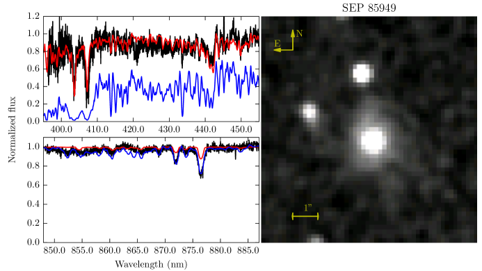
Figure 19: The observed spectra (black curve) of the Galaxy EID 85949 is compared to 2 theoretical stellar spectra computed with the same $T_{\mathrm{eff}}$  and $\log g$  (4000 K and 1.00, respectively), but having a different metallicity. The blue line spectrum has a Solar-like metallicity, while the red one is depleted by $-$2.5 dex. Both spectra are shifted by $\mathrm{RV}=7810$ $\mathrm{km}\,\mathrm{s}^{\mathrm{-1}}$ ($z=0.026$) to match the observations.

7 Conclusions

Among the 747 targets selected at random in the 1-square-degree field centred around the South Ecliptic Pole and observed with FLAMES, 725 had spectra with $\mathrm{SNR}\geq 5$. By visually inspecting these and by performing a systematic comparison with HERMES observations, we identified one galaxy, 18 C stars, and 6 new S stars, while the use of various libraries of synthetic spectra provided us with a first stellar classification. As a main result, we measured the radial velocities on all the FLAMES (UVES and GIRAFFE) data by applying 3 different methods in order to assess their zero-point and precision. From the RV, $[\mathrm{Fe/H}]$, and $\log g$  distributions we have extracted 203 objects that are bona fide LMC members, and 51 that have RVs and $[\mathrm{Fe/H}]$  or $\log g$  values compatible with those we expect for the LMC in the considered magnitude ranges. Multi-epoch observations enabled us to identify 78 RV variable stars as well as to highlight those targets with the most stable radial velocity (145 stars). Seven confirmed SB2s — among which 3 are eclipsing — and 2 candidate SB2 stars have composite spectra.

In Gaia commissioning, the satellite had several periods of Ecliptic Pole Scanning Law (EPSL), during which the satellite repeatedly scanned the North and South Ecliptic Poles (i.e. each pole was observed twice) every 6 hours. These periods allowed Gaia’s Radial Velocity Spectrometer (RVS, Katz et al. 2004; Cropper & Katz 2011) to collect a large number of observations of the GIRAFFE and UVES stars presented in this article. These were used to validate the RVS ground-based processing pipeline (Katz et al. 2011) and to make a first appraisal of its radial velocity performance for the faint-magnitude stars (Cropper et al. 2014; Seabroke et al. 2015). Now that the routine mission is on-going, the SEP GIRAFFE-UVES sample is part of the nominal RVS ground-based processing pipeline. It is used to monitor and assess the convergence of the RVS performance in the faint star regime.

Tables found in pages 1 to 12 are available in the electronic edition of the journal at http://www.aanda.org as well as at the CDS in electronic format.