Differentially-Private Counting of Users’ Spatial Regions

Abstract

Mining of spatial data is an enabling technology for mobile services, Internet-connected cars, and the Internet of Things. But the very distinctiveness of spatial data that drives utility, can cost user privacy. Past work has focused upon points and trajectories for differentially-private release. In this work, we continue the tradition of privacy-preserving spatial analytics, focusing not on point or path data, but on planar spatial regions. Such data represents the area of a user’s most frequent visitation—such as “around home and nearby shops”. Specifically we consider the differentially-private release of data structures that support range queries for counting users’ spatial regions. Counting planar regions leads to unique challenges not faced in existing work. A user’s spatial region that straddles multiple data structure cells can lead to duplicate counting at query time. We provably avoid this pitfall by leveraging the Euler characteristic for the first time with differential privacy. To address the increased sensitivity of range queries to spatial region data, we calibrate privacy-preserving noise using bounded user region size and a constrained inference that uses robust least absolute deviations. Our novel constrained inference reduces noise and promotes covertness by (privately) imposing consistency. We provide a full end-to-end theoretical analysis of both differential privacy and high-probability utility for our approach using concentration bounds. A comprehensive experimental study on several real-world datasets establishes practical validity.

1 Introduction

The ubiquity, quality and usability of location-based services supports the ready availability of user tracking. Location data sharing is used across a wide range of applications such as traffic monitoring, facility location planning, recommendation systems and contextual advertising. The distinctiveness of location data, however, has led to calls for location privacy Beresford03 ; Gruteser2004 : the ability to track users in aggregate without breaching individual privacy. There exists a spectrum of approaches to address location privacy Chow2011 ; Chow2011Trajectory ; Ghinita2013 ; Krumm07 with significant attention having been paid to range queries on point location or trajectory data: for example, providing statistics of how many mobile users are presently on an arterial road.

Typical private spatial analytics supports point locations or sequences of points (see Figure 1a). Points and trajectories, however, do not best-represent user location in all applications. In facility-services planning, a planner may wish to locate a new department store in a location that overlaps with users’ regions of frequent visitation. While hotel-booking sites collect area-level information about customers’ preferred destinations. Such problems motivate our focus on counting private planar bodies (see Figure 1b). Given a collection of privacy-sensitive planar bodies representing regions of frequent location, we wish to support counting range queries while preserving individual privacy. Figure 1b illustrates this task, on a map of metropolitan Melbourne with planar bodies representing regions of individual users’ frequent visitation. Third parties may wish to submit any number of queries requesting the number of users’ areas falling in a specified query region, e.g., for urban transport planning or retail analytics.

A leading approach for responding to range queries in spatial data analytics is aggregation Papadias2001 ; Papadias2002 ; Tao2002 ; Tao2004 ; Lopez2005 ; Braz2007 ; Marketos2008 ; LeonardiORRSAA14 ; Timko2009 . Initial interest in aggregation was due to computational efficiency considerations and early data structures promote these properties. More recently aggregation has been used as a qualitative approach to privacy, as it is a natural choice for privacy-preserving data release Chawla2005 .

In the setting of planar bodies, conventional grid-partitioned histograms cannot provide accurate results due to the duplicate counting problem as a planar body may span more than one histogram cell simultaneously. This is a problem unique to counting planar bodies. To address this challenge, we instead leverage the Euler characteristic trudeau1993introduction where face, edge and vertex counts are stored separately. Such Euler histograms Beigel1998 permit exact counting of convex planar bodies SunAA02 ; Sun2002 ; Sun2006 (cf. Section 3.1 and Figure 2).

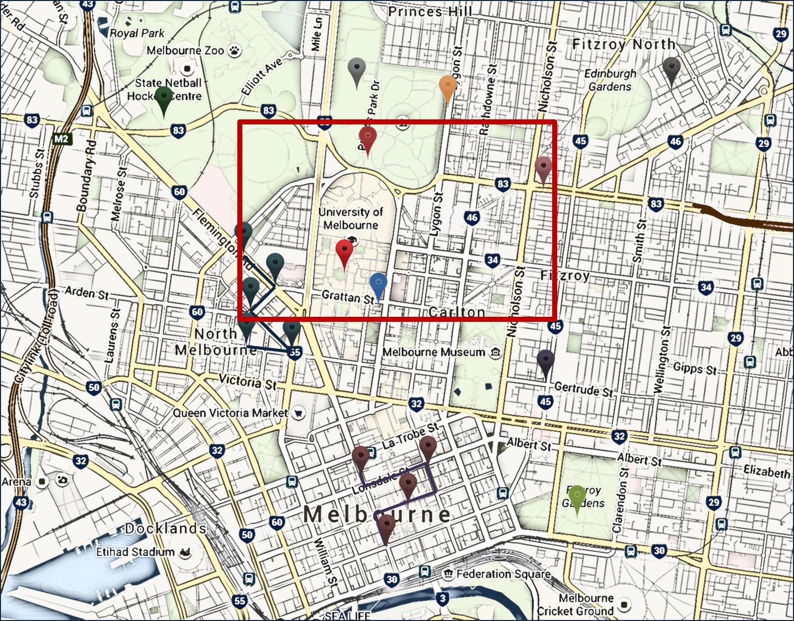
(a) Point locations or sequence of points (trajectories) as typical spatial representatives of a user.

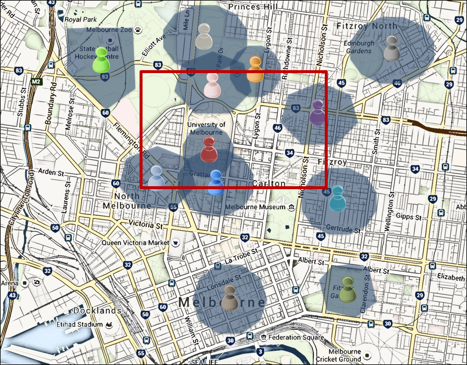
(b) Users’ regions of frequent visitation; each user’s spatial data is represented by a single planar body.

Figure 1: Example users’ point locations (path) or spatial regions on a map of Melbourne. Bolded rectangle depicts an example range query to count the number of users.

The recently emerged strong guarantee of differential privacy Cynthia2006 ; Dwork08 has attracted a number of researchers in location privacy. Typically work studies aggregation of point and trajectory data InanKGB10 ; ChenFDS12 ; Cormode12PSD ; QardajiYL13 ; HeCMPS15 , often via histogram-like data structures—regular or hierarchical—for controlling the level of perturbation required for privacy.

Our goal in this paper is to address the accurate counting of planar bodies, while providing the strong guarantee of differential privacy. While Euler histograms provide an excellent starting point in terms of utility, computational efficiency and aggregation-based qualitative privacy, a service provider may be directed by users to provide strong semantic privacy. Differential privacy guarantees that an attacker with significant prior knowledge and computational resources cannot determine presence or absence of a user in a set of planar bodies.

Differential privacy requires randomization. The challenge in combining the ideas of Euler histograms and differential privacy is that the data structure’s large number of counts require randomised perturbation. As a result, the total noise added could be prohibitively high. Compared to point data in which at most one cell is impacted per record, here an object could span more than one cell, impacting many counts. Naive solutions would therefore significantly degrade utility. Moreover when sampled independently, perturbations can destroy the consistency of query responses over the resulting structure Barak2007 .

The first stage of our approach is to perturb counts of a Euler histogram by applying noise controlled via sensitivity to a natural bound on planar body size. Then, to re-instate consistency and improve utility with no cost to privacy, we apply constrained inference that seeks to minimally update counts to satisfy consistency constraints. These constraints reflect relationships between data structure counts that must exist, but may be violated by perturbation. Under these constraints we apply least absolute deviations (LAD), which is more robust to outliers than ordinal regression—used previously for constrained inference in differential privacy. By enforcing consistency, we also “average out” previously-added noise, thereby improving utility in certain cases. Finally, we round counts so that query responses are integral. This final stage, combined with consistency, yields responses that preserve a covertness property such that third-party observers cannot determine that privacy-preserving perturbation has taken place.

Two privacy models have been studied for releasing datasets or their statistics: the interactive and non-interactive models Cynthia2006 . In the non-interactive setting, the database is sanitized and then released while the interactive model considers mechanisms that respond to queries by releasing approximate query responses. The main limitation with this latter approach is the limited number of queries permitted throughout the mechanism’s lifetime. Interactive mechanisms (e.g., Euler histograms CASE2015 ) can provide inconsistent results also. Our focus is on the non-interactive privacy setting, wherein our mechanisms release privacy-preserving data structures to third parties, with no limitation on the number of subsequent query responses permitted.

Contributions.

We deliver several main contributions:

• For the first time, we address the differentially-private counting of planar bodies (spatial region objects) in the non-interactive setting;

• We propose differentially-private mechanisms that leverage the Euler characteristic (via the Euler histogram data structure) to address the duplicate counting problem;

• We formulate novel constrained inference to reduce noise and introduce consistency based on the robust method of least absolute deviations; combined with rounding, this guarantees a covertness property;

• We contribute an end-to-end theoretical analysis of both high-probability utility and differential privacy; and

• We conduct a comprehensive experimental study on real-world datasets, which confirms the suitability of our approach to private range queries on spatial bodies.

2 Related Work

A series of effective privacy attacks on location data Gruteser2004 ; Krumm07 ; Ghinita2013 has launched a significant amount of activity around privacy-preserving techniques for spatial analytics Chow2011 ; Ghinita2013 ; Krumm09 .

Aggregation under range queries has emerged as a fundamental primitive in spatial and spatio-temporal analytics Papadias2001 ; Tao2004 ; Lopez2005 ; Braz2007 ; LeonardiORRSAA14 . Originally motivated by statistical and computational efficiency, aggregation is now also used for qualitative privacy.

A key challenge in aggregation is the distinct counting Papadias2001 ; Tao2004 ; Lopez2005 ; Braz2007 ; LeonardiORRSAA14 or multiple-counting problem SunAA02 ; Sun2006 . In contrast to point objects, a spatial body can span more than one cell in a partitioned space, inhibiting the ability of regular histograms to form accurate counts. Euler histograms Beigel1998 are designed to address this problem for convex bodies SunAA02 ; Sun2006 , by appealing to Euler’s formula from graph theory trudeau1993introduction . A variation of Euler histogram has been studied for trajectory data to address aggregate queries on moving objects Xie2007 . In that work, Euler histograms were used in a distributed setting (motivating a distributed Euler histogram), to tackle the duplicate (distinct) entry problem rather than duplicate (distinct) counting. The Euler-histogram tree Xie2014 has been studied as a tree-based data structure for counting vehicle trajectories using the approach first developed in CASE2015 to address the distinct counting problem for reducing storage requirements.

There is a line of work CASE2015 , in which the CASE histogram has been proposed as a privacy-preserving approach for trajectory data analytics, where only count data is utilised in a partitioned space applying the Euler characteristic to address duplicate counting. The authors in CASE2015 discuss the interactive setting for differentially-private Euler histogram release, which has a prohibitive limitation of the number of queries being linear in the number of bodies. Our work has no such limitation (see Dwork08 ).

Differential privacy Cynthia2006 ; Dwork08 has now become a preferred approach to data sanitisation as it provides a strong semantic guarantee with minimal assumptions placed on the adversary’s knowledge or capabilities. Differential privacy has been studied for location privacy Ghinita2013 . One existing approach is to obfuscate the user’s location by perturbing their real geographic coordinates. The concept of geo-indistinguishability has been defined AndresBCP13 ; PrimaultMLB14 as a notion of differential privacy in location-based services. Due to its popularity, differential privacy has been applied to many algorithms and across many domains, such as specialized versions of spatial data indexing structures designed with differential privacy for the purpose of private record matching InanKGB10 ; in spatial crowdsourcing to help volunteer workers’ locations remain private ToGS14 ; in machine learning, releasing differentially-private learned models of SVM classifiers Rubinstein12 ; in geo-social networks for location recommendation ZhangGC14 ; and for modelling human mobility from real-world cellular network data Mir13 .

Within the scope of aggregation, studies in the area of point privacy have also proposed sanitization algorithms for generating differentially-private histograms and releasing aggregate statistics. Many studies have explored differential privacy of point sets AcsCC12 ; InanKGB10 ; Cormode12PSD ; ChenFDS12 ; WangZM13 ; FanXS13 ; HeCMPS15 ; QardajiYL13 ; LiHay14 . They have studied regular grid partitioning data structures and hierarchical structures. This work for the first time addresses the problem of differentially-private counting of planar bodies.

Table 1, demonstrates various techniques for privacy preserving spatial analytics using aggregates comparing privacy model, data type and approach.

Table 1: Taxonomy on private spatial data analytics using aggregates with examples of related work.

Privacy Model	Data Type	Approach
Spatial Aggregation	Trajectory	Probabilistic counting using sketches—approximation method (Tao et al. Tao2004 ) Distributed Euler Histograms (DEHs) addressing distinct-entry counting problem (Xie et al. Xie2007 ), Count-based approach similar to Xie2007 (Leonardi et al. LeonardiORRSAA14 ) CASE histograms, addressing distinct-object counting problem (duplicate counting) CASE2015
Differential Privacy	Point	Quad-tree, KD-tree (Cormode et al. Cormode12PSD ), Uniform and Adaptive Grid (Qardaji et al. QardajiYL13 )
Differential Privacy	Trajectory	Prefix tree (Chen et al. ChenFDS12 ), DPT, using hierarchical reference systems (He et al. HeCMPS15 ), CASE Histograms CASE2015
Differential Privacy	Spatial Region (Planar Body)	Differentially private Euler histograms (this work)

3 Preliminaries

One natural but qualitative approach to privacy preservation is spatial aggregation. We will leverage a data structure that permits spatial aggregation for body counts.

3.1 Euler Histograms

Given a grid partitioned space, an Euler histogram data structure allocates buckets not only for grid cells, but also for grid cell edges and vertices. We formally define the data structure as below.

Definition 1

Consider an arbitrary partition of a subset of $\mathbb{R}^{2}$ into convex cells. Define $\mathcal{F}$, $\mathcal{E}$, $\mathcal{V}$ to be index sets over the partition’s faces, edges (face intersections), and vertices (edge intersections). Let $\mathbf{P}$ be a vector with components, the faces, edges and vertices, indexed by $\mathcal{F}\cup\mathcal{E}\cup\mathcal{V}$ (i.e., each $P_{i}\subset\mathbb{R}^{2}$ represents a face/edge/vertex area of the Euclidean plane); and let vector $\mathbf{H}$ of non-negative integers be indexed by $\mathcal{F}\cup\mathcal{E}\cup\mathcal{V}$ as well (representing counts per face/edge/vertex). Then we call the data structure $(\mathbf{P},\mathbf{H},\mathcal{F},\mathcal{E},\mathcal{V})$ an Euler histogram.

Originally, Euler histograms were designed as a grid partitioning data structure, but they are valid for other convex partitions as well. For example, valid Euler histograms could be defined over a Voronoi partition of space induced by a finite set of sensors as the sites of a Voronoi diagram detecting any object in their region Xie2007 ; or a rectangular partition over an urban area CASE2015 such as in Figure 2.

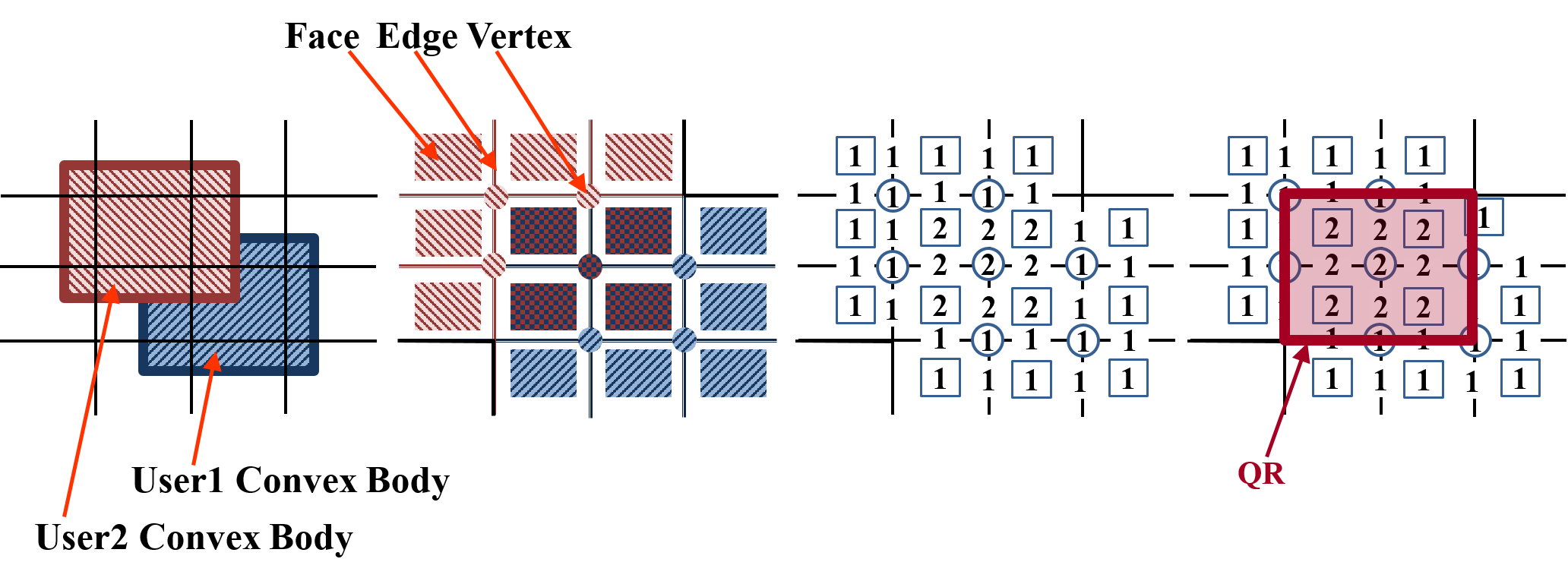
Figure 2: Two convex bodies overlapping a spatial partition and their related counts to corresponding Euler histogram; an example query region (QR) to count the number of objects.

Beigel and Tanin Beigel1998 first introduced to spatial databases, the observation that the Euler characteristic trudeau1993introduction (including its extensions to higher dimensions) directly applies to this data structure. Euler’s characteristic states that the number of convex bodies $N$ overlapping certain query regions can be computed exactly as

$$N=F-E+V\enspace,$$ (1)

where $F,E,V$ are the sum of face, edge, and vertex counts in $\mathbf{H}$ within the given query region (QR in Figure 2). Duplicate counting due to summing face counts is corrected by subtracting edge counts. This in turn can over-compensate, and is corrected by adding vertex counts. This is a special case of the Inclusion-Exclusion Principle of set theory and applied probability. Figure 2 illustrates the impact two planar bodies have on a square-partition Euler histogram. Compared to conventional histograms, with the use of extra counts for grid cell edges and vertices, large objects spanning more than one cell are now distinguishable from several small objects intersecting only one cell. Applying Equation (1) to calculate the number of objects inside the highlighted QR of Figure 2, we arrive at the correct answer of $N=8-8+2=2$.

3.2 Differential Privacy

We consider statistical databases on records—each representing a user’s spatial region. Randomisation is vital for preventing an adversary from inverting a released statistic to reconstruct the original (private) data.

Definition 2

A randomised mechanism $\mathcal{M}(D)$ on database $D$, is a random variable taking values in response set $Range(\mathcal{M})$.

Definition 3

We say that two databases $D$, $D^{\prime}$ are neighbours if they are of equal size and differ on exactly one record—one spatial body representing a user in the context of this paper.

Definition 4

A randomised mechanism $\mathcal{M}$, is said to preserve $\epsilon$-differential privacy for $\epsilon>0$, if for all neighbouring databases $D$, $D^{\prime}$, which differ in exactly one record, and measurable $C\subseteq Range(\mathcal{M})$:

$$\mathrm{Pr}(\mathcal{M}(D)\in C) \leq \exp(\epsilon)\cdot\mathrm{Pr}(M(D^{\prime})\in C)\enspace.$$

Definition 4 implies that an algorithm is differentially private if a change, addition or deletion of a record, does not significantly affect the output distribution. Differential privacy has become a de facto standard for privacy of input data to statistical databases due to it being a semantic guarantee Cynthia2006 .

Remark 1

The threat model of differential privacy involves an incredibly powerful adversary with full knowledge of mechanism $\mathcal{M}$, all but one record of true latent database $D$, the ability to sample from $\mathcal{M}(D)$, and unlimited computational power. Using these capabilities, an optimal attack for reconstructing $D$ is to sample $m_{1},\ldots,m_{k}\stackrel{{\scriptstyle iid}}{{\sim}}\mathcal{M}(D)$. From this sample the attacker can form a histogram that is an empirical estimate $\hat{}\mathcal{M}(D)$ of the true response distribution $\mathcal{M}(D)$. Knowing that the true $D$ is neighbouring to the database $D^{\prime}$ known by the attacker, they may simulate (using their unbounded computational resources) each and every response distribution $\mathcal{M}(D^{\prime\prime})$ for neighbouring $D^{\prime\prime},D^{\prime}$ and then attempt to match these against $\hat{M}(D)$. Differential privacy states exactly that each of the simulated candidate response distributions are exceedingly similar (multiplicatively pointwise close), and so for sufficiently small $\epsilon$ (relative to sample size $k$ which is limited to linear in size of $D$) it is impossible for the attacker to distinguish the true $\mathcal{M}(D)$ by comparison with $\hat{}\mathcal{M}(D)$.

Lemma 1 (Post-Processing Immunity Cynthia2006 )

For any randomised algorithm $\mathcal{M}:\mathcal{X}\rightarrow\mathcal{R}$ and any (possibly randomised) function $f:\mathcal{R}\rightarrow\mathcal{R^{\prime}}$, if $\mathcal{M}$ is $\epsilon$-differentially private then $f\circ\mathcal{M}$ is also $\epsilon$-differentially private.

Lemma 1 implies that differential privacy is immune to post-processing. This is also referred as Transformation Invariance, as one of the privacy axioms Kifer2010 , indicating that post-processing privatised data maintains privacy.

4 Problem Statement

The focus of this paper is to respond to range queries over spatial datasets consisting of a spatial region per user.

Problem 1

Given a set of planar bodies, our goal is to batch process them to produce a data structure that can respond to an unlimited number of range queries within some fixed, bounded area: given a query region QR, we are to respond with an approximate count of bodies overlapping that region.

For example, a range query covering the entire area in Figure 1b might elicit a response of (exact count of) 12.

4.1 Evaluation Metrics

We consider four properties of mechanisms, as competing metrics for evaluating solutions to Problem 1.

1. Utility: We measure utility by the absolute error of query responses relative to the true count of bodies intersecting a given query region.

2. Privacy: Mechanisms should achieve non-interactive differential privacy, at some level $\epsilon$, in their release of a data structure on sensitive spatial data.

3. Consistency: If responses to all possible queries agree with some fixed set of bodies then we say that the mechanism is consistent. Such a set of bodies need not coincide with the original input bodies.

4. Covertness: If a consistent counting mechanism’s query responses are non-negative integer-valued, then we also call it covert.

Utility and privacy are in direct tension, for establishing privacy typically involves reducing the influence of data on responses. However for fixed levels of privacy, for example, we can ask what levels of utility are possible for available solutions to Problem 1.

If privacy-preserving perturbations are made independently across a data structure, it is unsurprising that overlapping queries will not necessarily result in consistent responses. This may be undesirable for some applications that utilise multiple, overlapping queries e.g., urban planning. We consider specific, public consistency constraints which relate to the data structure adopted. As such, the level of consistency can be benchmarked according to the number of consistency violations suffered. Unlike privacy, consistency is not necessarily at odds with utility: indeed we will demonstrate how imposing consistency can actually improve utility. Intuitively, if privacy-preservation involves injecting independent, random perturbations to a data structure, then consistency corresponds to a public smoothness assumption that can be used to ‘cancel out’ the deleterious effect of perturbation. Consistency may also be applied when a measure of ‘stealth’ is desired for a counting mechanism.

4.2 Assumptions

The theoretical guarantees developed in this paper leverage four assumptions (cf. Figure 3). Each is relatively weak, being well motivated and satisfied in most practical settings.

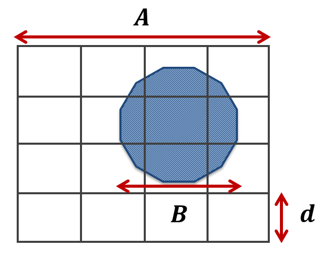
Figure 3: A convex body with bounded diameter, on a spatial partition.

1. We assume that the space partition’s cells are all convex.

2. We assume that query regions are convex unions of our space partition’s cells.

3. We assume that all planar bodies are convex.

4. We assume that all planar bodies are of some bounded $L_{2}$ diameter $B>0$.

A sufficient condition for correctness of Equation (1), is that all objects are convex planar bodies. However, convexity is not necessary. In general, objects being disconnected leads to inaccurate counts. Note that connected objects can become disconnected e.g., a concave object not contained by a query region CASE2015 . Our first three assumptions are sufficient for guaranteeing correctness (perfect utility) for Euler histograms. Relaxing these assumptions may come at the cost of utility. For example convex query regions that are not unions of cells can exactly count the number of bodies in the (enlarged) union of cells intersecting the QR. And general query regions will still result in excellent utility. Two important partition geometries satisfy these conditions: rectangular and Voronoi partitions.

The fourth assumption controls the $L_{1}$-Lipschitz smoothness of Euler histogram counts with respect to input bodies. This parameter—also known as the global sensitivity (cf. Definition 5)—calibrates the scale of noise added for differential privacy. We consider a motivating example to be regions of frequent visitation. These are necessarily bounded. With $B$ sufficiently large, no restriction is made on valid bodies.

Without loss of generality we assume partitions are square of side length $A>0$, divided into $n$ rows and $n$ columns, yielding square cells of side length $d=A/n$ (cf. Figure 3).

5 Algorithms and Analysis

Our approach consists of four complementary algorithms:

• Euler (Eu): Euler histogram construction from a set of convex planar bodies;

• DiffPriv (DP): Calibrated perturbation of histogram counts to achieve $\epsilon$-differential privacy. To improve utility, negative counts are truncated at zero;

• LinProg (LP): Constrained inference for consistency;

• Round (R): Rounding counts for covertness.

We detail each mechanism, followed by its theoretical analysis. Figure 4 depicts an example run of each algorithm in turn. As shown, Figure 4a illustrates two users’ spatial regions, our running example in Figure 2, as input raw data for the first Algorithm 1 (cf. Section 5.1).

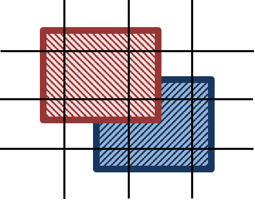
(a) Two users’ planar bodies.

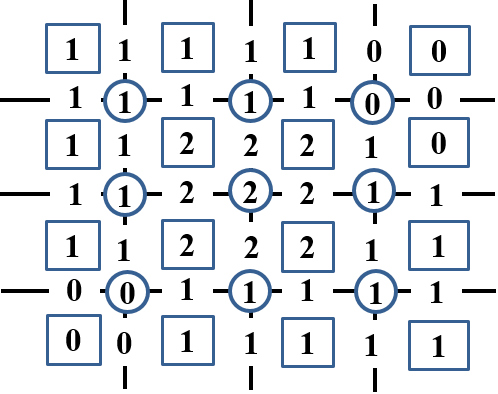
(b) Euler histogram construction.

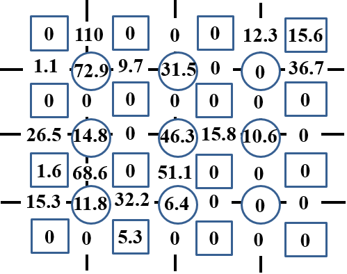
(c) Perturbing the counts (DP).

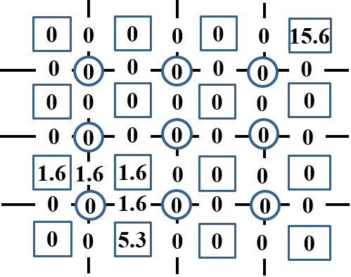
(d) Linear programming (LP).

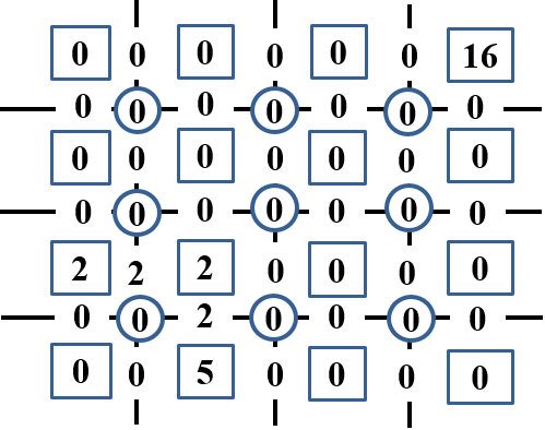
(e) Rounding the counts (R).

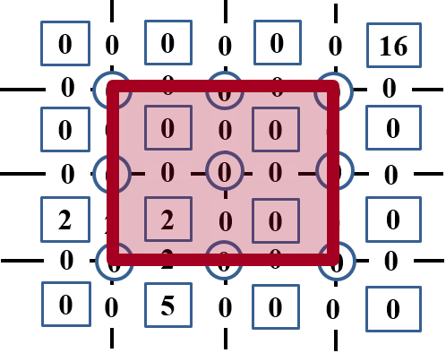
(f) Example range query response.

Figure 4: An example of the mechanisms’ outputs; numbers from a real run.

5.1 Algorithm: Euler

Algorithm 1 creates a data structure (Euler histograms cf. Section 3.1) to represent aggregated counts of a given set of convex planar bodies $\mathcal{X}$. The algorithm simply increments counts for any face, edge, vertex that intersects a body. As shown in Figure 4b, processing a convex body determines what counts need to be incremented.

Input : Set of planar bodies $\mathcal{X}$; partition $(\mathbf{P},\mathcal{F},\mathcal{E},\mathcal{V})$

Output : Euler histogram $(\mathbf{H},\mathbf{P},\mathcal{F},\mathcal{E},\mathcal{V})$

1 for $i\in\mathcal{F}\cup\mathcal{E}\cup\mathcal{V}$ do

2       $H_{i}\longleftarrow 0$

3for $x\in\mathcal{X}$ do

4       for $i\in\mathcal{F}\cup\mathcal{E}\cup\mathcal{V}$ do

5             if  $x\cap P_{i}\neq\emptyset$ then

6                   $H_{i}\longleftarrow H_{i}+1$

7            

8      

9

10

Algorithm 1 Euler (Eu): Euler Histogram Construction

Privacy.

Euler is qualitatively private via aggregation, but it does not achieve any differential privacy by virtue of being deterministic.

Utility.

Assumptions A1–A3 guarantee the preconditions of the following, direct results of Equation (1).

Corollary 1

If input bodies, partition cells, and query region are convex, and the query region is a union of cells, then Euler’s responses to the range query via Equation (1) are accurate.

Corollary 2

Euler is consistent (P3) and covert (P4).

Computational Complexity.

As our partition has $n$ rows and columns, Euler’s time and space complexities are efficient at $O(\lvert\mathcal{X}\rvert n^{2})$ and $O(n^{2})$ respectively.

5.2 Algorithm: DiffPriv

Euler achieves a number of our target properties but not differential privacy. We now introduce differential privacy to our approach by perturbing Euler histogram counts. In Algorithm 2, we add carefully-crafted random noise based on the sensitivity of the histogram to input bodies. We truncate any resulting negative counts to zero, improving utility at no cost to privacy (cf. Lemma 1). Figure 4c depicts the result of this phase for a real example. For interested readers, the computed global sensitivity (GS) (cf. Definition 5 and Lemma 2) of this example is $25$, where $\lceil B/d\rceil=2$, and the allocated privacy budget, $\epsilon$, is $1$.

Privacy.

The key step to establishing the differential privacy of DiffPriv, is to calculate Lipschitz smoothness for Euler—the scale of noise to be added to reduce sensitivity. This represents how sensitive Euler is to input bodies, and so how much noise should be added to reduce this sensitivity for privacy.

Definition 5

Let $f$ be a deterministic, real-vector-valued function of a database. The $L_{1}$-global sensitivity (GS) of $f$ is given by $\Delta f=\max\limits_{D,D^{\prime}}\lVert f(D)-f(D^{\prime})\rVert_{1}$, taken over all neighbouring pairs of databases.

The $L_{1}$-global sensitivity is a property of function $f$, independent of input database. For Euler histograms, the GS measures the effect on the histogram count vector, due to changing an input planar body related to a user’s spatial region.

Lemma 2

The $L_{1}$-global sensitivity of Euler is $4.5\Big{(}\left\lceil\frac{B}{d}\right\rceil+1\Big{)}\left\lceil\frac{B}{d}\right\rceil$, where $d>0$ is the cell side length, and $B>0$ is an $L_{2}$ bound on planar body diameter.

Proof

By Assumption 4 (cf. Figure 3), the number of cells that could intersect with a body is at most $\left\lceil\frac{B}{d}\right\rceil+1$ in one direction. Therefore the total number of cells that could intersect a body is

$$n^{2} \leq \left(\left\lceil\frac{B}{d}\right\rceil+1\right)^{2}\enspace.$$

From this the number of faces, edges and vertices of partition $\mathbf{P}$ intersecting with a body can be upper-bounded as

#Faces $$= n^{2}\leq\left(\left\lceil\frac{B}{d}\right\rceil+1\right)^{2}\enspace;$$

#Edges $$\leq 2n(n-1)\enspace;\enspace\mbox{and}$$

#Vertices $$\leq (n-1)^{2}\enspace.$$

Summing these, we may bound the total number of partition components intersected by the body as

$$4n(n-1)+1$$

$$\leq 4\left(\left\lceil\frac{B}{d}\right\rceil+1\right)\left\lceil\frac{B}{d}\right\rceil+1$$

$$= 4\left(\left\lceil\frac{B}{d}\right\rceil+1\right)\left\lceil\frac{B}{d}\right\rceil+\frac{1}{2}\left\lceil\frac{B}{d}\right\rceil^{2}+\frac{1}{2}\left\lceil\frac{B}{d}\right\rceil$$

$$= 4\left(\left\lceil\frac{B}{d}\right\rceil+1\right)\left\lceil\frac{B}{d}\right\rceil+\frac{1}{2}\left(\left\lceil\frac{B}{d}\right\rceil+1\right)\left\lceil\frac{B}{d}\right\rceil$$

$$\leq 4.5\left(\left\lceil\frac{B}{d}\right\rceil+1\right)\left\lceil\frac{B}{d}\right\rceil\enspace.$$

Since changing a single body in a database can affect impacted histogram cell counts by one, this expression is also a bound on global sensitivity.

DiffPriv applies the Laplace mechanism Cynthia2006 to Euler: it adds to a non-private vector-valued function $f$, i.i.d. Laplace-distributed noise with centre zero and scale $\lambda$ given by $\Delta f/\epsilon$, for desired privacy level $\epsilon>0$. Here, $\lambda=\Delta\mathbf{H}/\epsilon$.

Input : Euler histogram: $(\mathbf{P},\mathbf{H},\mathcal{F},\mathcal{E},\mathcal{V})$; privacy $\epsilon>0$; sensitivity $\Delta\mathbf{H}>0$

Output : Noisy histogram: $(\mathbf{P},\mathbf{H}^{\prime},\mathcal{F},\mathcal{E},\mathcal{V})$

1

2for $i\in\mathcal{F}\cup\mathcal{E}\cup\mathcal{V}$ do

3       $H_{i}^{\prime}\longleftarrow H_{i}+Lap(0;\Delta\mathbf{H}/\epsilon)$

4      if  $H_{i}^{\prime}<0$  then

5             $H_{i}^{\prime}\longleftarrow 0$

6      

7

8

Algorithm 2 DiffPriv (DP): Perturbation by Laplace Noise

Corollary 3

DiffPriv preserves $\epsilon$-differential privacy.

Proof

The result follows by applying the triangle inequality to the odds ratio using the definition of Laplace density, and global sensitivity Cynthia2006 .

Utility.

DiffPriv is neither covert nor consistent, however we can bound its utility.

Theorem 5.1

For confidence level $\delta\in(0,1)$, the counts $\mathbf{H}$ output by Euler and counts $\mathbf{H^{\prime}}$ output by DiffPriv are uniformly close with high probability

$$\Pr\left(\lVert\mathbf{H^{\prime}}-\mathbf{H}\rVert_{\infty}\leq\lambda\log\left(\frac{\lvert\mathcal{F}\rvert+\lvert\mathcal{E}\rvert+\lvert\mathcal{V}\rvert}{\delta}\right)\right) \geq 1-\delta\enspace.$$

Proof

For convenience, we define the combined index set $\mathcal{H}=\mathcal{F}\cup\mathcal{E}\cup\mathcal{V}$, noting that $\lvert\mathcal{H}\rvert=\lvert\mathcal{F}\rvert+\lvert\mathcal{E}\rvert+\lvert\mathcal{V}\rvert$. Recall that by the definition of DiffPriv, we have that

$$\forall i\in\mathcal{H}, H^{\prime}_{i}=H_{i}+Y_{i},\enspace Y_{i}\sim Lap(0;\lambda)\enspace.$$

By the cumulative distribution function of the zero-mean Laplace, it follows that

$$\forall~{}i\in\mathcal{H}, \mathrm{Pr}(\lvert Y_{i}\rvert\geq z)=\exp\left(\frac{-z}{\lambda}\right)\enspace,$$

for any scalar $z>0$. By the union bound it follows that

$$\mathrm{Pr}\left(\bigcup\limits_{i\in\mathcal{H}}\{\lvert Y_{i}\rvert\geq z\}\right) \leq \sum_{i\in\mathcal{H}}\mathrm{Pr}(\lvert Y_{i}\rvert\geq z)$$

$$= \lvert\mathcal{H}\rvert\times\exp\left(\frac{-z}{\lambda}\right)\enspace.$$

Applying De Morgan’s law,

$$\mathrm{Prob}\left(\bigcap\limits_{i\in\mathcal{H}}\{\lvert Y_{i}\rvert<z\}\right) = 1-\mathrm{Prob}\left(\bigcup\limits_{i\in\mathcal{H}}\{\lvert Y_{i}\rvert\geq z\}\right)$$

$$\geq 1-\lvert\mathcal{H}\rvert\times\exp\left(\frac{-z}{\lambda}\right)$$

$$\triangleq 1-\delta\enspace.$$

Solving yields

$$z = \lambda\times\log\left(\frac{\lvert\mathcal{H}\rvert}{\delta}\right)\enspace,$$

so that

$$\mathrm{Prob}\left(\bigcap\limits_{i\in\mathcal{H}}\left\{\lvert Y_{i}\rvert<\lambda\log\left(\frac{\lvert\mathcal{H}\rvert}{\delta}\right)\right\}\right) \geq 1-\delta\enspace.$$

The result follows from $\mathbf{H^{\prime}}-\mathbf{H}=\mathbf{Y},\enspace\mathbf{Y}\sim Lap(\lambda)$ iid.

Computational Complexity.

As our partition has $n$ rows and columns, DiffPriv’s time/space complexities are efficient at $O(n^{2})$.

5.3 Algorithm: Linear Programming

After additive randomised perturbation with DiffPriv, we apply constrained inference to smooth this noise, as detailed below. We begin by defining constrained inference, followed by a set of public consistency constraints.

5.3.1 Constrained Inference: LAD

Constrained inference models the noisy counts output by DiffPriv as noisy observation of latent counts which are themselves related according to a set of constraints. Inference effectively smooths the differentially-private release, potentially improving utility without affecting privacy. Previously ordinary least squares (OLS) has driven constrained inference Cormode12PSD ; HayRMS10 . Here we propose instead to use least absolute deviation (LAD) (also referred to as least absolute residuals, least absolute errors and least absolute value) Dielman2005 . In contrast to OLS, LAD has the benefit of being robust to outliers. LAD is ideal for our setting, since its choice of minimising $L_{1}$ error corresponds to maximising the exponential of the negative $L_{1}$: a Laplace noise model, akin to maximum-likelihood estimation, matching DiffPriv precisely.

Definition 6

Let $\mathbf{H}$ be the Euler histogram counts with a set of defined constraints, $\mathcal{C}$. Given noisy histogram counts, $\mathbf{H^{\prime}}$, constrained LAD inference returns vector $\mathbf{H^{\prime\prime}}$, that satisfies the constraints $\mathcal{C}$ while minimising $\lVert\mathbf{H^{\prime\prime}}-\mathbf{H^{\prime}}\rVert_{1}$.

Proposition 1

Suppose Alice ($\mathcal{A}$) wished to communicate to Bob ($\mathcal{B}$) her parameter vector $\boldsymbol{\theta}\in\Theta$ some Euclidean parameter family known to $\mathcal{B}$, but that her communication of $\boldsymbol{\theta}$ passed through a noisy channel specified by the Laplace mechanism: $\mathcal{B}$ observes $\boldsymbol{\theta}$ with additive i.i.d. zero-mean Laplace with known scale $\lambda>0$. Then LAD corresponds to $\mathcal{B}$ using maximum-likelihood estimation to recover $\boldsymbol{\theta}$.

Proof

In this abstract setting (that applies beyond our mechanisms, to the Laplace mechanism more generally) suppose that $\mathcal{B}$ observes via the channel from $\mathcal{A}$

$$X_{i}\stackrel{{\scriptstyle indep.}}{{\sim}}Lap(\theta_{i},\lambda)\enspace,\enspace i\in\{1,\ldots,m\}\enspace.$$

Then the joint likelihood of the $X_{i}$, known to $\mathcal{B}$, is given by

$$\prod_{i=1}^{m}\frac{1}{2\lambda}\exp\left(-\frac{|x_{i}-\theta_{i}|}{\lambda}\right)=\frac{1}{2^{m}\lambda^{m}}\exp\left(-\frac{\|\mathbf{x}-\boldsymbol{\theta}\|_{1}}{\lambda}\right)\enspace.$$

The MLE of unknown $\boldsymbol{\theta}$ given the observations and known scale $\lambda$ corresponds to the constrained optimisation

$$\hat{\boldsymbol{\theta}}_{MLE} \in \arg\max_{\boldsymbol{\theta}\in\Theta}\ \frac{1}{2^{m}\lambda^{m}}\exp\left(-\frac{\|\mathbf{x}-\boldsymbol{\theta}\|_{1}}{\lambda}\right)$$

$$= \arg\max_{\boldsymbol{\theta}\in\Theta}\ \log\left(\exp\left(-\frac{\|\mathbf{x}-\boldsymbol{\theta}\|_{1}}{\lambda}\right)\right)$$

$$= \arg\max_{\boldsymbol{\theta}\in\Theta}\ -\frac{\|\mathbf{x}-\boldsymbol{\theta}\|_{1}}{\lambda}$$

$$= \arg\min_{\boldsymbol{\theta}\in\Theta}\ \|\mathbf{x}-\boldsymbol{\theta}\|_{1}\enspace.$$

The first equality follows from a strictly monotonic transformation of the objective function, the second follows from cancelling the logarithmic and exponential functions, and the final equality follows from another strictly monotonic transformation. This last formulation corresponds to constrained LAD.

The application of this result to our present setting involves equating the latent parameter vector to the raw histogram $\mathbf{H}$, Laplace-perturbed observations to $\mathbf{H}^{\prime}$, and the parameter family $\Theta$ to constraint set $\mathcal{C}$ (to be discussed below). This connection demonstrates that our use of LAD is principled. Given public prior knowledge of counts, one could incorporate a corresponding (public) prior distribution on the $\theta$ and perform maximum a posteriori (MAP) point-estimation which would in-turn correspond to placing a regularisation term on the LAD objective. We leave such extensions to future work.

Consistency.

We define three constraints C1, C2 and C3 for Euler histograms as follows. Our consistency constraints consider the relationships between face, edge and vertex counts. Every increment to an edge count must correspond to an increment to the counts of both incident faces as well; and similarly for an increment to a vertex count, the corresponding four incident edge counts must be incremented. Finally query regions should respond with non-zero count estimates. These represent the intuition behind our three sets of consistency constraints.

For ease of exposition, we refer to face, edge and vertex components of $\mathbf{H}$ by $F_{i},E_{i},V_{i}$ respectively. The meaning will be apparent from context.

Constraint 1

Every edge count is less than or equal to the minimum value of its two incident faces.

$$E^{\prime\prime}_{i}\leq F^{\prime\prime}_{j}\ \ \forall i\in\mathcal{E},\forall j\in\mathcal{F}_{i};\enspace\mathcal{F}_{i}=\{j\in\mathcal{F}:j\text{ incident to }i\in\mathcal{E}\}$$

Constraint 2

Every vertex count is less than or equal to its four incident edges’ counts.

$$V^{\prime\prime}_{i}\leq E^{\prime\prime}_{j}\ \ \forall i\in\mathcal{V},\forall j\in\mathcal{E}_{i};\enspace\mathcal{E}_{i}=\{j\in\mathcal{E}:j\text{ incident to }i\in\mathcal{V}\}$$

Constraint 3

Every two by two grid partition should have a non-negative count computed by Euler, Equation (1).

$$F^{\prime\prime}_{j}-E^{\prime\prime}_{k}+V^{\prime\prime}_{i}\geq 0 \forall i\in\mathcal{V},\forall j\in\mathcal{F}_{i},\forall k\in\mathcal{E}_{i}$$

$$\mbox{where}\ \ \ \ \ \mathcal{F}_{i} = \{j\in\mathcal{F}:j\text{ incident to }i\in\mathcal{V}\}$$

$$\mathcal{E}_{i} = \{k\in\mathcal{E}:k\text{ incident to }i\in\mathcal{V}\}\enspace.$$

Figure 4d demonstrates the output of LinProg algorithm that smooths the noise and applies consistency constraints.

Algorithm.

We consider two constrained inference programs for enforcing these constraints. Both minimise the change to the histogram counts subject to the constraints. The first, LAD, minimises counts with respect to the $L_{1}$-norm.

$$\min_{\mathbf{H^{\prime\prime}}}\lVert\mathbf{H^{\prime\prime}}-\mathbf{H^{\prime}}\rVert_{1}\ \ \mbox{s.t.}\ \mathbf{H^{\prime\prime}}\geq\mathbf{0}\enspace\ \ \text{Constraints }C_{1},C_{2},C_{3}$$

By introducing a primal variable per histogram cell count, we can transform this to the following linear program

$$\min_{\mathbf{H^{\prime\prime}},\mathbf{h}} \sum_{i=1}^{|\mathcal{H}|}h_{i}$$ (2)

s.t. $$\mathbf{H^{\prime\prime}},\mathbf{h}\geq\mathbf{0}$$

$$H^{\prime}_{i}-H^{\prime\prime}_{i}\leq h_{i}\enspace\forall i\in\mathcal{H}$$

$$H^{\prime\prime}_{i}-H^{\prime}_{i}\leq h_{i}\enspace\forall i\in\mathcal{H}$$

$$\text{Constraints }C_{1},C_{2},C_{3}$$

Alternatively we could adopt the $L_{\infty}$-norm for minimising the change to the histogram cell counts, as in the following program.

$$\min_{\mathbf{H^{\prime\prime}}}\lVert\mathbf{H^{\prime\prime}}-\mathbf{H^{\prime}}\rVert_{\infty}\ \ \ \mbox{s.t.}\ \mathbf{H^{\prime\prime}}\geq\mathbf{0}\ \ \ \text{Constraints }C_{1},C_{2},C_{3}$$

And again we may transform this program to an equivalent LP, this time by introducing only a single new primal variable

$$\min_{\mathbf{H^{\prime\prime}},h} h$$ (3)

s.t. $$\mathbf{H^{\prime\prime}},h\geq\mathbf{0}$$

$$H^{\prime}_{i}-H^{\prime\prime}_{i}\leq h\enspace\forall i\in\mathcal{H}$$

$$H^{\prime\prime}_{i}-H^{\prime}_{i}\leq h\enspace\forall i\in\mathcal{H}$$

$$\text{Constraints }C_{1},C_{2},C_{3}$$

We analyse Program (3), however we recommend that in practice Program (2) be used since it is better able to minimise change to all cell counts (and is derived according to the MLE principle as per Proposition 1), while Program (3) only minimises the maximum error. Algorithm 3 and our experiments reflect this recommendation.

Input : Noisy Histogram: $(\mathbf{P},\mathbf{H^{\prime}},\mathcal{F},\mathcal{E},\mathcal{V})$

Output : Consistent Histogram: $(\mathbf{P},\mathbf{H^{\prime\prime}},\mathcal{F},\mathcal{E},\mathcal{V})$

1

2Solve Program (2).

3

Algorithm 3 LinProg (LP): Linear Programming

Privacy.

Since LinProg depends only on the output of DiffPriv, it preserves the same level of differential privacy (cf. Lemma 1).

Utility.

We can establish high-probability utility bounds on LinProg $(L_{\infty})$ that take a similar form to those proved for DiffPriv, but via different arguments.

Theorem 5.2

For any confidence level $\delta\in(0,1)$, and for histogram counts $\mathbf{H^{\prime}}$ output by DiffPriv and $\mathbf{H^{\prime\prime}}$ minimising Program (3), we have

$$\mathrm{Pr}\left(\lVert\mathbf{H^{\prime}}-\mathbf{H^{\prime\prime}}\rVert_{\infty}\leq\lambda\log\left(\frac{\lvert\mathcal{F}\rvert+\lvert\mathcal{E}\rvert+\lvert\mathcal{V}\rvert}{\delta}\right)\right) \geq 1-\delta\enspace.$$

Proof

We reduce to the bound on DiffPriv, by noting that since LinProg is minimising distance, the distance from $\mathbf{H^{\prime\prime}}$ to $\mathbf{H^{\prime}}$ must be no more than $\mathbf{H}$ to $\mathbf{H^{\prime}}$. In other words

$$\overbrace{\lVert\mathbf{H^{\prime}}-\mathbf{H^{\prime\prime}}\rVert_{\infty}}^{\text{LP}} \leq\overbrace{\lVert\mathbf{H^{\prime}}-\mathbf{H}\rVert_{\infty}}^{\text{Laplace Analysis}}\leq \lambda\log\left(\frac{\lvert\mathcal{F}\rvert+\lvert\mathcal{E}\rvert+\lvert\mathcal{V}\rvert}{\delta}\right)$$

with the final bound holding with probability at least $1-\delta$.

Computational Complexity.

Linear programming interior-point methods—also referred to as barrier algorithms—are polynomial-time, with worst-case complexity of $O(a^{3.5})$ Karmarkar1984 , for $a$, the number of variables. Therefore, for Euler histograms the time complexity is $O(n^{7})$, but in practice it is efficient as demonstrated in our runtime experiments (cf. Section 6.10 for running time).

5.4 Algorithm: Rounding

After running LinProg, we introduce covertness via Round (Algorithm 4). This allows the data curator to hide that the data has been perturbed (see Figure4e). Figure 4f depicts an example range query response to privately count the number of users via Equation (1), $N=F-E+V=2$.

Input : Consistent Histogram: $(\mathbf{P},\mathbf{H^{\prime\prime}},\mathcal{F},\mathcal{E},\mathcal{V})$

Output : Rounded Histogram: $(\mathbf{P},\mathbf{H^{\prime\prime\prime}},\mathcal{F},\mathcal{E},\mathcal{V})$

1

2for $i\in\mathcal{F}\cup\mathcal{E}\cup\mathcal{V}$ do

3       $H^{\prime\prime\prime}_{i}\longleftarrow round(H^{\prime\prime}_{i})$

Algorithm 4 Rounding (R)

Privacy.

Since Round depends only on differentially-private data, it also preserves differential privacy (cf. Lemma 1).

Utility.

The analysis of utility for Round is more straightforward than for DiffPriv and LinProg.

Lemma 3

If $\mathbf{H^{\prime\prime}}$ is the output histogram of LinProg and $\mathbf{H^{\prime\prime\prime}}$ is the result of Round, then $\lVert\mathbf{H^{\prime\prime}}-\mathbf{H^{\prime\prime\prime}}\rVert_{\infty}\leq 0.5$.

Lemma 4

Round is consistent when run after LinProg, and so it is also covert.

Proof

We only need to check the consistency constraints, as to whether Round violates any. This cannot happen, since the smaller side of a constraint inequality rounding up must coincide with the larger side rounding up. Similarly the larger side rounding down must coincide with the smaller side doing the same. Therefore, consistency is invariant to rounding.

Computational Complexity.

Similar to DiffPriv since our partition has $n$ rows and columns, Round’s time and space complexities are efficient at $O(n^{2})$.

5.5 Full Theoretical Analysis

We are now able to combine the individual utility analyses of the four stages of our approach, into an overall high-probability bound on utility.

Corollary 4

For confidence level $\delta\in(0,1)$, and histogram counts $\mathbf{H}$, $\mathbf{H^{\prime\prime\prime}}$ output by Euler and Round respectively we have that

$$\lVert\mathbf{H}-\mathbf{H^{\prime\prime\prime}}\rVert_{\infty} \leq \frac{9\big{(}\left\lceil\frac{B}{d}\right\rceil+1\big{)}\left\lceil\frac{B}{d}\right\rceil}{\epsilon}\log\left(\frac{\frac{4A^{2}}{d^{2}}-\frac{4A}{d}+1}{\delta}\right)+0.5$$

holds with probability at least $1-\delta$.

Proof

By Theorems 5.1, 5.2, Lemma 3, triangle inequality

$$\lVert\mathbf{H}-\mathbf{H^{\prime\prime\prime}}\rVert_{\infty} \leq \lVert\mathbf{H}-\mathbf{H^{\prime}}\rVert_{\infty}+\lVert\mathbf{H^{\prime}}-\mathbf{H^{\prime\prime}}\rVert_{\infty}+\lVert\mathbf{H^{\prime\prime}}-\mathbf{H^{\prime\prime\prime}}\rVert_{\infty}$$

$$\leq 2\times\lambda\log\left(\frac{\lvert\mathcal{F}\rvert+\lvert\mathcal{E}\rvert+\lvert\mathcal{V}\rvert}{\delta}\right)+0.5\enspace$$

with high probability , where $\lambda=4.5\left(\left\lceil\frac{B}{d}\right\rceil+1\right)\left\lceil\frac{B}{d}\right\rceil/\epsilon$. Continuing

$$2\times\lambda\log\left(\frac{\lvert\mathcal{F}\rvert+\lvert\mathcal{E}\rvert+\lvert\mathcal{V}\rvert}{\delta}\right)+0.5$$

$$\leq \frac{2\big{[}4\left(\left\lceil\frac{B}{d}\right\rceil+1\right)\left\lceil\frac{B}{d}\right\rceil+1\big{]}}{\epsilon}\log\left(\frac{\lvert\mathcal{F}\rvert+\lvert\mathcal{E}\rvert+\lvert\mathcal{V}\rvert}{\delta}\right)+0.5$$

$$\leq \frac{9\left(\left\lceil\frac{B}{d}\right\rceil+1\right)\left\lceil\frac{B}{d}\right\rceil}{\epsilon}\log\left(\frac{\frac{4A^{2}}{d^{2}}-\frac{4A}{d}+1}{\delta}\right)+0.5\enspace.$$

We have used the following counts, where $n$ is the number of rows/columns in the grid-partitioned area of volume $A^{2}$:

$$\lvert\mathcal{F}\rvert = n\times n=n^{2}=\frac{A^{2}}{d^{2}}\enspace;$$

$$\lvert\mathcal{E}\rvert \leq 2n\times(n-1)=2(n^{2}-n)=2(\lvert\mathcal{F}\rvert-\sqrt{\lvert\mathcal{F}\rvert})\enspace;$$

$$\lvert\mathcal{V}\rvert \leq (n-1)^{2}=n^{2}-2n+1=\lvert\mathcal{F}\rvert-2\sqrt{\lvert\mathcal{F}\rvert}+1\enspace;$$

$$\lvert\mathcal{F}\rvert+\lvert\mathcal{E}\rvert+\lvert\mathcal{V}\rvert \leq \lvert\mathcal{F}\rvert+2(\lvert\mathcal{F}\rvert-\sqrt{\lvert\mathcal{F}\rvert})+\lvert\mathcal{F}\rvert-2\sqrt{\lvert\mathcal{F}\rvert}+1$$

$$= 4\lvert\mathcal{F}\rvert-4\sqrt{\lvert\mathcal{F}\rvert}+1$$

$$\leq 4\frac{A^{2}}{d^{2}}-4\sqrt{\frac{A^{2}}{d^{2}}}+1$$

$$= \frac{4A^{2}}{d^{2}}-\frac{4A}{d}+1\enspace.$$

This completes the proof.

Note, the utility bound’s error is $O\left(\frac{B^{2}}{\epsilon d^{2}}\log\left(\frac{A^{2}}{\delta d^{2}}\right)\right)$ with high probability.

Remark 2

In order to achieve appropriate utility, we recommend selecting cell size $d$, based on third-party requirements. The smallest QR that a third party might run on an area is a reasonable choice for $d$. $B$ can naturally be set by users or service provider. There is little risk that $B$ would be made too large, as a user cannot have a very large region representing their regular location in a short time interval. In e.g., fitness applications, users can determine the area in which they usually perform their workouts. Regarding the $\epsilon$ parameter, there are studies in the literature discussing how to set this parameter Dwork11 ; Hsu14 . In fact, there is a trade-off between $\epsilon$ and accuracy. Ultimately these must be set depending on third-party requirements.

6 Experimental Study

6.1 Datasets

We conduct extensive experiments on three real-world datasets that vary in terms of density and concentration of locations. One dataset records GPS coordinates of more than 500 taxis over 30 days in the San Francisco Bay Area; Cab mobility traces are provided through the Cabspotting project comsnets09piorkowski . Here, cabs’ GPS points are more concentrated on the financial district and surrounding areas (cf. Figure 6a); we select this area for the empirical study (cf. Figure 6c). Our remaining datasets are in Beijing (Microsoft Research Asia), Geolife project Version 1.3 ZhengXM10 , as well as T-Drive YuanZZXXSH10 . In Geolife 1.3, GPS trajectories were collected by 182 users, containing 18,000 trajectories. 91.5 percent of the trajectories are logged in a dense representation (every 1–5 seconds or every 5–10 meters per point). GeoLife dataset gathered a broad range of users’ outdoor movements, including not only everyday routines—e.g., going home and commuting to work—but also entertainment and sporting activities, including shopping, sightseeing, dining, hiking, and cycling. T-Drive includes the GPS trajectories of about 10,000 taxis within Beijing, with a total number of points at about 15 million. The distribution of users’ spatial bodies over the map of the selected area per dataset is visualised in Figure 5. The distribution of the GeoLife 1.3 and T-drive are different in the same selected area (cf. Figures 5a and 5b). Compared to GeoLife, T-Drive has a more spread distribution of users’ spatial regions over the partitioned space.

(a) T-Drive (Beijing).

(b) GeoLife1.3 (Beijing).

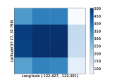
(c) Cabspotting (San Francisco).

Figure 5: The density of users’ spatial regions for the selected area per dataset, which measure $20km*20km$, $20km*20km$, $3.2km*3.2km$ respectively.

6.2 Pre-processing

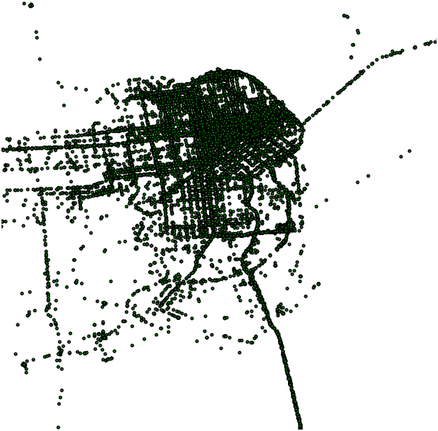
(a)

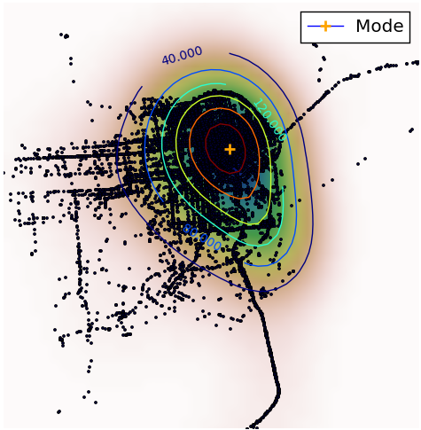
(b)

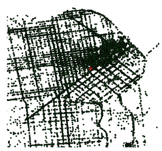
(c)

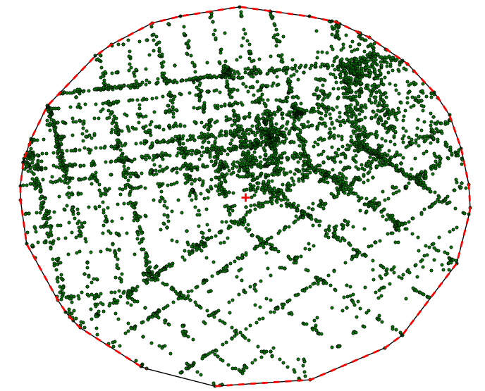
(d)

Figure 6: Pre-processing in experimental setup: Computing the KDE and mode for a set of GPS points, then convex hull. Based on a sample of one cab’s GPS points in San Francisco, from Cabspotting.

We pre-process each dataset to extract convex planar bodies, representing regions where users mostly frequent. This simulates a real application where extraction might be conducted at the end point. For instance, in some applications, e.g., in a fitness tracker, users can determine the area in which they usually locate their workouts, in order to obtain a desired service. We conduct the following steps, which represent just one approach to creating convex regions of high visitation.

• Fit a kernel density estimate (KDE) and consequently take the mode of each user’s set of GPS points;

• Take k-nearest neighbours (k-NN) points to the mode, e.g., for GeoLife, 8 hours corresponds to $k=5760$. If the number of GPS points are less than $k$ we take all points;

• Check if all the points are within the defined $B$ diameter, otherwise discard outliers; and

• Compute the convex hull of remaining points to create a convex planar body representing an area of frequent visitation.

We use standard libraries from the Scipy package Scipy to compute the kNN and convex hull. To deal with geographic coordinates, Euclidean computations do not directly apply, such as to calculate a distance between two points (here: the opposite corners of a bounding box of $B$ diameter). We refer the interested reader to Iliffe2008datums .

Figure 6 demonstrates the trajectory of a cab in San Francisco 6a, taken from the Cabspotting project. In this picture (cf. Figure 6b), the level sets within the contour lines are convex, and we could have picked these for our convex planar body. But in general, level sets are not convex. Our approach generates a convex approximation. As depicted in Figure 6c, cab GPS points in this dataset are dense and concentrated in a specific area. Figure 6d illustrates the extracted convex body.

After pre-processing, we create histogram counts per convex body, to construct the Euler histograms as our baseline approach and as the basis for our other algorithms.

For constrained inference, we used the Gurobi optimisation software package Gurobi which implements dual simplex and barrier algorithms to solve LinProg, with concurrent optimization. We next explain how to choose parameters, then describe our evaluation metrics.

6.3 Parameter Settings

Initial settings for Beijing with four parameters $A$ (area side length), $d$ (cell size), $B$ (bounded diameter), $\epsilon$ are $20km$, $1km$, $2km$ and $1$ respectively. These settings are applied on T-Drive, and GeoLife1.3 datasets. With regard to San Francisco, Cabspotting dataset, area size is $3.2km\times 3.2km$, and cell size is $0.8km$ with the remaining parameters the same. The density of users’ spatial regions per dataset in a selected spatial partition are illustrated in Figure 5. As shown in Figures 5a, 5b, T-Drive and GeoLife reflects a different distribution of users’ spatial regions, and even for the selected area of San Francisco some partitions are more dense, Figure 5c.

Table 2 demonstrates our experimental parameter values, not including the experiments in Sections 6.8–6.10. As demonstrated, bold parameters are varying.

Even though the literature on point data Cormode12PSD ; QardajiYL13 tends to use only specific QR sizes, we vary the QR parameter over the entire range of the area size to more fully evaluate our technique. For experiments where we compare histograms, the $A/d$ ratio, which defines the number of grid cells for each axis, has been kept constant for all datasets (cf. Sections 6.8–6.10).

6.4 Evaluation Metrics

Apart from the varying parameter, we keep all other parameters fixed to compute the median relative error as an empirical measure of utility, as is standard Cormode12PSD ; QardajiYL13 . We repeat each of the experiments 100 times and compute median relative error. The baseline approach is Euler as it provides exact answers. Algorithms DiffPriv, LinProg, Round that are privacy-preserving, are compared to Euler. Another evaluation metric is the percentage of the differences between Euler histograms and the DiffPriv, LinProg, and Round approaches over the difference between Euler histograms and the DiffPriv (relative error to DiffPriv). Here, the $L_{1}$-norm is adopted.

We also compute the number of times each constraint has been violated in each technique compared to LinProg and Round which are the consistent techniques, as well as Euler as our baseline approach, consistency constraints violation. Furthermore, we compute the running time for each algorithm (cf. Section 6.10).

Table 2: Experimental settings. This table shows the range of parameters, bolded are those that are varying.

Dataset	Cell Size (d)	B	Area Size (A)	A/d	QR Size/Shape	$\epsilon$
T-Drive	1km	2km	20km*20km	20	1-10%	1
T-Drive	1km	2km	20km*20km	20	10-100%	1
T-Drive	0.66,1,2km	2km	20km*20km	30,20,10	1%	1
T-Drive	2km	2km	20km*20km	10	1%	0.1,0.4,0.7,1
GeoLife1.3	1km	2km	20km*20km	20	1-10%	1
GeoLife1.3	1km	2km	20km*20km	20	10-100%	1
Cabspotting	0.8km	2km	3.2km*3.2km	4	10-100%	1

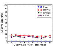
(a) QR Size (1-10% of Total Area).

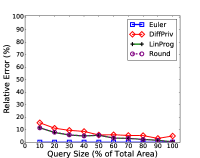
(b) QR Size (10-100% of Total Area).

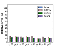
(c) Various QR Shapes (smaller).

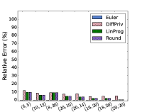
(d) Various QR Shapes (larger).

Figure 7: Median relative error per query size and shape for T-Drive dataset.

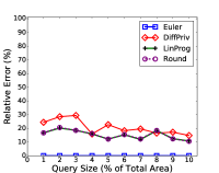
(a) QR Size (1-10% of Total Area).

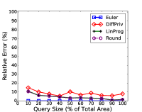
(b) QR Size (10-100% of Total Area).

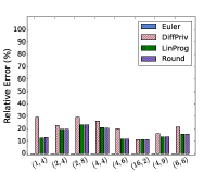
(c) Various QR Shapes (smaller).

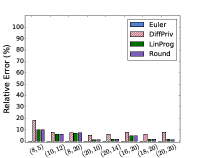
(d) Various QR Shapes (larger).

Figure 8: Median relative error per query size and shape for GeoLife1.3 dataset.

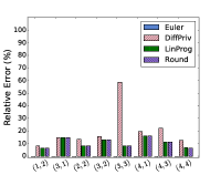
(a) Various QR Shapes.

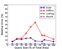
(b) QR Size (10-100% of Total Area).

Figure 9: Median relative error per query size and shape for Cabspotting dataset.

6.5 Varying Query Rectangle Size

In this section we compute the median relative error on all datasets, representing diversity in terms of sparsity, density and concentration, to demonstrate effect on accuracy. We fix every parameter, except QR size to run a range query on various sizes, with varying position on the partitioned map, based on definition of a QR as a union of grid cells. Range queries are varied from 1 to 10 and 10 to 100 percent of the total area size of the respective city. The results for various sizes as well as shapes of a range query are shown in Figures 7–9. Various parameters can affect the response to a QR, including shape of a QR, size of a QR, whether convex bodies are sparse in the space or dense, or if they are concentrated or not. Furthermore, the computed global density (cf. Lemma 2) differs across dataset settings, e.g., $25$ for both T-Drive and GeoLife datasets, and $49$ for Cabspotting, and this value also affects the results. The similarity between T-Drive and Cabspotting is that both record taxi driver movements; but a difference is that the former is not concentrated on a specific area while the latter is. In GeoLife1.3 the convex bodies are more dense, having a large number of trajectories.

As depicted in Figure 7 for the T-Drive dataset, since the data is more evenly distributed the error is very low for larger QR sizes (Figure 7b), and is less than $20\%$ for smaller QRs (Figure 7a). A variety of QR shapes for the smaller sizes (Figure 7c), and larger ones (Figure 7d) are depicted accordingly. For instance, 1% QR in a $20\times 20$ partitioned-map of Beijing city could be $(1,4)$, $(2,2)$, $(4,1)$ geometries, where the first coordinate represents the number of rows and the second represents number of columns. Compared to GeoLife1.3 (Figure 9), since trajectories are more focused on some area (cf. Figure 5b), the error increases by decreasing QR size (Figure 8a).

With regard to the Cabspotting dataset (Figure 9), some parts of the selected area are sparser which consequently affects the result of DiffPriv. Specifically for the QR shape of $(3,3)$ (Figure 9a) and the QR sizes of 50% and 60% (Figure 9b), such QRs contain dense and sparse cells. This results in larger errors. However for larger QRs, errors cancel each other out due to the Euler formula, Equation (1). In all cases, LinProg and Round reduce the errors, and provide a high level of accuracy. Since the number of spatial partitions for the chosen area is smaller than the other datasets, only QR sizes and shapes between 10%–100% are shown in Figures 9a and 9b. The QR errors for the smaller sizes 1%–9% are less than 10%.

LinProg and Round provide similar results, and as discussed in Section 5, the difference is the covertness property of Round. There is inconsistency in the DiffPriv histogram results (see Section 6.9). Providing consistency, through the LinProg and Round techniques, can improve accuracy (cf. Sections 6.6, 6.7).

For the remainder of the experiments for varying other parameters, we focus results on T-Drive dataset, and the 1% QR size as a conservative representative, since it incurs higher error.

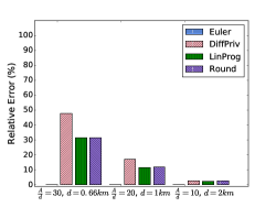
Figure 10: Varying area size/cell size ratio for T-Drive dataset.

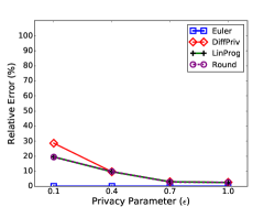
Figure 11: Varying privacy parameter for T-Drive dataset.

6.6 Varying Area Size/Grid Cell Size Ratio

We vary the area size (A) over grid cell size (d) ratio and compute the median relative error for QR taken as 1% of total area of T-Drive dataset. The area size for this dataset is $20km\times 20km$. By increasing the cell size, we expect that the accuracy improves, as demonstrated in Figure 11. We have fixed the QR as 1%, and varied the size of the grid cell in a range 0.66km, 1km, and 2km to yield the ratios of 30, 20, and 10 respectively. As shown, by increasing the grid cell size the accuracy increases. As illustrated in Figure 11, as we decrease the grid cell size, the error increases due to higher values of global sensitivity for smaller cell sizes: $49$, $25$, $9$ are the global sensitivity (GS) values for $0.66km$, $1km$, and $2km$ cell sizes respectively. If we wish to decrease $d$ without incurring reduced accuracy, our theoretical results suggest that we should also decrease $B$ and $A$.

6.7 Varying Privacy Parameter $\epsilon$

We apply a similar procedure to vary the privacy parameter across values 0.1, 0.4, 0.7, and 1 with fixed QR of 1% of the total area $20km\times 20km$, and cell size $2km$. The effect of increasing $\epsilon$ on accuracy is depicted in Figure 11. Decreasing the $\epsilon$ value from $1$, will increase the scale parameter of Laplace distribution (added noise to the counts) from $9$ to $90$ for $\epsilon=0.1$, and this affects the accuracy of the result. To keep accuracy relatively constant when reducing $\epsilon$, the third party can vary other parameters.

6.8 Difference on Histograms

Computing the differences on histograms and their relative error to DiffPriv show that LinProg and Round are superior in terms of having less difference, while still being private. For this part of the experiment, in order to make the dataset histogram differences comparable, we kept the $A/d$ ratio fixed as discussed in Section 6.3, for San Francisco 3.2km/0.16km and for Beijing 20km/1km.

Figure 13 depicts this comparison for all datasets, showing that on the first concentrated dataset, DiffPriv has a considerable difference with LinProg and Round (cf. Cabspotting). This difference decreases for the relatively evenly distributed datasets (cf. GeoLife and T-Drive). LinProg and Round have similar differences with Euler.

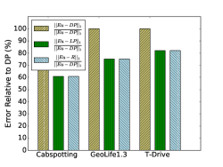
Figure 12: Differences on histograms for all datasets.

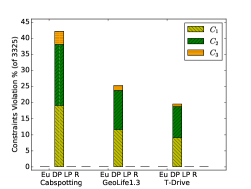
Figure 13: Consistency constrains violations for all datasets.

6.9 Consistency Constraint Violations

In Figure 13 the percentage of violations of constraints $C_{1},C_{2},C_{3}$ is depicted for our datasets. The total number of constraints for each of the datasets is 3325 (as we held $n$ fixed), in which 1520 are for $C_{1}$, 1444 for $C_{2}$ and 361 for $C_{3}$. Approximately the same proportion of the constraints are violated in each dataset, and $C_{3}$ is less than the other constraints, therefore it is not considerably violated. As we decrease the size of the grid cell to 0.16km in Cabspotting, the global sensitivity (cf. Definition 5) increases to 729, therefore it has a greater percentage of violation compared to the other datasets.

6.10 Running Time

Figure 14 shows running times for all datasets of various sizes. As discussed in Section 6.3, we kept the ratio $A/d$ fixed. The running time for all the datasets are approximately similar per technique. The y-axis is in seconds (log-scale) and for the largest dataset GeoLife1.3, the total running time is $\approx$ 196 seconds. DiffPriv, LinProg and Round take less than 1 second for all the datasets. Each of our algorithms are eminently practical to implement and to run.

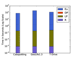
Figure 14: Running time per algorithms for all datasets.

7 Concluding Remarks

For the first time we propose a non-interactive differentially-private approach to counting planar bodies representative of users’ spatial regions e.g., a workout area, areas of customer preference for hotel bookings, or locations of frequent visitation for facility planning.

The key insight of our approach is to leverage Euler histograms for accurate counting, cell perturbations for differential privacy, and constrained inference smoothing to reinstate consistency. Constrained inference often improves utility by cancelling noisy perturbations. Our formulation of constrained inference is a novel constrained application of the robust method of least absolute deviations. Unlike existing constrained inference based on ordinal regression, our formulation precisely matches our privacy-preserving cell perturbation distribution according to maximum-likelihood estimates. By optimising for consistency while rounding cell counts, we achieve a covertness property for our counting mechanism: third parties cannot determine that we have perturbed data in the first place.

A full theoretical analysis of utility and differential privacy is complemented by experimental results on three datasets. As demonstrated in the experimental study, uniformly distributed datasets and larger grid partitions result in a better performance. The best practice to select the cell size is the smallest QR that a third party might run on an area to achieve appropriate utility.

Potential directions for future research include utilising adaptive partitioning to have varying partitions sizes according to the dataset distributions to improve the accuracy. The constraints that we have defined for the Euler histogram counts could be potentially more tight to improve utility. Finally, prior public knowledge about true counts could be incorporated into our constrained inference via regularisation that corresponds to Bayesian priors.

- (1) Ács, G., Castelluccia, C., Chen, R.: Differentially private histogram publishing through lossy compression. In: ICDM’12, pp. 1–10 (2012)
- (2) Andrés, M.E., Bordenabe, N.E., Chatzikokolakis, K., Palamidessi, C.: Geo-indistinguishability: differential privacy for location-based systems. In: CCS’13, pp. 901–914 (2013)
- (3) Barak, B., Chaudhuri, K., Dwork, C., Kale, S., McSherry, F., Talwar, K.: Privacy, accuracy, and consistency too: a holistic solution to contingency table release. In: Proceedings of the Twenty-Sixth ACM SIGACT-SIGMOD-SIGART Symposium on Principles of Database Systems, June 11-13, 2007, Beijing, China, pp. 273–282 (2007)
- (4) Beigel, R., Tanin, E.: The geometry of browsing. In: LATIN ’98: Theoretical Informatics, Third Latin American Symposium, pp. 331–340 (1998)
- (5) Beresford, A.R., Stajano, F.: Location privacy in pervasive computing. IEEE Pervasive Computing 2(1), 46–55 (2003)
- (6) Braz, F., Orlando, S., Orsini, R., Raffaetà, A., Roncato, A., Silvestri, C.: Approximate aggregations in trajectory data warehouses. In: Proceedings of the 23rd International Conference on Data Engineering Workshops, ICDE 2007, pp. 536–545 (2007)
- (7) Chawla, S., Dwork, C., McSherry, F., Talwar, K.: On the utility of privacy-preserving histograms. In: Proceedings of the 21st Conference on Uncertainty in Artificial Intelligence (2005)
- (8) Chen, R., Fung, B.C.M., Desai, B.C., Sossou, N.M.: Differentially private transit data publication: a case study on the Montreal transportation system. In: KDD’12, pp. 213–221 (2012)
- (9) Chow, C.Y., Mokbel, M.F.: Privacy of spatial trajectories. In: Y. Zheng, X. Zhou (eds.) Computing with Spatial Trajectories, pp. 109–141. Springer (2011)
- (10) Chow, C.Y., Mokbel, M.F.: Trajectory privacy in location-based services and data publication. SIGKDD Explorations 13(1), 19–29 (2011)
- (11) Cormode, G., Procopiuc, C.M., Srivastava, D., Shen, E., Yu, T.: Differentially private spatial decompositions. In: ICDE’12, pp. 20–31 (2012)
- (12) Dielman, T.E.: Least absolute value regression: recent contributions. Journal of Statistical Computation and Simulation 75(4), 263–286 (2005)
- (13) Dwork, C.: Differential privacy: A survey of results. In: Theory and Applications of Models of Computation, 5th International Conference, TAMC, pp. 1–19 (2008)
- (14) Dwork, C.: A firm foundation for private data analysis. Communications of the ACM 54(1), 86–95 (2011)
- (15) Dwork, C., McSherry, F., Nissim, K., Smith, A.: Calibrating noise to sensitivity in private data analysis. In: Theory of Cryptography, Third Theory of Cryptography Conference, TCC, Lecture Notes in Computer Science, vol. 3876, pp. 265–284. Springer (2006)
- (16) Fan, L., Xiong, L., Sunderam, V.S.: Differentially private multi-dimensional time series release for traffic monitoring. In: IFIP’13. Proceedings, pp. 33–48 (2013)
- (17) Fanaeepour, M., Kulik, L., Tanin, E., Rubinstein, B.I.P.: The CASE histogram: privacy-aware processing of trajectory data using aggregates. GeoInformatica 19(4), 747–798 (2015)
- (18) Fanaeepour, M., Rubinstein, B.I.P.: Beyond points and paths: Counting private bodies. In: ICDM, pp. 131–140 (2016)
- (19) Ghinita, G.: Privacy for location-based services. In: E. Bertino, R. Sandhu (eds.) Privacy for Location-based Services, Synthesis Lectures on Information Security, Privacy, and Trust. Morgan & Claypool Publishers (2013)
- (20) Gruteser, M., Liu, X.: Protecting privacy in continuous location-tracking applications. IEEE Security & Privacy 2(2), 28–34 (2004)
- (21) Gurobi Optimization, Inc.: Gurobi optimizer reference manual (2015). URL http://www.gurobi.com
- (22) Hay, M., Rastogi, V., Miklau, G., Suciu, D.: Boosting the accuracy of differentially private histograms through consistency. PVLDB 3(1), 1021–1032 (2010)
- (23) He, X., Cormode, G., Machanavajjhala, A., Procopiuc, C.M., Srivastava, D.: DPT: differentially private trajectory synthesis using hierarchical reference systems. PVLDB 8(11), 1154–1165 (2015)
- (24) Hsu, J., Gaboardi, M., Haeberlen, A., Khanna, S., Narayan, A., Pierce, B.C., Roth, A.: Differential privacy: An economic method for choosing epsilon. In: IEEE 27th Computer Security Foundations Symposium, CSF 2014, pp. 398–410 (2014)
- (25) Iliffe, J., Lott, R.: Datums and map projections for remote sensing, GIS and surveying. Whittles Publishing (2008). URL https://books.google.com.au/books?id=u\_4RAQAAIAAJ
- (26) Inan, A., Kantarcioglu, M., Ghinita, G., Bertino, E.: Private record matching using differential privacy. In: EDBT’10, pp. 123–134 (2010)
- (27) Jones, E., Oliphant, T., Peterson, P., et al.: SciPy: Open source scientific tools for Python (2001–). URL http://www.scipy.org/
- (28) Karmarkar, N.: A new polynomial-time algorithm for linear programming. In: STOC’84, pp. 302–311 (1984)
- (29) Kifer, D., Lin, B.: Towards an axiomatization of statistical privacy and utility. In: Proceedings of the Twenty-Ninth ACM SIGMOD-SIGACT-SIGART Symposium on Principles of Database Systems, PODS, pp. 147–158 (2010)
- (30) Krumm, J.: Inference attacks on location tracks. In: 5th International Conference on Pervasive Computing, PERVASIVE’07, pp. 127–143 (2007)
- (31) Krumm, J.: A survey of computational location privacy. Personal and Ubiquitous Computing 13(6), 391–399 (2009)
- (32) Leonardi, L., Orlando, S., Raffaetà, A., Roncato, A., Silvestri, C., Andrienko, G.L., Andrienko, N.V.: A general framework for trajectory data warehousing and visual OLAP. GeoInformatica 18(2), 273–312 (2014)
- (33) Li, C., Hay, M., Miklau, G., Wang, Y.: A data- and workload-aware query answering algorithm for range queries under differential privacy. PVLDB 7(5), 341–352 (2014)
- (34) López, I.F.V., Snodgrass, R.T., Moon, B.: Spatiotemporal aggregate computation: a survey. IEEE Transactions on Knowledge and Data Engineering, TKDE 17(2), 271–286 (2005)
- (35) Marketos, G., Frentzos, E., Ntoutsi, I., Pelekis, N., Raffaetà, A., Theodoridis, Y.: Building real-world trajectory warehouses. In: Seventh ACM International Workshop on Data Engineering for Wireless and Mobile Access, Mobide 2008, pp. 8–15 (2008)
- (36) Mir, D.J., Isaacman, S., Cáceres, R., Martonosi, M., Wright, R.N.: DP-WHERE: differentially private modeling of human mobility. In: Proceedings of the 2013 IEEE International Conference on Big Data, pp. 580–588 (2013)
- (37) Papadias, D., Kalnis, P., Zhang, J., Tao, Y.: Efficient OLAP operations in spatial data warehouses. In: 7th International Symposium on Advances in Spatial and Temporal Databases, SSTD’01, pp. 443–459 (2001)
- (38) Papadias, D., Tao, Y., Kalnis, P., Zhang, J.: Indexing spatio-temporal data warehouses. In: Proceedings of the 18th International Conference on Data Engineering, ICDE’02, pp. 166–175 (2002)
- (39) Piorkowski, M., Sarafijanovoc-Djukic, N., Grossglauser, M.: A Parsimonious Model of Mobile Partitioned Networks with Clustering. In: COMSNETS (2009). URL http://www.comsnets.org
- (40) Primault, V., Mokhtar, S.B., Lauradoux, C., Brunie, L.: Differentially private location privacy in practice. CoRR abs/1410.7744 (2014)
- (41) Qardaji, W.H., Yang, W., Li, N.: Differentially private grids for geospatial data. In: ICDE’13, pp. 757–768 (2013)
- (42) Rubinstein, B.I.P., Bartlett, P.L., Huang, L., Taft, N.: Learning in a large function space: Privacy-preserving mechanisms for SVM learning. J. Privacy and Confidentiality 4(1), 65–100 (2012)
- (43) Sun, C., Agrawal, D., El Abbadi, A.: Exploring spatial datasets with histograms. In: Proceedings of the 18th International Conference on Data Engineering, ICDE, pp. 93–102 (2002)
- (44) Sun, C., Agrawal, D., El Abbadi, A.: Selectivity estimation for spatial joins with geometric selections. In: EDBT’02, pp. 609–626 (2002)
- (45) Sun, C., Bandi, N., Agrawal, D., El Abbadi, A.: Exploring spatial datasets with histograms. Distributed and Parallel Databases 20(1), 57–88 (2006)
- (46) Tao, Y., Kollios, G., Considine, J., Li, F., Papadias, D.: Spatio-temporal aggregation using sketches. In: Proceedings of the 20th International Conference on Data Engineering, ICDE 2004, pp. 214–225 (2004)
- (47) Tao, Y., Papadias, D., Zhang, J.: Aggregate processing of planar points. In: 8th International Conference on Extending Database Technology, EDBT 2002, pp. 682–700 (2002)
- (48) Timko, I., Böhlen, M.H., Gamper, J.: Sequenced spatio-temporal aggregation in road networks. In: EDBT 2009, 12th International Conference on Extending Database Technology, pp. 48–59 (2009)
- (49) To, H., Ghinita, G., Shahabi, C.: A framework for protecting worker location privacy in spatial crowdsourcing. PVLDB 7(10), 919–930 (2014)
- (50) Trudeau, R.: Introduction to Graph Theory. Dover Books on Mathematics Series. Dover Pub. (1993)
- (51) Wang, M., Zhang, X., Meng, X.: DiffR-tree: A differentially private spatial index for OLAP query. In: WAIM’13, pp. 705–716 (2013)
- (52) Xie, H., Tanin, E., Kulik, L.: Distributed histograms for processing aggregate data from moving objects. In: 8th International Conference on Mobile Data Management (MDM 2007), pp. 152–157 (2007)
- (53) Xie, H., Tanin, E., Kulik, L., Scheuermann, P., Trajcevski, G., Fanaeepour, M.: Euler histogram tree: A spatial data structure for aggregate range queries on vehicle trajectories. In: 7th ACM SIGSPATIAL International Workshop on Computational Transportation Science, IWCTS 2014 (2014)
- (54) Yuan, J., Zheng, Y., Zhang, C., Xie, W., Xie, X., Sun, G., Huang, Y.: T-drive: driving directions based on taxi trajectories. In: 18th ACM SIGSPATIAL International Symposium on Advances in Geographic Information Systems, ACM-GIS 2010, pp. 99–108 (2010)
- (55) Zhang, J., Ghinita, G., Chow, C.: Differentially private location recommendations in geosocial networks. In: MDM’14, pp. 59–68 (2014)
- (56) Zheng, Y., Xie, X., Ma, W.: Geolife: A collaborative social networking service among user, location and trajectory. IEEE Data Engineering Bulletin 33(2), 32–39 (2010)