Does the configurational entropy of polydisperse particles exist?

Abstract

Classical particle systems characterized by continuous size polydispersity, such as colloidal materials, are not straightforwardly described using statistical mechanics, since fundamental issues may arise from particle distinguishability. Because the mixing entropy in such systems is divergent in the thermodynamic limit we show that the configurational entropy estimated from standard computational approaches to characterize glassy states also diverges. This reasoning would suggest that polydisperse materials cannot undergo a glass transition, in contradiction to experiments. We explain that this argument stems from the confusion between configurations in phase space and states defined by free energy minima, and propose a simple method to compute a finite and physically meaningful configurational entropy in continuously polydisperse systems. Physically, the proposed approach relies on an effective description of the system as an $M^{*}$-component system with a finite $M^{*}$, for which finite mixing and configurational entropies are obtained. We show how to directly determine $M^{*}$ from computer simulations in a range of glass-forming models with different size polydispersities, characterized by hard and soft interparticle interactions, and by additive and non-additive interactions. Our approach provides consistent results in all cases and demonstrates that the configurational entropy of polydisperse system exists, is finite, and can be quantitatively estimated.

I Configurational entropy in polydisperse systems

Colloidal systems play an important role in a wide spectrum of soft condensed matter physics, from crystallization kinetics to the glass transition phenomenon. An important motivation is that colloids can be seen as “big atoms”, which may prove useful in terms of microscopic observations and particle design Poon (2004). These colloidal particles are composed of a very large number of atoms, such that each colloid in a given experimental batch is a unique object. Therefore, colloidal particles are distinguishable classical objects, which rises subtle theoretical issues for their statistical mechanical treatment Cates and Manoharan (2015). In particular, colloidal particles are often characterized by a continuous distribution $f(\sigma)$ of particle diameters, $\sigma$. Thus, in principle, colloids can be readily distinguished by their sizes and there are no two identical particles in the system. Polydisperse systems are widely employed in studies of the glass transition because polydispersity efficiently prevents crystallization. Therefore, understanding how polydispersity impacts the theoretical treatment of glass formation is an important question that constitutes the main theme of this paper.

The statistical mechanics of continuously polydisperse systems has been widely studied in a number of contexts Salacuse and Stell (1982); Briano and Glandt (1984); Warren (1998); Sollich and Cates (1998); Sollich (2001). Particle distinguishability may cause in particular some subtle issues, such as the well-known Gibbs paradox Swendsen (2008) and this requires special attention Cates and Manoharan (2015). In that case, particle indistinguishability stemming from a quantum mechanical treatment cannot be invoked for colloidal particles Frenkel (2014).

Before proceeding to our discussion of disordered materials, let us recall what happens in the case of ordered materials. In a recent article, Cates and Manoharan discuss the existence of a colloidal crystal made of weakly polydisperse hard spheres Cates and Manoharan (2015): “In the fluid, the spheres can easily swap places whereas in the crystal, they cannot. For indistinguishable particles, the entropy gain on transforming from liquid to crystal is extensive. The additional entropy cost of localizing distinguishable particles onto un-swappable lattice sites contains a term $k_{\rm B}\ln(N!)$ where $N!$ counts particle permutations. This term must be paid to collapse an accessible phase-space volume in which distinguishable particles can change places, into one where they cannot. This putative entropy cost is supra-extensive ($k_{\rm B}N\ln N$) and thus for large $N$ outweighs the extensive entropy on formation of the crystal. Thus the kinetic approach to entropy predicts that colloidal crystals are thermodynamically impossible. Yet they are observed every day.” This paradox is resolved by including the $N!$ distinct crystal configurations generated by the permutation of $N$ distinguishable particles in a single crystalline state. Then, this $N!$ multiplicity term cancels exactly the putative entropy cost due to particle distinguishability Cates and Manoharan (2015). Physically, this theoretical treatment corresponds to describing the polydisperse system as behaving effectively as a one-component system and it highlights the conceptual difference between configurations in phase space volume and states defined from free energy minima, which are usually constructed from a much larger number of configurations. These basic ideas will reappear throughout our discussion of disordered materials.

Another well-known issue arising in continuously polydisperse systems is the divergence of the mixing entropy, $S_{\rm mix}$ Salacuse and Stell (1982); Zhang et al. (1999); Frenkel (2014). Mathematically, this is because the mixing entropy of a discrete mixture of particles diverges in the limit of an infinite number of components, which is needed to formally represent a continuous distribution in the thermodynamic limit. In several situations, this divergent contribution is immaterial, for instance when discussing phase equilibria with a fixed particle size distribution $f(\sigma)$ Sollich (2001) or mixing processes of two different continuous polydisperse systems Paillusson and Pagonabarraga (2014), because the absolute value of the entropy is irrelevant and only entropy differences between two systems matter Barrat and Hansen (1986); Sollich (2001); Paillusson and Pagonabarraga (2014); Frenkel (2014). In the above-mentioned cases, the diverging contributions to $S_{\rm mix}$ cancel each other.

All these issues are relevant for a proper treatment of the glass transition in polydisperse materials, but this has never been carefully discussed before. The configurational entropy $S_{\rm conf}$ is the central quantity to describe the thermodynamics of supercooled liquids approaching the glass transition Kauzmann (1948); Adam and Gibbs (1965); Berthier and Biroli (2011). Conventionally in computer simulations (and also in experiments), $S_{\rm conf}$ is defined as $S_{\rm conf}=S_{\rm tot}-S_{\rm vib}$, where $S_{\rm tot}$ is the total entropy of the system and $S_{\rm vib}$ is the entropy of the glass (or vibrational) state where only particle vibrations due to thermal fluctuations take place Kauzmann (1948); Adam and Gibbs (1965); Berthier and Biroli (2011). Physically, $S_{\rm conf}$ quantifies the number of available amorphous states in glassy systems. These metastable states are understood as long-lived free energy minima Berthier and Biroli (2011), even though their mathematical definition in finite dimensional glass models remains problematic Biroli and Kurchan (2001). The mean-field theory of the glass transition is based on the existence of an ideal glass transition occurring at temperature $T_{\rm K}$ at which $S_{\rm conf}$ vanishes Charbonneau et al. (2014). Hence, there is a need for a careful investigation of the entropy of polydisperse glassy materials.

An extension of the argument developed by Cates and Manoharan for the polydisperse crystal Cates and Manoharan (2015) can be made for the configurational and mixing entropies of a polydisperse glass. In that case, the system transforms from the fluid where particle swaps are easy to the glass where they are not. In multi-component glass-formers, the entropy of the fluid state must contain a mixing entropy contribution $S_{\rm mix}$, because the particles can exchange their positions Coluzzi et al. (1999); Sciortino, Kob, and Tartaglia (1999); Sastry (2000); Angelani and Foffi (2007). It is conventionally assumed that $S_{\rm vib}$ does not contain the mixing contribution Sciortino (2005), because particles in the glass state mainly vibrate around a fixed averaged position in a given glass configuration and particle exchanges are neglected. Pushing further this argument, the divergence of $S_{\rm mix}$ for continuous polydispersity provokes the divergence of the entropy of the fluid, whereas the glass entropy remains finite. Logically, then, if the configurational entropy is infinite in the fluid, it cannot vanish and the glass transition cannot exist. This reasoning is of course in direct contradiction with experiments and simulations, where “polydisperse glasses are observed every day”, to paraphrase Cates and Manoharan.

The goal of this paper is to provide a conceptually-correct and computationally-simple way to define and measure the configurational entropy in continuously polydisperse systems. There exist many separate studies of the glassy behavior of colloidal and polydisperse systems both in experiments Hunter and Weeks (2012); Gokhale, Sood, and Ganapathy (2016) and simulations Santen and Krauth (2000); Brumer and Reichman (2004); Kawasaki, Araki, and Tanaka (2007); Hermes and Dijkstra (2010); Zaccarelli, Liddle, and Poon (2015) and of the configurational entropy in glass-forming models Speedy (1993); Sciortino, Kob, and Tartaglia (1999); Sastry (2001); Angelani and Foffi (2007); Berthier and Coslovich (2014); Asenjo, Paillusson, and Frenkel (2014); Martiniani et al. (2016); Vink and Barkema (2002); Anikeenko, Medvedev, and Aste (2008); Zhou and Milner (2016); Ronceray and Harrowell (2016). However, we are not aware of any detailed theoretical or numerical treatment of the configurational entropy for continuously polydisperse systems, for which standard methods are not valid, as we just showed. Our paper thus fills this gap.

Our basic idea is to treat a continuously polydisperse system as an effective $M^{*}$-component system with a finite number of components $M^{*}$, which can take real values. Within this approach, the glass entropy then also contains a diverging contribution which cancels the one in the total entropy $S_{\rm tot}$. In other words, we estimate a finite and physically-relevant contribution to the mixing entropy, which we call an effective mixing entropy $S_{\rm mix}^{*}$. As a result, we obtain a finite estimate for the configurational entropy $S_{\rm conf}$ as well. This treatment thus shows that the configurational entropy of polydisperse systems is always finite, and may possibly vanish at a glass transition. In addition, we propose a numerical method to determine $M^{*}$ and $S_{\rm mix}^{*}$, which is generically applicable to any glass-forming computer model.

Before closing this introduction, we need to mention that recently, an alternative method to compute the configurational entropy was proposed Berthier and Coslovich (2014), which is based on the Franz-Parisi construction Franz and Parisi (1997). In this approach, the configurational entropy is estimated as a free energy difference, and it is measured in monodisperse and polydisperse systems in the exact same way. Thus, this method automatically produces finite values of the configurational entropy without suffering from a divergent mixing entropy. Results using this method for a continuous polydisperse system have only very recently been obtained Berthier et al. (2016a). Because this approach is numerically more demanding than the standard ones discussed in this paper, it is useful to make the latter applicable to polydisperse systems, such that both types of methods can be compared.

The paper is organized as follows. In Sec. II, we propose our theoretical idea to compute the configurational entropy in continuous polydisperse system. In Sec. III, we describe the numerical method to determine $M^{*}$ and $S_{\rm mix}^{*}$. In Sec. IV, we validate our approach for several simulation models. In Sec. V, we provide a discussion of our results together with some perspectives.

II Theoretical considerations: The main problem and its physical resolution

In this section, we present our approach to compute the configurational entropy in continuously polydisperse systems. We first fix the notations and give some definitions. We then introduce a simple theoretical model of a binary mixture illustrating the core problem to be faced. Through the discussion and resolution of the paradoxical results obtained in this simple model, we draw more general conclusions which lead to our simple proposal to analyze the configurational entropy of generic polydisperse systems.

II.1 Mixing entropy in polydisperse systems

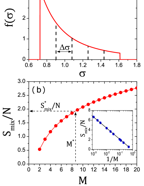
Figure 1: (a) Particle size distribution $f(\sigma)=A\sigma^{-3}$ for $\sigma\in[\sigma_{\rm min},\sigma_{\rm max}]$, $f(\sigma)=0$ outside this range. The dashed lines illustrate the decomposition of $f(\sigma)$ into the arbitrary example of $M=5$ species, with $\Delta\sigma=(\sigma_{\rm max}-\sigma_{\rm min})/M$. (b) The mixing entropy $S_{\rm mix}$ computed from Eqs. (5, 8). The dashed arrows define the value of $S_{\rm mix}^{*}$ from an effective value $M^{*}$. The inset demonstrates the logarithmic divergence of $S_{\rm mix}/N$ when $M\to\infty$.

We first provide definitions and notations related to the statistical mechanics and mixing entropy in mixtures of particles. We consider a continuously polydisperse system whose particle size distribution is given by $f(\sigma)$. To derive the mixing entropy of this system, we decompose $f(\sigma)$ into an integer number $M$ of species Salacuse and Stell (1982); Zhang et al. (1999); Frenkel (2014), as illustrated in Fig. 1(a) for a specific example. The continuously polydisperse system is recovered in the limit $M\to\infty$.

We consider the canonical ensemble characterized by the number of particles $N$, the volume $V$, and the temperature $T=1/\beta$. We set the Boltzmann constant to unity. The partition function $Z_{\rm tot}$ of the system is

$$Z_{\rm tot}=\frac{1}{\Pi_{m=1}^{M}N_{m}!\Lambda^{dN}}\int_{V}\mathrm{d}{\bf r}^{N}e^{-\beta U({\bf r}^{N})},$$ (1)

where $\Lambda$, $d$, and $U$ are the de Broglie thermal wavelength, spatial dimension, and potential energy, respectively. For simplicity, we consider equal masses (hence equal $\Lambda$) irrespective of species throughout this paper. $N_{m}$ is the number of particles within species $m$, such that $N=\sum_{m=1}^{M}N_{m}$. Note that the term, $1/\Pi_{m=1}^{M}N_{m}!$ (or more simply $1/N!$ when $m=1$), should be included irrespective of distinguishability of the particles in order to obtain an extensive free energy Warren (1998); Swendsen (2008); Frenkel (2014); Cates and Manoharan (2015) (see also recent numerical verifications in Refs. Asenjo, Paillusson, and Frenkel, 2014; Martiniani et al., 2016). The total free energy of the system is

$$\beta F_{\rm tot}=-\ln Z_{\rm tot}.$$ (2)

Then, the total entropy $S_{\rm tot}$ can be written as

$$S_{\rm tot}=\beta(E_{\rm tot}-F_{\rm tot})\sim\ln Z_{\rm tot}\sim-\ln(\Pi_{m=1}^{M}N_{m}!),$$ (3)

where $E_{\rm tot}$ is the total energy of the system. In this paper, we use the symbol “$\sim$” to single out the contribution due to the mixing entropy. Instead, we use the symbol “$\simeq$” to express the conventional “nearly equal” relation. By applying Stirling’s approximation, $\ln x!\simeq x\ln x-x$ ($x\gg 1$), we get

$$\ln(\Pi_{m=1}^{M}N_{m}!)\simeq(N\ln N-N)+N\sum_{m=1}^{M}X_{m}\ln X_{m},$$ (4)

where $X_{m}=N_{m}/N$ is the concentration of species $m$. The second term in Eq. (4) comes from the effect of having a system with $M$ components, i.e., from the size polydispersity. The mixing entropy $S_{\rm mix}^{(M)}$ is defined as

$$S_{\rm mix}^{(M)}=-N\sum_{m=1}^{M}X_{m}\ln X_{m}.$$ (5)

For latter purposes, we note that the mixing entropy provides a contribution to the total entropy $S_{\rm tot}$. Using the ‘$\sim$’ notation introduced above, we have

$$S_{\rm tot}\sim S_{\rm mix}^{(M)}.$$ (6)

We can clearly see that in a continuously polydisperse case, when we have $M=N$ and hence $X_{m}=1/N$, the mixing entropy $S_{\rm mix}^{(M)}$ diverges in the thermodynamic limit, $N\to\infty$,

$$\frac{S_{\rm mix}^{(M=N)}}{N}=-\sum_{m=1}^{N}\frac{1}{N}\ln\frac{1}{N}=\ln N\xrightarrow[N\to\infty]{}\infty.$$ (7)

Alternatively, if we represent a system characterized by a continuous size distribution $f(\sigma)$ as an $M$-component mixture, then we divide the distribution into $M$ equal intervals, $\Delta\sigma=(\sigma_{\rm max}-\sigma_{\rm min})/M$, see Fig. 1(a) for an example. Therefore we have

$$X_{m}=\int_{\sigma_{m}}^{\sigma_{m+1}}\mathrm{d}\sigma f(\sigma),$$ (8)

where $\sigma_{m}=\sigma_{\rm min}+(m-1)\Delta\sigma$. Using Eqs. (5) and (8), we get $S_{\rm mix}$ as a function of $M$. In Fig. 1(b), we show $S_{\rm mix}^{(M)}$ for a specific example of $f(\sigma)$ which will be studied numerically below. In the inset of Fig. 1(b), we confirm that $S_{\rm mix}/N$ diverges logarithmically in the continuous polydisperse limit, $M\to\infty$ (or $\Delta\sigma\to 0$) Salacuse and Stell (1982); Zhang et al. (1999); Frenkel (2014), as expected.

Note that in Refs. Salacuse and Stell, 1982; Zhang et al., 1999; Frenkel, 2014, a formal expression of the continuous polydisperse limit is given by

$$\lim_{M\to\infty}\frac{S_{\rm mix}^{(M)}}{N} = -\lim_{\begin{subarray}{c}M\to\infty\\ \Delta\sigma\to 0\end{subarray}}\sum_{m=1}^{M}f(\sigma_{m})\Delta\sigma\ln(f(\sigma_{m})\Delta\sigma)$$ (9)

$$= -\int_{0}^{\infty}\mathrm{d}\sigma f(\sigma)\ln f(\sigma)-\lim_{\Delta\sigma\to 0}\ln\Delta\sigma.$$

In this expression, the divergent mixing entropy is decomposed into a finite term depending on $f(\sigma)$ (the first term) and a divergent term (the second term) in Eq. (9). However, the first term is not a well-defined quantity, since it depends on the argument or labeling of the distribution $f$ Zhang et al. (1999), and hence one cannot use the first term alone for a physically relevant mixing entropy to compute the configurational entropy.

II.2 A paradox for binary mixtures

We introduce a simple model of a glass-forming binary mixture whose analysis produces paradoxical results that illustrate the core of the problem that we face regarding the mixing entropy of polydisperse particles. The physics of this system has been discussed qualitatively in Ref. Coluzzi et al., 1999.

We consider a binary mixture ($M=2$) composed of species 1 and 2 in arbitrary dimensions. The diameters of the particles are respectively $\sigma_{\rm 1}=\sigma$ and $\sigma_{\rm 2}=\sigma(1+\epsilon)$, with $\epsilon>0$. For simplicity, we consider equal concentrations, $X_{1}=X_{2}=1/2$. In this setting, the total entropy $S_{\rm tot}$ always contains the mixing entropy $S_{\rm mix}$ irrespective of the absolute value of $\epsilon$, so that the mixing contribution to the total entropy reads

$$S_{\rm tot}\sim S_{\rm mix}=N\ln 2.$$ (10)

In previous studies of binary mixtures with $\epsilon\simeq 1$, this mixing entropy term was included to compute the configurational entropy and to detect the ideal glass transition Speedy (1998); Sciortino, Kob, and Tartaglia (1999); Coluzzi et al. (1999); Sastry (2000); Angelani and Foffi (2007); Ozawa et al. (2015). However, the fact that the mixing entropy does not depend on $\epsilon$ is quite surprising. Indeed, when $\epsilon\ll 1$, one can expect that the physics of such a nearly monodisperse system should not be very different from that of purely one-component system obtained by setting $\epsilon=0$. In particular, the ideal glass transition temperature $T_{\rm K}$ (or density $\phi_{\rm K}$ for hard spheres) of this binary system, if it exists, should not be very different from that of the purely one-component system. More precisely, one would expect that $T_{K}$ is a continuous function of $\epsilon$ near $\epsilon=0$. However, the configurational entropy $S_{\rm conf}/N$ of the binary system is larger than that of the purely one-component system by $\ln 2\simeq 0.7$, due to the mixing entropy contribution in Eq. (10), and this large entropy appears discontinuously as soons as $\epsilon>0$. The theoretical analysis of this system is therefore physically inconsistent.

One possible solution to the paradox would be to always neglect the mixing entropy contribution, as done for instance in Ref. Biazzo et al., 2009. However, such treatment would change the location of the ideal glass transition significantly. Let us consider two examples to illustrate this point. In the Kob-Andersen (KA) model Kob and Andersen (1995), the mixing entropy contributes $S_{\rm mix}/N\simeq 0.5$ to the total entropy $S_{\rm tot}$ Sciortino, Kob, and Tartaglia (1999). If one neglects $S_{\rm mix}/N$ from $S_{\rm conf}/N$, the estimated $T_{\rm K}\simeq 0.3$ Sciortino, Kob, and Tartaglia (1999); Sastry (2000); Ozawa et al. (2015) increases to $T_{\rm K}\simeq 0.5$, a temperature that is actually easily equilibrated in the simulations Kob and Andersen (1995). In the binary hard sphere model studied in Ref. Angelani and Foffi, 2007, one has $S_{\rm mix}/N=\ln 2\simeq 0.693$ Angelani and Foffi (2007). If one again removes $S_{\rm mix}/N$, the estimated ideal glass transition density, $\phi_{\rm K}\simeq 0.62$ Angelani and Foffi (2007), is now reduced to $\phi_{\rm K}\simeq 0.58$, where equilibrium is again easily achieved Angelani and Foffi (2007). Assuming that the other contributions to the numerical estimate of $S_{\rm conf}$ are well-controlled, then it appears impossible to neglect the mixing entropy.

These examples demonstrate that the mixing entropy term is actually needed for a proper estimate of the configurational entropy. But if so, then it must be included in any binary mixture, including one where $\epsilon\ll 1$. But in that case the limit $\epsilon\to 0$ produces a jump in the estimated location of the glass transition, which is unphysical.

In summary, when considering our simple example of a binary mixture with size ratio $(1+\epsilon)$, taking $\epsilon$ as a continuous parameter suggests that previous approaches to determine the configurational entropy cannot be applied directly, as one needs to decide a priori whether or not to include the mixing entropy in the configurational entropy. Such decision can still produce meaningful results when $\epsilon$ is a constant which is either large enough or very small. But when intermediate $\epsilon$ values are considered, or when the particle size distribution becomes more complex, an adhoc approach becomes impossible. Importantly for the present work, this approach breaks down completely when the polydispersity becomes continuous, because then a continuous spectrum of large and small $\epsilon$ values coexists in a single system.

II.3 Physical resolution of the binary mixture paradox

To resolve the above paradox, we carefully discuss the vibrational (or glass) state and its entropy. We suppose that the equilibrium system is sufficiently deeply supercooled that there is a strong separation of timescales between vibrations and structural relaxation. This implies that it makes sense to consider a vibrational state.

To compute the vibrational entropy $S_{\rm vib}$, one must evaluate the partition function of this vibrational state, $Z_{\rm vib}$, by performing a configurational integral within the restricted phase space volume $V_{\rm basin}$ explored by the system over the vibrational timescale. To perform the configurational integral, a representative basin, denoted by $\alpha$, is randomly selected and then the configurational integral is evaluated numerically using methods such as the harmonic approximation around the local minimum of the potential energy Sciortino, Kob, and Tartaglia (1999); Sastry (2000), or a Frenkel-Ladd Frenkel and Ladd (1984) thermodynamic integration over a system constrained by harmonic springs Coluzzi et al. (1999); Sastry (2000); Angelani and Foffi (2007).

However, there is a factorial degeneracy of $\alpha$ in the phase space volume. In particular, these basins can be generated by permutation of the particles Cates and Manoharan (2015). Thus, we have to take into account the number of physically identical basins to evaluate $Z_{\rm vib}$. When $\epsilon\simeq 1$ (corresponding to typical binary mixtures Sciortino, Kob, and Tartaglia (1999); Angelani and Foffi (2007)), the multiplicity is simply given by the number of configurations obtained by permuting particles within each species (1 $\leftrightarrow$ 1 or 2 $\leftrightarrow$ 2), and this corresponds to $N_{\rm 1}!N_{\rm 2}!$. Instead, when $\epsilon\ll 1$, the permutation of particles between unlike species (1 $\leftrightarrow$ 2) should also be taken into account, because this manipulation also generates configurations belonging to the physically identical basin.

Thus, we need to multiply the configurational integral by $N!$ instead of $N_{\rm 1}!N_{\rm 2}!$. As a result, $Z_{\rm vib}$ is different in the two cases, $\epsilon\simeq 1$ and $\epsilon\ll 1$, as follows,

$$Z_{\rm vib}=\left\{\begin{aligned} \quad&\frac{N_{\rm 1}!N_{\rm 2}!}{N_{\rm 1}!N_{\rm 2}!\Lambda^{dN}}\int_{V_{\rm basin}}\mathrm{d}{\bf r}^{N}e^{-\beta U({\bf r}^{N})}\quad\left(\epsilon\simeq 1\right),\\ \quad&\frac{N!}{N_{\rm 1}!N_{\rm 2}!\Lambda^{dN}}\int_{V_{\rm basin}}\mathrm{d}{\bf r}^{N}e^{-\beta U({\bf r}^{N})}\quad\left(\epsilon\ll 1\right).\end{aligned}\right.$$ (11)

Therefore, the vibrational entropy contains a mixing entropy contribution whose value depends explicitly on the value of $\epsilon$,

$$S_{\rm vib}\sim\ln Z_{\rm vib}\sim\left\{\begin{aligned} \quad&0\qquad\left(\epsilon\simeq 1\right)\\ \quad&N\ln 2\qquad\left(\epsilon\ll 1\right).\end{aligned}\right.$$ (12)

When $\epsilon\simeq 1$, the vibrational entropy does not contain a finite mixing entropy, which is consistent with previous studies Sciortino, Kob, and Tartaglia (1999); Angelani and Foffi (2007). However, when $\epsilon\ll 1$, the vibrational entropy contains a mixing entropy contribution, which originates from the fact that particles with similar (but distinct) sizes can be permuted within the vibrational state. By combining Eqs. (10, 12), we obtain $S_{\rm conf}$ as,

$$S_{\rm conf}=S_{\rm tot}-S_{\rm vib}\sim\left\{\begin{aligned} \quad&N\ln 2\qquad\left(\epsilon\simeq 1\right)\\ \quad&0\qquad\left(\epsilon\ll 1\right).\end{aligned}\right.$$ (13)

In this reasoning, the mixing entropy contribution to $S_{\rm vib}$ for $\epsilon\ll 1$ exactly cancels the one in $S_{\rm tot}$ and thus $S_{\rm conf}$ does not contain any mixing entropy, which is consistent with the physics of a purely one-component system. As a result, $T_{\rm K}$ would not change discontinuously between $\epsilon\ll 1$ and the purely one-component system with $\epsilon=0$, thus resolving the paradox. Note that recently the binary mixture paradox has been resolved also by a first-principle computation Ikeda, Miyazaki, and Ikeda (2016).

What do we learn from this very simple example? First, a binary system can be described by either an effective one-component system or by a truly binary system, depending on the value of $\epsilon$. In practice, these two cases should be distinguished by investigating the effect of physically swapping the position of particles belonging to different species (1 $\leftrightarrow$ 2). One can equivalently consider that the positions of the particles are fixed, while that their diameters are swapped, assuming that the mass of each species is identical. These two views are of course identical, but swapping diameters is more convenient to describe the response of the system to such swaps. From such an analysis, one should be able to determine a critical value $\epsilon^{*}$ of $\epsilon$ such that mixtures with diameter ratio characterized by $\epsilon<\epsilon^{*}$ should be treated as one-component systems, whereas for $\epsilon>\epsilon^{*}$ a binary description would be needed. Evaluating $\epsilon^{*}$ from a first-principle analysis is a worthwhile goal Ikeda, Miyazaki, and Ikeda (2016).

To determine which case is appropriate to describe a given binary mixture, one should determine whether the system remains within the same original basin after swapping the particle diameters between different species. If it does, then an effective one-component description is appropriate, otherwise a binary description is needed. In both cases, $S_{\rm vib}$ and $S_{\rm conf}$ contain a mixing entropy contribution, but its precise value depends on which effective description is selected by the above procedure. Therefore, the general conclusion is that one must always include $S_{\rm mix}$ into $S_{\rm vib}$, but its value must be numerically determined by a careful analysis of the robustness of the basin to particle diameter swaps.

II.4 General strategy: Mapping to an effective $M^{*}$-component system

Our main idea is that a continuously polydisperse system should be regarded as an effective $M^{*}$-component system with $M^{*}<\infty$. Such a simple idea has been used before for instance to study phase equilibria (see Ref. Sollich, 2001 and references therein) and prediction of the equation of state Ogarko and Luding (2012, 2013). In the following, we show how to apply this idea to obtain a meaningful definition of the configurational entropy.

We consider a generic polydisperse system in a sufficiently deeply supercooled liquid regime, where the vibrational entropy can be well-defined. The particle size distribution is characterized by $M$ species, where $M=\infty$ if the polydispersity is continuous.

The physical idea that particles with diameter ratio smaller than a threshold (which we called $(1+\epsilon^{*})$ in the above example of a binary mixture) should be treated as identical suggests that a continuous particle size distribution could be “coarse-grained” into finite bins to be effectively treated as an $M^{*}$-component mixture. The value of $M^{*}$ should be determined by requesting that (i) particle diameter swaps within a single effective species ($m$ $\leftrightarrow$ $m$) leave the basin unaffected (ii) particle diameter swaps between different species ($m$ $\leftrightarrow$ $n$ with $m\neq n$) drive the system out of the original basin.

Once the value of $M^{*}$ is estimated, then we evaluate the partition function within the vibrational state, $Z_{\rm vib}$, by taking into account the multiplicity of physically identical basins, $\Pi_{m=1}^{M^{*}}N_{m}!$, such that

$$Z_{\rm vib}=\frac{\Pi_{m=1}^{M^{*}}N_{m}!}{\Pi_{m=1}^{M}N_{m}!\Lambda^{dN}}\int_{V_{\rm basin}}\mathrm{d}{\bf r}^{N}e^{-\beta U({\bf r}^{N})}.$$ (14)

Note that we use $M$ and $M^{*}$ in this expression, which respectively represent the actual and effective numbers of components in the polydisperse system.

Using Eqs. (4, 5), the vibrational entropy $S_{\rm vib}$ is then given by

$$S_{\rm vib}\sim\ln Z_{\rm vib}\sim S_{\rm mix}^{(M)}-S_{\rm mix}^{(M^{*})}.$$ (15)

Note that $S_{\rm vib}$ contains two mixing entropy terms, the possibly divergent term, $S_{\rm mix}^{(M)}$, and the finite contribution $S_{\rm mix}^{(M^{*})}$.

Finally, by combining Eq. (15) with the total entropy $S_{\rm tot}$ in Eq. (6), we obtain the configurational entropy $S_{\rm conf}$,

$$S_{\rm conf}=S_{\rm tot}-S_{\rm vib}\sim S_{\rm mix}^{(M^{*})}.$$ (16)

The remarkable result is of course that the term $S_{\rm mix}^{(M)}$ which diverges for continuous polydispersity has disappeared from this final result, in which only the finite value $S_{\rm mix}^{(M^{*})}$ remains. We call effective mixing entropy $S_{\rm mix}^{*}=S_{\rm mix}^{(M^{*})}$ this physically relevant contribution to the configurational entropy.

It is clear from Eq. (16) that the argument against the existence of an ideal glass transition for continuous polydispersity is now avoided because $S_{\rm conf}$ is always finite and should contain a finite contribution stemming from an effective mixing entropy. Also, the above reasoning demonstrates that the configurational entropy should be interpreted or quantified as the (logarithm of the) number of states, and not of configurations. In the inherent structure approach Stillinger and Weber (1982) one would count the (infinite) number of configurations (or their corresponding inherent structures) generated by the mixing effect, which would thus result in a diverging configurational entropy Stillinger (1999). Instead here, each vibrational ‘state’ accounts for an infinite number of configurations (and thus of inherent structures).

In addition, our theoretical strategy provides useful guidelines for estimating numerically the effective mixing entropy $S_{\rm mix}^{*}$ for any generic polydisperse glass-forming material. In our approach, $M^{*}$ and thus $S_{\rm mix}^{*}$ are not arbitrary choices, but they should be determined by the system itself through the response of the basins to diameter swaps. We now describe how to implement these ideas in practice.

III Numerical implementation

III.1 General algorithm for the numerical determination of $M^{*}$

As explained in Sec. II, $M^{*}$ should be such that (i) particle diameter swaps within a single effective species ($m$ $\leftrightarrow$ $m$) leave the basin unaffected (ii) particle diameter swaps between different species ($m$ $\leftrightarrow$ $n$ with $m\neq n$) drive the system out of the original basin.

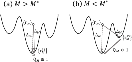
Figure 2: Sketch of the potential energy landscape showing the initial equilibrium configuration $\{{\bf r}_{\infty}\}$, and the inherent structure $\{{\bf r}_{M}^{\rm IS}\}$ obtained after swapping the diameters within each $M$ species. (a) When $M>M^{*}$, the system stays in the same basin so that $Q_{M}\simeq 1$ and $\Delta_{M}\simeq\Delta_{\infty}$. (b) When $M<M^{*}$, the system moves to another basin so that $Q_{M}\ll 1$ and $\Delta_{M}\gg\Delta_{\infty}$. $M^{*}$ is defined from the crossover between situations (a) and (b).

To determine $M^{*}$, we prepare equilibrium configurations of the original continuously polydisperse system characterized by a distribution $f(\sigma)$. We denote by $\{{\bf r}_{\infty}\}$ the original configuration, see Fig. 2. In order to characterize whether the system stays physically in the same basin or moves to another basin as a result of the swaps, we perform a quench of the system into the inherent structure (IS) Stillinger and Weber (1982). The IS corresponding to the initial configuration is denoted as $\{{\bf r}_{\infty}^{\rm IS}\}$.

We then decompose $f(\sigma)$ into $M$ species, from $M=1$ where the system is treated as an one-species system, to $M=\infty$ which describes the original system. In practice we stop at the large value $M=100$. For a given $M$ value, we systematically perform diameter swaps within each species ($m$ $\leftrightarrow$ $m$, with $m=1,\cdots,M$). More precisely, for a given configuration, we randomly pick a pair of particles within the same species and exchange their diameters. We repeat such diameter swap $N$ times so that most of the particles in the configuration experience the swap. Once the swaps have been performed, we quench the obtained configuration to its IS, which we denote by $\{{\bf r}_{M}^{\rm IS}\}$. Our goal is to monitor whether the system lands in a different basin (for $M<M^{*}$) or not (for $M>M^{*}$), as sketched in Fig. 2. To this end we monitor the following three quantities.

• The IS energy $e_{\rm IS}$ Stillinger and Weber (1982). When the system moves to another basin, $e_{\rm IS}$ should change from the value it has in the original basin.

• The overlap $Q_{M}$ between the IS configurations $\{{\bf r}_{\infty}^{\rm IS}\}$ and $\{{\bf r}_{M}^{\rm IS}\}$:

  $$Q_{M}=\frac{1}{N}\sum_{i,j}^{N}\theta(a-|{\bf r}_{Mi}^{\rm IS}-{\bf r}_{\infty j}^{\rm IS}|),$$ (17)

  where $\theta(x)$ is the Heaviside step function, and $a$ is a microscopic threshold lengthscale. By definition, $Q_{\infty}=1$, whereas we expect that $Q_{M}$ decreases from $1$ with decreasing $M$.

• The mean-squared displacement between the original equilibrium configuration $\{{\bf r}_{\infty}\}$ and the swapped IS $\{{\bf r}_{M}^{\rm IS}\}$:

  $$\Delta_{M}=\frac{1}{N}\sum_{i=1}^{N}|{\bf r}_{Mi}^{\rm IS}-{\bf r}_{\infty i}|^{2},$$ (18)

  so that $\Delta_{\infty}$ corresponds approximately to the plateau value of the mean-squared displacement reached in the physical dynamics of the original system.

If the system falls into a different basin, one expects that $Q_{M}$ will strongly decay from 1 and that $\Delta_{M}$ will increase significantly from $\Delta_{\infty}$, as shown in Fig. 2. When $M>M^{*}$, the system remains in the same basin after the swaps and the quench, showing that $Q_{\rm M}\simeq 1$ and $\Delta_{M}\simeq\Delta_{\infty}$. On the other hand, when $M<M^{*}$, the original basin is destroyed, and the system moves to another basin, showing that $Q_{\rm M}\ll 1$ and $\Delta_{M}\gg\Delta_{\infty}$. We expect that $M^{*}$ can be defined as a crossover value between these two extreme cases.

More precisely, we perform the following algorithm to determine $M^{*}$.

General Algorithm: Swap and quench protocol

• Define $M$ species by dividing the distribution $f(\sigma)$ into $M$ finite bins.

• Prepare an equilibrium configuration of the original continuous polydisperse system, $\{{\bf r}_{\infty}\}$.

• Randomly pick up a pair of particles within the same bin, and exchange their diameters. Do $N$ such exchanges.

• Quench the system and obtain $\{{\bf r}_{M}^{\rm IS}\}$.

• Repeat 1) - 4) for a large number of configurations for a wide range of $M$ values, between $M=1$ and $M=100$.

• Plot $e_{\rm IS}$, $Q_{M}$ and $\Delta_{M}$ as a function of $M$ and determine $M^{*}$ as a crossover value.

This “swap and quench” protocol is a natural way to determine $M^{*}$ which follows from the theoretical idea described in Sec. II. In this protocol, the distribution of the particle diameters $f(\sigma)$ is unaffected after defining $M$ and after the diameter swaps.

We have considered the following alternative scheme where one literally performs a discretization of the diameters into $M$ species and monitor the effect of this coarse-graining on the basin. However, we found that this coarse-graining process may affect the thermodynamic state point of the system for soft potentials. Therefore, we use this method only for hard sphere systems so that the volume fraction (and therefore the thermodynamic state point) does not change. For completeness we also present this alternative “coarse-graining and quench” protocol. Most of this procedure is as in the above “swap and quench” protocol except for item 3) which is replaced by:

• Discretize the diameters of the original system into $M$ discrete species keeping the global volume fraction constant.

We have checked that the two protocols give essentially the same results for hard spheres, as shown below. We mention the coarse-graining procedure as a way to trigger the imagination of future researchers towards the implementation of numerical procedures alternative to ours.

It is important to realize that the discretization of the particle size distribution in step 1) of the algorithm is not uniquely defined. For the particular case under study, it is physically meaningful to choose equal intervals $\Delta\sigma=(\sigma_{\rm max}-\sigma_{\rm min})/M$, such that each discretized species occupies the same fraction of the total volume, but one can imagine that non-uniform intervals could be better choices for more complicated particle size distributions. We have not addressed this point in detail, but it would deserve further study.

III.2 Details of our models and simulations

We perform molecular simulations for several pair potentials in three dimensions Allen and Tildesley (1989), studying a total of five different numerical models.

We use a continuous size polydispersity, where the particle diameter $\sigma$ of each particle is randomly drawn from the following particle size distribution: $f(\sigma)=A\sigma^{-3}$, for $\sigma\in[\sigma_{\rm min},\sigma_{\rm max}]$, where $A$ is a normalization constant. We define the size polydispersity as $\delta=\sqrt{\overline{\sigma^{2}}-\overline{\sigma}^{2}}/\overline{\sigma}$, where $\overline{\cdots}=\int\mathrm{d}\sigma f(\sigma)(\cdots)$. We mainly use $\delta=0.23$, choosing $\sigma_{\rm min}/\sigma_{\rm max}=0.4492$ when studying different pair potentials, as shown in Fig. 1. To investigate the effect of $\delta$ we also study the case $\delta=0.176$ choosing $\sigma_{\rm min}/\sigma_{\rm max}=0.543$ for the hard sphere potential. We use $\overline{\sigma}$ as the unit length. We simulate systems composed of $N$ particles in a cubic cell of volume $V$ with periodic boundary conditions Allen and Tildesley (1989). The canonical ensemble is used throughout this paper.

We use the following pairwise potential for the soft sphere models,

$$v_{ij}(r) = v_{0}\left(\frac{\sigma_{ij}}{r}\right)^{n}+c_{0}+c_{1}\left(\frac{r}{\sigma_{ij}}\right)^{2}+c_{2}\left(\frac{r}{\sigma_{ij}}\right)^{4},$$ (19)

$$\sigma_{ij} = \frac{(\sigma_{i}+\sigma_{j})}{2}(1-\eta|\sigma_{i}-\sigma_{j}|),$$ (20)

where $v_{0}$ is the unit of energy, and $\eta$ quantifies the degree of non-additivity of the particle diameters. Non-additivity is introduced for convenience, as it prevents more efficiently crystallization and thus it enhances glass-forming ability of the numerical models. The constants, $c_{0}$, $c_{1}$ and $c_{2}$, are chosen so that the first and second derivatives of $v_{ij}(r)$ become zero at the cut-off $r_{\rm cut}=1.25\sigma_{ij}$. We employ the additive and non-additive soft sphere models using the parameters $n=18$, $\eta=0$ (additive) and $n=12$, $\eta=0.2$ (non-additive), respectively. We set the number density $\rho=N/V=1.0$ with $N=1500$ for the soft sphere models.

We also use hard sphere models in three dimensions, where the pair interaction is zero for non-overlapping particles, and infinite otherwise. We employ both additive ($\eta=0$) and non-additive ($\eta=0.2$) systems of hard spheres, using Eq. (20). Also, we analyze an additive hard sphere system with $\delta=0.176$. We use $N=1000$ for the additive hard sphere systems and $N=300$ for the non-additive systems. We have also performed simulations using $N=300$ and $8000$ for additive hard spheres with $\delta=0.23$ and find that there is no significant finite size effects in our results. The hard sphere simulations are presented as a function of the reduced pressure $Z=P/(\rho k_{B}T)$, where $P$ is the measured pressure, and $k_{B}T$ is set to unity.

The initial equilibrium configurations for the protocols described in Sec. III.1 need to be deeply supercooled either at very low temperatures (for soft sphere potentials) or high pressures (for hard spheres). To this end, we employ a swap Monte-Carlo (MC) method for all models. This approach is a very efficient thermalization algorithm which enables us to easily reach sufficiently supercooled equilibrium regimes. The details of these efficient simulations are provided in Ref. Ninarello, Berthier, and Coslovich, 2016 for the soft sphere models and Ref. Berthier et al., 2016b for the hard sphere models.

Finally to perform the quench of the system into its inherent structure, we use a conjugate gradient method Nocedal and Wright (2006) for the soft sphere systems. To realize the quench for the hard sphere systems, we perform non-equilibrium compressions up to the jamming volume fraction $\phi_{J}$ Stillinger and Weber (1985); Chaudhuri, Berthier, and Sastry (2010); Ozawa et al. (2012). Specifically we employ the jamming algorithm described in Ref. Xu, Blawzdziewicz, and O’Hern, 2005; Desmond and Weeks, 2009 to perform these nonequilibrium compressions.

IV Numerical validation of the method

IV.1 Practical determination of $M^{*}$

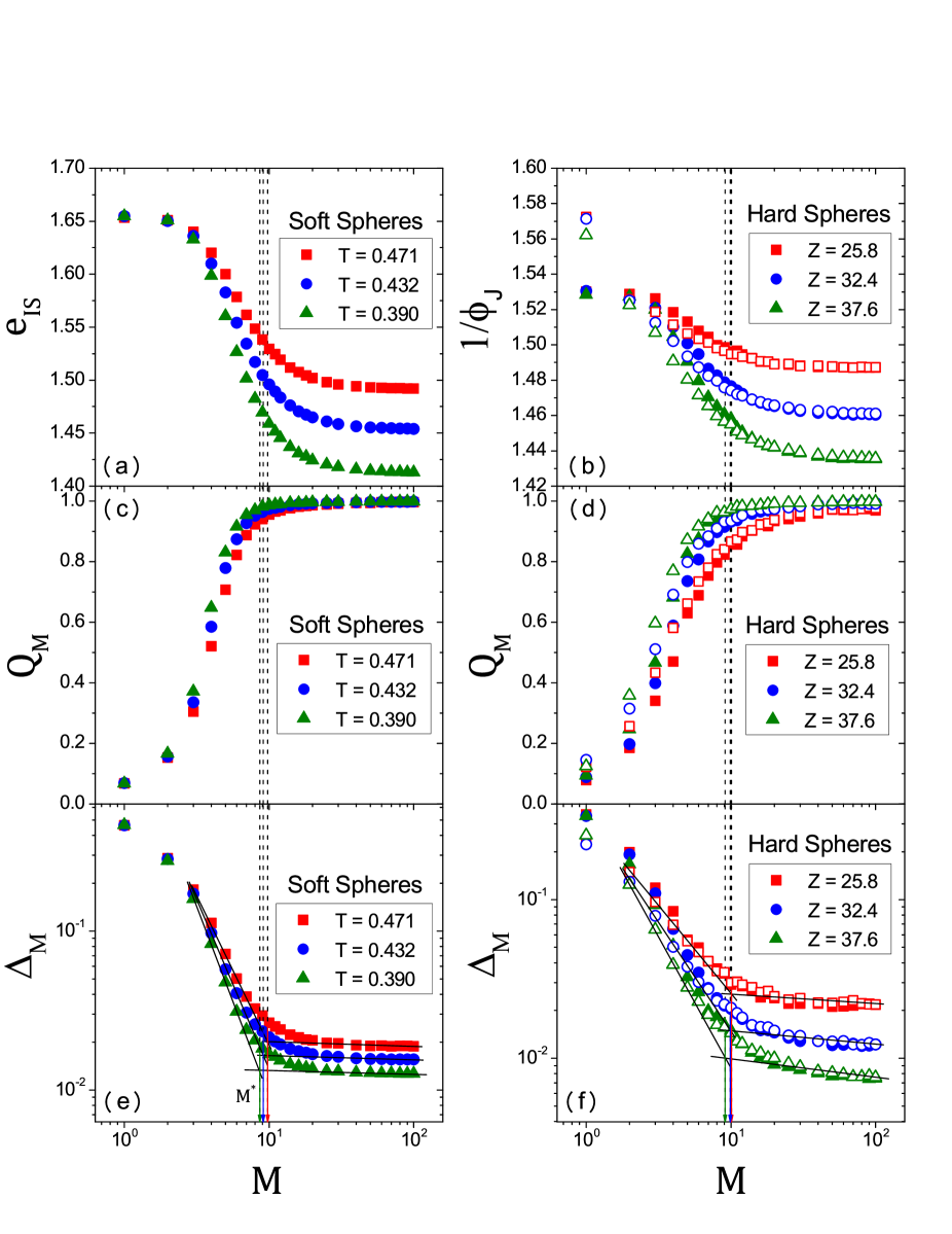
Figure 3: (a, b) Inherent structure energy $e_{\rm IS}$ and volume $1/\phi_{\rm J}$. (c, d) Overlap $Q_{M}$. (e, f) Mean-squared displacements $\Delta_{M}$. The results are for additive soft spheres (left panels) and additive hard spheres (right panels) with $\delta=0.23$. The vertical dashed lines represents the $M^{*}$ values determined by the intersection of the two power law regimes in the mean-squared displacements in (e, f). In addition to the “swap and quench” protocol with closed symbols, results for the “coarse-graining and quench” protocol are also shown for hard spheres using open symbols.

We now present our numerical results. In Fig. 3, we show the evolution of the inherent structure energy $e_{\rm IS}$ (or the volume at jamming $1/\phi_{\rm J}$ for hard spheres), of the overlap $Q_{M}$, and of the mean-squared displacement $\Delta_{M}$ as a function of $M$ for both a soft sphere model and a hard sphere model. All the other models we have studied behave similarly. To compute $Q_{M}$, we set $a=0.23$ for all systems. This value was used earlier to characterize metastable states and the phase transitions among them Berthier and Jack (2015); Berthier et al. (2016a).

The results of the additive soft sphere model with $\delta=0.23$ are presented in the left panels of Fig. 3. At large $M$, we observe nearly constant values of $e_{\rm IS}(M)\simeq e_{\rm IS}(M\to\infty)$, $Q_{M}\simeq 1$, and $\Delta_{M}\simeq\Delta_{\infty}$, which means that the swap of the diameters within each $M$ species marginally affects the system. Thus, after the diameter swaps, the system essentially remains in the original basin. However, with decreasing $M$, all observables start to deviate significantly from their large-$M$ limits. As $M$ decreases, we find that $e_{\rm IS}$ increases, $Q_{M}\to 0$, and $\Delta_{M}$ increases rapidly. These observations indicate that at smaller $M$, the effect of the swap is so strong that the original basin is destroyed, and the system moves to another basin.

It is clear from these figures that a clear crossover occurs between large and small $M$ behaviors, which we wish to use to determine $M^{*}$ quantitatively. However, because $M^{*}$ describes a smooth crossover, it cannot be defined unambiguously. From a careful analysis of all these observables for all models, we conclude that $\Delta_{M}$ is the best quantity to determine $M^{*}$, because it appears as the most sensitive measure of the change of basin. As shown in Fig. 3(e), we determine $M^{*}$ as the intersection of two power law regimes obeyed at large and small values. For the soft sphere model in Fig. 3(e), we obtain $M^{*}\simeq 8.5-10$ with a weak temperature dependence. These values of $M^{*}$ are also reported in the figures for $e_{\rm IS}$ and $Q_{M}$ by the vertical dashed lines. It is clear that they identify also very well the crossover behavior observed in these two observables, even though their crossover behavior is less sharply defined.

In the right panels of Fig. 3, we show the results for the additive hard sphere system with $\delta=0.23$. We observe a behavior which is qualitatively similar to the soft sphere model, and we determine that $M^{*}\simeq 9-10$ using again the $M$-dependence of $\Delta_{M}$ in Fig. 3(f).

In addition, for hard spheres we can also compare these results obtained with the “swap and quench” protocol, to the “coarse graining and quench” protocol. The results for the latter procedure are shown with open symbols in Fig. 3. The excellent agreement between the two sets of results is evident and this second protocol thus yields the same values of $M^{*}$.

IV.2 Results for $M^{*}$ and $S_{\rm mix}^{*}$

We have repeated the measurements shown in Fig. 3 for the five different numerical models considered in this work. For each model, we obtain $M^{*}$ for a broad range of deeply supercooled state points. Finally, using the simple procedure shown in Fig. 1(b), we convert these $M^{*}$-values into an estimate of the effective mixing entropy $S_{\rm mix}^{*}$, which we could then use to determine the configurational entropy of these continuously polydisperse systems.

Figure 4: Evolution of $M^{*}$ for two soft sphere systems (a) and three hard sphere systems (b). (c, d) show the corresponding effective mixing entropy $S_{\rm mix}^{*}$. The horizontal axes are normalized by the mode-coupling transition points, $T_{c}$ and $Z_{c}$ to facilitate the comparison between the different models. In addition to the “swap and quench” protocol (closed symbols), results for the “coarse-graining and quench” protocol (open symbols) are also shown for hard spheres.

We compile all our results for $M^{*}$ and $S_{\rm mix}^{*}$ as a function of $1/T$ (for soft potentials) and $Z$ (for hard spheres) in Fig. 4. The temperature and pressure scales are normalized by the mode-coupling transition points, $T_{c}$ and $Z_{c}$, in order to facilitate the comparison between different glass-formers. As usual, $T_{c}$ and $Z_{c}$ are determined by a power-law fit of the relaxation times Ninarello, Berthier, and Coslovich (2016); Berthier et al. (2016b). Notice that all studied state points correspond to fluid states thermalized well beyond the mode-coupling crossover.

We find that $M^{*}$ and hence $S_{\rm mix}^{*}$ slightly decrease with decreasing $T$ or increasing $Z$, and this effect seems more pronounced for the soft sphere models. Physically, this reflects the fact that the basin becomes more robust against particle exchanges at lower $T$ or higher $Z$. This variation is a direct confirmation that $M^{*}$ represents a non-trivial characterization of the glassy states, which needs to be numerically determined independently for each state point, at least in principle.

In practice however, it is a very good approximation to consider that the effective mixing entropy $S_{\rm mix}^{*}$ of hard spheres is essentially constant in the deeply supercooled fluid. In addition, in the hard sphere systems the two distinct protocols introduced above give quantitatively consistent values, especially at large $Z$, which again confirms the robustness of our numerical approach.

Remarkably, the value of $M^{*}$ for the additive system with $\delta=0.176$ is about $20\%$ smaller than that of the system with $\delta=0.23$, which may be rationalized by the corresponding relative reduction of the polydispersity (of about $\approx 23~{}\%$). Thus, our results appear in agreement with the physical expectation that $(M^{*}-1)$ should be proportional to the polydispersity $\delta$. We would need more data at different polydispersities to confirm this result quantitatively. However, a rough extrapolation of these $M^{*}$ values towards smaller polydispersity values, suggests that $M^{*}\simeq 4-5$ for $\delta=0.10$ and $M^{*}\simeq 2-3$ for $\delta\simeq 0.05$, whereas smaller polydispersities should essentially be treated as mono-component systems. We can also translate these findings into a critical value $(1+\epsilon^{*})\simeq 1.1$ for the size ratio below which two particles should be treated as having the same size.

Finally, we note that for the relatively polydisperse systems that we study, the effective mixing entropies are of order $S_{\rm mix}^{*}/N\simeq 2.0$. Given that the configurational entropy is typically of order $S_{\rm conf}/N\simeq 1.0$ near the onset of slow dynamics Sciortino, Kob, and Tartaglia (1999); Angelani and Foffi (2007), we conclude that an accurate determination of the mixing entropy is indeed crucial to properly estimate the configurational entropy.

V Discussion and perspectives

In this paper, we discussed the problems of the conceptual definition and of the practical measurement of the configurational entropy $S_{\rm conf}$ in glass-forming models characterized by a polydisperse size distribution, inspired by the physics of colloidal materials. We first noticed that standard approaches to estimate the configurational entropy fail in the case of a continuous polydispersity, providing either an infinite or an incorrect estimate of $S_{\rm conf}$ depending on an arbitrary choice made regarding the mixing entropy contribution. We then proposed a simple method to compute a finite and physically-meaningful configurational entropy $S_{\rm conf}$ in continuously polydisperse systems which relies on a treatment of the original system as an effective $M^{*}$-component system, where $M^{*}$ is finite and has to be measured directly at each state point. Finally, we performed numerical simulations of five different glass-forming models and showed that our approach provides meaningful results in all cases.

The key idea leading to a finite configurational entropy for polydisperse systems is the distinction between configurations (or their corresponding inherent structures) in the phase space volume and states defined as free energy minima. While the configurational entropy should be interpreted or quantified as the (logarithm of the) number of states, the inherent structure approaches instead quantify the (logarithm of the) number of inherent structures associated to configurations. While this may represent a correct approximation in some specific instances, the confusion between the two concepts has important consequences for polydisperse mixtures, as the number of configurations (and hence of inherent structures) diverges, while the number of states does not. This conceptual distinction has been discussed at length in the literature Biroli and Monasson (2000); Berthier and Biroli (2011), as the confusion between states and configurations is at the root of several arguments suggesting the impossibility of an ideal glass transition Stillinger (1988); Donev, Stillinger, and Torquato (2007); Eckmann and Procaccia (2008). Therefore, the case of polydisperse materials is one more instance where this confusion may lead to paradoxical results.

We mentioned in the introduction the recently-proposed alternative method to compute the configurational entropy, based on the Franz-Parisi construction, which relies on estimating the free energy difference between the fluid and glass states Franz and Parisi (1997); Berthier and Coslovich (2014). This method does not suffer from a possible divergence in the mixing entropy, because it does not involve estimating the entropy of the fluid and glass states separately.

In fact, the conceptual difference between the standard approach ($S_{\rm conf}=S_{\rm tot}-S_{\rm vib}$) and the Franz-Parisi construction is easy to grasp from their practical implementations. Both approaches rely on performing thermodynamic measurements on systems constrained to evolve ‘near’ a given reference configuration. When using the Frenkel-Ladd method in the standard approach Coluzzi et al. (1999); Sastry (2000); Angelani and Foffi (2007), the constraint is a set of harmonic springs connecting each particle to reside close to its position in the reference configuration. Instead, in the Franz-Parisi approach, one constrains the collective density profile to reside close to the one of the reference configuration. For the particular case of polydisperse systems, the collective nature of this constraint allows particle permutations in the glass state which are then automatically taken into account with their correct equilibrium weight. Note that the standard definition of the overlap used in this approach does not take into account the particle diameters. One could imagine generalizing this definition to prevent particle permutations between particles with very different diameters, which would result in a different estimate of the configurational entropy, suggesting that a more careful study of the effect of size polydispersity within the Franz-Parisi approach would be very valuable too. In order to use the standard approach we have shown that it is necessary to correct for the (incorrect) ‘self’ nature of the constraint by estimating separately an effective mixing entropy contribution, and we have proposed a simple method to do so.

Because both methods provide distinct conceptual estimates of the configurational entropy, there is no reason why they should yield identical absolute values of $S_{\rm conf}$ in the supercooled liquid regime. In the presence of a genuine ideal glass transition, however, both methods should yield consistent results for its location. In Ref. Berthier et al., 2016a, we have computed the volume fraction dependence of the absolute value of $S_{\rm conf}$ for the additive hard sphere system with $\delta=0.23$ studied in the present work, using both the present approach and the Franz-Parisi construction. The results show that the agreement between the two methods is good Berthier et al. (2016a).

Note that in experiment, the configurational entropy is obtained by integration of the heat capacity difference between the fluid and crystal states Richert and Angell (1998), where it is assumed that the vibrational (or glass) entropy is well approximated by the entropy of the crystal Yamamuro et al. (1998); Angell and Borick (2002). The reference point which sets the absolute value of the configurational entropy is given by the entropy of fusion. Therefore, traditional experimental measurements of the configurational entropy do not suffer from the problem of the mixing entropy, because the experimental procedure does not require estimating the absolute entropy of any state point. This experimental procedure could be applied to systems with continuous polydispersity, because the experimental definition of the configurational entropy simply requires a thermodynamic integration along an equilibrium path. Of course, the drawback of this procedure is that it is unclear whether the experimental protocol truly reflects the theoretical definition of a configurational entropy related to the number of free energy minima. Therefore, for theoretical purposes we do not wish to follow the experimental procedure to solve the issue raised by polydispersity. Similarly, the experimental path cannot be followed in computer simulations where the properties of the equilibrium crystal are usually unknown, and thermodynamic integration across the nonequilibrium glass transition would yield incorrect results. Therefore, it is numerically necessary to carefully estimate the mixing entropy.

In this paper, we defined $M$ discretized species by dividing the distribution $f(\sigma)$ into equal intervals $\Delta\sigma=(\sigma_{\rm max}-\sigma_{\rm min})/M$, such that each species occupies the same fraction of the total volume for the specific distribution shown in Fig. 1(a). However, one can expect that non-uniform intervals $\Delta\sigma_{m}$, could be applied to general distributions $f(\sigma)$. Whereas non-uniform intervals might change the value of $M^{*}$ and functional form of $S_{\rm mix}^{(M)}$, we would expect that the resulting $S_{\rm mix}^{*}$ does not depend on the binning process as long as physically reasonable discretizations producing relatively small $M^{*}$ values are applied. Finding such reasonable non-uniform intervals for general distributions $f(\sigma)$ is an important topic for future studies.

Our numerical protocol, which transforms a continuously polydisperse system into an $M^{*}$-component system, is also useful for more general theoretical investigations, since finite mixtures are theoretically more tractable than continuously polydisperse systems Coluzzi et al. (1999); Biazzo et al. (2009); Weysser et al. (2010). For example, theoretical computations of the thermodynamics of the glass phase in (finite and discrete) multi-components mixtures Coluzzi et al. (1999); Biazzo et al. (2009) could more easily be applied once $M^{*}$ is numerically determined. In the same vein, in Ref. Weysser et al., 2010, the multi-components extension of the mode coupling theory is compared with simulations of a continuous polydisperse system with $\delta=5.8\%$. The theory seems to describe well simulation results regarding glassy dynamical behaviors when $M\geq 3$, which is in good agreement with the estimate obtained in our work assuming that $(M^{*}-1)$ is proportional to $\delta$. Our work in fact paves the way for an analytical treatment of the glass thermodynamics of continuously polydisperse particle systems. Another interesting theoretical goal would be the analytical derivation of the critical size ratio $(1+\epsilon^{*})$ separating the regime where particles should be treated as identical or as distinct, as this would allow a fully analytical treatment of polydisperse materials. Recently, a starting point for this direction has been developed Ikeda, Miyazaki, and Ikeda (2016). When applied to hard spheres, predictions could then be made regarding the influence of the polydispersity on the jamming transition, which is another topic of interest.