On dust-gas gravitational instabilities in protoplanetary discs

Abstract

In protoplanetary disks the aerodynamical friction between particles and gas induces a variety of instabilities that facilitate planet formation. Of these we examine the so called ‘secular gravitational instability’ (SGI) in the two-fluid approximation, deriving analytical expressions for its stability criteria and growth rates. Concurrently, we present a physical explanation of the instability that shows how it manifests upon an intermediate range of lengthscales exhibiting geostrophic balance in the gas component. In contrast to a single-fluid treatment, the SGI is quenched within a critical disk radius, as large as 10 AU and 30 AU for cm and mm sized particles respectively, although establishing robust estimates is hampered by uncertainties in the parameters (especially the strength of turbulence) and deficiencies in the razor-thin disk model we employ. It is unlikely, however, that the SGI is relevant for well-coupled dust. We conclude by applying these results to the question of planetesimal formation and the provenance of large-scale dust rings.

1 Introduction

The assembly of planets is a complex and multi-faceted phenomenon that spans a gulf of some 12 orders of magnitude in length: from micron-sized dust to $10^{3}$ km planetary cores. It draws on an equally wide range of physical processes: collisions, dust-gas aerodynamics, gravitational collapse, instabilities, and disk structures (e.g. vortices, dust traps), to name but a few (Papaloizou & Terquem 2006, Chiang & Youdin 2010, Armitage 2010). While it is relatively straightforward to grow cm sized particles from micron sizes, further growth is potentially halted by a number of ‘barriers’ (bouncing, fragmentation, radial-drift; Johansen et al. 2014). Statistically a small number of ‘lucky’ aggregates may hurdle these, but certain collective instabilities can aid aggregation through this difficult size range. These include classical gravitational instability (GI; Safronov 1969, Ward & Goldreich 1973), streaming instability (Youdin & Goodman 2005), and the secular gravitational instability (SGI; Ward 2000, Youdin 2005). It is to the last instability that this paper is devoted.

One of the most attractive features of the single-fluid SGI is that its onset is unconditional; it should always be present. Unlike classical GI, which requires the Toomre parameter to be less than one, a single fluid analysis presents no analogous restriction: the SGI works no matter how thin or thick the particle sub-disk (Youdin 2005). The instability attacks longer scales preferentially, which ordinarily would be stabilised by the Coriolis force; but particles can shed (or gain) angular momentum via areodynamical drag, and hence are not obliged to undergo stabilising epicycles. As a consequence, rings that are radially drifting towards each other continue to do so unimpeded, and the instability can proceed. On small radial scales the SGI is suppressed by dust pressure or gas turbulence, and in fact, for well-coupled dust, turbulence decreases growth rates to potentially insignificant levels (Shariff & Cuzzi 2011, Youdin 2011). Marginally coupled particles, however, could still be subject to respectable SGI growth rates at certain radii.

The SGI has been thoroughly explored in single fluid models, which are applicable when the dust to gas density ratio is tiny (e.g. Ward 2000, Youdin 2005, Shariff & Cuzzi 2011, Youdin 2011, Michikoshi et al. 2012). These models assume that the angular momentum bestowed onto, or removed from, the gas disk is negligible. On sufficiently long scales, however, both sides of this momentum transaction must be included and the gas dynamics explicitly calculated. An instability criterion then appears: in a two-fluid model the onset of SGI is no longer unconditional. Recently, Takahashi & Inutsuka (2014, hereafter TI) made a start on this problem (see also Shadmehri 2016 and Takahashi & Inutsuka 2016), but there is still much to be established. Putting aside the issue of growth rates, an especially important question is: at what radii and for what particle sizes should we expect SGI to exist at all?

The first aim of this paper is to derive clean stability criteria for the SGI. In the limits of strongly-coupled and weakly-coupled particles these can be formulated analytically and involve a variety of parameters, including the gas’s Toomre parameter and the dust-to-gas density ratio. Because they bypass the SGI’s full 6th order dispersion relation, these criteria make it relatively easy to assess its prevalence.

The criteria also motivate a straightforward physical picture of instability in a two-fluid system. In order for the instability to work, there must exist an intermediate range of lengthscales gas upon which (a) dust pressure or turbulent mass diffusion is subdominant, and (b) the gas is prevented from executing epicycles, despite its angular momentum transactions with the dust. Going to lengthscales longer than the dust pressure (or diffusion) scale takes care of the first restriction. But the second can only be satisfied if geostrophic balance holds in the gas fluid, and so we must simultaneously find shortish scales upon which gas pressure is dominant. The existence or not of this intermediate range furnishes us with the stability criterion.

The formalism is applied to realistic disk models, where we find that it is unlikely that well-coupled dust is unstable to the SGI at any radius, unless the background turbulence is especially weak. Marginally coupled particles, however, can achieve appreciable growth rates in certain circumstances, emphasising that the SGI could help aggregation of solids of cm size. We conclude, however, that SGI is probably unrelated to the dust rings recently observed by ALMA (Brogan et al. 2015).

The paper will be organised in the following way. First, in Section 2, we present the two-fluid razor-thin disk model that we employ, alongside a critical discussion of its shortcomings. The main parameters of the analysis will also be defined. In Section 3 we revisit the single-fluid model to fix some ideas and to provide context for the subsequent analysis, while in Section 4 we briefly treat a simple two-fluid system where the gas is regarded as incompressible. The main results of the paper are in Section 5, in which we derive analytic stability criteria in relevant limits that are then applied to realistic disk models in Section 6. We draw our conclusions in Section 7, where we discuss the relevance of the SGI in planet and structure formation in protostellar disks.

2 Preliminaries

2.1 Modelling issues

The classical GI and secular GI have primarily been explored with 1D models of a vertically averaged or razor-thin disk. Recent notable exceptions are Mamatsashvili & Rice (2010) and Lin (2014), who also capture vertical convection and the magnetorotational instability respectively. A 1D model certainly eases the analysis and it should be a reasonable approximation for unstable modes whose radial wavelength is much greater than the disk thickness; because the classical GI has minimal vertical structure (being essentially an f-mode in this limit; Ogilvie 1998), it is also likely that the SGI depends on $z$ only weakly. For wavelengths closer to the scale height, a somewhat ad hoc correction may be included (e.g. Shu 1984), which generally works against instability on these shorter lengthscales.

In a two-fluid model, however, the razor-thin assumption is complicated by the fact that the particle fluid and the gas fluid possess different thicknesses, and the former can be significantly shorter than the latter. This is a problem for the SGI because the fastest lengthscales are not far from the particle scale height (Youdin 2005), and hence of order or less than the gas scale height. As a consequence, the approximation of a razor-thin disk is not strictly applicable, at least in the description of the gas. In a single fluid model this issue does not crop up because it is assumed that the gas fluid is unperturbed by whatever the dust is doing; but in a two fluid model this is not the case. It may be that the gas perturbations associated with the SGI are sufficiently small that the disk’s vertical structure plays little role. But only calculations in vertically stratified shearing boxes can decide on this point.

A second issue is the correct coupling between the two fluids. In a real system, with different gas and dust scale heights, the drag acceleration will be a function of vertical height $z$. Moreover, the entire column of gas will not exert drag on the dust if the dust subdisk is much thinner. For consistency, the gas external to the dust disk should be excluded from a two-fluid razor-thin treatment, with the weighting of the drag force in the momentum equation adjusted appropriately to account for the smaller surface density of the gas subdisk. Because most of the mass in both disks is near the midplane, this problem may not invalidate the main qualitative results. It should, however, be kept in mind.

A third issue concerns turbulence in the gas, its effects, and how to mathematically describe it. The gas is likely undergoing disordered motions at some (perhaps all) radii, though the underlying physics may differ between different regions (Turner et al. 2014). The disk may also support turbulence because of the settling of the dust to the midplane, and ensuing vertical Kelvin-Helmholtz instability (Cuzzi et al. 1993). The consequences of turbulence on particles are several. Agitation of the solids produces enhanced velocity dispersions, over and above that arising from particle collisions (Goldreich & Tremaine 1978), and thus an appreciable particle pressure that will oppose vertical settling. The precise ‘equation of state’ this pressure obeys, however, is difficult to establish. In addition, the random motions induced in the dust can potentially smooth away inhomogeneities in the dust density, and thus lead to diffusion in the continuity equation directly (Youdin 2011, Shariff & Cuzzi 2011, Takahashi & Inutsuka 2012). The efficiency of this diffusion is pretty much unconstrained and obviously requires numerical exploration; for instance, the vertical Kelvin-Helmholtz instability will mix particles effectively in the vertical direction but not necessarily in the horizontal. Finally, turbulence will transport momentum, though this effect (being a straightforward mild damping) we do not include in this paper (see TI for its treatment).

The effects of turbulence on the dust have been mathematically modelled via mean-field theories, and Langevin and Fokker-Planck equations (e.g. Schräpler & Henning 2004, Carballido et al. 2006, Youdin & Lithwick 2007). Given a Kolmogorov spectrum of isotropic homogeneous turbulent motions, Youdin & Lithwick (2007) derive convenient expressions for the dust velocity dispersion and the turbulent diffusivity of particle mass, in terms of the stopping time and a turbulent efficiency parameter (described below). Such a calculation, of course, must assume that the turbulent flux of particles behaves as a Fickian diffusion — which it need not, especially on scales close to the largest ‘eddy’. Other complications could arise from the flux’s finite relaxation time and possible anti-diffusive behaviour (especially on small scales, e.g. Frisch 1995 Davidson 2000, Cuzzi et al. 2001).

Our purpose in this paper is not to improve on any of these issues, but it is important to flag them at this point. We persist with the simple models previously employed (e.g. TI, Shadmehri 2016), mainly because they can fix ideas and establish clear results, and presumably give approximately correct predictions. Future work, however, should involve vertically stratified models along the lines of Mamatsashvili & Rice (2010) and Lin (2014).

2.2 Parameters

As will become clear by Section 5, the two-fluid secular GI is governed by a large number of parameters; it is hence convenient to define them all in one place. The first key parameter is the dust-to-gas mass ratio, denoted by $\delta$ and defined via

$$\delta=\frac{\sigma_{a}}{\sigma_{g}},$$ (1)

where $\sigma_{a}$ is the background surface density of the dust with size $a$, and $\sigma_{g}$ is the surface density of the gas located within the dust subdisk (see earlier). Thus $\delta$ is a function of $a$. Because the SGI is size-selective it is necessary to distinguish between particles of different sizes, and thus to use separate surface densities for each subspecies. To ease the analysis in this paper we examine each dust species separately, though in reality different species will weakly couple via the gas phase. See Shadmehri (2016) for an attack on a system of interacting gas and two species of particle.

Generally, $\sigma_{a}$ is a small fraction of the total solid surface density. In fact, the surface density of mm and cm sized particles can be significantly less than 1% of the total (e.g. Brauer et al. 2008, Windmark et al. 2012a, 2012b), though this figure varies greatly with age and as different physical processes are included or neglected (sticking, bouncing, fragmentation, and mass tranfer, for instance; Garaud et al. 2013). Note that $\sigma_{g}$ will also be less than the total gas density, as it only includes gas situated amongst the dust subdisk. This decrease can be quantified by a factor $\sim H_{g}/H$, where $H_{g}$ and $H$ are the scale thicknesses of the gas and dust respectively. We may then write

$$\delta\approx 0.01\,\left(\frac{\sigma_{a}}{\sigma_{\text{tot}}}\right)\left(\frac{H_{g}}{H}\right),$$ (2)

where $\sigma_{\text{tot}}$ is the total dust surface density (including all species), and we have assumed that the ratio of total dust to total gas density takes the standard value 0.01 (Chiang & Youdin 2010). Given the large uncertainties in the second and third factors in Eq. (2) (small and large respectively), we simply set $\delta=0.01$ for most calculations.

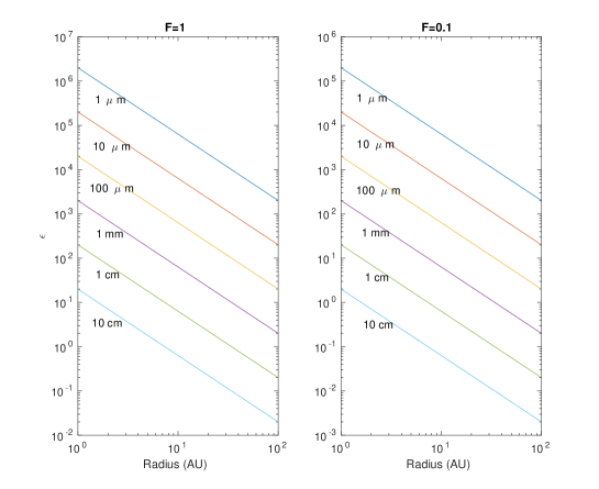
Figure 1: Inverse Stokes number $\epsilon$ as a function of radius for different particle sizes and two different minimum mass solar nebulae models, as calculated from Youdin (2011) but only using the Epstein drag regime. The $F=1$ case corresponds to a nebula with a gas surface density of 2000 gcm^-2 at 1 AU, while $F=0.1$ corresponds to 200 gcm^-2. See Eq. 55.

The second key parameter is the inverse Stokes number, which we denote by $\epsilon$ and define through

$$\epsilon=\frac{1}{\tau_{s}\Omega},$$ (3)

where $\tau_{s}$ is the stopping time of the particles, and $\Omega$ is the local orbital frequency. Large values of $\epsilon$ correspond, thus, to strongly coupled particles, and smaller values to weakly coupled particles. The exact value of $\epsilon$ depends on particle size, naturally, but also on radial location (e.g. Chiang & Youdin 2010). Fig. 1 gives $\epsilon$ profiles for two different minimum mass solar nebulae (MMSN) models. See Section 6 for more details.

The third parameter is the ratio of dust and gas velocity dispersions, defined through

$$\eta=\frac{c^{2}}{c_{g}^{2}},$$ (4)

where $c$ and $c_{g}$ denote the velocity dispersion of the dust and gas respectively. To a first approximation, the dust random velocities are controlled by ‘kicks’ delivered by the gas turbulence, rather than inter-particle collisions (Youdin & Lithwick 2007). Thus it is possible to relate $\eta$ to properties of the turbulence, and we do so below. Collisional agitation becomes important for larger particles $\gtrsim$ cm, and thus the $\eta$ we use in this paper may be an underestimate for these sizes.

The fourth parameter is the Toomre $Q$ of the dust, which describes the onset of classical GI. It is given by

$$Q=\frac{c\Omega}{\pi G\sigma},$$ (5)

where $G$ is the gravitation constant and for notational convenience we have dropped the subscript ‘$a$’ from the surface density. An analogous expression can be defined for the gas, which we denote by $Q_{g}$. The two Toomre parameters can be related via the following identity: $Q_{g}=(\delta/\sqrt{\eta})Q$.

Finally, the turbulent diffusion of solid particles can be quantified via the mass diffusivity $D$, and the diffusion of gas by the analogous $D_{g}$. As in Youdin (2011), we replace these by the dimensionless parameters $\alpha$ and $\alpha_{g}$, via $D=\alpha c_{g}^{2}/\Omega$ and $D_{g}=\alpha_{g}c^{2}_{g}/\Omega$, with these related via

$$\alpha=\frac{\epsilon^{2}+\epsilon+4}{(\epsilon+\epsilon^{-1})^{2}}\alpha_{g},$$ (6)

(Youdin & Lithwick 2007, Youdin 2011). The dust’s velocity dispersion (if excited by turbulence) can also be expressed in terms of $\alpha_{g}$ and we find

$$\eta=\frac{\epsilon^{3}+2\epsilon+5/4}{\epsilon(\epsilon+\epsilon^{-1})^{2}}\alpha_{g}.$$ (7)

Thus $\alpha_{g}$ governs both $D$ and $\eta$. Unfortunately, an estimate of its magnitude is one of the great uncertainties in the theory, though it is likely to be smaller (and possible much smaller) than the analogous dimensionless coefficient associated with angular momentum transport in the gas ($10^{-3}-10^{-2}$ in a protoplanetary disk). For instance, if transport is controlled by magnetocentrifugal winds or strong zonal magnetic fields then the bulk of the disk could even be laminar (e.g. Lesur et al. 2014, Bai 2014). Having said that, vertical settling should always lead to disordered motions and some degree of radial diffusion. Putting these considerations aside, it is clear that strongly coupled particles ($\epsilon\gg 1$) have $\alpha\sim\alpha_{g}$ and $\eta\sim\alpha_{g}$; whereas weakly coupled particles ($\epsilon\ll 1$) are diffused less effectively $\alpha\sim\epsilon^{2}\alpha_{g}$ and are far ‘colder’, $\eta\sim\epsilon\alpha_{g}$.

3 A single fluid model

Though the single fluid analysis of the SGI is well-trodden territory we include it here for completeness and because it helps fix useful ideas that appear later. One especially important theme that crops up is geostrophic balance and the purely azimuthal ‘zonal’ flows that ensue.

3.1 Governing equations

As we are interested in relatively short radial scales it is convenient to employ the shearing sheet model (Goldreich & Lynden-Bell 1965), whereby a small portion of disk, centred upon a fixed radius $R_{0}$, is represented by a Cartesian box. In a corotating frame centred on the box, $x$ and $y$ denote the local radial and azimuthal coordinates, while $\Omega$ is the orbital frequency at $R_{0}$. The disk is assumed to be razor thin, so that the dust volumetric density is $\sigma(x,y)\delta(z)$, where $\sigma$ is the dust surface density and $\delta(z)$ the Dirac delta function (not the dust-to-gas mass ratio).

The equations governing the evolution of the dust fluid are given by the continuity, momentum, and Poisson equations:

$$\partial_{t}\sigma+\mathbf{u}\cdot\nabla\sigma=-\sigma\nabla\cdot\mathbf{u}+D\partial_{x}^{2}\sigma,$$ (8)

$$\partial_{t}\mathbf{u}+\mathbf{u}\cdot\nabla\mathbf{u}=-\nabla\Phi_{t}-\nabla\Phi_{\text{sg}}-\nabla P$$

$$\hskip 85.35826pt-\epsilon\Omega(\mathbf{u}-\mathbf{U})-2\Omega\mathbf{e}_{z}\times\mathbf{u},$$ (9)

$$\nabla^{2}\Phi_{\text{sg}}=4\pi G\sigma\,\delta(z),$$ (10)

where $\sigma$, $\mathbf{u}$, and $P$ denote the dust surface density, velocity, and pressure. Again we have dropped the subscript ‘$a$’ from the surface density; it is understood from here onwards that $\sigma$ refers to the surface density of particles of size $a$. The potentials associated with the dust self-gravity and tide are $\Phi_{\text{sg}}$ and $\Phi_{t}=-(3/2)\Omega^{2}x^{2}$ respectively. The gas velocity is given by $\mathbf{U}$, and it interacts with the dust via a drag term whose strength is quantified by the inverse Stokes number $\epsilon$.

In this section it is assumed that there is no appreciable backreaction of the dust on the gas motion. Moreover, we neglect the effect of any radial pressure gradient on the gas’s orbital rotation. It is thus Keplerian and steady: $\mathbf{U}=-(3/2)\Omega\mathbf{e}_{y}$. In realistic disks there is likely to be a fluctuating component of the gas motion due to turbulence, which acts as a forcing term in the dust momentum equation, giving rise to velocity fluctuations in the dust. We will be interested in the large-scale mean dust velocity, rather than these fluctuations; the latter’s effects may be captured by a turbulent pressure tensor in the momentum equation and a turbulent radial flux in the continuity equation. The $\nabla P$ and $D\partial_{x}^{2}\sigma$ terms are the manifestations of these two effects.

Finally, given that we have assumed a dust pressure, we must stipulate the dust’s equation of state, relating $\sigma$, particle velocity dispersion $c$, and $P$. This is not straightforward, especially if the dust velocity dispersion is dominated by the turbulent gas fluctuations. As our intention is to provide a broad physical explanation of underlying physics, rather than detailed modelling, we assume for simplicity that the dust fluid is isothermal, and so $P=c^{2}\sigma$, where $c$ is constant.

3.2 Dispersion relation

The governing one-fluid equations admit an equilibrium characterised by a constant density $\sigma=\sigma_{0}$ and the perfect entrainment of the dust in the gas, both undergoing Keplerian motion $\mathbf{u}=\mathbf{u}_{0}=-(3/2)\Omega\,x\mathbf{e}_{y}$. To this steady state we add small axisymmetric perturbation, $\sigma^{\prime}$, $\mathbf{u}^{\prime}$, proportional to $\text{exp}(st+\text{i}kx)$, where $s$ is a growth rate and $k$ is a radial wavenumber. Their linearised equations are

$$s\sigma^{\prime} =-\sigma_{0}\text{i}ku_{x}^{\prime},$$ (11)

$$su_{x}^{\prime} =2\Omega u_{y}^{\prime}-\text{i}k\Phi_{\text{sg}}^{\prime}-c^{2}\text{i}k\frac{\sigma^{\prime}}{\sigma_{0}}-\epsilon\Omega u_{x}^{\prime},$$ (12)

$$su_{y}^{\prime} =-\tfrac{1}{2}\Omega u_{x}^{\prime}-\epsilon\Omega u_{y}^{\prime},$$ (13)

where the perturbed gravitational potential is given by $\Phi_{\text{sg}}^{\prime}=-(2\pi G/|k|)\sigma^{\prime}$ (e.g., Binney & Tremaine 1987) and where we have set $D=0$ for the time being.

Eliminating the primed variables produces a relatively neat third order dispersion relation:

$$s^{3}+2\epsilon\Omega s^{2}+(\overline{\omega}^{2}+\epsilon^{2}\Omega^{2})s+\epsilon\Omega(\overline{\omega}^{2}-\Omega^{2})=0.$$ (14)

Here

$$\overline{\omega}^{2}=\Omega^{2}-2\pi G\sigma_{0}|k|+k^{2}c^{2},$$ (15)

is the standard expression for the squared frequency of density waves in a 1D inviscid disk. This agrees with multiple examples in the literature, notably in Ward (2000) and Youdin (2005), and also in Youdin (2011), and Shareef & Cuzzi (2011), when turbulent diffusion is omitted.

3.3 Without gas drag

It is worthwhile examining the classical case with no drag, i.e. when $\epsilon=0$. The dispersion simplifies and one obtains $s=\pm\text{i}\overline{\omega}$ and $s=0$. The first pair of solutions corresponds to 1D density waves, which can grow on a band of intermediate wavenumbers $k$ girdling

$$k_{c}=\pi G\sigma_{0}/c^{2}.$$

The instability criterion requires the Toomre parameter $Q=\Omega c/(\pi G\sigma_{0})$ to be less than 1 (e.g. Safronov 1969, Goldreich & Ward 1973). Radial collapse on long wavelengths is impeded by epicyclic motion induced by the inertial forces, whereas short wavelengths modes are stabilised by pressure. (Note that nonlinear non-axisymmetric instability occurs for larger $Q\approx 2$.) The dust, however, must be rather thin in order to achieve $Q<1$ (e.g. Cuzzi et al. 1993, Chiang & Youdin 2010)

The $s=0$ ‘quasi-geostrophic’ mode neither grows nor oscillates, but instead corresponds to a steady ‘zonal flow’. From Eq.(12), the fundamental balance is between the Coriolis force, on one hand, and self-gravity and pressure, on the other. The mode corresponds to a radially varying sequence of super and sub-Keplerian orbital motions (or ‘jets’):

$$u_{y}^{\prime}=\frac{\text{i}k}{2\Omega}\left(1-2\frac{k_{c}}{|k|}\right)P^{\prime},$$ (16)

where $P^{\prime}$ is the associated pressure perturbation. The pressure gradient negates any type of epicyclic motion. This type of flow plays an important part in the secular GI, as will be made clear in the following sections, and indeed in the streaming instability (Jacquet et al. 2011).

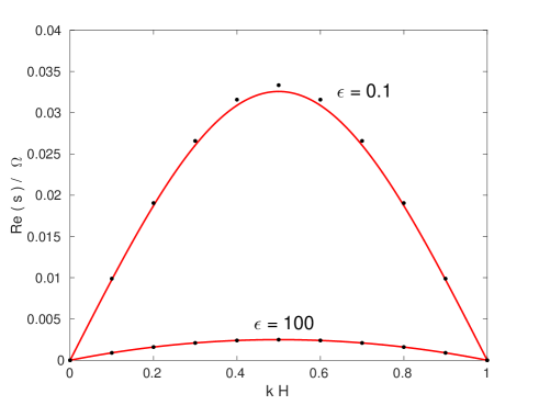
Figure 2: Growth rates of the secular GI in a single fluid for $Q=2$ and two different values of $\epsilon$, 0.1 (weakly coupled) and 100 (strongly coupled). The solid curves represent the full solution to the dispersion relation (14), whereas the points correspond to the asymptotic estimates (18) and (20).

3.4 With gas drag

Being a cubic, the dispersion relation (14) does not yield simple formulae for the various growth rates. It is straightforward, however, to obtain a general stability criterion and asymptotic expressions in the limit of strong and weak drag.

The last term in the cubic reveals that linear instability is assured when $\overline{\omega}^{2}-\Omega^{2}<0$, which is satisifed for all modes with sufficiently small wavenumbers $k<2k_{c}$. Hence instability is unconditional, though in practice (putting aside the disk’s global structure and cylindrical geometric effects) an unstable dust layer must have radial extent greater than $\approx 2\pi/k_{c}$ or else there will insufficient space for the modes to manifest themselves.

In Figure 2 we plot numerical growth rates of the secular GI for parameters characteristic of the two limits. Superimposed are the leading order estimates taken from Eqs (18) and (20) below.

3.4.1 Weak coupling limit

When $\epsilon\ll 1$ we are in the weak drag regime corresponding to larger particles, at larger disk radii, in less massive disks. Eq.(14) then yields two density waves:

$$s=\pm\text{i}\,\overline{\omega}-\frac{1}{2}\Omega\epsilon\left(1+\frac{\Omega^{2}}{\overline{\omega}^{2}}\right)+\mathcal{O}(\epsilon^{2}\Omega),$$ (17)

which are unstable, as expected, when $Q<1$ and thus correspond to the classical GI. Otherwise the two waves are mildly damped by drag.

The third secular mode exhibits a growth rate of

$$s=\frac{\Omega^{2}-\overline{\omega}^{2}}{\overline{\omega}^{2}}\epsilon\Omega+\mathcal{O}(\Omega\epsilon^{2}).$$ (18)

Instability is assured when $\overline{\omega}^{2}<\Omega^{2}$, in accordance with the stability criterion derived above. The fastest growing mode possesses $k=k_{c}$ and the maximum growth rate is

$$s_{\text{max}}\approx\frac{\epsilon\,\Omega}{Q^{2}-1}.$$ (19)

The mode always grows, but for large $Q$ the growth rate can be small.

In the limit of small $\epsilon$, the unstable mode is, in fact, a modified zonal flow. In Eq.(12), the dominant balance is quasi-geostrophic, i.e. between the pressure gradient, self-gravity, and the Coriolis force (because $s\sim\epsilon\Omega$ and $u_{x}\sim\epsilon u_{y}$). Using Eq. (16), with Eqs (11) and (13), gives then precisely the leading order term for $s$.

3.4.2 Strong coupling regime

In the strong drag limit, $\epsilon\gg 1$, the SGI grows at a rate of

$$s=\frac{\Omega^{2}-\overline{\omega}^{2}}{\Omega}\,\epsilon^{-1}+\mathcal{O}(\Omega\epsilon^{-2}).$$ (20)

Instability occurs for the exact same range of $k$ as in the opposed weak drag limit, but the maximum growth rate is slightly altered

$$s_{\text{max}}\approx\frac{\Omega}{Q^{2}\epsilon}.$$ (21)

and the mode works through a different arrangement of forces. In Eq. (12) instead of radial geostrophic balance, it is the last three terms that are dominant: radial contraction by self-gravity is met by the drag force and pressure. Essentially, the dust has achieved terminal velocity. Solving for $u_{x}^{\prime}$ and using (11) yields the leading term for $s$.

In addition, there exist two density waves with $s=\pm\text{i}\overline{\omega}+\mathcal{O}(\epsilon^{-1}\Omega)$. As in the weak coupling limit, they grow exponentially when $Q<1$ but are otherwise weakly damped by drag at a rate $\sim\Omega/\epsilon$.

3.4.3 Role of turbulent diffusion

For completeness we next consider the impact of turbulent mass diffusivity, focussing especially on the critical wavenumber at which instability is quenched. Letting $D\neq 0$, and taking the limit of weak drag, $\epsilon\ll 1$, the leading order expression for the growth rate (18) picks up a term $-k^{2}D\Omega^{2}/\overline{\omega}^{2}$. The critical $k$ is then easy to compute:

$$k_{\text{crit}}=\frac{2\pi G\sigma_{0}}{c^{2}+D\Omega/\epsilon}.$$ (22)

The importance of turbulent diffusion versus pressure is quantified by $D\Omega/(\epsilon c^{2})$. For weakly coupled particles, this parameter is $\sim\alpha(\eta\epsilon)^{-1}\sim 1$, using the estimates on turbulent diffusion and velocity dispersion from Section 2. This is saying that turbulence is roughly as important as dust pressure, at least in setting the short scale cut-off for SGI. Nonetheless, in the remainder of the paper we often omit diffusion when dealing with weakly coupled particles, primarily in order to derive clean expressions. The neglect of diffusion will not change these results qualitatively, but will introduce order 1 corrections. Instability criteria should then be regarded as necessary conditions, not sufficient, and maximum growth rates should be understood as upper bounds.

In the opposite limit, $\epsilon\gg 1$, the situation is quite different. The growth rate (20) is modified by the term $-k^{2}D$, and the importance of turbulent diffusion on small scales is quantified instead by $\epsilon D\Omega/c^{2}$ which is $\sim\epsilon\gg 1$. As a consequence, the critical cut-off for small particles is completely controlled by turbulence, as shown earlier by Youdin (2011) using a heuristic (but essentially equivalent) argument.

On account of the subdominance of particle pressure in the face of turbulent diffusion when $\epsilon\gg 1$, we may dispense with it entirely. In this case, instability is assured for sufficiently long wavelengths as earlier, with the asymptotic growth given by

$$s=\frac{2\pi G\sigma_{0}}{\epsilon\Omega}k-Dk^{2},$$ (23)

and a maximum growth rate of

$$s_{\text{max}}=\frac{\pi^{2}G^{2}\sigma_{0}^{2}}{\epsilon^{2}\Omega^{2}D}\approx\frac{\Omega}{\epsilon^{2}\alpha_{g}Q_{g}^{2}},$$ (24)

where we have introduced the gas Toomre parameter in the last equality, and set $\alpha\approx\alpha_{g}$ (cf. Section 2.2). The wavelength of maximum growth is $\sim\epsilon\alpha_{g}Q_{g}H_{g}$, where $H_{g}$ is the scale height of the gas disk. Given that in this regime $\epsilon$ is large but $\alpha_{g}$ is small, it can be hard to establish this characteristic length a priori.

Before moving on, it should be highlighted that a turbulent mass-diffusion alters the classical GI in unexpected ways. When $\epsilon=0$ and $D\neq 0$, arbitrarily long wavelengths are rendered unstable, though they grow at negligible rates. On the other hand, mass diffusion cannot completely stabilise short scales - a pressureless turbulent fluid will be unstable for all $k$ (in contrast to the SGI). Introducing turbulent momentum diffusion, however, does kill instability for sufficiently large $k$. We omit details of these calculations.

3.5 Physical picture

As has been commented upon in the literature, the secular GI exhibits two striking features: growth for all finite $Q$, and growth upon arbitrarily small $k$. The latter is especially unexpected given that traditional GI prefers intermediate wavelengths, the longer scales stabilised by the dominant Coriolis force. How does secular GI overcome the epicyclic response at large scales?

Consider two dust rings located at different radii undergoing circular orbital motion. Each ring contains a quantity of angular momentum naturally associated with its home radius. Suppose the rings are displaced radially towards one another other. Though their mutual self-gravitational attraction will attempt to amplify the displacement, the two rings possess an angular momentum incommensurate with their new radial location and hence undergo epicyclic oscillations that thwart any type of gravitational collapse. This is the classical picture of stabilisation at long wavelengths.

Suppose however that there exists a drag force on both dust rings due to interactions with the background gas. Now when the two rings are radially displaced they will exchange angular momentum with the gas, via the last term in Eq. (13). The rings either gain or lose angular momentum until they achieve the amount commensurate with their new radial location. As a result, they do not undergo epicyclic motion, and self-gravity continues to amplify their radial drift towards one another. As the two rings collapse they continuously shed or gain angular momentum as needed. In this way, the epicyclic restoring forces are negated by the drag.

Note that this scenario only works if the gas remains an infinite reservoir of angular momentum, which can be removed or added to with no ramifications. This may be a reasonable approximation in cases where the dust density is far less than the gas density, but on some sufficiently long scale even this must break down. The question then arises: on what range of scales does the secular GI operate upon, and under what circumstances may we take the single fluid approximation? For the smooth running of the SGI, the gas fluid must resist undergoing epicyclic oscillation when perturbed by the dust drag. When and how can this be arranged? These questions will be explored in the following two sections.

4 Two-fluid model: incompressible gas

As an intermediate step between the single fluid and fully compressible two-fluid models, we briefly analyse the case of a compressible dust disk embedded in an incompressible gas. This situation mimics the case when the dust scale height is far less than the gas scale height, and the unstable motions very subsonic. On the vertical scale of the dust disk, the gas density is effectively constant and the problem is ‘vertically local’ as far as the gas is concerned. Consequently, the gas density does not contribute to the perturbed Poisson equation.

4.1 Governing equations

The equations governing the evolution of the incompressible gas are

$$\partial_{t}\mathbf{U}+\mathbf{U}\cdot\nabla\mathbf{U} =-\nabla P_{g}/\sigma_{g}-\nabla\Phi_{t}-\nabla\Phi_{\text{sg}}$$

$$\hskip 28.45274pt-2\Omega\mathbf{e}_{z}\times\mathbf{U}+\epsilon\Omega\frac{\sigma}{\sigma_{g}}(\mathbf{u}-\mathbf{U}),$$ (25)

$$\nabla\cdot\mathbf{U} =0,$$ (26)

where $\sigma_{g}$ and $P_{g}$ are the gas surface density and vertically integrated pressure, within the dust layer. Because the gas is incompressible $\sigma_{g}$ is a constant. As earlier, $\mathbf{U}$ is the gas velocity, and $\mathbf{u}$ is the dust velocity. The equations governing the dust fluid are those that appear in Section 2, Eqs (8)-(10). To ease the analysis $D=0$.

4.2 Dispersion relation

Once again, we assume the standard equilibrium state $P_{g}=P_{g0}$, $\sigma=\sigma_{0}$, $\mathbf{u}=\mathbf{U}=-(3/2)\Omega\,x\mathbf{e}_{y}$, where the gas pressure and dust surface density is constant. Next, axisymmetric perturbations are assumed, denoted by $\mathbf{U}^{\prime}$, $P_{g}^{\prime}$, $\mathbf{u}^{\prime}$, $\sigma^{\prime}$, and these are taken to be $\propto\text{exp}(st+\text{i}kx)$.

Because of the incompressibility condition we immediately obtain $U_{x}^{\prime}=0$, and $U_{y}^{\prime}$ is computed from the $y$-force balance, yielding

$$U_{y}^{\prime}=\frac{\epsilon\,\delta\,\Omega}{s+\epsilon\,\delta\Omega}u_{y}^{\prime},$$ (27)

where we have introduced now $\delta=\sigma_{0}/\sigma_{g}$ which quantifies the dust-to-gas density ratio for a given particle size. This equation states that the gas is azimuthally accelerated by dust drag. Simultaneously, a form of radial geostrophic balance holds for the gas, with the Coriolis force balanced by the radial pressure pressure, self-gravity, and drag. Importantly, the gas pertubation cannot undergo epicyclic motion, which might impede the growth of the secular GI. The gas pressure gradient holds the fluid radially ‘in place’ and a sequence of azimuthal jets ensues, each accelerated by the dust drag. (Note that the absence of epicycles is a generic feature of incompressible flow confined to the orbital plane.)

The perturbation equations for the dust are the same as Eqs (11)-(13) except for the inclusion of the term $\epsilon\Omega U_{y}^{\prime}$ on the right side of the dust’s $y$-force balance. Eliminating the dependent variables obtains the following quartic dispersion relation:

$$s^{4}+(2+\delta)\epsilon\Omega\,s^{3}+[\overline{\omega}^{2}+(1+3\delta)\epsilon^{2}\Omega^{2}]s^{2}$$

$$\hskip 56.9055pt+\epsilon\Omega\left[\delta(\overline{\omega}^{2}+2\epsilon^{2}\Omega^{2})+\overline{\omega}^{2}-\Omega^{2}\right]s$$

$$\hskip 113.81102pt+2\delta(\overline{\omega}^{2}-\Omega^{2})\epsilon^{2}\Omega^{2}=0,$$ (28)

which we now briefly analyse.

4.3 Instability criterion and asymptotic growth rates

Though Eq. (28) may appear rather formidable, an instability criterion appears immediately. Putting aside the clasical GI for now, the SGI mode is marginal when the last term is zero, yielding exactly the same instability criterion as in the single fluid model: $\overline{\omega}^{2}<\Omega^{2}$, and hence instability occurs on all $k<2k_{c}$. Though we allow for gas perturbations, gas incompressibility restricts these to a form of zonal flow which absorbs or bestows angular momentum as necessary to faciliate instability in the dust.

In the weak coupling limit, $\epsilon\ll 1$, the leading order term in the SGI growth rate is obtained by setting $s=s_{1}\epsilon+\dots$ and substituting this into (28). One obtains the quadratic:

$$s_{1}^{2}+\Omega(\delta-\xi)s_{1}-2\delta\frac{(\Omega^{2}-\overline{\omega}^{2})}{\overline{\omega}^{2}}\Omega^{2}=0.$$ (29)

The resulting solution for $s_{1}$ agrees with the single fluid expression (18) to leading order in small dust-to-gas fraction $\delta<1$. The reason for the dependence on $\delta$ is because the ability to transfer angular momentum between gas and dust is influenced by the relative azimuthal speeds of the two fluids, which depends on $\delta$ via (27).

In the strong coupling limit, $\epsilon\gg 1$, assuming that $s\sim\Omega/\epsilon$, a similar analysis reveals that the SGI growth does not depend on $\delta$ at all. In fact, $s=(\Omega^{2}-\overline{\omega}^{2})/(\epsilon\Omega)$, precisely the same expression as in the single fluid case (20).

5 Two-fluid model: compressible gas

Having treated simpler models of the dust-gas system, we turn to a fully compressible two-fluid approach, informed by what we have learned so far. The sound speed of the gas $c_{g}$ and its scale height $H_{g}=c_{g}/\Omega$ are assumed finite, with the dust subdisk embedded in the gas, so that $c<c_{g}$ and $H<H_{g}$. As in the previous section, we average over the vertical thickness of the dust disk, and thus neglect complications arising on the smaller scales $<H$, such as shear instabilities and turbulence. These are included in an ad hoc way, using a turbulent mass diffusivity and enhanced dust pressure. Perhaps more importantly, the gas outside the dust disk is completely neglected as far as the onset of instability is concerned. The external gas is ‘inert’ — both gravitationally and dynamically decoupled. The resulting model is workable but suffers the shortcomings discussed previously in Section 2.

5.1 Governing equations

We adopt the equations listed in TI in order to describe our system:

$$\partial_{t}\sigma+\mathbf{u}\cdot\nabla\sigma =-\sigma\nabla\cdot\mathbf{u}+D\nabla^{2}\sigma,$$ (30)

$$\partial_{t}\mathbf{u}+\mathbf{u}\cdot\nabla\mathbf{u} =-\frac{1}{\sigma}\nabla P-\nabla\Phi_{t}-\nabla\Phi_{\text{sg}}$$

$$\hskip 28.45274pt-2\Omega\mathbf{e}_{z}\times\mathbf{u}+\epsilon\Omega(\mathbf{U}-\mathbf{u}),$$ (31)

$$\partial_{t}\sigma_{g}+\mathbf{U}\cdot\nabla\sigma_{g} =-\sigma_{g}\nabla\cdot\mathbf{U},$$ (32)

$$\partial_{t}\mathbf{U}+\mathbf{U}\cdot\nabla\mathbf{U} =-\frac{1}{\sigma_{g}}\nabla P_{g}-\nabla\Phi_{t}-\nabla\Phi_{\text{sg}}$$

$$\hskip 28.45274pt-2\Omega\mathbf{e}_{z}\times\mathbf{U}+\epsilon\Omega\frac{\sigma}{\sigma_{g}}(\mathbf{u}-\mathbf{U}),$$ (33)

$$\nabla^{2}\Phi_{\text{sg}} =4\pi G(\sigma+\sigma_{g})\delta(z).$$ (34)

Both dust and gas are assumed isothermal, so that $P=\sigma c^{2}$ and $P_{g}=\sigma_{g}c_{g}^{2}$. As mentioned, by assuming that the dust and gas enclosed in $|z|<H$ is razor thin, we omit the gravitational influence of gas external to the dust disk. As a consequence, $\sigma_{g}$ should be understood as the surface density of the gas located within the vertical extent of the dust subdisk.

5.2 Dispersion relation

Once again we assume a simple background equilibrium of homogeneous density and Keplerian shear: $\sigma=\sigma_{0}$, $\sigma_{g}=\sigma_{g0}$, $\mathbf{u}=\mathbf{U}=-(3/2)\Omega x\mathbf{e}_{y}$. To this we add disturbances, denoted by primes, that are $\propto\text{exp}(st+\text{i}kx)$. The resulting linearised equations are:

$$s\sigma^{\prime} =-\sigma_{0}\text{i}ku_{x}^{\prime}-Dk^{2}\sigma^{\prime},$$ (35)

$$su_{x}^{\prime} =-\text{i}kc^{2}(\sigma^{\prime}/\sigma_{0})+2\Omega u_{y}^{\prime}-\text{i}k\Phi^{\prime}+\epsilon\Omega(U_{x}^{\prime}-u_{x}^{\prime}),$$ (36)

$$su_{y}^{\prime} =-\tfrac{1}{2}\Omega u_{x}^{\prime}+\epsilon\Omega(U_{y}^{\prime}-u_{y}^{\prime}),$$ (37)

$$s\sigma_{g}^{\prime} =-\sigma_{g0}\text{i}kU_{x}^{\prime},$$ (38)

$$sU_{x}^{\prime} =-\text{i}kc_{g}^{2}(\sigma_{g}^{\prime}/\sigma_{g0})+2\Omega U_{y}^{\prime}-\text{i}k\Phi^{\prime}+\epsilon\delta\Omega(u_{x}^{\prime}-U_{x}^{\prime}),$$ (39)

$$sU_{y}^{\prime} =-\tfrac{1}{2}\Omega U_{x}^{\prime}+\epsilon\delta\Omega(u_{y}^{\prime}-U_{y}^{\prime}),$$ (40)

where the equilibrium dust-to-gas density ratio is $\delta=\sigma_{0}/\sigma_{g0}$ for a given size $a$. Finally, the perturbed gravitational potential is obtained from

$$\Phi^{\prime}=-(2\pi G/|k|)(\sigma^{\prime}+\sigma_{g}^{\prime}).$$

The system of equations (35)-(40) yields a rather involved 6th order dispersion relation:

$$s^{6}+a_{5}s^{5}+a_{4}s^{4}+a_{3}s^{3}+a_{2}s^{2}+a_{1}s+a_{0}=0,$$ (41)

with

$$a_{5} =2(1+\delta)\epsilon\Omega+Dk^{2},$$

$$a_{4} =(1+\delta)^{2}\epsilon^{2}\Omega^{2}+\overline{\omega}^{2}+\overline{\omega}^{2}_{g}+2(1+\delta)\epsilon\Omega Dk^{2},$$

$$a_{3} =\epsilon\Omega\left[(1+\delta)2\mu^{2}-\delta c_{g}^{2}k^{2}+(1+2\delta)c^{2}k^{2}\right]$$

$$\hskip 56.9055pt+\left[(1+\delta)^{2}\epsilon\Omega^{2}+\overline{\omega}^{2}_{g}+\Omega^{2}\right]Dk^{2},$$

$$a_{2} =c^{2}k^{2}\overline{\omega}_{g}^{2}+\Omega\mu^{2}-2c_{g}^{2}k^{2}\pi G\sigma_{0}|k|$$

$$\hskip 28.45274pt+(1+\delta)\epsilon^{2}\Omega^{2}\left[(1+\delta)\mu^{2}+\delta c^{2}k^{2}-\delta c_{g}^{2}k^{2}\right]$$

$$\hskip 56.9055pt+\left[2(1+\delta)\overline{\omega}_{g}^{2}-c_{g}^{2}k^{2}\right]\epsilon\Omega Dk^{2},$$

$$a_{1} =\epsilon\Omega k^{2}\left[\delta c_{g}^{2}(\mu^{2}-c_{g}^{2}k^{2})+c^{2}(\mu^{2}+\delta c_{g}^{2}k^{2})\right]$$

$$\hskip 28.45274pt+\left\{\overline{\omega}_{g}^{2}\left[1+\epsilon^{2}(1+\delta)^{2}\right]-\epsilon^{2}\delta(1+\delta)c_{g}^{2}k^{2}\right\}Dk^{2}\Omega^{2},$$

$$a_{0} =Dc_{g}^{2}k^{4}\delta\epsilon\Omega^{3}.$$

In order to ease the presentation of the coefficients we have introduced the following frequencies

$$\overline{\omega}_{g}^{2} =\Omega^{2}-2\pi G\sigma_{g0}|k|+c_{g}^{2}k^{2},$$

$$\mu^{2} =\Omega^{2}-2\pi G(\sigma_{g0}+\sigma_{0})|k|+c_{g}^{2}k^{2}.$$

Recall that $\overline{\omega}^{2}$ is the squared frequency of density waves in the dust fluid given by Eq. (15).

5.3 No turbulent mass diffusion

In this subsection we analyse the case when mass diffusion in the continuity equation is negligible, $D\approx 0$, but we retain the velocity dispersion of the dust particles. This situation may adequately describe a disk of weakly or marginally coupled dust and gas, $\epsilon\lesssim 1$. For this case the dust disk is expected to be thinner and ‘colder’ than the gas disk, and so $\eta=c^{2}/c_{g}^{2}\ll 1$. However, because of the omission of mass diffusion, the instability conditions derived here should be regarded as necessary, not sufficient, and maximum growth rates understood as upper bounds.

5.3.1 Instability criterion

When $D=0$ the dispersion relation (41) reduces to a quintic. Marginality corresponds then to $a_{1}=0$, which provides us with a condition for the onset of instability. In fact $a_{1}=0$ is a quadratic equation for $k$,

$$c^{2}c_{g}^{2}k^{2}-2\pi G\sigma_{g0}(c^{2}+\delta c_{g}^{2})|k|+(c^{2}+c_{g}^{2}\delta)/(1+\delta)=0,$$ (42)

indicating that if instability occurs it takes place on a range of wavenumbers $k_{1}<k<k_{2}$, where $k_{1}$ and $k_{2}$ are solutions to the quadratic. In order for such a range to exist, the critical $k$’s must be real. This is the case when the discriminant of (42) is positive, and the instability criterion proceeds easily:

$$Q_{g}\equiv\frac{\Omega c_{g}}{\pi G\sigma_{g0}}<\sqrt{\frac{(1+\delta)(\delta+\eta)}{\eta}}\lesssim\sqrt{1+\frac{\delta}{\eta}},$$ (43)

where the last scaling arises if $\delta<1$. Alternatively, the criterion can be reworked in terms of the dust’s Toomre parameter, noting that $Q=\sqrt{\eta}\delta^{-1}Q_{g}$. We then obtain instability when

$$Q\lesssim\frac{\sqrt{\delta+\eta}}{\delta}\approx\delta^{-1/2},$$ (44)

where in the last approximation we assume that $\eta\ll\delta$ (always the case, unless turbulence is absent— see Section 2.2).

However expressed, this simple criterion encapsulates clearly the main physical effects. For instance, if we take the limit of negligible dust, $\delta\to 0$, the instability criterion become simply $Q<\infty$, and the system is always unstable. In this limit the dust’s drag on the gas is unimportant and the the two-fluid system reproduces the same stability behaviour as the single fluid model (Section 3): the Toomre parameter does not feature.

For general $\delta$, however, stability in the two-fluid disk does in fact depend on the gas’s (or dust’s) Toomre parameter: if it is too large then instability is switched off. If $\delta/\eta\gg 1$, the instability criterion may be written as

$$Q_{g}\lesssim\frac{c_{g}}{c}\left(\frac{\sigma_{0}}{\sigma_{g0}}\right)^{1/2}\approx\left(\epsilon\alpha_{g}\right)^{-1/2}\left(\frac{\sigma_{0}}{\sigma_{g0}}\right)^{1/2},$$ (45)

which may greatly exceed the classical value of 1, allowing instability to occur in a finite range of conditions. In this case we recover the secular GI.

5.3.2 Asymptotic growth rates

Explicit expressions for the growth rate are possible in the limit of $\epsilon\ll 1$. We set aside the classical GI and isolate the SGI mode by setting $s=s_{1}\epsilon+\dots$. Collecting terms of order $\epsilon$, we obtain

$$s_{1}=\left(\frac{\sigma_{0}}{\sigma_{g0}}\right)\left(\frac{2\pi G\sigma_{g0}|k|-\Omega^{2}}{\overline{\omega}_{g}^{2}}\right)\left(\frac{k^{2}c_{g}^{2}}{\Omega}\right)-\frac{k^{2}c^{2}}{\Omega},$$ (46)

to leading order in small $\delta$ and $\eta$. The last damping term arises from the particle pressure and kicks in at short scales, of order $H=c/\Omega$. Instability is thus restricted to scales longer than $H$. Conversely, the Coriolis force acting on the gas (represented by the $\Omega^{2}$) stabilises long wavelengths, so that instability only occurs on scales shorter than $\approx 2\pi G\sigma_{g0}/\Omega^{2}$ (as in classical GI). The stabilising effect of gas pressure, on the other hand, does not make an appearance. In summary, instability occurs on a range of intermediate scales. But for this range of unstable wavelengths to exist, the dust pressure must be sufficiently weak or else the last term in (46) swallows the first term.

Expression (46) can be further simplified if we restrict our attention to lengthscales much shorter than the gas’s Jeans length $\sim c_{g}^{2}/(G\sigma_{g0})$, but not so short that the dust pressure dominates the other processes. In other words, we require $G\sigma_{g0}/c_{g}^{2}\ll k\ll G\sigma_{0}/c^{2}$. If this intermediate range exists, then on it we may approximate $\overline{\omega}_{g}^{2}\approx k^{2}c_{g}^{2}$ in the denominator of the first term in (46), and obtain

$$s\approx\frac{\Omega^{2}-\overline{\omega}^{2}}{\Omega}\,\epsilon-\delta\epsilon\Omega.$$ (47)

Assuming further than $\delta\ll 1$ the last term may be dropped and we have an expression similar to the single fluid one, (18). The maximum growth rate is easy to compute:

$$s_{\text{max}}\approx\frac{\epsilon\Omega}{Q^{2}},$$ (48)

using the Toomre parameter for the dust. This expression is consistent with Eq. (19), for sufficiently large $Q$. But note that it only holds if there is a sufficient separation of scales between the dust and gas pressure scale heights, which is assured if $\eta\ll\delta$. The wavelength of maximum growth is also similar to that in a single fluid $\sim QH$.

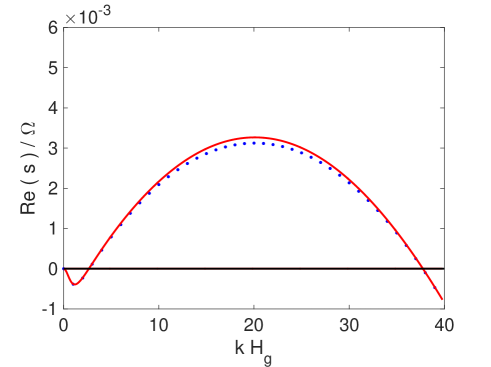
Figure 3: Growth rate of the SGI as a function of radial wavenumber $k$ for weakly coupled particles. Parameters are $Q_{g}=5$, $\epsilon=0.1$, $\delta=0.01$, and $\eta=10^{-4}$. Here $H_{g}=c_{g}/\Omega$ is the gas vertical scale height. The solid red line is the full solution to the dispersion relation and the blue dotted solution is the asymptotic growth rate from (46)

In Fig. 3 we plot the asymptotic growth rate as a function of $k$ alongside the full solution obtained numerically from (41). For the parameters chosen the agreement is respectable, but naturally worsens once we leave the asymptotic regime of small $\delta$, $\eta$, and $\epsilon$. Note that the lengthscale of fastest growth is less than the gas-disk thickness $\sim(\pi/10)H$, though much longer than the particle-disk thickness because $H/H_{g}\sim 10^{-2}$.

5.4 Pressureless turbulent dust

Having treated the non-turbulent case, more relevant for weakly coupled particles, we now turn to a pressureless dust suspended in a turbulent gas disk, the regime that best describes small dust. Thus in Eqs (35)-(40) we set $D\neq 0$, but $c=0$, and it is assumed that $\epsilon\gg 1$. In addition, the turbulent diffusion is presumed small, $\alpha\ll 1$. The simplest way to capture the full effects of diffusion is to let $Dk^{2}\sim\epsilon^{-1}\Omega$, which (whatever the value of $D$) will be true on some radial lengthscale. On longer wavelengths persisting with this scaling means we include harmless subdominant terms, while on shorter wavelengths we expect diffusion to quench instability in any case. The resulting equations correspond exactly to those treated in Sections 2 and 3 in TI, which we now analyse in more detail and give explicit expressions for the growth rates.

5.4.1 Instability criterion

When $D\neq 0$, the onset of instability is difficult to calculate from the dispersion relation because unstable modes possess (small) complex frequencies. Some progress can be made, however, in the limit of $\epsilon\gg 1$ and assuming that $s=\epsilon^{-1}s_{1}+\dots$ (thus extracting only SGI modes) and $\alpha_{g}=\epsilon^{-1}\alpha_{1}+\dots$. Recall from Section 2.2 that in the tight coupling limit $\alpha\approx\alpha_{g}$. To leading order the dispersion relation (41) becomes the quadratic

$$(1+\delta)\left[(1+\delta)\mu^{2}-\delta c_{g}^{2}k^{2}\right]\Omega^{2}s_{1}^{2}-\left\{\delta c_{g}^{2}(\mu^{2}-c_{g}^{2}k^{2})\right.$$

$$\hskip 28.45274pt\left.+\alpha_{1}(1+\delta)\left[(1+\delta)\overline{\omega}^{2}-\delta c_{g}^{2}k^{2}\right]\right\}k^{2}c_{g}^{2}\Omega s_{1}$$

$$\hskip 56.9055pt+\delta c_{g}^{4}k^{4}\alpha_{1}\Omega^{2}=0.$$ (49)

In Eq. (13) TI present an equivalent expression. For reasonable values of $\delta$ and $Q_{g}>1$ the coefficient of $s_{1}^{2}$ is positive and so the sign of the growth rates can be determined from the coefficient of $s_{1}$. After some manipulation the instability criterion is

$$Q_{g}<[\delta+\epsilon\alpha_{g}(1+\delta)]\sqrt{\frac{1+\delta}{\epsilon\alpha_{g}\left[\delta+\epsilon\alpha_{g}(1+\delta)^{2}\right]}},$$ (50)

which agrees with Eq. (18) in TI. Taking small $\delta$, this simplifies to

$$Q_{g}\lesssim\sqrt{1+\frac{\delta}{\epsilon\alpha_{g}}},$$ (51)

which is remarkably similar to the diffusionless criterion (43). The smaller the turbulent diffusion $\alpha_{g}$, the greater the range of instability. Diffusion on small scales has replaced dust pressure in (43) in stabilising the secular GI, but the two processes work exactly the same otherwise. Finally, note that (51) differs from the final criteria in TI because they make additional and unnecessary assumptions regarding the relative sizes of $\epsilon$, $\delta$, and $\alpha_{g}$.

5.4.2 Asymptotic growth rates

Solutions to the quadratic (49) are ugly, but if we take the limit $\delta\ll 1$, we obtain

$$\text{Re}(s)=\frac{1}{2}\left(\frac{\sigma_{0}}{\sigma_{g0}}\right)\left(\frac{2\pi G\sigma_{g0}|k|-\Omega^{2}}{\epsilon\,\overline{\omega}_{g}^{2}}\right)\left(\frac{k^{2}c_{g}^{2}}{\Omega}\right)-\frac{1}{2}k^{2}\alpha.$$ (52)

This is almost identical to expression (46). The main difference is that the stabilising term on short scales arises from turbulent diffusion, rather than dust pressure, once again. The long wavelength stabilisation is the same — the Coriolis force. Instability can only occur if these two stabilising scales are sufficiently well separated.

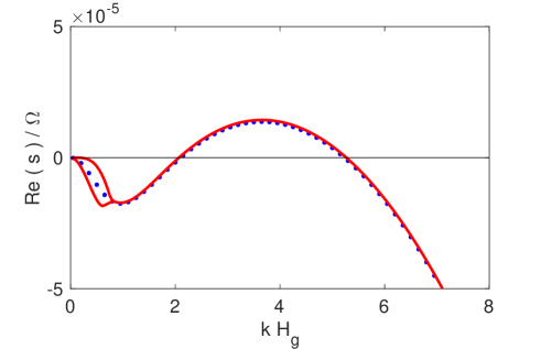
Figure 4: Growth rate of the SGI as a function of $k$ for tightly coupled particles. Parameters are: $Q_{g}=3$, $\epsilon=100$, $\delta=0.01$, and $\alpha=10^{-5}$. The solid red line is the full solution to the dispersion relation, and the blue dots correspond to the asymptotic growth rate (52).

In Fig. 4 we plot the asymptotic growth rate (52) as a function of $k$ next to the full solution obtained numerically from (41). For a representative set of parameters the agreement is good, though weakens the smaller $\epsilon$ and the larger $\delta$, as expected. Note also that at small $k$ the approximation fails to capture the bifurcation into two monotonically growing modes with different growth rates. Finally, the wavelength of fastest growth is $\sim H_{g}$, and thus the approximation of a razor thin disk is only marginally applicable.

The approximate maximum growth rate can be obtained by a similar argument to that given in Section 5.3.2. We find to leading order on the intermediate range $G\sigma_{g0}/c_{g}^{2}\ll k\ll G\sigma_{0}/(\epsilon\alpha\Omega)$ and for $\delta\ll 1$ that

$$s\approx\frac{1}{2}\frac{\pi G\sigma_{0}|k|}{\epsilon\Omega}-k^{2}\alpha.$$ (53)

This expression is similar to the growth rate in the single-fluid pressureless case, (23), differing only by a half (on account of the unstable mode appearing as a complex conjugate pair). The maximum growth rate is staightforward to compute, and we find

$$\text{Re}(s_{\text{max}})=\frac{1}{2}\frac{\pi^{2}G^{2}\sigma_{d}^{2}}{\epsilon^{2}\alpha}=\frac{1}{2}\frac{\Omega}{\epsilon^{2}\alpha_{g}Q_{g}^{2}},$$ (54)

with maximum growth occuring on lengthscales $\sim\epsilon\alpha_{g}Q_{g}H_{g}$(as in the single fluid). Note that a similar expression to (53) (and identical to (24)) can also be achieved by enforcing the terminal velocity approximation for the dust in Eq. (36), and then radial geostrophic balance for the gas in Eq. (39). The latter assumption, combined with the remaining equations, ensures that $U_{x}^{\prime}\sim\delta u_{x}^{\prime}$ and so, to leading order, the growth rate is the same as in the single fluid treatment.

5.5 Physical picture

To complete this section we bring together the insights gained from the preceding analyses and construct a physical model for how the secular GI works in a two-fluid disk. As is clear from the asymptotic estimates (46) and (52), instability occurs only when there exists a range of intermediate wavelengths in which both the gas’s tidal forces and dust pressure/turbulence are sufficiently weak. Obviously, dust pressure or turbulence will interfere with gravitational collapse on small scales, stopping the clumping of material into rings. Instability hence migrates to longer scales where this effect is weak. On sufficiently long scales, however, the tidal force will send a disturbed gas parcel into epicyclic motion, which also impedes clumping. To counteract this effect, instability must then move to shorter scales where the gas pressure is sufficiently strong to block the gas’s epicyclic tendency (via a zonal, or geostrophic, flow). Criteria (43) and (51) describe necessary conditions that permit some band of wavelengths to satisfy these two requirements.

Essentially, the two-fluid mode is attempting to be as close to the single-fluid model (Section 3) or the two-fluid incompressible model (Section 4) as possible. On this intermediate range of lengthscales two dust blobs radially displaced towards one another exchange their angular momentum with the background gas, and hence can gravitationally collapse rather than be sent into epicycles. The gas, however, being no longer an infinite reservoir of angular momentum undergoes a commensurate perturbation. If the gas pressure is sufficiently strong, however, this perturbation takes the form of a zonal flow, not an epicycle, and so the structure of the instability is retained. If we move to longer and longer scales, the gas pressure weakens and so can only support very mild zonal flows, unable to carry appreciable angular momentum from the drifting dust. As a consequence, the instability is suppressed. On the other hand, whereas the gas is in radial geostrophic balance, the dust can fall into either geostrophic balance (for $\epsilon\ll 1$) or terminal velocity balance (for $\epsilon\gg 1$).

6 Discussion

In this section we apply the stability criteria and growth rate estimates of the two-fluid model to reasonable models of protoplanetary disks. Because of uncertainties in the parameters and deficiencies in the model itself, we do not attempt to be comprehensive or to hold fast to the quantitative results we obtain. Rather the aim is to give a sense of the main trends and qualitative behaviour, and the general range of numbers one might find in a real system. To that purpose we first concentrate on the two populations of strongly and marginally coupled particles, using the simple estimates derived previously. We then solve the full dispersion relationship numerically at each radius.

The disk model we use is a variant of the minimum mass solar nebula (see Youdin 2011). The background gas disk surface density is given as a function of disk radius by

$$\sigma_{0}=2\times 10^{3}FR_{\text{AU}}^{-3/2}\,\text{g cm}^{-2}.$$ (55)

Here $F$ is a free dimensionless parameter, and $R_{\text{AU}}$ is disk radius in units of AU. The temperature of the nebula is given by

$$T=200\,R_{\text{AU}}^{-1/2}\,\text{K}.$$ (56)

As a consequence, the gas’s Toomre parameter is

$$Q_{g}\approx\frac{40}{F}R_{\text{AU}}^{-1/4}.$$ (57)

Thus at 1 AU, $Q_{g}$ is roughly 40 and this falls to about 10 as we approach 100 AU. The inverse Stoke’s number can be approximated by

$$\epsilon=4\times 10^{3}\frac{F}{a_{\text{mm}}}R_{\text{AU}}^{-3/2},$$ (58)

where $a_{\text{mm}}$ is particle size in units of mm. We have assumed that the particles always lie in the Epstein regime. Only the largest particles at the smallest radii enter the Stokes drag regime, so to make life simple we omit it. As a result, stability can be determined once $\delta$, $F$, $\alpha_{g}$, particle size, and the disk radius are specified.

6.1 Weakly coupled particles

First consider larger particles with a largish Stokes number $\epsilon\lesssim 1$. From Figure 1, in a standard MMSN these might correspond to $\sim$ 10 cm particles at 30 AU or more or $\sim 1$ cm particles at 100 AU. In an older less massive disk, this class may also include mm particles but only at 100 AU. Thus most particles do not fall into this regime.

Secular GI arises when criterion (45) is fulfilled. Taking the standard value for the dust to gas ratio $\delta=10^{-2}$, we only need to estimate the ratio of velocity dispersions. Assuming that the particles’ random motions are controlled by the background turbulence, as in Section 2, we have $c/c_{g}\sim\sqrt{\epsilon\alpha_{g}}$ and thus instability occurs when

$$Q_{g}<Q_{\text{crit}}\approx 10^{-1}\epsilon^{-1/2}\alpha_{g}^{-1/2}.$$ (59)

This criterion includes both the classical GI of a dust layer and the secular GI, in which we are more interested. As discussed earlier, the properties of the turbulence are poorly constrained. We thus allow $\alpha_{g}$ to vary between $10^{-7}$ (a perhaps unrealistically low level) and $10^{-3}$. Next, to fix ideas, we set $\epsilon\sim 0.1$ and find that the critical Toomre parameter for the gas is

$$Q_{\text{crit}}\approx 10-10^{3},$$

with the lower value corresponding to a thick disk of relatively ‘hot’ particles ($\alpha_{g}=10^{-3}$), and the higher value to a thin disk of colder particles ($\alpha_{g}=10^{-7}$).

Our standard MMSN with $F=1$ yields $Q_{g}$ that fall directly in this range. If $\alpha_{g}=10^{-3}$ instability is not possible, but if $\alpha_{g}\geq 10^{-4}$ then instability can occur on most radii. Less massive disks exhibit larger $Q_{g}$; for instance with $F=0.1$, we have $Q_{g}>100$ at all radii, and thus the existence of SGI is very much conditional on the efficiency of the turbulence. If $\alpha_{g}\sim 10^{-7}$ then cm sized particles, or even smaller, could be unstable in the outer regions of low mass disks.

What of the growth rates of the unstable modes? Equation (48) gives an upper bound on $s$, in the regime of larger particles. This can be reworked into

$$s_{\text{max}}\approx\delta^{2}Q_{g}^{-2}\alpha_{g}^{-1}\Omega\sim 10^{-6}\alpha_{g}^{-1}\Omega,$$ (60)

where the last equality comes by setting $\delta=10^{-2}$ and $Q_{g}\sim 10$. For relatively strong turbulence $\alpha_{g}\sim 10^{-4}$, the e-folding time of an unstable mode is $10^{2}$ orbits, too long to be relevant at 100 AU, but possibly significant at smaller radii, for example 10 cm size particles at $\sim 10$ AU. Smaller $\alpha_{g}$, of course, yield faster growth on relevant timescales.

6.2 Tightly coupled particles

We next consider well coupled particles, a class that covers most solids of interest (see Figure 1). The relevant stability criterion for this dust is given by (51). The dimensionless diffusion coefficient for tightly coupled particles is $\alpha\approx\alpha_{g}$. Setting $\delta=0.01$ and $\epsilon=10$ yields the criterion

$$Q_{g}\lesssim\sqrt{1+10^{-3}\alpha_{g}^{-1}},$$ (61)

which is more difficult to satisfy than in the weakly coupled case. If we assume that $\alpha_{g}=10^{-7}-10^{-3}$, the condition becomes

$$Q_{g}<Q_{\text{crit}}\approx 1-100,$$

where the larger value corresponds to inefficient turbulent diffusion ($\alpha_{g}=10^{-7}$) and the lower bound corresponds to efficient diffusion ($\alpha_{g}=10^{-3}$). Once again, this suggests that instability occurs when the turbulence is sufficiently weak. In fact, given $F=1$, the SGI is suppressed if $\alpha_{g}\geq 10^{-5}$. The situation worsens when $\epsilon>10$. The conclusion is that the instability may not be widespread in smaller dust.

Let us next turn to growth rates, in particular expression (54). To fix some numbers, we generously set $\epsilon=10$ and $\delta=0.01$ and after some manipulation obtain

$$\text{Re}(s_{\text{max}})\sim 10^{-6}Q_{g}^{-2}\alpha_{g}^{-1}\Omega.$$

If $Q_{g}\sim 10$, then we have

$$\text{Re}(s_{\text{max}})\sim 10^{-8}\alpha_{g}^{-1}\Omega.$$ (62)

While $\alpha_{g}\leq 10^{-7}$ yields appreciable growth at all radii, $\alpha_{g}=10^{-6}$ does so only for $R\lesssim 10$ AU. For larger $\epsilon$ growth times lengthen. This further reinforces the conclusion that the SGI is only relevant to the dynamics of tightly coupled particles when turbulence is very low indeed.

6.3 Marginally coupled particles in realistic disk models

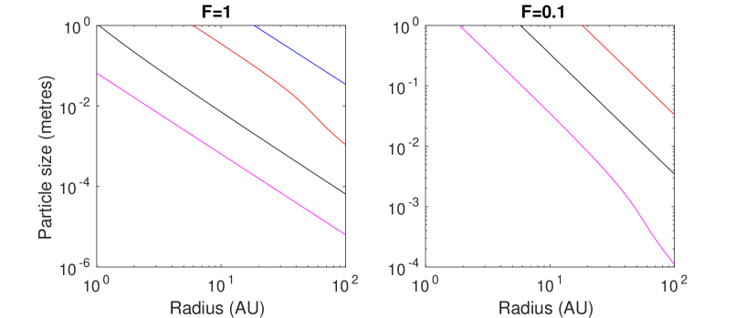
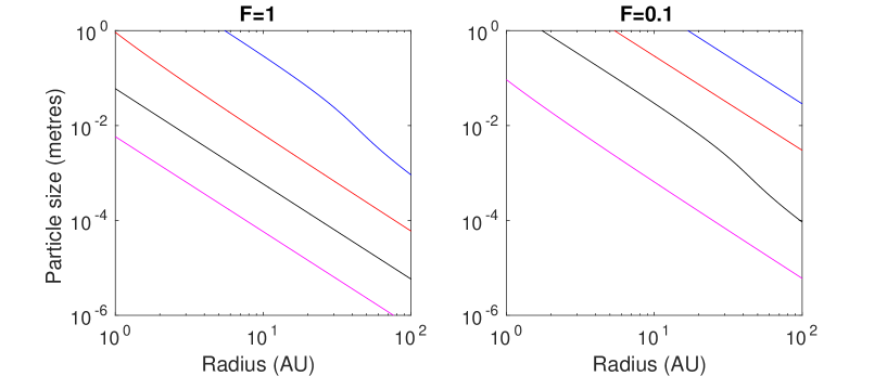
Figure 5: Stability curves in a plane of disk radius and particle size. The pink, black, red, and blue curves correspond to $\alpha_{g}=10^{-7},\,10^{-6},\,10^{-5},\,10^{-4}$. The regions above the respective curves are unstable. Two disk models are employed, a more massive disk with $F=1$ (left panels) and a less massive disk with $F=0.1$ (right panels). The upper row corresponds to a dust-to-gas mass ratio of $\delta=0.01$, while the lower row to $\delta=0.1$.

In this subsection we solve the full dispersion relation at each radius of our disk model. Figure 1 indicates that particle sizes of a mm and above couple to the gas differently at different radii, potentially passing from the well-coupled to the weakly coupled regimes as we go further out radially. At certain radii $\epsilon\sim 1$ and our analytic results are no longer strictly valid, meaning that the dispersion relation (41) must be solved numerically.

Some stability curves are plotted in Fig. 5 for two different disk models, $F=1$ (left panels) and $F=0.1$ (right panels), for several values of the turbulence parameter $\alpha_{g}$, and for two values of the dust to gas density ratio, $\delta=0.01$ (top row) and $0.1$ (bottom row). Parameter regions above a given curve are subject to instability, and thus for a given $\alpha_{g}$ and particle size there exists a critical radius within which the SGI is completely suppressed. In fact, for a relatively turbulent disk with $\alpha_{g}=10^{-4}$, $F=1$ and $\delta=0.01$, all particles smaller than $\approx 3$ cm are stable, and all particles smaller than 1 mm, when $\alpha_{g}=10^{-5}$. Weaker levels of turbulence, of course, permit instability upon smaller particle sizes and for larger swathes of the disk. But one must drive $\alpha_{g}$ to levels $\sim 10^{-7}$ to obtain SGI at radii $<10$ AU for particles larger than a mm.

The SGI’s struggles worsen when the disk is less massive ($F=0.1$), with mm sized particles unstable only for very low values of $\alpha_{g}$. But moving to the lower row of plots, it is immediately clear that increasing $\delta$ improves its range. For example, if $F=1$ and $\alpha_{g}=10^{-4}$ then all particles smaller than mm sizes are stable. If $\alpha_{g}=10^{-5}$ then all particles smaller than $\sim 0.1$ mm are stable. On the other hand, when $\delta<0.01$ the prospects for instability become increasingly bleak.

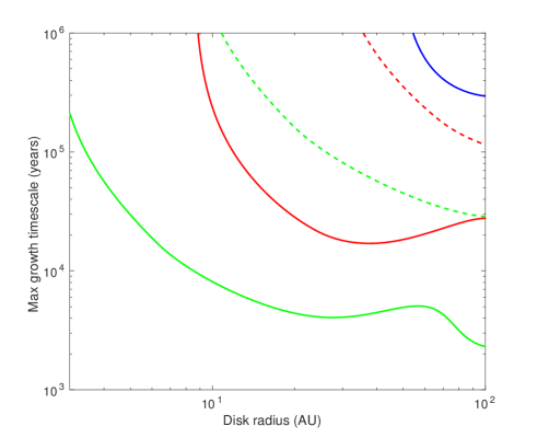
Figure 6: Maximum e-folding times for the SGI at different radii in a standard disk model with $F=1$ and dust-to-gas ratio $\delta=0.01$. The solid curves correspond to cm sized particles, and the dashed curves to mm sized particles. The blue colour represents a turbulent mass diffusivity of $\alpha_{g}=10^{-5}$, red represents $\alpha_{g}=10^{-6}$, and green $\alpha_{g}=10^{-7}$.

We also compute the minimum e-folding times for the SGI, for $F=1$ and $\delta=0.01$. These are plotted in Figure 6. Solid curves correspond to cm sized particles and dashed curves correspond to mm sized particles. We omit smaller particles because they are always in the well-coupled regime treated in Section 6.2. The different colours represent different values of $\alpha_{g}$. As is clear, a turbulence level of $\alpha_{g}>10^{-5}$ yields a growth time too long to be important for both particle classes, while a value of $\alpha_{g}=10^{-6}$ yields a growth time of a few $10^{4}$ years for cm sized particles, at a large range of radii $\gtrsim 20$ AU. Milimetre sized particles exhibit appreciable growth only for low turbulence levels $\alpha_{g}\sim 10^{-7}$ and at larger radii $\gtrsim 50$ AU. Less massive disks (such as with $F=0.1$) yield even weaker growth. Increasing $\delta$ to 0.1, exacerbates growth by up to an order of magnitude, whereas decreasing $F$ to 0.1, reduces the growth rate by roughly an order of magnitude.

These growth times are on the whole consistent with Youdin (2011) at radii $\gtrsim 20$ AU, but closer to the disk two-fluid effects lead to noticeable departures. The growth times diverge at certain critical radii. These occur, of course, when the SGI is stabilised, as indicated by Fig. 5. For a given $\alpha_{g}$, any given particle size has a critical radius within which the SGI is stable. The takeaway message is that mm sized particles require very low levels of turbulence to be SGI unstable, and then this is localised to the outer parts of the disk. Centimetre sized particles do better, and the SGI may play some role in their dynamics across a range of disk radii and disk properties. Finally, older, less massive disks struggle to host the SGI in any form, though a larger dust to gas ratio can mitigate this to some degree. Unfortunately, like $\alpha_{g}$, the parameter $\delta$ is difficult to constrain.

7 Conclusion

In this paper we have explored the secular gravitational instability (SGI) using a simple two-fluid model. Despite the complexity of its associated sixth order dispersion relation, analytic stability criteria and growth rates can be obtained in the two limits of weakly and strongly coupled particles. We find that on sufficiently long and short radial scales the SGI is stabilised; the existence of an unstable range of intermediate scales leads to an explicit instability condition involving the gas’s Toomre parameter, a distinctive feature of the two-fluid SGI, as opposed to the single-fluid version.

The mathematical analysis suggests a straightforward way to understand the instability mechanism. The SGI favours intermediate scales upon which stabilising dust pressure or turbulence is weak, but upon which the gas pressure is strong. The latter condition permits the gas to fall into geostrophic balance: hence when the gas is azimuthally accelerated by the dust drag, it will form a zonal flow rather than undergo epicycles that would disrupt the radially collapsing dust.

An assessment of the prevalence of SGI in real disk models is handicapped by uncertainties in two parameters, the strength of the turbulence $\alpha_{g}$, and the mass ratio of a certain species of dust to the gas within the dust subdisk, $\delta$. Starting with a fiducial value of $\delta=0.01$, we find that a moderate level of turbulence $\alpha_{g}=10^{-5}$ prohibits the SGI on most radii, and when it does occur it grows too slowly $\sim 10^{5}$ years — the timescale of the large-scale evolution of the disk, and of appreciable radial drift. Weaker turbulence $\alpha_{g}=10^{-6}$ permits growth for cm sized particles on radii $\gtrsim 10$ AU, with efolding times of a few $10^{4}$ years. Smaller sized particles may be subject to SGI but grow too slowly. It is only for $\alpha_{g}=10^{-7}$ that mm sized particles sustain growth at reasonable levels, and then only for $R>10$ AU. Increasing $\delta$ improves the situation, of course, and $\delta>0.01$ might be the case for particularly well-settled and populous subclasses of particle, though further work is needed to better constrain this parameter. Even so, if $\alpha_{g}>10^{-6}$ it may be prove difficult for the SGI to meaningfully impose itself on the disk dynamics.

We also discuss the various shortcomings of the razor-thin model we employ, which is especially a problem when the dust and gas disks exhibit different scale thicknesses. These issues no doubt impact quantitatively on our results, but the main qualitative conclusions and our picture of instability should be robust. They can be checked with a suitable vertically stratified analysis akin to Mamatsashvili & Rice (2010) and Lin (2014), which will also provide more reliable quantitative estimates on the stability curves and growth rates.

Our results extend previous analyses of the SGI, and for larger radii are in relative agreement with Youdin (2011) and Shariff & Cuzzi (2011). A notable difference is that the two-fluid model prohibits SGI on radii less than a critical radius. As a result, the SGI is certainly unviable on radii $<1$ AU, and possibly absent on radii $<10$ AU, the expected regions of planet formation. The prospects for SGI in the cm class of particles on disk radii $\sim 10$ AU are reasonable as long as gas turbulence is not too efficient $\alpha_{g}\lesssim 10^{-6}$. The instability could then be an important route by which large aggregates could form further out, leapfrogging the entire range of difficult cm to km sizes. Note that our results are only for axisymmetric instability. It is likely, via analogy with classical GI, that non-axisymmetric SGI occurs for larger $Q_{g}$, in which case our stability curves may need some revision.

It has been hypothesised that the SGI generates observed dust ring structures at larger radii in protoplanetary disks (TI). As discussed in Section 6, however, the SGI has great difficulty on radii $\gtrsim 10$ AU for small particle less than a cm in size. The dust-to-gas ratio $\delta$ needs to be increased, and $Q_{g}$ taken to levels approaching 1 in order to obtain instability. While it may be possible to justify increasing $\delta$, such a low $Q_{g}$ would mean the gas disk is marginally unstable to classical GI. Perhaps a more important point is that, while the linear phase of the SGI evolution is axisymmetric, its nonlinear phase will most likely involve a non-axisymmetric breadown into disordered flow, as in classical GI, not the formation of large-scale quasi-steady rings. Dedicated nonlinear simulations are required to test what dynamics the SGI exhibits once it reaches nonlinear amplitudes, and how readily it forms planetesimal clumps. This forms the basis of future work.

References

- (1) Armitage, P.J., 2010. Astrophysics of Planet Formation, CUP, Cambridge UK.
- (2) Bai, X., 2014. ApJ, 791, 137.
- (3) Binney, J., Tremaine, S., 1987. Galactic dynamics, Princeton Uni. Press.
- (4) Brauer, F., Dullemond, C.P., Henning, Th., 2008. AA, 480, 859.
- (5) Brogan, C.L., and 83 co-authors, 2015. ApJL, 808, L3.
- (6) Carballido et al 2006
- (7) Chiang, E., Youdin, A.N., 2010. AREPS, 38, 493.
- (8) Cuzzi, J.N., Dobrovolskis, A.R., Champney, J.M., 1993. Icarus, 106, 102.
- (9) Cuzzi, J.N., Hogan R.C., Paque, J.M., Dobrovolskis, A.R., 2001. ApJ, 546, 496.
- (10) Davidson, P.A., 2004. Turbulence: An introduction for scientists and engineers, Oxford Uni. Press, Oxford.
- (11) Frisch, U., 1995. Turbulence, Cambridge University Press, Cambridge.
- (12) Garaud, P., Meru, F., Galvagni, M., Olczak, C., 2013. ApJ, 764, 146.
- (13) Goldreich, P., Lynden-Bell, D., 1965. MNRAS, 130, 125.
- (14) Goldreich, P., Tremaine, S., 1978. Icarus, 34, 227.
- (15) Jacquet, E., Balbus, S., Latter, H., 2011. MNRAS, 415, 3591.
- (16) Johansen, A., Blum, J., Tanaka, H., Ormel, C., Bizzarro, M., Rickman, H., 2014. In: Protostars and Planets VI, Beuther, H., Klessen, R.S., Dullemond, C.P., Henning, T. (eds), p537.
- (17) Lesur, G., Kunz, M.W., Fromang, S., 2014. AA, 566, 56.
- (18) Lin, M-K, 2014. ApJ, 790, 13.
- (19) Mamatsashvili, G.R., Rice, W.K.M, 2010. MNRAS, 406, 2050.
- (20) Michikoshi, S., Kokubo, E., Inutsuka, S-I, 2012. ApJ, 746, 35.
- (21) Ogilvie, G.I., 1998. MNRAS, 297, 291.
- (22) Papaloizou, J.C.B., Terquem, C., 2006. RPPh, 69, 119.
- (23) Safronov, V.S., 1969. Evolution of the Protoplanetary Cloud and Formation of the Earth and the Planets. Nauka, Moscow (NASA Technical Translation TTF-677).
- (24) Shariff, K., Cuzzi, J.N., 2011. ApJ, 738, 73.
- (25) Schräpler, R., Henning, T., 2004. ApJ, 614, 960.
- (26) Shadmehri, M., 2016. ApJ, 817, 140.
- (27) Shu, F.H., 1984. In: Planetary Rings, Greenberg, R., Brahic, A. (eds), p513.
- (28) Takahashi, S.Z., Inutsuka, S-I, 2014 (TI). ApJ, 794, 55.
- (29) Takahashi, S.Z., Inutsuka, S-I, 2016. AJ (accepted).
- (30) Turner, N.J., Fromang, S., Gammie, C., Klahr, H., Lesur, G., Wardle, M., Bai, X-N, 2014. In: Protostars and Planets VI, Beuther, H., Klessen, R.S., Dullemond, C.P., Henning, T. (eds), p411.
- (31) Ward, W.R., 2000. In: Origin of the earth and moon, Canup, R.M., Righter, K. (eds), University of Arizona Press, Tucson, p75.
- (32) Windmark, F., Birnstiel, T., Güttler, C., Blum, J., Dullemond, C.P., Henning, Th., 2012a. AA, 540, 73.
- (33) Windmark, F., Birnstiel, T., Ormel, C.W., Dullemond, C.P., 2012b. AA, 544, 16.
- (34) Goldreich, P., Ward, W.R., 1973. ApJ, 183, 1051.
- (35) Youdin, A.N., 2005. arXiv:astro-ph/0508659
- (36) Youdin, A.N., 2011. ApJ, 731, 99.
- (37) Youdin, A.N., Goodman, J., 2005. ApJ, 620, 459.
- (38) Youdin, A.N., Lithwick, Y., 2007. Icarus, 192, 588.
- (39)