The $NLO$ production of the $W^{\pm}$ and $Z^{0}$ vector bosons via hadron collisions in the frameworks of $KMR$ and $MRW$ unintegrated parton distribution functions

Abstract

In a series of papers, we have investigated the compatibility of the $Kimber$-$Martin$-$Ryskin$ ($KMR$) and $Martin$-$Ryskin$-$Watt$ ($MRW$) $unintegrated$ parton distribution functions ($UPDF$) as well as the description of the experimental data on the proton structure functions. The present work is a sequel to that survey, via calculation of the transverse momentum distribution of the electro-weak gauge vector bosons in the $k_{t}$-factorization scheme, by the means of the $KMR$, the $LO\;MRW$ and the $NLO\;MRW$ $UPDF$, in the next-to leading order ($NLO$). To this end, we have calculated and aggregated the invariant amplitudes of the corresponding $involved$ diagrams in the $NLO$, and counted the individual contributions in different frameworks. The preparation process for the $UPDF$ utilizes the $PDF$ of $Martin$ et al, $MSTW2008-LO$, $MSTW2008-NLO$, $MMHT2014-LO$ and $MMHT2014-NLO$ as the inputs. Afterwards, the results have been analyzed against each other, as well as the existing experimental data. Our calculation show excellent agreement with the experiment data. It is however interesting to point-out that, the calculation using the $KMR$ framework illustrates a stronger agreement with the experimental data, despite the fact that the $LO\;MRW$ and the $NLO\;MRW$ formalisms employ a better theoretical description of the $DGLAP$ evolution equation. This is of course due to the use of the different implementation of the angular ordering constraint in the $KMR$ approach, in which automatically includes the re-summation of $ln({1/x})$, $BFKL$ logarithms, in the $LO$-$DGLAP$ evolution equation.

I Introduction

In the recent years, new discoveries have been made at many high energy particle physics laboratories, including the $LHC$, concerning physics within the boundaries of the Standard Model and beyond, as the consequence of pushing the maximum energy of the experiments to the new limits. Today, many of these laboratories use parton distribution functions ($PDF$) to describe and analysis their extracted data from the deep inelastic $QCD$ collisions. These scale-dependent functions are the solutions of the $Dokshitzer$-$Gribov$-$Lipatov$-$Altarelli$-$Parisi$ ($DGLAP$) evolution equations, DGLAP1 ; DGLAP2 ; DGLAP3 ; DGLAP4 ,

$${da(x,Q^{2})\over dlog(Q^{2})}={\alpha_{s}(Q^{2})\over 2\pi}\sum_{b=q,g}\left[\int_{x}^{1}dzP_{ab}(z)b({x\over z},Q^{2})-a(x,Q^{2})\int_{0}^{1}dzzP_{ba}(z)\right],$$ (1)

where $a(x,Q^{2})$ can be either the distribution function of the quarks, $xq(x,Q^{2})$, or that of the gluons, $xg(x,Q^{2})$, with $x$ being the fraction of the longitudinal momentum of the parent hadron (the $Bjorken$ variable). The terms on the right-hand side of the equation (1), correspond to the real emission and the virtual contributions, respectively. The scale $Q^{2}$ is an ultra-violet cutoff, related to the virtuality of the exchanged particle during the deep inelastic scattering ($DIS$). $P_{ab}(z)$ are the splitting functions of the respective partons which account for the probability of emerging a parton $a(x^{\prime\prime},Q^{2})$ from a parent parton $b(x^{\prime},Q^{2})$ through $z=x^{\prime\prime}/x^{\prime}$.

The $DGLAP$ evolution equation however, is based on the $strong\;ordering$ assumption, which systematically neglects the transverse momentum of the emitted partons along the evolution ladder. It has been repeatedly hinted that undermining the contributions coming from the transverse momentum of the partons may severely harm the precision of the calculations, especially in the high energy processes in the small-$x$ region, see for example the references KMR ; MRW ; KKMS ; KIMBER ; WattWZ . This signaled the necessity of introducing some transverse momentum dependent parton distribution functions ($TMD\;PDF$), initially trough the $Ciafaloni$-$Catani$-$Fiorani$-$Marchesini$ ($CCFM$) equation CCFM1 ; CCFM2 ; CCFM3 ; CCFM4 ; CCFM5 ,

$$f(x,k_{t}^{2},Q^{2})=f_{0}(x,k_{t}^{2},Q^{2})+\int^{1}_{x}dz\int{dq^{2}\over q^{2}}\Theta(Q-zq)\Delta_{S}(Q,zq)$$

$$\times P(z,\bar{\alpha}_{s}(k_{t}^{2}))f({x\over z},|\mathbf{k_{t}}+(1-z)\mathbf{q}|^{2},q^{2}).$$ (2)

The $\Theta(Q-zq)$ implies a physical condition, enforcing the increase of the angle of the emission of the gluons in successive radiations along the evolution chain. This condition which is usually referred to as the angular ordering constraint ($AOC$), is due to the coherent radiation of the gluons. The $Sudakov$ form factor, $\Delta_{S}(Q,q)$, gives the probability of evolving from a scale $q$ to a scale $Q$, without any partons emission, and can be defined as:

$$\Delta_{S}(Q,q)=exp\left(-\bar{\alpha_{s}}\int^{Q^{2}}_{q^{2}}{dk^{2}\over k^{2}}\int^{1}_{0}{dz^{\prime}}{1\over(1-z)}\right),$$ (3)

with $\bar{\alpha_{s}}=3\alpha_{s}/\pi$. In the equation (2), $f(x,k_{t}^{2},\mu^{2})$ is the double-scaled $CCFM$ $TMD$ $PDF$, which in addition to the $x$ and $Q$, depends on the transverse momentum of the incoming partons, $k_{t}$. It has been shown (see the reference CCFM-unfolding ) that in the proper boundaries, the $CCFM$ equation will reduced to the conventional $DGLAP$ and $Balitski$-$Fadin$-$Kuraev$-$Lipatov$ ($BFKL$) equations, BFKL1 ; BFKL2 ; BFKL3 ; BFKL4 ; BFKL5 .

The procedure of solving the $CCFM$ equation is mathematically involved and unrealistically time consuming, since it includes contemplating iterative integral equations with many terms. On the other hand, the main feature of the $CCFM$ equation, i.e. the $AOC$, can be exclusively used for the gluon evolution and therefore, this process is incapable of producing convincing quark contribution. To overcome these obstacles, Martin et al have introduced the $k_{t}$-factorization framework and developed the $Kimber$-$Martin$-$Ryskin$ ($KMR$) and the $Martin$-$Ryskin$-$Watt$ ($MRW$) approaches KMR ; MRW , both of which are constructed around the $LO$ $DGLAP$ evolution equations and modified with the different visualizations of the angular ordering constraint. The frameworks of $KMR$ and $MRW$ in the $LO$ and $NLO$ have been investigated intensely in the recent years, see the references Modarres1 ; Modarres2 ; Modarres3 ; Modarres4 ; Modarres5 ; Modarres6 ; Modarres7 ; Modarres8 .

Although $Martin$ et al have developed the $MRW$ formalism as an improvement to the $KMR$ approach, by correcting the use of the $AOC$, limiting its effect only on the diagonal splitting functions and extending the range of their calculations into the $NLO$ via introducing the $NLO\;MRW$ scheme, it appears that the $KMR$ approach, as an effective model, is more successful in producing a realistic theory in order to describe the experiment. We are therefore eager to expand our investigation regarding the merits and shortcomings of these frameworks into the calculation of the inclusive cross-sections of production of the electro-weak gauge bosons in high energy hadronic collisions.

The process of the production of the massive gauge vector bosons, $W^{\pm}$ and $Z^{0}$, have always been of extreme theoretical and experimental interest, since it can provide invaluable information about the nature of both the electro-weak and the strong interactions, setting a benchmark for testing the validity of the experiments and establishing a firm base for testing new theoretical frameworks, see the references UA1 ; UA2 ; CDF96 ; CDF2000 ; D095 ; D098 ; D02000-1 ; D02000-2 ; D02001 ; LIP1 ; Deak1 . It is not however straightforward to describe the transverse momentum distributions of the electro-weak bosons produced in hadron-hadron collisions, since the usual collinear factorization approach in the $LO$, neglects the transverse momentum dependency of the incoming partons and therefore predicts a vanishing transverse momentum for the product. Consequently, initial-state $QCD$ radiation is necessary to generate the $k_{t}$ distributions. On the other hand, in this approximation, calculations for differential cross sections of the $W^{\pm}$ and $Z^{0}$ production diverge logarithmically in the $NLO$ limit for the $k_{t}\ll M_{W,Z}$ (which is the main region of interest), due to the soft gluon emission. So, one requires a re-summation to obtain a finite $k_{t}$ distribution.

In the present work we tend to calculate the $k_{t}$ distributions of the cross-section of production of the $W^{\pm}$ and $Z^{0}$ using the $NLO$ level diagrams and the $LO$ and $NLO$ $UPDF$ of the $KMR$ and the $MRW$ frameworks. The $UPDF$ will be prepared in their proper $k_{t}$-factorization schemes using the $PDF$ of $MSTW2008-LO$, $MSTW2008-NLO$, $MMHT2014-LO$ and $MMHT2014-NLO$, MSTW1 ; MSTW2 ; MSTW3 ; MMHT . Such calculations have been previously carried out using $LO$ matrix elements of quark-antiquark annihilation cross section and doubly-unintegrated parton distribution functions ($DUPDF$) in the framework of $(k_{t},z)$-factorization, reference WattWZ , and in a semi-$NLO$ approach, using a mixture of $LO$ and $NLO$ matrix elements for the involved processes in addition to a variety of $TMD$ $PDF$, see the reference LIP1 . To improve these approximations and at the same time, test the functionality of the $KMR$ and the $MRW$ $UPDF$, we have calculated the $NLO$ ladder diagrams for $g+g\rightarrow W^{\pm}/Z^{0}+q+q^{\prime}$, $q+g\rightarrow W^{\pm}/Z^{0}+q^{\prime}+g$ and $q+q^{\prime}\rightarrow W^{\pm}/Z^{0}+g+g$, utilizing a physical gauge for the gluons. In this way, at the price performing long and complicated calculations, we will demonstrate that with the use of the $UPDF$ in the $NLO$ calculations, one can extract an excellent description of the experimental data of the $D0$ [5,8,9] and $CDF$ [4] collaborations, as well as others works given here, regarding the transverse momentum distributions of the $W^{\pm}$ and $Z^{0}$ boson.

In what follows, first, a brief introduction to the concept of $k_{t}$-factorization will be presented and the respective formalisms for the $KMR$ and the $MRW$ frameworks will be derived, in the section 2. The section 3 contains a comprehensive description over the utilities and means for the calculation of the $k_{t}$-dependent cross-section of production of the $W^{\pm}$ and $Z^{0}$ gauge vector bosons in a hadron-hadron (or hadron-antihadron) deep inelastic collision. The necessary numerical analysis will be presented in the section 4, after which a thoroughgoing conclusion will be followed in the section 5.

II The $k_{t}$-factorization scheme

A parton entering the sub-process at the top of the evolution ladder, has non-negligible transverse momentum. However, it is customary to use the $PDF$ of the $DGLAP$ or the $BFKL$ evolution equations to describe such partons, despite the fact that these density functions intrinsically carry no $k_{t}$-dependency. To include the contributions coming from the transverse momentum distributions of the partons, one can either use the solutions of the $CCFM$ evolution equation or unify the $BFKL$ and the $DGLAP$ evolution equations to form a properly tuned $k_{t}$-dependent framework, unified ; stasto1 . Nevertheless, given the mathematical complexity of these schemes, it is not desirable to use them in the task of computing the $DIS$ cross-sections. Another way is to convolute the single-scaled solutions of the $DGLAP$ evolution equation and insert the required $k_{t}$-dependency via the process of $k_{t}$-factorization (for a complete description see the reference KIMBER ).

Thus, one may define the $UPDF$, $f_{a}(x,k_{t}^{2},\mu^{2})$, in the $k_{t}$-factorization scheme, through the following normalization relation,

$$a(x,\mu^{2})=\int^{\mu^{2}}{dk_{t}^{2}\over k_{t}^{2}}f_{a}(x,k_{t}^{2},\mu^{2}),$$ (4)

where $a(x,\mu^{2})$ are the solutions of the $DGLAP$ equation and stand for either $xq(x,\mu^{2})$ or $xg(x,\mu^{2})$. The procedure of deriving a direct expansion for $f_{a}(x,k_{t}^{2},\mu^{2})$, in terms of the $PDF$ is strait forward. Yet, exposing the resulting prescriptions to the different visualizations of the $AOC$ will produce different $UPDF$, namely the $KMR$, the $LO\;MRW$ and the $NLO\;MRW$ frameworks. In what follows, we will describe these frameworks in detail.

II.1 The $KMR$ framework

Starting form the $DGLAP$ equation in the leading order, the equation (1), and using the unregulated $LO$ $DGLAP$ splitting kernels, $P_{ab}(z)$, the reference WATT , $Kimber$ et al introduced an infrared cut-off, $\Delta$, as a visualization of the $AOC$ KMR1 ,

$$\Theta(\theta-\theta^{\prime})\Longrightarrow\mu>{zk_{t}\over(1-z)}\Longrightarrow\Delta={k_{t}\over\mu+k_{t}}.$$

Limiting the upper boundary on $z$ integration by $\Delta$, excludes $z=1$ form the integral equation and automatically prevents facing the soft gluon singularities arising form the $1/(1-z)$ terms in the splitting functions. Additionally, they factorized the virtual contributions from the $DGLAP$ equations, by defining a virtual (loop) contributions as:

$$T_{a}(k_{t}^{2},\mu^{2})=exp\left(-\int_{k_{t}^{2}}^{\mu^{2}}{\alpha_{S}(k^{2})\over 2\pi}{dk^{2}\over k^{2}}\sum_{b=q,g}\int^{1-\Delta}_{0}dz^{\prime}P_{ab}^{(LO)}(z^{\prime})\right),$$ (5)

with

$$T_{a}(\mu^{2},\mu^{2})=1,$$

as an appropriated form of the $Sudakov$ form factor, the equation (3). Afterwards, the double-scaled $KMR$ $UPDF$ are defined as follows:

$$f_{a}(x,k_{t}^{2},\mu^{2})=T_{a}(k_{t}^{2},\mu^{2})\sum_{b=q,g}\left[{\alpha_{S}(k_{t}^{2})\over 2\pi}\int^{1-\Delta}_{x}dzP_{ab}^{(LO)}(z)b\left({x\over z},k_{t}^{2}\right)\right].$$ (6)

According to the above formulation, only at the last step of the evolution, the dependence on the second scale, $\mu$, gets introduced into the $UPDF$. The required $PDF$ is provided as input, using the libraries $MSTW2008$ MSTW1 ; MSTW2 ; MSTW3 and $MMHT2014$ MMHT , where the calculation of the single-scaled functions have been carried out using the $DIS$ data on the $F_{2}$ structure function of the proton. $T_{a}$ are considered to be unity for $k_{t}>\mu$. This constraint and its interpretation in terms of the strong ordering condition gives the $KMR$ approach a smooth behavior over the small-$x$ region, which is generally governed by the $BFKL$ evolution equation.

II.2 The $LO\;MRW$ framework

In coordination with the theory of gluonic coherent radiation, it has been pointed out that the $AOC$ in the $KMR$ formalism should only act on the terms including the on-shell gluon emissions, i.e. the diagonal splitting functions $P_{qq}(z)$ and $P_{gg}(z)$. Therefore, $Martin$ et al defined the $LO$ $MRW$ $UPDF$ as the correction to the $KMR$ framework MRW ,

$$f_{q}^{LO}(x,k_{t}^{2},\mu^{2})=T_{q}(k_{t}^{2},\mu^{2}){\alpha_{S}(k_{t}^{2})\over 2\pi}\int_{x}^{1}dz\left[P_{qq}^{(LO)}(z){x\over z}q\left({x\over z},k_{t}^{2}\right)\Theta\left({\mu\over\mu+k_{t}}-z\right)\right.$$

$$\left.+P_{qg}^{(LO)}(z){x\over z}g\left({x\over z},k_{t}^{2}\right)\right],$$ (7)

with

$$T_{q}(k_{t}^{2},\mu^{2})=exp\left(-\int_{k_{t}^{2}}^{\mu^{2}}{\alpha_{S}(k^{2})\over 2\pi}{dk^{2}\over k^{2}}\int^{z_{max}}_{0}dz^{\prime}P_{qq}^{(LO)}(z^{\prime})\right),$$ (8)

for the quarks and

$$f_{g}^{LO}(x,k_{t}^{2},\mu^{2})=T_{g}(k_{t}^{2},\mu^{2}){\alpha_{S}(k_{t}^{2})\over 2\pi}\int_{x}^{1}dz\left[P_{gq}^{(LO)}(z)\sum_{q}{x\over z}q\left({x\over z},k_{t}^{2}\right)\right.$$

$$\left.+P_{gg}^{(LO)}(z){x\over z}g\left({x\over z},k_{t}^{2}\right)\Theta\left({\mu\over\mu+k_{t}}-z\right)\right],$$ (9)

with

$$T_{g}(k_{t}^{2},\mu^{2})=exp\left(-\int_{k_{t}^{2}}^{\mu^{2}}{\alpha_{S}(k^{2})\over 2\pi}{dk^{2}\over k^{2}}\left[\int^{z_{max}}_{z_{min}}dz^{\prime}z^{\prime}P_{qq}^{(LO)}(z^{\prime})+n_{f}\int^{1}_{0}dz^{\prime}P_{qg}^{(LO)}(z^{\prime})\right]\right),$$ (10)

for the gluons. In the equations (8) and (10), $z_{max}=1-z_{min}=\mu/(\mu+k_{t})$ WATT . The $UPDF$ of $KMR$ and $MRW$ to a good approximation, include the main kinematical effects involved in the $DIS$ processes. One should note that the particular form of the $AOC$ in the $KMR$ formalism despite being of the $LO$, includes some contributions from the $NLO$ sector, whence in the case of $MRW$ framework, these contributions must be inserted separately.

II.3 The $NLO\;MRW$ framework

The expansions of the $LO$ $MRW$ formalism into the $NLO$ region can be achieved through the following definitions:

$$f_{a}^{NLO}(x,k_{t}^{2},\mu^{2})=\int_{x}^{1}dzT_{a}\left(k^{2}={k_{t}^{2}\over(1-z)},\mu^{2}\right){\alpha_{S}(k^{2})\over 2\pi}\sum_{b=q,g}\tilde{P}_{ab}^{(LO+NLO)}(z)$$

$$\times b^{NLO}\left({x\over z},k^{2}\right)\Theta\left(1-z-{k_{t}^{2}\over\mu^{2}}\right),$$ (11)

with the $NLO$ splitting functions being defined as,

$$\tilde{P}_{ab}^{(LO+NLO)}(z)=\tilde{P}_{ab}^{(LO)}(z)+{\alpha_{S}\over 2\pi}\tilde{P}_{ab}^{(NLO)}(z),$$ (12)

and

$$\tilde{P}_{ab}^{(i)}(z)=P_{ab}^{i}(z)-\Theta(z-(1-\Delta))\delta_{ab}F^{i}_{ab}P_{ab}(z),$$ (13)

where $i=0,1$ stand for $LO$ and $NLO$ respectively. The reader can find a comprehensive description of the $NLO$ splitting functions in the references MRW ; PNLO . We must however emphasis that contrary to the $KMR$ and the $LO$ $MRW$ frameworks, the $AOC$ is being introduced into the $NLO$ $MRW$ formalism via the $\Theta(z-(1-\Delta))$ constraint, in the ”extended” splitting function. Now $\Delta$ can be defined as:

$$\Delta={k\sqrt{1-z}\over k\sqrt{1-z}+\mu}.$$

The $NLO$ corrections introduced into this framework are the collection of the $NLO$ $PDF$, the $NLO$ splitting functions and the constraint $\Theta\left(1-z-{k_{t}^{2}/\mu^{2}}\right)$. Nevertheless, it has been shown that using only the $LO$ part of the extended splitting function, instead of the complete definition of equation (12), would result in reasonable accuracy in computation of the $NLO$ $MRW$ $UPDF$ MRW . Additionally, the $Sudakov$ form factors in this framework are defined as:

$$T_{q}(k^{2},\mu^{2})=exp\left(-\int_{k^{2}}^{\mu^{2}}{\alpha_{S}(q^{2})\over 2\pi}{dq^{2}\over q^{2}}\int^{1}_{0}dz^{\prime}z^{\prime}\left[\tilde{P}_{qq}^{(0+1)}(z^{\prime})+\tilde{P}_{gq}^{(0+1)}(z^{\prime})\right]\right),$$ (14)

$$T_{g}(k^{2},\mu^{2})=exp\left(-\int_{k^{2}}^{\mu^{2}}{\alpha_{S}(q^{2})\over 2\pi}{dq^{2}\over q^{2}}\int^{1}_{0}dz^{\prime}z^{\prime}\left[\tilde{P}_{gg}^{(0+1)}(z^{\prime})+2n_{f}\tilde{P}_{qg}^{(0+1)}(z^{\prime})\right]\right).$$ (15)

Each of these $UPDF$, the $KMR$, $LO$ and $NLO$ $MRW$ can be used to identify the probability of finding a parton of a given flavor, with the fraction $x$ of longitudinal momentum of the parent hadron, the transverse momentum $k_{t}$ in the scale $\mu$ at the semi-hard level of a particular $DIS$ process. In the following section, we will describe the cross-section of the production of the $W^{\pm}$ and $Z^{0}$ bosons with the help of our $UPDF$.

III Production of $W^{\pm}$ and $Z^{0}$ in the $k_{t}$-factorization

By definition, the total cross-section for a deep hadronic collision, $\sigma_{Hadron-Hadron}$, can be written in terms of its possible partonic constituents. Utilizing the $UPDF$ as density functions for the involved partons, one may write $\sigma_{Hadron-Hadron}$ in the following form:

$$\sigma_{Hadron-Hadron}=\sum_{a_{1},a_{2}=q,g}\int_{0}^{1}{dx_{1}\over x_{1}}\int_{0}^{1}{dx_{2}\over x_{2}}\int_{0}^{\infty}{dk^{2}_{1,t}\over k^{2}_{1,t}}\int_{0}^{\infty}{dk^{2}_{2,t}\over k^{2}_{2,t}}f_{a_{1}}(x_{1},k^{2}_{1,t},\mu_{1}^{2})f_{a_{2}}(x_{2},k^{2}_{2,t},\mu_{2}^{2})$$

$$\times\hat{\sigma}_{a_{1}a_{2}}(x_{1},k^{2}_{1,t},\mu_{1}^{2};x_{2},k^{2}_{2,t},\mu_{2}^{2}),$$ (16)

where $a_{1}$ and $a_{2}$ are the incoming partons into the semi-hard process from the first and the second hadrons, respectively. $\hat{\sigma}_{a_{1}a_{2}}$ are the corresponding partonic cross-sections which can be defined separately as,

$$d\hat{\sigma}_{a_{1}a_{2}}={d\phi_{a_{1}a_{2}}\over F_{a_{1}a_{2}}}|{\mathcal{M}_{a_{1}a_{2}}}|^{2}.$$ (17)

$d\phi_{a_{1}a_{2}}$ and $F_{a_{1}a_{2}}$ are the multi-particle phase space and the flux factor, respectively and can be defined according to the specifications of the partonic process,

$$d\phi_{a_{1}a_{2}}=\prod_{i}{d^{3}p_{i}\over 2E_{i}}\delta^{(4)}\left(\sum p_{in}-\sum p_{out}\right),$$ (18)

$$F_{a_{1}a_{2}}=x_{1}x_{2}s,$$ (19)

with the $s$ being the center of mass energy squared.

$$s=(P_{1}+P_{2})^{2}=2P_{1}.P_{2}.$$

$P_{1}$ and $P_{2}$ are the 4-momenta of the incoming protons and since we are working in the infinite momentum frame, it is safe to neglect their masses. $d\phi_{a_{1}a_{2}}$ can be characterized in terms of transverse momenta of the product particles, $p_{i,t}$, their rapidities, $y_{i}$, and the azimuthal angles of the emissions, $\varphi_{i}$,

$${d^{3}p_{i}\over 2E_{i}}={\pi\over 2}dp_{i,t}^{2}dy_{i}{d\varphi_{i}\over 2\pi}.$$ (20)

In the equation (17), ${\mathcal{M}_{a_{1}a_{2}}}$ are the matrix elements of the partonic diagrams which are involved in the production of the final results. To calculate these quantities, one must first understand the exact kinematics that rule over the corresponding partonic processes.

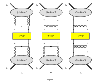
Figure 1: The NLO ladder-type diagrams for the production of $W^{\pm}$ and $Z^{0}$ in the $k_{t}$-factorization framework. The $f_{g}(x,k_{t}^{2},\mu^{2})$ and $f_{q}(x,k_{t}^{2},\mu^{2})$ represent the corresponding UPDF in the KMR, the LO-MRW or the NLO-MRW frameworks, i.e. the equations (6), (7), (9) and (11).

The figure 1 illustrates the ladder-type $NLO$ diagrams that one have to consider, counting the contributions coming from $g+g\rightarrow W^{\pm}/Z^{0}+q+q^{\prime}$, $q+g\rightarrow W^{\pm}/Z^{0}+q^{\prime}+g$, and $q+q^{\prime}\rightarrow W^{\pm}/Z^{0}+g+g$ as shown in the figure 1, panels (a), (b) and (c), respectively. The kinematics and calculations of this type of invariant amplitudes have been discussed extensively in the references WattWZ ; LIP1 ; Deak1 . We have followed the same approach, obtaining the $dk_{i,t}^{2}/k_{i,t}^{2}$ terms only from the ladder-type diagrams, and not from the interference (i.e. the non-ladder) diagrams, using a physical gauge for the gluons, where only the two transverse polarizations propagate,

$$d_{\mu\nu}(k)=-g_{\mu\nu}+{k_{\mu}n_{\nu}+n_{\mu}k_{\nu}\over k.n}.$$ (21)

$n=x_{1}P_{1}+x_{2}P_{2}$ is the gauge-fixing vector. Choosing such a gauge condition, ensures that the $dk_{i,t}^{2}/k_{i,t}^{2}$ terms are being obtained from the ladder-type diagrams on both sides of the sub-processes. In the case of hadron-hadron collisions, one might expect that neglecting the contributions coming from the non-ladder diagrams, i.e. the diagrams where the production of the electro-weak bosons is a by-product of the hadronic collision (see the reference Deak1 ), would have a numerical effect on the results. Nevertheless, employing the gauge choice (21), one finds out that the contribution from the ”unfactorizable” non-ladder diagrams vanishes.

In the proton-antiproton center of mass frame, we can write the following kinematics

$$P_{1}={\sqrt{s}\over 2}(1,0,0,1),\;\;\;P_{2}={\sqrt{s}\over 2}(1,0,0,-1),$$

$$\textbf{k}_{i}=x_{i}\textbf{P}_{i}+\textbf{k}_{i,\perp},\;\;\;k_{i,\perp}^{2}=-k_{i,t}^{2},\;\;\;i=1,2\;,$$ (22)

where the $k_{i},\;i=1,2$ are the 4-momenta of the partons that enter the semi-hard process. Afterwards, it is possible to write the law of the transverse momentum conservation for the partonic process:

$$\textbf{k}_{1,\perp}+\textbf{k}_{2,\perp}=\textbf{p}_{1,\perp}+\textbf{p}_{2,\perp}+\textbf{p}_{\perp},$$ (23)

with $\textbf{p}_{\perp}$ being the transverse momentum of the produced vector boson. Additionally, defining the transverse mass of the produced virtual partons, $m_{i,t}=\sqrt{m^{2}_{i}+p_{i}^{2}}$, we can write,

$$x_{1}=\left(m_{1,t}e^{y_{1}}+m_{2,t}e^{y_{2}}+m_{W/Z,t}e^{y_{W/Z}}\right)/\sqrt{s},$$

$$x_{2}=\left(m_{1,t}e^{-y_{1}}+m_{2,t}e^{-y_{2}}+m_{W/Z,t}e^{-y_{W/Z}}\right)/\sqrt{s}.$$ (24)

Now, using the above equations, one can derive the following equation for the total cross-section of the production of the $W^{\pm}$ and $Z^{0}$ bosons in the framework of $k_{t}$-factorization,

$$\sigma(P+\bar{P}\rightarrow W^{\pm}/Z^{0}+X)=\sum_{a_{i},b_{i}=q,g}\int{dk_{a_{1},t}^{2}\over k_{a_{1},t}^{2}}\;{dk_{a_{2},t}^{2}\over k_{a_{2},t}^{2}}\;dp_{b_{1},t}^{2}\;dp_{b_{2},t}^{2}\;dy_{1}\;dy_{2}\;dy_{W/Z}\;\times$$

$${d\varphi_{a_{1}}\over 2\pi}\;{d\varphi_{a_{2}}\over 2\pi}\;{d\varphi_{b_{1}}\over 2\pi}\;{d\varphi_{b_{2}}\over 2\pi}\times$$

$${|\mathcal{M}(a_{1}+a_{2}\rightarrow W^{\pm}/Z^{0}+b_{1}+b_{2})|^{2}\over 256\pi^{3}(x_{1}x_{2}s)^{2}}\;f_{a_{1}}(x_{1},k_{a_{1},t}^{2},\mu^{2})\;f_{a_{2}}(x_{2},k_{a_{2},t}^{2},\mu^{2}).$$ (25)

Note that the integration boundaries for ${dk_{i,t}^{2}/k_{i,t}^{2}}$ are $(0,\infty)$. One may introduce an upper limit for these, say $k_{i,max}$, several times larger than the scale $\mu$, without any noticeable consequences. Yet, for $k_{t}<\mu_{0}$ with $\mu_{0}=1\;GeV$, i.e. for the non-perturbative region, it is impervious to decide how to validate our $UPDF$. A natural choice would be to fulfill the requirement that

$$\lim_{k_{a_{i},t}^{2}\rightarrow 0}f_{a_{i}}(x_{i},k_{a_{i},t}^{2},\mu^{2})\sim k_{a_{i},t}^{2},$$

and therefore, we can safely choose the following approximation for the non-perturbative region:

$$f_{a_{i}}(x_{i},k_{a_{i},t}^{2}<\mu_{0}^{2},\mu^{2})={k_{a_{i},t}^{2}\over\mu_{0}^{2}}a_{i}(x_{i},\mu_{0}^{2})T_{a_{i}}(\mu_{0}^{2},\mu^{2}).$$ (26)

In the next section, we will introduce some of the numerical methods that have been used for the calculation of the $\sigma(P+\bar{P}\rightarrow W^{\pm}/Z^{0}+X)$, the equation (25), using the $UPDF$ of $KMR$ and $MRW$. It it expected that through considering $NLO$ processes for this computation, the results will have a better agreement with the existing experimental data, in comparison with the previous calculations.

IV Numerical analysis

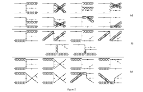
Figure 2: The individual contributions into the matrix elements of the partonic scattering. The diagrams in the panel (a) correspond to the $q+\bar{q}^{\prime}\rightarrow W^{\pm}/Z^{0}+g+g$ sub-process, panel (b) to the $q+g\rightarrow W^{\pm}/Z^{0}+q+g$ sub-process and panel (c) to the $g+g\rightarrow W^{\pm}/Z^{0}+q+\bar{q}^{\prime}$ sub-process. It should be pointed out that one may find additional non-ladder-type diagrams which contribute to these matrix elements. We have eliminated these un-desirable contributions using our choice of the gluon gauge, the equation (21).

The main challenge one must face, in the computions of the total cross-section of a hadron-hadron collision in the $NLO$, is the extremely complex calculations required for extracting the invariant amplitudes in a set of $2\rightarrow 3$ $NLO$ Feynman diagrams. Each of our processes, $g+g\rightarrow W^{\pm}/Z^{0}+q+q^{\prime}$, $q+g\rightarrow W^{\pm}/Z^{0}+q^{\prime}+g$, and $q+q^{\prime}\rightarrow W^{\pm}/Z^{0}+g+g$, include a number of different configurations, see the figure 2. This is when we filter out the non-ladder diagrams, with our choice of the gauge condition on the gluon polarization, the equation (21). Writing the analytic expressions of the $\mathcal{M}_{ab}$ for theses diagrams is rather straight forward, see the Appendix A.

However, since the incoming and the out-going quarks are off-shell, and we do not neglect their transverse momenta, their on-shell spin density matrices has to be replaced with a more complicated expression. To do this, one can extend the original expressions, according to an approximation proposed in the references LIP2 ; LIP3 , through converting the off-shell quark lines to the internal lines via replacing the spinorial elements of the incoming and the out-going partons. Following this idea, we replace the incoming proton with a quark with the momentum $p$ and the mass $m$ which radiates a photon or a gluon and turns into an off-shell quark with the momentum $k$. Therefore, the corresponding matrix element for such quarks can be written as,

$$|\mathcal{M}|^{2}\sim Tr\left(\Gamma_{\mu}\;{\hat{k}+m\over k^{2}-m^{2}}\;\gamma^{\nu}\;u(p)\;\bar{u}(p)\;\gamma_{\nu}\;{\hat{k}+m\over k^{2}-m^{2}}\;\Gamma^{\mu}\right)$$

where $\Gamma_{\mu}$ represents the rest of the original matrix element. Now, the expression presented between $\Gamma_{\mu}$ and $\Gamma^{\mu}$ is considered to be the off-shell quark spin density matrix. Using the on-shell identity

$$\sum u(p)\bar{u}(p)=\hat{p}+m,$$

and after performing some Dirac algebra at the $m\to 0$ limit, one simply arrives to the following expression:

$$|\mathcal{M}|^{2}\sim{2\over k^{4}}Tr\left(\Gamma_{\mu}\;\left[k^{2}\hat{p}-2(p\cdot k)\hat{k}\right]\;\Gamma^{\mu}\right).$$

Afterwards, imposing the Sudakov decomposition $k=xp+k_{t}$ with $k^{2}=k^{2}_{t}=-\textbf{k}^{2}_{t}$, one derives:

$$|\mathcal{M}|^{2}\sim{2\over xk^{2}_{t}}\;Tr\left(\Gamma_{\mu}\;x\hat{p}\;\Gamma^{\mu}\right).$$ (27)

Thus, with the above replacement, the negative light-cone momentum fractions of the incoming partons have been neglected. $x\hat{p}$ in this equation represents the properly normalized off-shell spin density matrix. Additionally, the coupling vertices of the off-shell gluons to quarks must be modified with the eikonal vertex (i.e the $BFKL$ prescription, see the reference Deak1 ). Therefore, in the case of initial off-shell gluons, we impose the so-called non-sense polarization condition, i.e.

$$\epsilon_{\mu}(k_{i})={2k_{i,\mu}\over\sqrt{s}},$$

which results into the following normalization identity

$$\sum\epsilon_{\mu}(k_{i})\epsilon_{\nu}^{*}(k_{i})={k_{i,\mu}k_{i,\nu}\over k_{i,t}^{2}}.$$

We can calculate the evolution of the traces of the matrix elements with the help of the algebraic manipulation system $\mathtt{FORM}$, FORM . Also, the method of orthogonal amplitudes, see the reference Deak1 , can be used to further simplify the results.

The numerical computation of the equation (25) have been carried out using the $\mathtt{VEGAS}$ algorithm in the Monte-Carlo integration. To do this, we have selected the hard-scale of the $UPDF$ to be equal to the transverse mass of the produced gauge vector boson:

$$\mu=(m_{W/Z}^{2}+p_{W/Z,t}^{2})^{1\over 2}.$$

Mathematically speaking, the upper bound on the transverse momentum integrations of the master equation (25) should be the infinity. However, since the $UPDF$ of $KMR$ and $MRW$ tend to quickly vanish in the $k_{t}\gg\mu$ domain, one can safely introduce an ultraviolet cut-off for these integrations. By convention, this cut-off is considered to be at $k_{i,max}=p_{i,max}=4\mu$. Nevertheless, given that $\mu$ depends on the transverse momentum of the produced boson ($p_{W/Z,t}$) and its mass, it would be sufficient to set $k_{i,max}=p_{i,max}=4\mu_{max}$, with

$$\mu_{max}=(m_{W/Z}^{2}+p_{t,max}^{2})^{1\over 2}.$$

One can easily confirm that further domain have no contribution into our results. Also it is satisfactory to bound the rapidity integrations to $[-10,10]$, since $0\leq x\leq 1$ and according to the equation (24), further domain has no contribution into our results. The choice of above hard scale is reasonable for the production of W and Z bosons, as has been discussed in the reference Deak1 .

As a final note, we should make it clear that in the reference LIP1 , the calculation of the transverse momentum distribution for the production of the $W$ and $Z$ bosons has been carried out, using the aggregated contributions of the following sub-processes:

• The $NLO$ $g+g\to W/Z+q+\bar{q}$ partonic process, using the unintegrated gluon distributions of the $CCFM$ and the $LO$ $MRW$ formalisms, accounting for the production of the bosons accompanied by (at least) two distinct jets.

• The $LO$ $q+g\to W/Z+\bar{q}$ partonic process, with the density function of the incoming quarks and gluons being defined in the collinear ($GRV$ or $MSTW$) and the $k_{t}$-factorization (the $CCFM$ and the $LO$ $MRW$) formalisms, respectively. This corresponds to the $p+\bar{p}\to W/Z+jet+X$ cross-section.

• The $LO$ $q+\bar{q}\to W/Z$ partonic process, from the collinear approximation, assuming that the incoming particles are valance quarks (or valance anti-quarks).

The above paratonic processes (a, b and c) obviously neglect some of the $NLO$ contributions (in the b and c cases), namely the shares of the non-valance quarks along the chain of evolution. Additionally, assuming the non-zero transverse momentum for the valance quarks in the infinite momentum frame is to some extent unacceptable, since, in the absence of any extra structure, the intrinsic transverse momenta of the valance quarks should not be enough for producing the $W/Z$ bosons with relatively large $p_{t}$. In the present work, we have upgraded the partonic processes of the b and c cases with their NLO counterparts, i.e. $q^{*}+g^{*}\to W/Z+q+g$ and $q^{*}+\bar{q}^{*}\to W/Z+g+g$ sub-processes. So, we are able to use the UPDF of the $k_{t}$-factorization for the incoming quarks and gluons to insert the transverse momentum dependency of the produced bosons, and at the same time avoid over-counting. Furthermore, the problem of separating the $W/Z$+single-jet and the $W/Z$+double-jet cross-sections will reduce to inserting the correct physical constraints on the dynamics of these processes, e.g. via inserting some transverse momentum cuts for the produced jets, using the anti-$k_{t}$ algorithm, see the reference anti-kt . Nevertheless, since we are interested to calculate the inclusive cross-section for the production of the $W/Z$ bosons, inserting such constraints is unnecessary.

V Results, Discussions and Conclusions

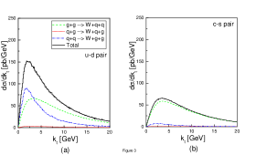
Figure 3: The differential cross-section of the productions of $W^{\pm}$ bosons in a DIS at $E_{CM}=1.8\;TeV$, against the transverse momentum distribution of the produced particle. The panels (a) and (b) illustrate the up-down and charm-strange contributions, respectively. The contribution of each partonic sub-process is singled out: the green-dash histogram is for $g+g\rightarrow W^{\pm}+q+\bar{q}^{\prime}$, the red-dotted histogram is for $q+g\rightarrow W^{\pm}+q^{\prime}+g$ and the blue-dash-dotted histogram is for $q+\bar{q}^{\prime}\rightarrow W^{\pm}+g+g$. The black-full histogram is the total contribution of the give quark pairs. The histograms are produced using the $KMR$ $UPDF$ with the $PDF$ of $MSTW2008$.

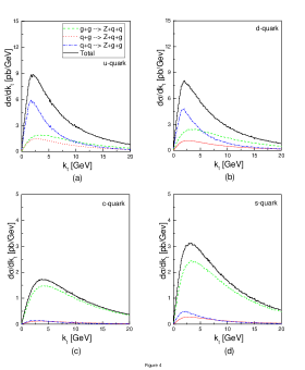
Figure 4: The differential cross-section of the productions of $Z^{0}$ boson in a DIS at $E_{CM}=1.8\;TeV$, against the transverse momentum distribution of the produced particle. The contributions of the up and the down quarks (the panels (a) and (b), respectively) and the lightest sea-quarks (the panel (c) for the charm quark and the panel (d) for the strange quark). The green-dash histogram is for $g+g\rightarrow Z^{0}+q+\bar{q}$, the red-dotted histogram is for $q+g\rightarrow Z^{0}+q+g$ and the blue-dash-dotted histogram is for $q+\bar{q}\rightarrow Z^{0}+g+g$. The black-full histogram is the total contribution of the given quark. The data is produced using the $KMR$ $UPDF$, with the $PDF$ of $MSTW2008$.

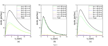
Figure 5: The contributions of the individual partonic sub-processes into the differential cross-section of the productions of $W^{\pm}$ bosons in a DIS at $E_{CM}=1.8\;TeV$, versus the transverse momentum distribution of the produced particle. The panels (a), (b) and (c) correspond to the $g+g\rightarrow W^{\pm}+q+\bar{q}^{\prime}$, $q+\bar{q}^{\prime}\rightarrow W^{\pm}+g+g$ and $g+q\rightarrow W^{\pm}+g+q^{\prime}$ sub-processes, respectively. The data have been obtained using the $UPDF$ of $KMR$, with the $PDF$ of $MSTW2008$.

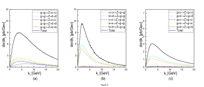
Figure 6: The contributions of the individual partonic sub-processes into the differential cross-section of the productions of $Z^{0}$ bosons in a DIS at $E_{CM}=1.8\;TeV$, versus the transverse momentum distribution of the produced particle. The notions of the diagrams are the same as in the figure 5.

Using the theory and the notions of the previous sections, one can calculate the production rate of the $W^{\pm}$ and $Z^{0}$ gauge vector bosons for the center-of-mass energy of $1.8$ $TeV$. The $PDF$ of Martin et al MSTW1 ; MSTW2 ; MSTW3 ; MMHT , $MSTW2008$ and $MMHT2014$, are used as the input functions to feed the equations (6), (7), (9) and (11). The results are the double-scale $UPDF$ in the $KMR$, the $LO\;MRW$ and the $NLO\;MRW$ schemes. These $UPDF$ are in turn substituted into the equation (25) to construct the $W/Z$ cross-sections in their respective frameworks. Since we intend to compare our calculations to the $W^{\pm}\to l^{\pm}+\nu$ and $Z\to l^{+}+l^{-}$ decays, we should multiply our theoretical out-put by the relevant branching fractions, i.e. $f(W^{\pm}\to l^{\pm}+\nu)=0.1075$ and $f(Z\to l^{+}+l^{-})=0.03366$ Yao . Thus, the figures 3 and 4 present the reader, with a comparison between the different contributions into the differential cross-sections of the $W^{\pm}$ and $Z^{0}$, versus their transverse momentum ($k_{t}$) in the $KMR$ scheme. The main contributions into the production of the $W^{\pm}$ are those involving $u\to W+d$ and $c\to W+s$ vertices. Other production vertices have been calculated and proven to be negligible compared to these main contributions (nevertheless, for the sake of completeness, we have included every single share, no matter how small they are in the total contributions, see the figures 5 and 6, where the individual contributions of each of the production vertices in the partonic sub-processes for the production of $W^{\pm}$ and $Z^{0}$ have been depicted clearly, in the framework of $KMR$ for $E_{CM}=1.8\;TeV$). In the case of $Z^{0}$ production, the main vertices are $u\to Z+u$, $d\to Z+d$, $c\to Z+c$ and $s\to Z+s$. In both cases, one can recognize the different behavior of various partonic sub-processes. As expected, the contributions of the $g+g\to W/Z+q+\bar{q}^{\prime}$ in all of the diagrams are similar, and even (roughly) of the same size, since they only depend on the behavior of the gluon density. On the other hand, the contribution coming from the $q+\bar{q}^{\prime}\to W/Z+g+g$ differs from one production vertex to another, mimicking the differences between the quark densities of different flavors and going from the high contributions of the up and down quarks to small contributions of the charm and strange and even negligible contributions of the top and bottom quarks. Additionally, one notices the smallness of the $q+g\to W/Z+q^{\prime}+g$ contributions. This is also anticipated, since the incoming gluon could (with a relatively large probability) decay into a quark-antiquark pair that does not have the right flavor to form a production vertex with considerable contribution.

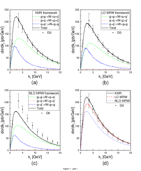
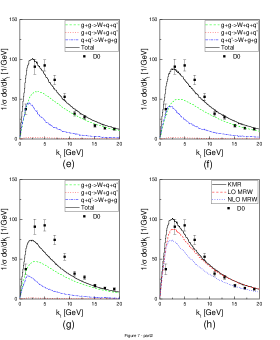
Figure 7: The comparison of the differential cross-section of the $W^{\pm}$ production in the $NLO$ in the $KMR$ (the panel (a)), $LO\;MRW$ (the panel (b)) and $NLO\;MRW$ (the panel (c)) frameworks. The panel (d) illustrates this comparison with the help of experimental data of $D0$ collaboration, the reference D02001 . The panels (e),(f) and (g) are the same values, but this time they deviled by the total cross-sections in their respective framework and compared to an older set of data points from the $D0$ collaboration, D098 . Again, an overall comparison with the experiment is presented in the panel (h). To perform these calculations, we have utilized the $PDF$ of $MSTW2008$.

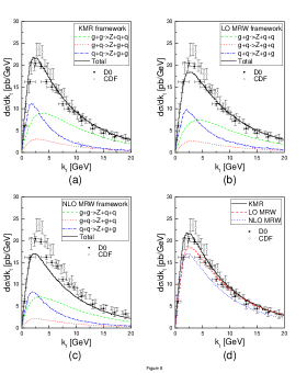
Figure 8: The comparison of the differential cross-section of the $Z^{0}$ production in the $NLO$ in the $KMR$ (the panel (a)), $LO\;MRW$ (the panel (b)) and $NLO\;MRW$ (the panel (c)) frameworks. The panel (d) illustrates this comparison with the help of the experimental data of $D0$ and $CDF$ collaborations, the references D098 ; CDF2000 .

The figures 7 and 8 illustrate a complete comparison between the results of the calculation of the production of the electro-weak gauge vector bosons in the frameworks of $KMR$, $LO\;MRW$ and $NLO\;MRW$, with each other and with the experimental data of the $D0$ and $CDF$ collaborations, references CDF96 ; CDF2000 ; D098 ; D02000-1 ; D02000-2 ; D02001 . The results in the $KMR$ framework has an excellent agreement with the experimental data, both in the $W^{\pm}$ and $Z^{0}$ productions. The $LO\;MRW$ scheme behaves similarly compared to the $KMR$ framework, yet has a noticeably shorter peak, specially in the case of $Z^{0}$. This is due the different visualization of the $AOC$ between these two frameworks, see the section 3. Meanwhile, the results in the $NLO\;MRW$ scheme are unexpectedly unable to describe the experiment data. This is related to the conditions in which the $AOC$ has been imposed in this framework. The $\theta(1-z-{k_{t}^{2}/\mu^{2}})$ constraint gives the parton distributions of the $NLO\;MRW$, a sharp descend to zero at $k_{t}\to\mu$ and returns a vanishing contribution for the better part of the transverse momentum integration in the equation (25). Consequently, the overall value of the differential cross-sections of the $W^{\pm}$ and $Z^{0}$ production in this framework reduces dramatically, as it is apparent in the figures 7 and 8 . In overall and as it has been stated elsewhere (see for example the references Modarres7 ; Modarres8 ) the results in the $KMR$ scheme seemingly have a better agreement with the experiment. This is to some extend ironic, since the $LO$ and the $NLO\;MRW$ formalisms are developed as extensions and improvements to the $KMR$ approach and are more compatible with the $DGLAP$ evolution equation.

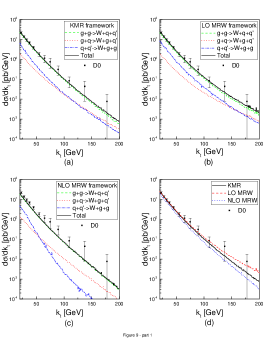
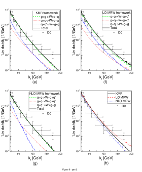
Figure 9: The production rate of the $W^{\pm}$ boson in $E_{CM}=1.8\;TeV$. The labels (a), (b) and (c) compare the contributions of the individual sub-processes in their respective frameworks. The total values of differential cross-section in these frameworks are subjected to a comparison with the data of the $D0$ collaboration D02001 separately, in the label (d). This very same notion is also presented in the labels (e) through (f), where the $1/\sigma\;d\sigma/dk_{t}$ histograms are being compared with each other and with the data from D098 .

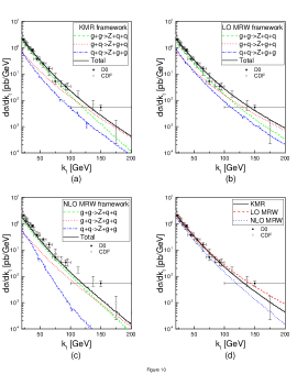
Figure 10: The production rate of the $Z^{0}$ boson in $E_{CM}=1.8\;TeV$. The notions of the diagrams are the same as in the Fig. 9.

Such comparisons can also be made for the larger values of $k_{t}$, see the figures 9 and 10, where the production rates of the electro-weak gauge bosons are plotted against their transverse momentum for $k_{t}<200\;GeV$. The diagrams include the calculations of $d\sigma_{W/Z}/dk_{t}$ and $1/\sigma_{W}\;d\sigma_{W}/dk_{t}$ and the comparisons are made with the help of the data from the $D0$ collaboration, references D098 ; D02001 . Of course, since the data points have small values and large errors, and because of the closeness of the results in different frameworks, one cannot stress over the superiority of any of the approaches. Yet, our previous conclusion about the validity of the $KMR$ $UPDF$ and the short-comings of the $NLO\;MRW$ $UPDF$ holds. Another interesting observation is that in the large $k_{t}$, where because of the smallness of the results the higher order corrections become important, the calculations in the $KMR$ approach start to separate from the $LO\;MRW$ and behave similar to the $NLO\;MRW$. The reason is that the inclusion of the $non-diagonal$ splitting functions into the domain of the $AOC$ introduces some corrections from the $NLO$ region. Additionally, one notices that the contribution coming from the $q+q^{\prime}\to W^{\pm}+g+g$ in the $NLO$ evaluations considerably deviates from the similar behavior of its respective counterparts. This of course roots in the evolution of the $NLO$ quark densities in this framework, see the reference WATT

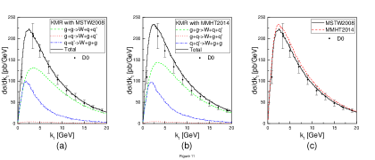
Figure 11: Comparison of the differential cross-section of the $W^{\pm}$ production, using the $UPDF$ of $KMR$, prepared with the $PDF$ of $MSTW2008$ (label (a)) and $MMHT2014$ (label (b)). label (c) shows their difference relative to the experimental data of the $D0$ collaboration, reference D02001 .

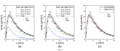
Figure 12: Comparison of the differential cross-section of the $Z^{0}$ production, using the $UPDF$ of $KMR$, prepared with the $PDF$ of $MSTW2008$ (label (a)) and $MMHT2014$ (label (b)). label (c) shows their difference relative to the experimental data of the $D0$ and $CDF$ collaborations, references D098 ; CDF2000 .

Recently, Martin et al have updated their $PDF$ libraries, the reference MMHT . The figures 11 and 12 demonstrate the differences between the cross-section of the production of the $W/Z$ vector bosons in the $KMR$ framework, using the (older) $MSTW2008$ and the (newer) $MMHT2014$ $PDF$. One notices that, using either of these $PDF$ as input for our $UPDF$ produces a negligible difference.

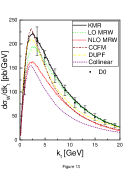
Figure 13: The differential cross-section of the production of the $W^{\pm}$, calculated in different frameworks, against the transverse momentum of the produced gauge boson at $E_{CM}=1.8\;TeV$. The notions of the histograms are as follows: the continues black histogram represents the calculation in using the $KMR$ $UPDF$, the dotted green histogram is prepared in $LO$ $MRW$ framework and the short-dotted red in the $NLO$ $MRW$. To perform these calculations, we have utilized the $PDF$ of $MSTW2008$. the brown dot-dot-dashed histogram in produced using the $CCFM$ $TMD\;PDF$ (reference LIP1 ). The yellow dotted-dashed histogram is calculated, utilizing the doubly unintegrated parton distributions (DUPDF) in the framework of $(k_{t}-z)$-factorization, reference WattWZ . The purple short-dashed histogram is calculated in the collinear framework.

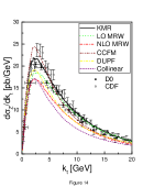
Figure 14: The differential cross-section of the production of the $Z^{0}$, calculated in different frameworks, against the transverse momentum of the produced gauge boson at $E_{CM}=1.8\;TeV$. The notions of the histograms are the same as in Fig.13.

The figures 13 and 14 present an interesting comparison between the experimental data and the results of the different approximations in the calculation of the production of the electro-weak gauge vector bosons. In addition to our calculations in the $KMR$ and the $MRW$ $UPDF$ in the $LO$ and the $NLO$ approximations, the results coming from the $CCFM$ $TMD$ $PDF$ (reference LIP1 ), the $doublly$ $unintegrated$ parton distributions ($DUPDF$, see the reference WattWZ ) and from the $collinear$ frameworks are included in these diagrams. The $CCFM$ results are calculated as the sum of $g+g\to W/Z+q+\bar{q}^{\prime}$, $g+q\to W/Z+q^{\prime}$ and $q+q\to W/Z$ sub-processes. The $DUPDF$ results are in the $(k_{t}-z)$-factorization framework, utilizing a $q+q\to W/Z$ ”effective” production vertex. Furthermore, to calculate the differential cross-section of the $W/Z$ production in the $collinear$ approximation, one have to ignore the transverse momentum integrations in the equation (25) and replace the $UPDF$ with the unpolarized parton distributions of $MSTW2008$, $MMHT2014$ or $GRV2009$ GRV1 ; GRV2 ; GRV3 :

$$\sigma(P+\bar{P}\rightarrow W^{\pm}/Z^{0}+X)=\sum_{a_{i},b_{i}=q,g}\int dp_{b_{1},t}^{2}\;dp_{b_{2},t}^{2}\;dy_{1}\;dy_{2}\;dy_{W/Z}\;{d\varphi_{b_{1}}\over 2\pi}\;{d\varphi_{b_{2}}\over 2\pi}\times$$

$${|\mathcal{M}(a_{1}+a_{2}\rightarrow W/Z+b_{1}+b_{2})|^{2}\over 256\pi^{3}(x_{1}x_{2}s)^{2}}\;a_{1}(x_{1},\mu^{2})\;a_{2}(x_{2},\mu^{2}).$$ (28)

The reader should notice that the results of our computations in the $NLO$ regime, as expected, have a better behavior towards describing the experimental data, both in the $W^{\pm}$ and $Z^{0}$ cases, since they descend with a shallow steep, compared to the results calculated in other schemes. This is in part, because the $NLO$ evaluations are inherently more accurate. Yet, most of the credit goes to the precision of the utilized $UPDF$. Again, the $KMR$ framework in the $NLO$ calculations offers the best description of the experiment.

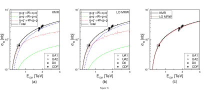
Figure 15: The cross-section of the production of the $W^{\pm}$ bosons as a function of the center-of-mass energy, $E_{CM}$. The experimental data are acquired from the $UA1$, $UA2$, $D0$ and $CDF$ collaborations, references UA1 ; UA2 ; CDF96 ; CDF2000 ; D095 ; D098 ; D02000-1 ; D02000-2 ; D02001 . The calculations are performed using the $KMR$ and the $LO\;MRW$ $UPDF$. We have omitted the $NLO$ $UPDF$ results here, to save computation data.

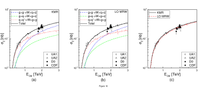
Figure 16: The cross-section of the production of the $Z^{0}$ bosons as a function of the center-of-mass energy, $E_{CM}$. The notation of the diagram is the same as in the figure 15.

Additionally, it is possible to compare our presumed frameworks through the calculation of the total cross-section of the $W^{\pm}$ and $Z^{0}$ production with respect to the center-of-mass energy of the hadronic collision, i.e. the figures 15 and 16. Following our previous pattern, the results of both the $KMR$ and the $LO\;MRW$ frameworks show a good level of compatibility with the experimental data. On the other hand, since the $NLO\;MRW$ framework has failed to describe the data, we have excluded its contributions here, to save some computation time.

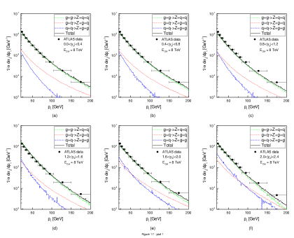
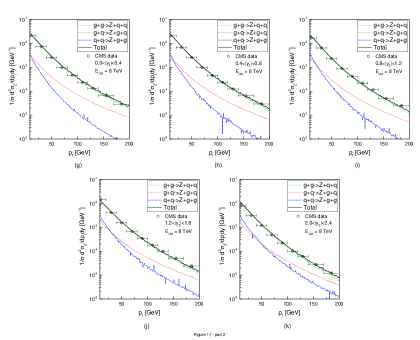
Figure 17: Production of the $Z^{0}$ boson in $E_{CM}=8\;TeV$, using the $KMR$ approach. The individual contributions from the partonic sub-processes are presented and the total values of (single and double) differential cross-sections are subjected to comparison with the data of the $ATLAS$ (black circles) and $CMS$ (white circles) collaborations ATLAS2016 ; CMS2015 . The labels (a) through (f) illustrate the results of our calculations for single differential cross-section of the production of $Z^{0}$, in the given rapidity regions. The results for double differential cross-section are presented in the this figure with labels (g) through (h).

Finally, it has been brought to our attention that the $ATLAS$ and $CMS$ collaborations have recently published some data regarding the production of the $Z^{0}$ gauge vector boson in the $LHC$ for $E_{CM}=8\;TeV$, the references ATLAS2016 ; CMS2015 . In the above calculations, the rapidity of the produced boson has been separated in equally spaced rapidity sectors within $0<|y_{Z}|<2.4$ domain. In figure 17, we have addressed the above observations, using our $NLO$ framework and utilizing the $UPDF$ of $KMR$, since we have already established the superiority of this scheme in describing the experiment. The individual contributions from the partonic sub-processes are presented and the total values of (single and double) differential cross-sections are subjected to comparison with the data of the $ATLAS$ and $CMS$ collaborations. One easily notes that our calculations is in general agreement with the experimental data and with similar calculations in a $NNLO$ $QCD$ framework from the reference NNLOQCD-Z .

Unfortunately, performing these calculations are extremely time-consuming and the existing data points are not plentiful or accurate enough to let us make a decisive statement about the superiority regarding any of our presumed frameworks. Nevertheless, considering these comparisons, it is apparent that the $KMR$ $UPDF$ in the framework of $k_{t}$-factorization, despite their miss-alignments with the theory of the $DGLAP$ evolution equation and the physics of the successive gluon radiations, as an effective theory, proposes the best option to describe the deep inelastic $QCD$ events. However, until further phenomenological analysis, such claim remains as an educated speculation.

In summary, within the present work, we have calculated the rate of productions belonging to the electro-weak gauge vector bosons in the framework of $k_{t}$-factorization, utilizing the $UPDF$ of $KMR$, $LO\;MRW$ and $NLO\;MRW$, by the means of $NLO$ $QCD$ processes. The results have been demonstrated and compared to each other and to the experimental data points from the $D0$ and the $CDF$ collaborations, as well as the calculations in other frameworks. Through our analysis we have suggested that despite the theoretical advantages of the $MRW$ formalism, the $KMR$ approach has a better behavior toward describing the experiment.

Appendix A The matrix elements of the partonic sub-processes

Given that we are interested in the calculation of the matrix element squared for each process, one immediately concludes that the $|\mathcal{M}^{gg}|^{2}=|\mathcal{M}^{qq}|^{2}$. Therefore it is sufficient to calculate the invariant amplitudes for the Feynman diagrams of the figure 2 , the panels (b) and (c), which can be written as follows:

$$\mathcal{M}^{ab}=\sum_{i=1}^{8}\mathcal{M}_{i}^{ab},\;\;\;a,b=q,g,$$ (29)

with

$$\mathcal{M}_{1}^{qg}=g^{2}_{s}\;u(k_{1})\;t^{a}\gamma_{\mu}\epsilon^{\mu}(p_{1})\;{\cancel{(k_{1}-p_{1})}+m\over(k_{1}-p_{1})^{2}-m^{2}}\;G^{\lambda}_{W,Z}\epsilon_{\lambda}(p_{3})\;$$

$${\cancel{(k_{2}+p_{2})}+m\over(k_{2}+p_{2})^{2}-m^{2}}\;t^{b}\gamma_{\nu}\epsilon^{\nu}(k_{2})\;\bar{u}(p_{2}),$$ (30)

$$\mathcal{M}_{2}^{qg}=g^{2}_{s}\;u(k_{1})\;t^{b}\gamma_{\nu}\epsilon^{\nu}(k_{2})\;{\cancel{(k_{1}+k_{2})}+m\over(k_{1}+k_{2})^{2}-m^{2}}\;G^{\lambda}_{W,Z}\epsilon_{\lambda}(p_{3})\;$$

$${\cancel{(k_{2}+k_{2}-p_{3})}+m\over(k_{2}+k_{2}-p_{3})^{2}-m^{2}}\;t^{a}\gamma_{\mu}\epsilon^{\mu}(p_{1})\;\bar{u}(p_{2}),$$ (31)

$$\mathcal{M}_{3}^{qg}=2g^{2}_{s}\;u(k_{1})\;t^{a}\gamma_{\mu}\epsilon^{\mu}(p_{1})\;{\cancel{(k_{1}-p_{1})}+m\over(k_{1}-p_{1})^{2}-m^{2}}\;$$

$$t^{b}\gamma_{\nu}\epsilon^{\nu}(k_{2})\;{\cancel{(p_{2}+p_{3})}+m\over(p_{2}+p_{3})^{2}-m^{2}}\;G^{\lambda}_{W,Z}\epsilon_{\lambda}(p_{3})\;\bar{u}(p_{2}),$$ (32)

$$\mathcal{M}_{4}^{qg}=2g^{2}_{s}\;u(k_{1})\;t^{a}\gamma_{\mu}\epsilon^{\mu}(k_{2})\;{\cancel{(k_{1}+k_{2})}+m\over(k_{1}+k_{2})^{2}-m^{2}}\;$$

$$t^{b}\gamma_{\nu}\epsilon^{\nu}(p_{1})\;{\cancel{(k_{1}+k_{2}-p_{1})}+m\over(k_{1}+k_{2}-p_{1})^{2}-m^{2}}\;G^{\lambda}_{W,Z}\epsilon_{\lambda}(p_{3})\;\bar{u}(p_{2}),$$ (33)

$$\mathcal{M}_{5}^{qg}=g^{2}_{s}\;u(k_{1})\;\gamma^{\rho}C^{\mu\nu\rho}(k_{2},-p_{1},p_{1}-k_{2}){\epsilon_{\mu}\epsilon_{\nu}\over(k_{2}-p_{1})^{2}}f^{abc}t^{c}\;$$

$${\cancel{(p_{2}+p_{3})}+m\over(p_{2}+p_{3})^{2}-m^{2}}\;G^{\lambda}_{W,Z}\epsilon_{\lambda}(p_{3})\;\bar{u}(p_{2}),$$ (34)

$$\mathcal{M}_{6}^{qg}=g^{2}_{s}\;u(k_{1})\;G^{\lambda}_{W,Z}\epsilon_{\lambda}(p_{3})\;{\cancel{(k_{1}-p_{3})}+m\over(k_{1}-p_{3})^{2}-m^{2}}\;$$

$$\gamma^{\rho}C^{\mu\nu\rho}(k_{2},-p_{1},p_{1}-k_{2}){\epsilon_{\mu}\epsilon_{\nu}\over(k_{2}-p_{1})^{2}}f^{abc}t^{c}\;\bar{u}(p_{2}),$$ (35)

and

$$\mathcal{M}_{1}^{gg}=g^{2}_{s}\;\bar{u}(p_{1})\;t^{a}\gamma_{\mu}\epsilon^{\mu}(k_{1})\;{\cancel{(p_{1}-k_{1})}+m\over(p_{1}-k_{1})^{2}-m^{2}}\;G^{\lambda}_{W,Z}\epsilon_{\lambda}(p_{3})\;$$

$${\cancel{(p_{2}+k_{2})}+m\over(p_{2}+k_{2})^{2}-m^{2}}\;t^{b}\gamma_{\nu}\epsilon^{\nu}(k_{2})\;u(p_{2}),$$ (36)

$$\mathcal{M}_{2}^{gg}=g^{2}_{s}\;\bar{u}(p_{1})\;t^{a}\gamma_{\mu}\epsilon^{\mu}(k_{1})\;{\cancel{(k_{2}-p_{1})}+m\over(k_{2}-p_{1})^{2}-m^{2}}\;G^{\lambda}_{W,Z}\epsilon_{\lambda}(p_{3})\;$$

$${\cancel{(k_{1}+p_{2})}+m\over(k_{1}+p_{2})^{2}-m^{2}}\;t^{b}\gamma_{\nu}\epsilon^{\nu}(k_{2})\;u(p_{2}),$$ (37)

$$\mathcal{M}_{3}^{gg}=g^{2}_{s}\;\bar{u}(p_{1}){\cancel{(p_{1}+p_{3})}+m\over(p_{1}+p_{3})^{2}-m^{2}}\;t^{a}\gamma_{\mu}\epsilon^{\mu}(k_{1})\;$$

$${\cancel{(p_{1}+p_{3}-k_{1})}+m\over(p_{1}+p_{3}-k_{1})^{2}-m^{2}}\;G^{\lambda}_{W,Z}\epsilon_{\lambda}(p_{3})\;t^{b}\gamma_{\nu}\epsilon^{\nu}(k_{2})\;u(p_{2}),$$ (38)

$$\mathcal{M}_{4}^{gg}=g^{2}_{s}\;\bar{u}(p_{1})\;G^{\lambda}_{W,Z}\epsilon_{\lambda}(p_{3})\;t^{a}\gamma_{\mu}\epsilon^{\mu}(k_{1})\;{\cancel{(p_{1}-k_{1})}+m\over(p_{1}-k_{1})^{2}-m^{2}}\;$$

$$t^{b}\gamma_{\nu}\epsilon^{\nu}(k_{2})\;{\cancel{(p_{1}-k_{1}-k_{2})}+m\over(p_{1}-k_{1}-k_{2})^{2}-m^{2}}\;u(p_{2}),$$ (39)

$$\mathcal{M}_{5}^{gg}=g^{2}_{s}\;\bar{u}(p_{1})\;G^{\lambda}_{W,Z}\epsilon_{\lambda}(p_{3})\;{\cancel{(p_{1}+p_{3})}+m\over(p_{1}+p_{3})^{2}-m^{2}}\;t^{b}\gamma_{\nu}\epsilon^{\nu}(k_{2})\;$$

$${\cancel{(p_{1}+p_{3}-k_{2})}+m\over(p_{1}+p_{3}-k_{2})^{2}-m^{2}}\;t^{a}\gamma_{\mu}\epsilon^{\mu}(k_{1})\;u(p_{2}),$$ (40)

$$\mathcal{M}_{6}^{gg}=g^{2}_{s}\;\bar{u}(p_{1})\;G^{\lambda}_{W,Z}\epsilon_{\lambda}(p_{3})\;t^{b}\gamma_{\nu}\epsilon^{\nu}(k_{2})\;{\cancel{(p_{1}-k_{2})}+m\over(p_{1}-k_{2})^{2}-m^{2}}\;$$

$$t^{a}\gamma_{\mu}\epsilon^{\mu}(k_{1})\;{\cancel{(p_{1}-k_{1}-k_{2})}+m\over(p_{1}-k_{1}-k_{2})^{2}-m^{2}}\;u(p_{2}),$$ (41)

$$\mathcal{M}_{7}^{gg}=g^{2}_{s}\;\bar{u}(p_{1})\;\gamma^{\rho}C^{\mu\nu\rho}(k_{1},k_{2},-k_{1}-k_{2}){\epsilon_{\mu}\epsilon_{\nu}\over(k_{1}+k_{2})^{2}}f^{abc}t^{c}$$

$${\cancel{(p_{1}-k_{1}-k_{2})}+m\over(p_{1}-k_{1}-k_{2})^{2}-m^{2}}\;G^{\lambda}_{W,Z}\epsilon_{\lambda}(p_{3})\;u(p_{2}),$$ (42)

$$\mathcal{M}_{8}^{gg}=g^{2}_{s}\;\bar{u}(p_{1})\;G^{\lambda}_{W,Z}\epsilon_{\lambda}(p_{3})\;{\cancel{(p_{1}-p_{3})}+m\over(p_{1}-p_{3})^{2}-m^{2}}\;$$

$$\gamma^{\rho}C^{\mu\nu\rho}(k_{1},k_{2},-k_{1}-k_{2}){\epsilon_{\mu}\epsilon_{\nu}\over(k_{1}+k_{2})^{2}}f^{abc}t^{c}\;u(p_{2}),$$ (43)

where $g_{s}$ is the running coupling constant for $QCD$ and $G^{\lambda}_{W,Z}$ represents the vertex of the electro-weak gauge vector bosons with quarks:

$$G^{\lambda}_{W}={e_{em}\over 2\sqrt{2}sin\theta_{w}}\gamma^{\lambda}(1-\gamma^{5})V_{qq^{\prime}}$$

$$G^{\lambda}_{Z}={e_{em}\over sin2\theta_{w}}\gamma^{\lambda}\left[I_{3,q}(1-\gamma^{5})-2e_{q}sin^{2}\theta_{w}\right].$$ (44)

$\theta_{w}$ is the Weinberg angle, $V_{qq^{\prime}}$ is the corresponding $CKM$ matrix element and $I_{3,q}$ is the weak isospin component of the quark $q$. Additionally, the standard $QCD$ three-gluon coupling can be written as follows:

$$C^{\mu\nu\rho}(k_{1},k_{2},k_{3})=g^{\mu\nu}(k_{2}-k_{1})^{\rho}+g^{\nu\rho}(k_{3}-k_{2})^{\mu}+g^{\rho\mu}(k_{1}-k_{3})^{\nu}.$$ (45)

With the above information, one has enough tools to calculate the matrix elements of the equation (25).

References

- (1) V.N. Gribov and L.N. Lipatov, Yad. Fiz., 15 (1972) 781..
- (2) L.N. Lipatov, Sov.J.Nucl.Phys., 20 (1975) 94.
- (3) G. Altarelli and G. Parisi, Nucl.Phys.B, 126 (1977) 298.
- (4) Y.L. Dokshitzer, Sov.Phys.JETP, 46 (1977) 641.
- (5) M.A. Kimber, A.D. Martin and M.G. Ryskin, Phys.Rev.D, 63 (2001) 114027.
- (6) A.D. Martin, M.G. Ryskin, G. Watt, Eur.Phys.J.C, 66 (2010) 163.
- (7) M.A. Kimber, J. Kwiecinski, A.D. Martin, A.M. Stasto, Phys.Rev.D 62, (2000) 094006.
- (8) M.A. Kimber, Unintegrated Parton Distributions, Ph.D. Thesis, University of Durham, U.K. (2001).
- (9) G. Watta, A.D. Martina and M.G. Ryskina, Phys.Rev.D 70 (2004) 014012.
- (10) M. Ciafaloni, Nucl.Phys.B, 296 (1988) 49.
- (11) S. Catani, F. Fiorani, and G. Marchesini, Phys.Lett.B, 234 (1990) 339.
- (12) S. Catani, F. Fiorani, and G. Marchesini, Nucl.Phys.B, 336 (1990) 18.
- (13) M. G. Marchesini, Proceedings of the Workshop QCD at 200 TeV Erice, Italy, edited by L. Cifarelli and Yu.L. Dokshitzer, Plenum, New York (1992) 183.
- (14) G. Marchesini, Nucl.Phys.B, 445 (1995) 49.
- (15) J. Kwiecinski, A.D. Martin, P.J. Sutton,Phys.Rev.D52:1445-1458 (1995).
- (16) V.S. Fadin, E.A. Kuraev and L.N. Lipatov, Phys.Lett.B, 60 (1975) 50.
- (17) L.N. Lipatov, Sov.J.Nucl.Phys., 23 (1976) 642.
- (18) E.A. Kuraev, L.N. Lipatov and V.S. Fadin, Sov.Phys.JETP, 44 (1976) 45.
- (19) E.A. Kuraev, L.N. Lipatov and V.S. Fadin, Sov.Phys.JETP, 45 (1977) 199.
- (20) Ya.Ya. Balitsky and L.N. Lipatov, Sov.J.Nucl.Phys., 28 (1978) 822.
- (21) M. Modarres, H. Hosseinkhani, Nucl.Phys.A, 815 (2009) 40.
- (22) M. Modarres, H. Hosseinkhani, Few-Body Syst., 47 (2010) 237.
- (23) H. Hosseinkhani, M. Modarres, Phys.Lett.B, 694 (2011) 355.
- (24) H. Hosseinkhani, M. Modarres, Phys.Lett.B, 708 (2012) 75.
- (25) M. Modarres, H. Hosseinkhani, N. Olanj, Nucl.Phys.A, 902 (2013) 21.
- (26) M. Modarres, H. Hosseinkhani and N. Olanj, Phys.Rev.D, 89 (2014) 034015.
- (27) M. Modarres, H. Hosseinkhani, N. Olanj and M.R. Masouminia, Eur.Phys.J.C, 75 (2015) 556.
- (28) M. Modarres, M.R. Masouminia, H. Hosseinkhani, and N. Olanj, Nucl.Phys.A, 945 (2016) 168185.
- (29) C. Albajar et al. (UA1 Collaboration), Phys.Lett.B, 253 (1991) 503.
- (30) J. Alitti et al. (UA2 Collaboration), Z.Phys., 47 (1990) 11.
- (31) F. Abe et al. (CDF Collaboration), Phys.Rev.Lett., 76 (1996) 3070.
- (32) B. Affolder et al. (CDF Collaboration), Phys.Rev.Lett., 84 (2000) 845 .
- (33) S. Abachi et al. (D0 Collaboration), Phys.Rev.Lett., 75 (1995) 1456.
- (34) B. Abbott et al. (D0 Collaboration), Phys.Rev.Lett., 80 (1998) 5498.
- (35) B. Abbott et al. (D0 Collaboration), Phys.Rev.D, 61 (2000) 072001.
- (36) B. Abbott et al. (D0 Collaboration), Phys.Rev.D, 61 (2000) 032004.
- (37) B. Abbott et al. (D0 Collaboration), Phys.Lett.B, 513 (2001) 292.
- (38) S. P. Baranov, A.V. Lipatov, and N. P. Zotov, Phys.Rev.D, 78 (2008) 014025.
- (39) M. Deak, Transversal momentum of the electroweak gauge boson and forward jets in high energy factorisation at the , Ph.D. Thesis, University of Hamburg, Germany, 2009.
- (40) A.D. Martin, W.J. Stirling, R.S. Thorne, G. Watt, Eur.Phys.J.C, 63 (2009) 189.
- (41) A.D. Martin, W.J. Stirling, R.S. Thorne, G. Watt, Eur.Phys.J.C, 64 (2009) 653 .
- (42) A.D. Martin, W.J. Stirling, R.S. Thorne, G. Watt, Eur.Phys.J.C, 70 (2010) 51.
- (43) L. A. Harland-Lang, A. D. Martin, P. Motylinski, R.S. Thorne, Eur.Phys.J.C, 75 (2015) 204.
- (44) J. Kwiecinski, A.D. Martin and A.M. Stasto, Phys.Rev.D, 56 (1997) 3991.
- (45) K. Golec-Biernat and A.M. Stasto, Phys.Rev.D, 80 (2009) 014006.
- (46) G. Watt, Parton Distributions, Ph.D. Thesis, University of Durham, U.K. (2004).
- (47) M.A. Kimber, A.D. Martin and M.G. Ryskin, Eur. Phys.J.C, 12 (2000) 655.
- (48) W. Furmanski, R. Petronzio, Phys.Lett.B, 97 (1980) 437.
- (49) S.P. Baranov, A.V. Lipatov and N.P. Zotov, Phys.Rev.D, 81 (2010) 094034.
- (50) A.V. Lipatov and N.P. Zotov, Phys.Rev.D, 81 (2010) 094027; Phys.Rev.D, 72 (2005) 054002.
- (51) J.A.M. Vermaseren, Symbolic Manipulation with FORM, published by Computer Algebra, Nederland, Kruislaan 413, 1098, SJ Amsterdaam, 1991; ISBN 90-74116-01-9.
- (52) M. Cacciari, G. P. Salam and G. Soyez, JHEP 0804 (2008) 063.
- (53) W.-M. Yao et al. (Particle Data Group), J. Phys. G 33, 1 (2006).
- (54) P. Jimenez-Delgado, E. Reya, Phys.Rev.D, 79 (2009) 074023.
- (55) M. Glück, E. Reya, Mod. Phys.Lett.A, 22 (2007) 351.
- (56) P. Jimenez-Delgado, E. Reya, Phys.Rev.D, 80 (2009) 114011.
- (57) ATLAS Collaboration (Georges Aad (Marseille, CPPM) et al.), Eur. Phys. J. C 76(5) (2016) 1-61.
- (58) CMS Collaboration (Vardan Khachatryan (Yerevan Phys. Inst.) et al.), hys. Lett. B 749 (2015) 187.
- (59) A. Gehrmann-De Ridder, T. Gehrmann, E.W.N. Glover, A. Huss, T.A. Morgan, (2016) [arXiv:1605.04295 [hep-ph]].