Torsional oscillations and observed rotational period variations in early-type stars

Abstract

Some chemically peculiar stars in the upper main sequence show rotational period variations of unknown origin. We propose these variations are a consequence of the propagation of internal waves in magnetic rotating stars that lead to the torsional oscillations of the star. We simulate the magnetohydrodynamic waves and calculate resonant frequencies for two stars that show rotational variations: CU Vir and HD 37776. We provide updated analyses of rotational period variations in these stars and compare our results with numerical models. For CU Vir, the length of the observed rotational-period cycle, $\mathit{\Pi}=67.6(5)$ yr, can be well reproduced by the models, which predict a cycle length of 51 yr. However, for HD 37776, the observed lower limit of the cycle length, $\mathit{\Pi}\geq 100$ yr, is significantly longer than the numerical models predict. We conclude that torsional oscillations provide a reasonable explanation at least for the observed period variations in CU Vir.

1 Introduction

Chemically peculiar (CP) stars in the upper main sequence show light variability attributed to rotational modulation of magnetic spots of differing surface abundances. Radiative flux redistribution in the spots results from various bound-free (ionization, Peterson 1970; Lanz et al. 1996) and bound-bound atomic (line, Wolff & Wolff 1971; Trasco 1972; Molnar 1973) transitions. Surface abundance maps derived from Doppler imaging (e.g., Lüftinger et al. 2003; Silvester et al. 2014) can be used to predict the light variability in CP stars (e.g., Krtička et al. 2015; Prvák et al. 2015).

The brightness variability in CP stars allows measurement of their rotational periods. The strict periodicity observed in their light curves allows precise determination of their periods with typical relative uncertainties of the order $10^{-6}$ – $10^{-5}$ (e.g., Adelman 2008). This facilitates the search for very minute changes in the rotational periods. For single CP stars, the usual mechanisms of period change are related to stellar evolution. Unfortunately, evolutionary changes in stellar rotation (Ekström et al. 2012) are not detectable in main-sequence stars (Mikulášek et al. 2014). As a result, most CP stars have very constant rotational periods.

However, there are exceptions. The hottest CP stars with surface magnetic fields and winds may show rotational braking as a result of angular momentum loss via the magnetized stellar wind (ud-Doula et al. 2009). This effect was discovered in the helium-rich star $\sigma$ Ori E by Townsend et al. (2010). Period variations in HD 37776 discovered by Mikulášek et al. (2008a) were also attributed to angular momentum loss. However, subsequent analysis of HD 37776 by Mikulášek et al. (2011a) revealed a significant cubic term in the star’s ephemeris, inconsistent with simple rotational braking. In the CP star CU Vir, intervals of rotational braking were found to alternate with intervals of rotational acceleration by Mikulášek et al. (2011a).

These new findings in stars HD 37776 and CU Vir need to be explained. Here we study the torsional oscillations that result from the interaction of rotation and magnetic field (see Stȩpień 1998, for a similar idea). Although originally introduced for other purposes (cf., Mestel 2012, pages 161–163, see also Mestel & Weiss 1987), we show that the torsional oscillations are able to explain the period variation in CU Vir.

2 Torsional oscillations

We assume that the star is in equilibrium given by the solution of the ideal magnetohydrostatic equation (e.g., Maeder 2009, page 314)

$$0=-\nabla p+\frac{1}{4\pi}(\nabla\times\boldsymbol{B})\times\boldsymbol{B}+\rho\boldsymbol{g}_{\text{eff}}.$$ (1)

The equation is written in a reference frame connected with the star rotating rigidly with angular frequency $\Omega$. Therefore, $\boldsymbol{g}_{\text{eff}}$ stands for effective gravity that results from the gravitational and centrifugal accelerations, and $\boldsymbol{B}$ is the magnetic field.

We will study the incompressible waves in such a star. The velocity and magnetic field perturbation $\delta\boldsymbol{{v}}$ and $\delta\boldsymbol{B}$ shall fulfill the linearized magnetohydrodynamic equations in the form of (c.f., Asai et al. 2016)

$$\nabla\cdot\delta\boldsymbol{{v}} =0,$$ (2)

$$\rho\frac{\partial\delta\boldsymbol{{v}}}{\partial t} =\frac{1}{4\pi}(\nabla\times\delta\boldsymbol{B})\times\boldsymbol{B}+\frac{1}{4\pi}(\nabla\times\boldsymbol{B})\times\delta\boldsymbol{B},$$ (3)

$$\frac{\partial\delta\boldsymbol{B}}{\partial t} =\nabla\times(\delta\boldsymbol{{v}}\times\boldsymbol{B}).$$ (4)

Taking partial derivative of Eq. (3) with respect to time and using Eq. (4) we derive the wave equation

$$\rho\frac{\partial^{2}\delta\boldsymbol{{v}}}{\partial t^{2}}=\frac{1}{4\pi}\{\nabla\times[\nabla\times(\delta\boldsymbol{{v}}\times\boldsymbol{B})]\}\times\boldsymbol{B}+\frac{1}{4\pi}(\nabla\times\boldsymbol{B})\times[\nabla\times(\delta\boldsymbol{{v}}\times\boldsymbol{B})].$$ (5)

As an application of Eq. (5), one can assume an axisymmetric system following Mestel (2012, pages 161–163, see also ) with $\delta\boldsymbol{{v}}\equiv({v}_{R},{v}_{\varphi},{v}_{z})=(0,R\delta\Omega,0)$ and $\boldsymbol{B}\equiv(B_{R},B_{\varphi},B_{z})=(B_{R},0,B_{z})$ in cylindrical coordinates $R$, $\varphi$, and $z$. With constraint $\nabla\cdot\boldsymbol{B}=0$ this leads to the wave equation in the form of (Mestel & Weiss 1987)

$$\rho\,R^{2}\frac{\partial^{2}\delta\mathit{\Omega}}{\partial t^{2}}=\frac{1}{4\pi}\,\boldsymbol{B}\cdot\nabla\left[R^{2}\left(\boldsymbol{B}\cdot\nabla\right)\delta\mathit{\Omega}\right].$$ (6)

We note that the second term on the right-hand side of Eq. (5) is zero because it is given by the vector product of two parallel vectors.

Simple magnetic field configurations are unstable inside the stars (e.g., Braithwaite 2007) and stable internal field is composed of poloidal and toroidal field (Braithwaite & Nordlund 2006). However, there is no analytical description of such complex fields. Consequently, to proceed in the analysis of torsional oscillations in magnetic stars, we selected simple magnetic field configurations, which may not fully describe the internal field.

The general wave equation describing the torsional oscillations Eq. (5) is very complicated, because it involves double curl operator and double vector product. The resulting solution describes 3D oscillations of a star. Therefore, the solution of this equation is cumbersome even for numerical models. However, only the azimuthal component of Eq. (5) is relevant to study the rotational period variations in magnetic stars. Consequently, the easiest way how to proceed is to find such magnetic field configuration, for which only the azimuthal component of the right hand side of Eq. (5) is nonzero. Due to the first term on the right hand side of Eq. (5) including the vector product this can be achieved for magnetic fields with $B_{\varphi}=0$ (in cylindrical coordinates $R$, $\varphi$, and $z$). The simplest form of wave equation contains the derivatives with respect to only one spatial variable (e.g., $R$), for which the angular velocity perturbations are functions of only one spatial variable and time. This is fulfilled for magnetic fields for which the radial component is a function of $R$ only. The constraint $\nabla\cdot\boldsymbol{B}=0$ then yields the magnetic field in the form of $\boldsymbol{B}\equiv(B_{R},B_{\varphi},B_{z})=(B(R),\,0,\,-{z}/{R}\,{\text{d}\!\left(RB(R)\right)}/{\text{d}R})$.

We assume magnetic field that has the above mentioned form,

$$\boldsymbol{B}\equiv(B_{R},B_{\varphi},B_{z})=\left(B,0,-\frac{zB}{R}\right),$$ (7)

where $B$ is constant. Assuming the angular velocity perturbations in the form of $\delta\boldsymbol{{v}}\equiv({v}_{R},{v}_{\varphi},{v}_{z})=(0,R\delta\Omega,0)$ the only nonzero component of Eq. (5) gives the wave equation in the form of

$$\rho\,R^{2}\frac{\partial^{2}\delta\mathit{\Omega}}{\partial t^{2}}=\frac{B^{2}}{4\pi}\,\frac{\partial}{\partial R}\left(R^{2}\frac{\partial\delta\mathit{\Omega}}{\partial R}\right).$$ (8)

For $R\,{\partial^{2}\delta\mathit{\Omega}}/{\partial R^{2}}\gg{\partial\delta\mathit{\Omega}}/{\partial R}$ the wave speed is equal to the Alfvén speed, $\varv_{\text{A}}=B/\!\sqrt{4\pi\rho}$. The field lines of the adopted magnetic field Eq. (7) lie in the equatorial plane for $z=0$ and the more they lie above (or below) the equatorial plane the more they diverge from the horizontal plane $z=\text{const.}$ The magnetic field has therefore a goblet-like structure. The Alfvén waves propagate along the field lines and cause the torsional oscillations that are perpendicular to the magnetic field. The field lines of Eq. (7) are also normal to the stellar surface at the equatorial plane, therefore the amplitude of torsional oscillation is large in this region. The adopted magnetic field has an internal stellar field that is similar in strength to the surface field, which is not the case of dipole field model.

The wave equation (8) preserves its form for the scale transformations $\boldsymbol{B}^{\prime}=\gamma\boldsymbol{B}$ and $t^{\prime}=\gamma^{-1}t$, where $\gamma$ is a constant. This means that the solution of the wave equation for a given star is the same as the solution for a magnetic field scaled by factor $\gamma$ at a time scaled by $\gamma^{-1}t$.

A similar problem for more complex fields also leads to the wave equation and resonant modes described in the following text. Wave equations similar to Eq. (8) can be obtained also for homogeneous magnetic field $\boldsymbol{B}=\text{const.}$ or for magnetic field of Roberts (1981, see ), that in spherical coordinates reads $\boldsymbol{B}\equiv(B_{r},B_{\vartheta},B_{\varphi})=(B/2\cos\theta(5-3r^{2}/R_{*}^{2}),B/2\sin\theta(6r^{2}/R_{*}^{2}-5),0)$ with $B$ being constant.

3 Numerical simulation of torsional oscillations

For numerical simulations we have rewritten Eq. (8) in a flux-conservative form

$$\frac{\partial\boldsymbol{u}}{\partial t}=\mathsf{F}\,\frac{\partial\boldsymbol{u}}{\partial R},$$ (9)

where $\boldsymbol{u}\equiv(u_{1},u_{2})^{\text{T}}=({\partial\delta\mathit{\Omega}}/{\partial t},\,R^{2}B\,{\partial\delta\mathit{\Omega}}/{\partial R})^{\text{T}}$ and $\mathsf{F}$ is a matrix

$$\mathsf{F}=\left(\begin{array}[]{cc}0&\displaystyle\frac{B}{4\pi\rho R^{2}}\\ R^{2}B&0\\ \end{array}\right).$$ (10)

The density distribution for the solution of Eq. (9) was taken from the MESA stellar evolutionary models (Paxton et al. 2011, 2013). The boundary conditions were selected in a same fashion as boundary conditions for stellar pulsations (Maeder 2009). We anticipate that $\delta\mathit{\Omega}$ is constant close to the stellar surface, therefore we assume a solid wall boundary condition for $\partial\delta\mathit{\Omega}/{\partial R}$ (or $u_{2}$), whereas we assume reflecting boundary condition for the inner boundary condition. Because the variables $u_{1}$ and $u_{2}$ are connected with a derivative, we selected the boundary conditions for $u_{1}$ in the opposite manner, i.e., reflecting boundary condition at the outer boundary and solid wall boundary condition at the inner boundary. We introduce the external forcing at the inner boundary, which seems to be more physically meaningful.

The model equations are solved for $z=0$. The wave equation is independent of $z$, however the boundary conditions and consequently also the derived resonance frequencies depend on $z$. We discuss the implications of this assumption in Sect. 6.

We solved Eq. (9) numerically using the leapfrog method (Press et al. 2005). We used $N$ equidistantly spaced grid points $R_{1},\,R_{2},\dots,R_{N}$ within the stellar radius. We assumed no initial perturbation, $\boldsymbol{u}(R,t=0)=0$. The inner boundary conditions (at $R=R_{1}$) with external forcing were represented as

$$u_{1}(R_{1},t) =-u_{1}(R_{2},t)+A_{1}\sin(\omega t),$$ (11)

$$u_{2}(R_{1},t) =u_{2}(R_{2},t)-A_{2}\sin(\omega t),$$ (12)

where $\omega$ is the frequency of external forcing and $A_{1}$ and $A_{2}$ its amplitudes. The subscripts of $u$ denote its components, and the subscript of the radius denotes individual grid points. We selected $R_{1}$ corresponding to the inner convection zone as derived from the MESA models. The outer boundary conditions (at $R=R_{N}$) are represented as

$$u_{1}(R_{N},t) =u_{1}(R_{N-1},t),$$ (13)

$$u_{2}(R_{N},t) =-u_{2}(R_{N-1},t).$$ (14)

To avoid instabilities, the Courant-Friedrichs-Lewy condition was used to limit the length of the time step. The selected time step was a fraction of the minimum travel time of Alfvén waves across one grid zone.

We used $N=1000$ in our calculations. Because the Alfvén waves are very fast close to the stellar surface, the time step required by the Courant-Friedrichs-Lewy condition is very short, which results in a prohibitively short time step for the calculations. To make the calculations more tractable, we omit the surface layers from our calculations. Since this typically corresponds to a very small fraction of the stellar radius, this modification does not strongly affect the final results. Because the wave equation (8) is linear, the absolute scale of the external forcing amplitudes $A_{1}$ and $A_{2}$ is unimportant for the subsequent numerical analysis.

4 Application of numerical simulations to individual stars

4.1 CU Vir

An abrupt period increase in CU Vir (HD 124224) was reported by Pyper et al. (1998, 2013). On the other hand, Mikulášek et al. (2011a) found evidence in the available photometric and spectrophotometric measurements for gradual long-term period variations (see also Stȩpień 1998) and even detected intervals where the period was decreasing. We assumed the latter model of the period variations. For our analysis we selected the MESA solar-metallicity evolutionary model with an initial mass of $3\,M_{\odot}$ at the age of $9\times 10^{7}\,\text{yr}$, which corresponds to CU Vir parameters derived by Kochukhov & Bagnulo (2006). We adopted $B_{\text{p}}=1\,\text{kG}$, which is representative of CU Vir’s surface (Kochukhov et al. 2014). The radial boundaries of the computational zone are at $R_{1}=0.159\,R_{*}$ and $R_{N}=0.997\,R_{*}$, where $R_{*}$ is the stellar radius as calculated by MESA models.

Figure 1: The waves connected with torsional oscillations in the model stellar interior of CU Vir for $\omega=3.76\times 10^{-8}\,\text{s}^{-1}$, which corresponds to resonance. Upper panel: The variable $u_{1}$ at different stages of the wave evolution. The curves are denoted by the elapsed time in units of the period of external forcing $\mathit{\Pi}=2\pi/\omega\approx 5.3\,\text{yr}$. Middle panel: The behavior of $u_{1}$ at the outer boundary of the model. Lower panel: The evolution of $\delta\Omega$ derived from the numerical integration of $u_{1}$.

In Fig. 1 we plot the solution to the wave equation (8) for $\omega=3.76\times 10^{-8}\,\text{s}^{-1}$ (corresponding to a resonate overtone, see below), $A_{1}=1\,\text{s}^{-2}$, and $A_{2}=1\,\text{cm}^{1/2}\,\text{g}^{1/2}\,\text{s}^{-2}$. The upper panel shows wave solutions that grow in amplitude. The wave form remains roughly constant with four knots for a specific value of $\omega$. The lower panel shows the outer boundary oscillating with a frequency $\omega$ and a growing amplitude.

The observed frequencies are those with the largest growth rates and are eigenfrequencies of the corresponding oscillator. Therefore, we scanned all frequencies in the range of $\omega=10^{-9}\,\text{s}^{-1}$ – $10^{-7}\,\text{s}^{-1}$ to find the maximum growth rate of the oscillations. The selected frequencies roughly correspond to those detectable from observations with period $\mathit{\Pi}=2$ – $200\,\text{years}$. We allowed the system to evolve for $T=600\,$years. The magnitude of the oscillations is estimated from the variable $\langle u_{1}^{2}\rangle$, defined as a mean value of the square of $u_{1}$ averaged over the period $\mathit{\Pi}=2\pi/\omega$,

$$\langle u_{1}^{2}\rangle=\frac{1}{\mathit{\Pi}}\int_{T-\mathit{\Pi}}^{T}u_{1}^{2}(R_{N},t)\,\text{d}t.$$ (15)

Figure 2: The dependence of the scale mean-squared wave amplitude at the stellar surface (see Eq. (15)) on the frequency after $T=600\,$years of wave evolution for CU Vir. The upper axis is labeled with corresponding oscillation periods.

In Fig. 2 we plot the results of the simulations. The amplitude of $\langle u_{1}^{2}\rangle$ has several sharp peaks at the basic frequency of the oscillator and its overtones. There is a maximum amplitude at the period of about 51 years with overtones at higher frequencies. The first overtones correspond to periods 15, 9, 7, and 5 years. The basic period of 51 yr is roughly four times as long as the Alfvén wave travel time between the boundaries of the computational zone, which is 15 years. Therefore, in the basic mode the computational zone accommodates one fourth of the wave with a node at the inner boundary and an antinode at the outer boundary. We note that it might be better to scale $\langle u_{1}^{2}\rangle$ by $\omega^{-1}$ in Fig. 2 to account for an $\omega$ dependence of power on external forcing Eq. (13), but this has little impact on the final results, because the derived peaks are relatively sharp.

4.2 HD 37776

Rotational period variations in HD 37776 (V901 Ori) were detected by Mikulášek et al. (2008a). A subsequent study by Mikulášek et al. (2011a) provided additional support for complex period variations in this star. For our analysis, we selected the MESA solar-metallicity evolutionary model with an initial mass of $8\,M_{\odot}$ and an age of $3\times 10^{6}\,\text{yr}$. This corresponds to HD 37776 parameters (Landstreet et al. 2007; Mikulášek et al. 2008a). The star has a very complex surface magnetic field (Kochukhov et al. 2011); consequently we selected $B_{\text{p}}=10\,\text{kG}$, which roughly corresponds to the observed values. We selected $R_{1}=0.203\,R_{*}$ and $R_{N}=0.983\,R_{*}$ for the outer model radius, where $R_{*}$ is the stellar radius as calculated by MESA models.

Figure 3: Model of waves connected with torsional oscillations in a stellar interior corresponding to HD 37776 for $\omega=1.1\times 10^{-7}\,\text{s}^{-1}$, which is slightly out of the resonance. Upper panel: The variable $u_{1}$ at different stages of the wave evolution. The curves are denoted by the elapsed time in units of the period of external forcing $\mathit{\Pi}=2\pi/\omega\approx 1.8\,\text{yr}$. Middle panel: The behavior of $u_{1}$ at the outer boundary of the model. Lower panel: The evolution of $\delta\Omega$ derived from the numerical integration of $u_{1}$.

In Fig. 3 we plot the solution of wave equation (8) for $\omega=1.1\times 10^{-7}\,\text{s}^{-1}$, $A_{1}=1\,\text{s}^{-2}$, and $A_{2}=1\,\text{cm}^{1/2}\,\text{g}^{1/2}\,\text{s}^{-2}$. The selected frequency is slightly out of the resonance. The upper panel shows a wave solution with variable amplitude. The wave form remains roughly constant with one knot (for a given value of $\omega$). The lower panel of Fig. 3 shows that the outer boundary oscillates with frequency $\omega$ and an amplitude affected by beating between the period of external forcing and the eigenfrequency of the oscillator.

We scanned all frequencies in the range $\omega=10^{-9}\,\text{s}^{-1}$ – $10^{-6}\,\text{s}^{-1}$ to find the maximum growth rate of the oscillations. We let the system evolve for $T=600\,$years. The resulting mean value of the outer boundary amplitude averaged over the last period of simulations $\langle u_{1}^{2}\rangle$ (see Eq. (15)) is given in Fig. 4. The first three resonance frequencies correspond to periods of 5, 1.6, and 1 yr. In this case, the basic 5 yr period of torsional oscillations is roughly four times the Alfvén wave travel time between the boundaries of the computational zone, which is 1.6 years. The periods of oscillations are significantly shorter than in the case of CU Vir due to stronger surface magnetic field in HD 37776. This can be seen already from the scaling relations given in Sect. 2 and from the results obtained for CU Vir in Sect. 4.1.

Figure 4: Same as Fig. 2, but for HD 37776.

5 Comparison of numerical results with observations

To date, rotational period variations of chemically peculiar stars were phenomenologically described by simple polynomials and their combinations. Our proposed explanation of the observed period variations requires a new analysis of the data assuming sinusoidal period variations (Mikulášek et al. 2011b).

The variations of the rotational period of CU Vir are derived from the analysis of 18 267 individual photometric, spectroscopic, and radiometric observations obtained from 1949 to 2015 (Mikulášek et al. 2011a, 2014), supplemented by additional new $BV$ observations from the T3 0.4 m Automatic Photoelectric Telescope (APT) at Fairborn Observatory in southern Arizona. The available observations together with updated analysis of the period changes will be described in a separate paper in detail (Mikulášek et al., in preparation). We found that the instantaneous rotational period $P(t)$ varied nearly harmonically according to the simple relation

$$P(t)=P_{0}+A\,\sin\left(2\,\pi\,\frac{t-\mathit{\Theta_{0}}}{\mathit{\Pi}}\right),$$ (16)

where $t$ is a JDhel time, $P_{0}=0\aas@@fstack{d}52069424(4)$ is the mean rotational period, $A=2\aas@@fstack{d}167(8)\times 10^{-5}=1.872(7)$ s is the semiamplitude of period variations, $\mathit{\Theta_{0}}=2\,4466\,530(16)=1986.69(5)$, and $\mathit{\Pi}=24\,680(190)$ d $=67.6(5)$ years, is the length of the period cycle $P(t)$. The semiamplitude of the cyclic (O-C) changes

$$A_{\mathrm{OC}}=\frac{A\,\mathit{\Pi}}{2\,\pi\,\overline{P}}$$ (17)

is $A_{\mathrm{OC}}=0\aas@@fstack{d}1635=0.31\,\overline{P}$. The period changes and the phase shifts in days are presented in Fig. 5. Our observations extend nearly over the entire cycle of period changes.

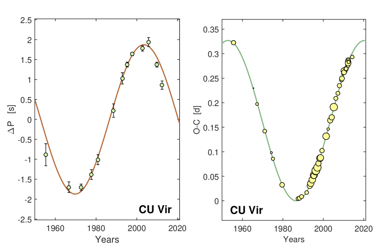
Figure 5: Variations of the rotational period in seconds and phase shifts in days for CU Vir in the time interval 1949 – 2015. The observed values are fitted by simple sine/cosine model with a period of $\mathit{\Pi}=67.6$ years.

The predicted period of torsional oscillations in CU Vir agrees well with time scale of period variations observed in this star. Moreover, the period variations on the scale of ten years (Mikulášek et al. 2011a) can be nicely explained by the higher overtones of the torsional oscillations. Consequently, the torsional oscillations provide a viable explanation of the period variations found in CU Vir.

Our second hot CP star with pronounced period variations is HD 37776 (V901 Ori). Its period analysis is based on 3483 photometric and spectroscopic observations obtained between 1976 and 2014 (Mikulášek et al. 2011a, 2014) supplemented by additional new $BV$ observations from the T3 0.4 m APT. We find that changes of its instantaneous rotational period of $P(t)$ can be well approximated by a parabola or a segment of a harmonic function of period $\mathit{\Pi}$ with a maximum at the time $T_{\mathrm{max}}$:

$$P(t)=P_{\mathrm{max}}+A\,\left[\cos\left(2\,\pi\,\frac{t-T_{\mathrm{max}}}{\mathit{\Pi}}\right)-1\right],$$ (18)

where $P_{\mathrm{max}}$ is the maximum rotational period, and the semiamplitude of the corresponding cyclic variations of (O-C) is given by Eq. (17).

We are not able to determine the true value of the period cycle $\mathit{\Pi}$, only its lower limit: $\mathit{\Pi}\geq 100$ years. Therefore, $P_{\mathrm{max}}\cong 1\aas@@fstack{d}538784$, $A\geq 1\aas@@fstack{d}42\times 10^{-4}=12.2$ s, $A_{\mathrm{OC}}\geq 0\aas@@fstack{d}54=0.35\,\overline{P}$, and $T_{\mathrm{max}}\geq 2006.5$, and HJD$(T_{\mathrm{max}})=2\,453\,910$.

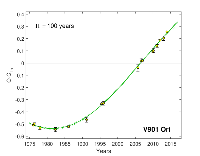
Figure 6: The observed phase shifts in days for V901 Ori fitted with a sine function with the minimal acceptable period $\mathit{\Pi}=100$ years.

For HD 37776 the predicted torsional oscillation period cycle is significantly shorter than the observed period cycle. This might be explained by a difference between the surface and inner magnetic field. The surface field of HD 37776 is very complex (Kochukhov et al. 2011), and it may decay over time as seen in magnetic stars found in open clusters (Landstreet et al. 2007). It is possible that part of the observed decay may be connected with equalization of the surface and inner magnetic field. However, it does not follow from the simulations that the surface field is stronger than the inner field (Braithwaite & Nordlund 2006).

On the other hand, there are still other possibilities that can explain the observed period variations. Besides that excluded by Mikulášek et al. (2008a), the most relevant could be the tidal interaction with an orbiting low-mass body (Mardling 2007). For example, a possible scenario could include a low-mass object on a non-synchronized precessing orbit. We postpone this possibility for a future detailed study.

6 Discussion

The model presented in this paper includes only the basic physics describing the problem. Moreover, we solve the wave equation for $z=0$ only. In reality, the internal magnetic field has a more complex structure, and stable internal magnetic fields are given by the combination of poloidal and toroidal magnetic fields (see Braithwaite & Nordlund 2006 and Braithwaite & Spruit 2015, for a review). Because the wave equation (8) is specified on the field lines a more realistic field topology would lead to a lengthening of the oscillation period on each field line (see also Link & van Eysden 2016). As the basic frequency differs on each field line, the basic frequency of the global mode will be given by a weighted average of individual frequency modes. The resulting phase mixing (e.g., Heyvaerts & Priest 1983) may lead to the damping of oscillations, but since the individual peaks in the periodogram are rather broad (see Fig. 2), we expect that the oscillations may still be observable.

The magnetic field dominates the atmospheres of studied stars. Therefore, their surface may resemble the crust of neutron stars forcing the individual field lines to oscillate with the same frequency. Consequently, the variations of rotational period of CP stars may have the same explanation as quasi-periodic oscillations of neutron stars. In this case the frequencies of rotational period variations may be associated with turning points or edges of the MHD continuum (Levin 2007) or with normal oscillation modes (Lee 2008).

Another problem is connected with existence of two shallow convection zones associated with local opacity enhancements inside massive stars (e.g., Maeder et al. 2008). However, because these zones contain only a very small fraction of the stellar mass, we expect that their existence does not significantly alter our results.

Our model assumes small perturbations of otherwise uniform stellar angular velocity. This does not seem to be in contradiction with vertical differential rotation profiles derived from asteroseismology in BA stars (Briquet et al. 2007; Kurtz et al. 2014). However, angular momentum transport by, e.g., internal gravity waves (Rogers 2015) may lead to damping of torsional oscillations.

It is not clear what mechanism drives the torsional oscillations. The forcing mechanism may be connected either with the core convection zone or with winds blowing from the stellar surface. If some Ap stars originate in binary star mergers (Maitzen et al. 2008; Bogomazov & Tutukov 2009), then subsequent relaxation processes may provide a convenient mechanism that drives the torsional oscillations. This would mean that CU Vir is a merger product. This could possibly provide a consistent explanation of circumstellar matter that is required to power the pulsed radio emission observed in CU Vir (Trigilio et al. 2000; Kellett et al. 2007). An alternative explanation of line-driven wind mass-loss rate of about $10^{-12}\,{M}_{\odot}\,\text{yr}^{-1}$ (Leto et al. 2006) is problematic due to the low effective temperature of the star (Krtička 2014).

The wave equation (8) is linear and so allows oscillations with arbitrary amplitudes. This is unrealistic in nature, and several processes may lead to damping of strong oscillations. One obvious process is reconnection, which may occur in the case of oscillations that are wound up too much. The oscillations may also be damped due to vertical shear.

Another important question is connected with the fact that period variations are detected in only a handful of magnetic stars, while the light curves of most of them are adequately described with constant periods (e.g., Adelman 2008; Mikulášek et al. 2008b; Wraight et al. 2012; Bernhard et al. 2015). While a lack of suitable long observing series may provide an obvious answer for many stars, more subtle reasons may be missing. However, since a similar question is not clearly resolved in many notorious classical pulsating stars, i.e., the question why there are stars that do not pulsate in the instability strip (e.g., Fontaine et al. 2006; Balona et al. 2011; Saio et al. 2013), we postpone this question for a future study.

7 Conclusions

We simulated stellar torsional oscillations that result from the interaction of the internal magnetic field and differential rotation. The simulations were calculated for the chemically peculiar stars CU Vir and HD 37776, which both have rotational period variations. We derived the internal structure of individual modes and calculated the wave resonance frequencies, for which the amplitudes of surface angular frequency variations are the largest. For each star we found a basic frequency and several high-order overtones.

We provide a new analysis of period variations in the stars CU Vir and HD 37776 assuming periodic rotational period variations. For CU Vir, the length of the rotational period cycle $\mathit{\Pi}=67.6(5)$ yr can be well reproduced by numerical models, which predict a cycle length of 51 yr. The numerical model also predicts the variations on the scale of about 10 yr in agreement with observations. Consequently, the torsional oscillations provide a reasonable explanation of the observed period variations of CU Vir. On the other hand, for HD 37776 the observed lower limit of the period cycle, $\mathit{\Pi}\geq 100$ yr, is significantly longer than the predicted cycle length of 5 yr. It is immediately clear from the scaling of the wave equation with the magnetic field and from the observed strength of the field that the model cannot reproduce the observations of both stars. There may be other possible explanations for the observed period variations in HD 37776.

References

- Adelman (2008) Adelman, S. J. 2008, PASP, 120, 367
- Asai et al. (2016) Asai H., Lee U., & Yoshida, S., 2016, MNRAS, 455, 2228
- Balona et al. (2011) Balona L. A., Pigulski A., Cat P. D., et al., 2011, MNRAS, 413, 2403
- Bernhard et al. (2015) Bernhard K., Hümmerich S., Paunzen E., 2015, AN, 336, 981
- Bogomazov & Tutukov (2009) Bogomazov A. I., & Tutukov A. V. 2009, Astronomy Reports, 53, 214
- Braithwaite (2007) Braithwaite J., 2007, A&A, 469, 275
- Braithwaite & Nordlund (2006) Braithwaite J., & Nordlund, Å., 2006, A&A, 450, 1077
- Braithwaite & Spruit (2015) Braithwaite J., & Spruit, H. C., 2015, arXiv:1510.03198
- Briquet et al. (2007) Briquet M., Morel T., Thoul A., et al., 2007, MNRAS, 381, 1482
- Ekström et al. (2012) Ekström S., Georgy C., Eggenberger P., et al., 2012, A&A, 537, A146
- Fontaine et al. (2006) Fontaine G., Green E. M., Chayer P., et al. 2006, Baltic Astronomy, 15, 211
- Heyvaerts & Priest (1983) Heyvaerts J., & Priest E. R., 1983, A&A, 117, 220
- Kellett et al. (2007) Kellett B. J., Graffagnino V., Bingham R., Muxlow T. W. B., & Gunn G. A. 2007, arXiv:astro-ph/0701214v1
- Kochukhov & Bagnulo (2006) Kochukhov O., & Bagnulo S. 2006, A&A, 450, 763
- Kochukhov et al. (2011) Kochukhov O., Lundin A., Romanyuk I., & Kudryavtsev D., 2011, ApJ, 726, 24
- Kochukhov et al. (2014) Kochukhov O., Lüftinger T., Neiner C., Alecian E., & MiMeS Collaboration 2014, A&A, 565, A83
- Krtička (2014) Krtička J., 2014, A&A, 564, A70
- Krtička et al. (2015) Krtička J., Mikulášek Z., Lüftinger T., & Jagelka M., 2015, A&A, 576, A82
- Kurtz et al. (2014) Kurtz D. W., Saio H., Takata M., et al., 2014, MNRAS, 444, 102
- Landstreet et al. (2007) Landstreet J. D., Bagnulo S., Andretta V., et al. 2007, A&A, 470, 685
- Lanz et al. (1996) Lanz T., Artru M.-C., Le Dourneuf M., & Hubeny I. 1996, A&A, 309, 218
- Lee (2008) Lee U., 2008, MNRAS, 385, 2069
- Leto et al. (2006) Leto P., Trigilio C., Buemi C. S., Umana G., & Leone F. 2006, A&A, 458, 831
- Levin (2007) Levin Y., 2007, MNRAS, 377, 159
- Link & van Eysden (2016) Link, B., & van Eysden, C. A. 2016, ApJ, 823, L1
- Lüftinger et al. (2003) Lueftinger T., Kuschnig R., Piskunov N. E., & Weiss W. W. 2003, A&A, 406, 1033
- Maeder (2009) Maeder A. 2009, Physics, Formation and Evolution of Rotating Stars (Springer, Berlin)
- Maeder et al. (2008) Maeder A., Georgy C., & Meynet, G., 2008, A&A, 479, L37
- Maitzen et al. (2008) Maitzen H. M., Paunzen E., & Netopil M., 2008, Contributions of the Astronomical Observatory Skalnate Pleso, 38, 385
- Mardling (2007) Mardling R. A., 2007, MNRAS, 382, 1768
- Mestel (2012) Mestel L. 2012, Stellar Magnetism (Oxford, Oxford University Press)
- Mestel & Weiss (1987) Mestel L., & Weiss N. O., 1987, MNRAS, 226, 123
- Mikulášek et al. (2008a) Mikulášek Z., Krtička J., Henry G. W. et al. 2008a, A&A, 485, 585
- Mikulášek et al. (2008b) Mikulášek Z., Gráf T., Krtička J., Zverko J., Žižňovský J., 2008b, CoSka, 38, 363
- Mikulášek et al. (2011a) Mikulášek Z., Krtička, J., Henry G. W. et al. 2011a, A&A, 534, L5
- Mikulášek et al. (2011b) Mikulášek Z., Krtička J., Janík J., et al., 2011b, Magnetic Stars, 52
- Mikulášek et al. (2014) Mikulášek Z., Krtička J., Janík J., et al., 2014, Putting A Stars into Context: Evolution, Environment, and Related Stars, 270
- Molnar (1973) Molnar M. R. 1973, ApJ, 179, 527
- Paxton et al. (2011) Paxton B., Bildsten, L., Dotter A., et al., 2011, ApJS, 192, 3
- Paxton et al. (2013) Paxton B., Cantiello, M., Arras P., et al., 2013, ApJS, 208, 4
- Peterson (1970) Peterson D. M. 1970, ApJ, 161, 685
- Press et al. (2005) Press W. H, Teukolsky S. A., Vetterling, W. T., & Flannery B. P. 2005, Numerical recipies in C++ (Cambridge, Cambridge University Press)
- Prvák et al. (2015) Prvák M., Liška J., Krtička J., Mikulášek Z., Lüftinger, T., 2015, A&A, 584, A17
- Pyper et al. (1998) Pyper D. M., Ryabchikova T., Malanushenko V., et al., 1998, A&A, 339, 822
- Pyper et al. (2013) Pyper D. M., Stevens, I. R., & Adelman S. J., 2013, MNRAS, 431, 2106
- Roberts (1981) Roberts P. H., 1981, AN, 302, 65
- Rogers (2015) Rogers T. M., 2015, ApJ, 815, L30
- Saio et al. (2013) Saio H., Georgy C., & Meynet G., 2013, MNRAS, 433, 1246
- Silvester et al. (2014) Silvester J., Kochukhov O., & Wade G. A., 2014, MNRAS, 444, 1442
- Stȩpień (1998) Stȩpień K., 1998, A&A, 337, 754
- Townsend et al. (2010) Townsend R. H. D., Oksala M. E., Cohen D. H., Owocki S. P., & ud-Doula A. 2010, ApJ, 714, 318
- Trasco (1972) Trasco J. D. 1972, ApJ, 171, 569
- Trigilio et al. (2000) Trigilio C., Leto P., Leone F., Umana G., & Buemi C. S. 2000, A&A, 362, 28
- ud-Doula et al. (2009) ud-Doula A., Owocki S. P., & Townsend R. H. D. 2009, MNRAS, 392, 1022
- Wolff & Wolff (1971) Wolff S. C., & Wolff R. J. 1971, AJ, 76, 422
- Wraight et al. (2012) Wraight K. T., Fossati L., Netopil M., Paunzen E., Rode-Paunzen M., Bewsher D., Norton A. J., White G. J., 2012, MNRAS, 420, 757