Pickands’ constant at first order in an expansion around Brownian motion

Abstract

In the theory of extreme values of Gaussian processes, many results are expressed in terms of the Pickands constant $\mathcal{H}_{\alpha}$. This constant depends on the local self-similarity exponent $\alpha$ of the process, i.e. locally it is a fractional Brownian motion (fBm) of Hurst index $H=\alpha/2$. Despite its importance, only two values of the Pickands constant are known: ${\cal H}_{1}=1$ and ${\cal H}_{2}=1/\sqrt{\pi}$. Here, we extend the recent perturbative approach to fBm to include drift terms. This allows us to investigate the Pickands constant $\mathcal{H}_{\alpha}$ around standard Brownian motion ($\alpha=1$) and to derive the new exact result $\mathcal{H}_{\alpha}=1-(\alpha-1)\gamma_{\rm E}+\mathcal{O}\!\left(\alpha-1\right)^{2}$.

1 Introduction: Maximum of a Gaussian process

The extreme-value statistics of strongly correlated variables is an active research field. However, only few general theorems for the maximum of a set of such variables are known. Notable exceptions are random walks [1, 2], the free energy of a directed polymer on a tree [3], the eigenvalues of a random matrix [4], or the extreme-values of specific Gaussian processes [5, 6, 7, 8].

For generic Gaussian Random Processes, the tail of the distribution for large values of the maximum has been studied notably by Pickands and Piterbarg, and led to the definition of what is now known as the Pickands constant, and which continues to be studied [9, 10, 11, 12].

To appreciate the high degree of universality of the theorems involved, we first state the original theorem of Pickands [13], formulated for stationary processes: Consider a stationary Gaussian process $X_{t}$ with mean $\mathbb{E}(X_{t})=0$, and normalized squared variance ${\mathbb{E}(X_{t}^{2})}=1$. By assumption, the covariance function

$$r(t):=\mathbb{E}\left(X_{t_{0}}X_{t_{0}+t}\right)$$ (1)

is independent of $t_{0}$. Suppose that it satisfies

$$r(t) < 1\qquad\qquad\forall t>0\ ,$$ (2)

$$r(t) \simeq 1-|t|^{\alpha}~{}~{}~{}~{}~{}~{}\mbox{for~{}}t\to 0\ .$$ (3)

Condition (2) excludes that the process is periodic, while condition (3) sets the scales for $X_{t}$ and $t$ and defines the exponent $\alpha$. Under these circumstances, one has [13]

Theorem (Pickands 1969):

$$\mathbb{P}\!\left(\max_{t\in[0,T]}X_{t}>u\right) \simeq \Psi(u)Tu^{2/\alpha}{\cal H}_{\alpha}\quad\mbox{as }\;u\to\infty$$ (4)

$$\mbox{~{}~{}~{}~{}~{}~{}~{}~{} with }~{}\Psi(u) := \frac{1}{2\pi}\int_{u}^{\infty}\exp\!\left(-\frac{x^{2}}{2}\right)\rmd x$$ (5)

$$\mbox{ ~{}~{}~{}~{}~{}~{}~{}~{} and }~{}~{}~{}~{}{\cal H}_{\alpha} := \lim_{T\to\infty}\frac{1}{T}\mathbb{E}\!\left(\exp\!\left(\max\limits_{0<t<T}\chi_{t}\right)\right)\ .$$ (6)

The first term on the r.h.s. of Eq. (4), $\Psi(u)$, is an integrated Gaussian as expected from intuition, or more rigorously from the Borel inequality [14]. The factor $T$ expresses the fact that the tail is dominated by events localized in time, and thus proportional to $T$. The non-trivial statement is that the amplitude can be calculated from a specific process $\chi_{t}$ depending only on $\alpha$, and that the limit (6) exists.

To define $\chi_{t}$, we first recall the definition [15] of a fractional Brownian motion (fBm) with Hurst exponent $H=\alpha/2$, denoted $B_{t}$: It is a Gaussian process starting at the origin, $B_{0}=0$, with mean zero, $\mathbb{E}(B_{t})=0$, and covariance function

$$\mathbb{E}\left(B_{t}B_{s}\right)=|t|^{\alpha}+|s|^{\alpha}-|t-s|^{\alpha}\ .$$ (7)

The process $\chi_{t}$ is then defined as a fBm with drift,

$$\chi_{t}:=B_{t}-\frac{1}{2}\mathbb{E}(B_{t}^{2})=B_{t}-|t|^{\alpha}\ ,$$ (8)

constructed to have expectation $\mathbb{E}\left(\rme^{\chi_{t}}\right)=1$.

Let us stress the power of this result: Apart from the Gaussian tail encoded in $\Psi(u)$, Pickands’ theorem predicts not only the subleading power-law behavior $u^{2/\alpha}$, but even (as physicists would call it) its universal amplitude ${\cal H}_{\alpha}$.

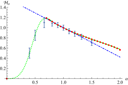
Figure 1: Comparison of the numerical data of Ref. [16] (red dots), interpolation (green solid line), tentatively continued to $\alpha=0$ (green dashed line) and our order-$\varepsilon$ result (blue, dot-dashed). The gray-blue data points with error bars are our numerical estimates for ${\cal H}_{\alpha}$, based on Eq. (14), see D for details.

A major challenge remains, namely evaluation of Pickands’ constant. Only the cases where fBm reduces to standard Brownian motion ($\alpha=1$), and where fBm is an affine process ($\alpha=2$, i.e. a straight line) are known,

$${\cal H}_{1}=1\qquad\textrm{ and }\qquad{\cal H}_{2}=\frac{1}{\sqrt{\pi}}\ .$$ (9)

There is yet no analytical result for other values of $\alpha$. In this letter, we use a path integral formulation, evaluated perturbativly around Brownian motion, to show that

$${\cal H}_{\alpha}=1-\gamma_{\rm E}(\alpha-1)+{\cal O}(\alpha-1)^{2}\ ,$$ (10)

where $\gamma_{\rm E}$ is Euler’s constant.

For other values of $\alpha$, only numerical estimations exist, see figure 1. These are difficult, since statistical fluctuations in Pickands’ definition (6) are large. E.g. for a Brownian the estimator (6) convergences as $1/\sqrt{T}$ [16]. A representation with a much better convergence has been given by Dieker and Yakir [16]:

Theorem (Dieker and Yakir, 2014):

$${\cal H}_{\alpha}=\lim_{T\to\infty}\mathbb{E}\!\left(\frac{\rme^{\max_{0<t<T}\chi_{t}}}{\int_{0}^{T}\rme^{\chi_{t}}\rmd t}\right)\ .$$ (11)

Thus effectively the inverse of $T=\mathbb{E}\left(\int_{0}^{T}\rme^{\chi_{t}}\,\rmd t\right)$ can be moved inside the expectation value $\mathbb{E}\left(\rme^{\max_{0<t<T}\chi_{t}}\right)$. The estimator (11) converges much better than Pickands original one, leading to the results presented on figure 1 (red dots).

Let us conclude this introduction by another remarkable theorem due to V.I. Piterbarg [7, 8], which extends Pickands’ theorem by relaxing the stationarity hypothesis. Suppose that a random process $X_{t}$ with zero mean is defined on the interval $[0,T]$, and has a unique time $t_{0}\in(0,T)$ of maximal variance, normalized to $1$. Further suppose that for some positive $a$, $c$, $\alpha$ and $\beta$ the variance and covariance functions satisfy

$$~{}~{}\sigma(t) := \sqrt{\mathbb{E}(X_{t}^{2})}\;=1-a|t-t_{0}|^{\beta}\qquad~{}~{}\mbox{for }t\to t_{0}\ ,$$ (12)

$$r(t,s) := \mathbb{E}\left(X_{t}X_{s}\right)=1-c|t-s|^{\alpha}\quad\mbox{for }~{}t\to t_{0}\mbox{ and }s\to t_{0}\ .$$ (13)

One finally needs a weak regularity condition, namely that for some $\gamma$ and $G$ positive, $\mathbb{E}\left(X_{t}-X_{s}\right)^{2}\leq G|t-s|^{\gamma}$. The theorem D.3 of Piterbarg [7] (see also [8]) then distinguishes several cases. We only state the one which is relevant below.

Theorem (Piterbarg 1978):

If $\beta>\alpha$, then

$$\qquad\mathbb{P}\!\left(\max\limits_{t\in[0,T]}X_{t}>u\right)=\frac{2{\cal{\cal H}_{\alpha}}\Gamma(1+1/\beta)c^{\frac{1}{\alpha}}}{a^{\frac{1}{\beta}}}u^{\frac{2}{\alpha}-\frac{2}{\beta}}\Psi(u)~{}~{}\mbox{ as }u\to\infty\ ,$$ (14)

with ${\cal H}_{\alpha}$ and $\Psi(u)$ as defined in Eqs. (5) and (6).

This beautiful theorem applies to a fractional Brownian bridge defined on $[0,1]$ and reproduces the Pickands constant of Eq. (10), see D.

To simplify the discussion in the next sections, we introduce a process $z_{t}$ with an arbitrary drift strenght $\mu$

$$z_{t}=B_{t}+\mu|t|^{\alpha}\ .$$ (15)

Setting $\mu=-1$ allows us to recover $z_{t}=\chi_{t}$, as defined in Eq. (8). Pickands’ constant can also be computed by setting $\mu=1$, using

$$\mathcal{H}_{\alpha}=\lim\limits_{T\to\infty}\frac{1}{T}\mathbb{E}(\rme^{-\min_{t\in[0,T]}z_{t}})\ .$$ (16)

2 Brownian with drift, and its Pickands constant ($\alpha=1$)

We recall some results about Brownian motion with drift which are useful to expand Pickands’ constant around $\alpha=1$.

For $\alpha=1$, the fBm process $B_{t}$ is a standard Brownian motion, with covariance $\mathbb{E}(B_{t}B_{s})=2D\min(t,s)$, and diffusion constant $D$. The propagator $P^{+}_{\mu}$ of the process $z_{t}$ defined in Eq. (15), with positivity constraint is

$$P^{+}_{\mu}(x_{0},x,T) := \,\partial_{x}\mathbb{P}\!\left(z_{T}<x,\min\limits_{t\in[0,T]}z_{t}>0\,\Big{|}z_{0}=x_{0}\right)$$ (17)

$$= \,\frac{\rme^{\frac{\mu}{2D}(x-x_{0})-\frac{\mu^{2}}{4D}T}}{\sqrt{4\pi DT}}\!\left(\rme^{-\frac{(x-x_{0})^{2}}{4DT}}-e^{-\frac{(x+x_{0})^{2}}{4DT}}\right)$$

$$= \,\rme^{\frac{\mu}{2D}(x-x_{0})-\frac{\mu^{2}}{4D}T}P_{0}^{+}(x_{0},x,T)\ .$$

Here $P_{0}^{+}$ is the propagator for the process without drift, i.e. $\mu=0$. To compute Pickands’ constant we choose $\mu=D=1$, cf. Eq. (16). We can recover a generic diffusion constant $D$ (with $\mu=D$), by setting $T\to DT$ as can be checked on Eq. (17). The survival probability $Q$ of this process, which is defined as the probability to remain positive up to time $T$ while starting at $x_{0}>0$, can be computed from $P_{\mu}^{+}$ as

$$Q_{\alpha=1}(x_{0},T)=\int_{0}^{\infty}\!\!\!\rmd x\,P^{+}_{\mu=1}(x_{0},x,T)=\frac{1}{2}\!\left[\mbox{erf}\!\left(\frac{x_{0}+T}{2\sqrt{T}}\right)-\rme^{-x_{0}}\mbox{erfc}\!\left(\frac{x_{0}-T}{2\sqrt{T}}\right)+1\right].$$

From this result we can extract the distribution of $m$, defined as $m:=-\min_{t\in[0,T]}z_{t}$,

$$\qquad\mathcal{P}^{T}_{\alpha=1}(m)=\partial_{m}Q_{\alpha=1}(m,T)=\frac{1}{2}\rme^{-m}\mbox{erfc}\left(\frac{m-T}{2\sqrt{T}}\right)+\frac{\rme^{-\frac{(m+T)^{2}}{4T}}}{\sqrt{\pi T}}\ .$$ (19)

The result (19) allows us to compute Pickands’ constant via its main definition (16):

$$\int_{0}^{\infty}\!\!\!\rmd m\,e^{m}\mathcal{P}^{T}_{\alpha=1}(m)=\left(\frac{T}{2}+1\right)\!\left[\mathrm{erf}\!\left(\frac{\sqrt{T}}{2}\right)+1\right]+\sqrt{\frac{T}{\pi}}e^{-\frac{T}{4}}$$

$$\hphantom{\int_{0}^{\infty}\!\!\!\rmd m\,e^{m}\mathcal{P}^{T}_{\alpha=1}(m)}\!\!\stackrel{{\scriptstyle T\to\infty}}{{\simeq}}T+2+\mathcal{O}(e^{-\frac{T}{4}}).$$ (20)

The Pickands constant is the coefficient of the linear term in the large-$T$ asymptotics of Eq. (2). We thus recover the known result for the Brownian, $\mathcal{H}_{1}=1$.

3 Perturbative expansion around Brownian motion: $\alpha=1+2\varepsilon$

3.1 Action

For

$$\alpha=1+2\varepsilon$$ (21)

with $\varepsilon$ a small parameter, we construct in A the action for the process $z_{t}$, defined in Eq. (15) with $\mu=1$. This follows the ideas of [17, 18, 19, 20]. One writes

$$\mathcal{S}[z_{t}]=\mathcal{S}_{0}[z_{t}]+\varepsilon\,\mathcal{S}_{1}[z_{t}]+\mathcal{O}(\varepsilon^{2})\ ,$$ (22)

with

$$\qquad\mathcal{S}_{0}[z_{t}]= \int_{0}^{T}\rmd t\,\frac{\dot{z}_{t}^{2}}{4D_{\varepsilon,\tau}}-\frac{(z_{T}-z_{0})}{2}+\frac{D_{\varepsilon,\tau}T}{4}\ ,$$ (23)

$$\qquad\mathcal{S}_{1}[z_{t}]= -\frac{1}{2}\int_{0}^{T}\rmd t\,\dot{z}_{t}\ln\!\left(\frac{t}{T-t}\right)-\frac{1}{2}\int_{0}^{T-\tau}\!\!\!\rmd t_{1}\int_{t_{1}+\tau}^{T}\!\!\rmd t_{2}\,\frac{\dot{z}_{t_{1}}\dot{z}_{t_{2}}}{t_{2}-t_{1}}\ .~{}~{}~{}~{}~{}~{}~{}~{}$$ (24)

We recognise $\mathcal{S}_{0}$ as the standard Brownian action with a diffusion constant [20]

$$D_{\varepsilon,\tau}=1+2\varepsilon[1+\ln(\tau)]+\mathcal{O}(\varepsilon^{2})\ ,$$ (25)

and a linear drift $\mu=D_{\varepsilon,\tau}$. The time $\tau$ is a regularization cutoff for coinciding times (an UV cutoff), necessary to define perturbation theory. It has no impact on the distribution of observables which can be extracted from the path integral [18, 20].

3.2 Pickands’ constant

To investigate Pickands’ constant, we start with a path-integral representation for the survival probability of the process $z_{t}$, an idea introduced in Refs. [21, 22], and developed for the situation at hand in Refs. [18, 17, 20, 19]:

$$Q_{\alpha}(m,T)=\frac{1}{Z^{\rm N}(T)}\int_{0}^{\infty}\rmd x\int_{z_{0}=m}^{z_{T}=x}\mathcal{D}[z_{t}]\,\Theta[z_{t}]\rme^{-\mathcal{S}[z_{t}]}\ ,$$ (26)

where $\Theta[z_{t}]$ constrains the path $z_{t}$ to remain positive; the normalisation constant $Z^{\rm N}(T)$ is the sum over all paths without the constraint $z_{0}=m$ (and thus independent of $m$). Computing the path integral in Eq. (26) within the $\varepsilon$-expansion of the action (22) allows us to write

$$Z^{\rm N}(T)Q_{\alpha}(m,T) = Z_{0}^{+}(m,T)+\varepsilon Z_{1}^{+}(m,T)+\mathcal{O}(\varepsilon^{2})$$

$$= \langle\Theta[z_{t}]\rangle_{0}+\varepsilon\!\left[\langle\Theta[z_{t}]\mathcal{S}_{1}[z_{t}]\rangle_{0}+2(1+\ln\tau)T\partial_{T}Z_{0}^{+}(m,T)\right]+\mathcal{O}(\varepsilon^{2})\ .$$

The symbol $\langle...\rangle_{0}$ denotes averages over paths $z_{t}$ with the standard Brownian action with drift ($\mu=D=1$), initial conditon $z_{0}=m$ and a free end-point $z_{T}$. Thus, the zeroth-order term

$$Z_{0}^{+}(m,T)\equiv\langle\Theta[z]\rangle_{0}\equiv Q_{\alpha=1}(m,T)$$ (28)

is the survival distribution of the Brownian as given in Eq. (2). For the order-$\varepsilon$ term $Z_{1}^{+}$, there is a contribution due to the non-local correction of the action $\mathcal{S}_{1}$, cf. Eq. (24), and a contribution due to the rescaling of the diffusive constant (and the drift) in $\mathcal{S}_{0}$, $D=1\to D_{\varepsilon,\tau}$.

Before expliciting these terms, we show how this leads to the Pickands constant. Using $Z_{N}(T)=\lim_{m\to\infty}Z_{N}(T)Q_{\alpha}(m,T)$, (note that $Q_{\alpha}$ is the cumulative distribution), we arrive at

$$\qquad Q_{\alpha}(m,T)=Z_{0}^{+}(m,T)[1-\varepsilon\lim\limits_{m\to\infty}Z_{1}^{+}(m,T)]+\varepsilon Z_{1}^{+}(m,T)+\mathcal{O}(\varepsilon^{2})\ .$$ (29)

As for $\alpha=1$ in Eq. (2), the Pickands constant is obtained from the large-$T$ asymptotics of

$$\int_{0}^{\infty}\rmd m\,e^{m}\partial_{m}Q_{\alpha}(m,T)=\int_{0}^{\infty}\rmd m\,e^{m}\partial_{m}Z_{0}^{+}(m,T)$$ (30)

$$+\,\varepsilon\left[\int_{0}^{\infty}\rmd m\,e^{m}\partial_{m}Z_{1}^{+}(m,T)-\lim\limits_{m\to\infty}Z_{1}^{+}(m,T)\int_{0}^{\infty}\rmd m\,e^{m}\partial_{m}Z_{0}^{+}(m,T)\right]+\mathcal{O}(\varepsilon^{2})\ .$$

The first term was already computed in Eq. (2). For the order-$\varepsilon$ term, the function $Z_{1}^{+}(m,T)$ can be expressed from the bare propagator $P_{\mu=1}^{+}$, given in Eq. (17), and its cumbersome Laplace transform $\tilde{Z}_{1}^{+}(m,s)$ derived in B. The asymptotics

$$\int_{0}^{\infty}\!\!\!\rmd m\,e^{m}\partial_{m}Z_{1}^{+}(m,T)\stackrel{{\scriptstyle T\to\infty}}{{=}}\frac{T^{2}}{2}\!\left[\ln\!\left(\frac{T}{\tau}\right)-1\right]+{T}\!\left[\ln\!\left(\frac{T}{\tau}\right)-1-2\gamma_{\rm E}\right]+\mathcal{O}\big{(}\ln(T)\big{)}$$

and

$$\lim\limits_{m\to\infty}Z_{1}^{+}(m,T)=\frac{T}{2}\left[\ln\!\left(\frac{T}{\tau}\right)-1\right]\ ,$$ (32)

allows us to compute Pickands’ constant at order $\varepsilon$. Combining these contributions according to Eq. (30) cancels the $\tau$ dependence, as it should, and finally gives

$$\mathcal{H}_{1+2\varepsilon}=1-2\varepsilon\gamma_{\rm E}+\mathcal{O}(\varepsilon^{2})\equiv 1-(\alpha-1)\gamma_{\rm E}+\mathcal{O}\!\left(\alpha-1\right)^{2}\ ,$$ (33)

where $\gamma_{\rm E}$ is the Euler-Mascheroni constant, whose numerical value is $\gamma_{\rm E}\approx 0.577$.

This result, which gives the derivative of the Pickands constant at $\alpha=1$, compares favourably to the extensive numerical simulations of Ref. [16] plotted on figure 1. Though much less precise, it is also in agreement with our results obtained by numerical simulations of the maximum of a fBm bridge, using Eqs. (14)–(63).

3.3 Distribution of $m$ at large $T$

For standard Brownian motion, $\alpha=1$, the distribution $\mathcal{P}_{\alpha=1}^{T}(m)$ given in Eq. (19) has the interesting property to converge to a non-trivial limit when $T\to\infty$, namely

$$\mathcal{P}_{\alpha=1}^{\infty}(m)=\lim\limits_{T\to\infty}\partial_{m}Q_{\alpha=1}(m,T)=\rme^{-m}\ .$$ (34)

Using the same expansion as in Eq. (30), we can express this distribution for $\alpha=1+2\varepsilon$,

$$\mathcal{P}_{\alpha}^{T}(m)=\partial_{m}Z_{0}^{+}(m,T)+\,\varepsilon\left[\partial_{m}Z_{1}^{+}(m,T)-\Big{(}\lim\limits_{m\to\infty}Z_{1}^{+}(m,T)\Big{)}\partial_{m}Z_{0}^{+}(m,T)\right]+\mathcal{O}(\varepsilon^{2})\ .$$

The expression of $\tilde{Z}_{1}^{+}(m,s)$ given in B encodes $\mathcal{P}_{\alpha}^{T}(m)$ for a generic $T$, but we restrict ourselves to the large-$T$ limit for simplicity. Using the asymptotics

$$\partial_{m}Z_{1}^{+}(m,T)\stackrel{{\scriptstyle T\to\infty}}{{=}}-2\rme^{-m}\left\{1+\gamma_{\rm E}+\ln(m)+\frac{T}{4}\!\left[1+\ln\!\left(\frac{\tau}{T}\right)\right]\right\}-2\mbox{Ei}(-m)+\mathcal{O}\Big{(}\frac{1}{T}\Big{)},$$

and the one given in Eq. (32), we see that $\mathcal{P}_{\alpha}^{T}(m)$ converges at large $T$ to a non-trivial distribution,

$$\qquad\mathcal{P}_{\alpha=1+2\varepsilon}^{\infty}(m)=\rme^{-m}\Big{\{}1-2\varepsilon\big{[}1+\gamma_{\rm E}+e^{m}\mbox{Ei}(-m)+\ln(m)\big{]}\Big{\}}+\mathcal{O}(\varepsilon^{2})\ .$$ (37)

This is in agreement with the following conjecture: For all $\alpha\in(0,2)$, the distribution $\mathcal{P}_{\alpha}^{T}(m)$ converges to a distribution $\mathcal{P}_{\alpha}^{\infty}$(m) which has the large-$m$ asymptotics

$$\mathcal{P}_{\alpha}^{\infty}(m)\stackrel{{\scriptstyle m\to\infty}}{{\simeq}}\frac{\mathcal{H}_{\alpha}}{\alpha}m^{\frac{1}{\alpha}-1}\rme^{-m}\ .$$ (38)

This conjecture is numerically tested on figure 2. It can be motivated heuristically, see C.

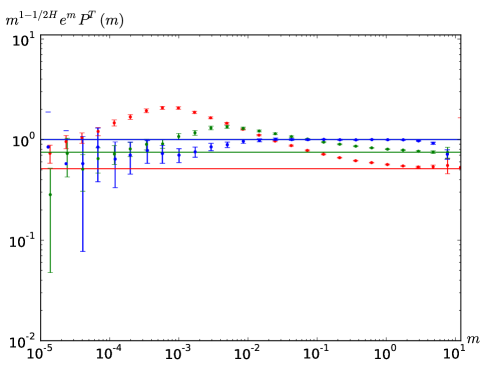
Figure 2: Test on the asymptotic behavior of $\mathcal{P}_{\alpha}^{\infty}(m)$, for $\alpha=1.$ (blue), $\alpha=1.2$ (green) and $\alpha=1.5$ (red). Plain lines represent the conjectured limits for large $m$, using the numerical value of $\mathcal{H}_{\alpha}$ from [16]. Simulation parameters are $T=8$, $dt=2^{-14}$, with $10^{6}$ samples.

4 Conclusions

In this letter, we derived the linear term in the expansion of the Pickands constant around Brownian motion. Apart from the Pickands constant at $\alpha=1$ and $\alpha=2$, this is the only analytically available information we have today.

It would be interesting to continue this approach to higher orders. While the quadratic term seems feasible, it is rather difficult to evaluate, and has to be left for future research.

As our methods allow us to obtain the full distribution of the maximum, and not only its limiting behavior for large arguments, other questions can be posed. A particularly interesting one is the probability distribution of the maximum of a fBm with an unconstraint endpoint. From [7, 8] we know that at $\alpha=1$ this behavior changes. For $\alpha<1$ it is non-trivial as in Eq. (14), while for $\alpha>1$ the tail is simply given by the distribution at the endpoint. For $\alpha$ close to 1 both terms will contribute in a non-trivial way yet to be determined.

Aaknowledgments

We thank V.I. Piterbarg, S. Kobelkov, S.N. Majumdar, K. Mallick and W. Werner for helpful discussions. Part of this work has been supported by PSL through grant ANR-10-IDEX-0001-02-PSL.

Appendix A Derivation of the action in presence of a drift

Here we derive the action for the process $z_{t}=B_{t}+\mu\,t^{\alpha}$, where $X_{t}$ is a fractional Brownain motion, close to standard Brownian motion, i.e. with parameter $\alpha=1+2\varepsilon$, and $\varepsilon$ small. As the process $B_{t}$ is Gaussian, its action is given by its covariance function $G^{-1}(t_{1},t_{2})=\mathbb{E}(B_{t_{1}}B_{t_{2}})$,

$$\mathcal{S}[B]=\frac{1}{2}\int_{t_{1},t_{2}}\dot{B}_{t_{1}}G(t_{1},t_{2})\dot{B}_{t_{2}}\ .$$ (39)

While it is not possible to derive a simple closed expression for a generic value of $\alpha$, we can express the action $\mathcal{S}$ in an $\varepsilon$-expansion. This was done in Ref. [18] for the process without drift; the result reads

$$\mathcal{S}[B]=\int_{0}^{T}\!\!\rmd t\,\frac{\dot{B}_{t}^{2}}{4D_{\varepsilon,\tau}}-\frac{\varepsilon}{2}\int_{0}^{T-\tau}\!\!\rmd t_{1}\int_{t_{1}+\tau}^{T}\!\!\rmd t_{2}\,\frac{\dot{B}_{t_{1}}\dot{B}_{t_{2}}}{t_{2}-t_{1}}+\mathcal{O}(\varepsilon^{2})\ .$$ (40)

The first term involves a rescaled diffusion constant $D_{\varepsilon,\tau}=1+2\varepsilon(1+\ln\tau)+\mathcal{O}(\varepsilon^{2})$. From this, it is possible to obtain the action for $z_{t}$ by changing variables $\dot{B}_{t}\to\dot{z}_{t}-\mu\left[1+2\varepsilon(1+\ln t)\right]+\mathcal{O}(\varepsilon^{2})$. Expanding each term of the action, we get

$$\int_{0}^{T}\!\!\rmd t\,\frac{\dot{B}_{t}^{2}}{4D_{\varepsilon,\tau}} \to \int_{0}^{T}\!\!\rmd t\,\frac{\dot{z}_{t}^{2}}{4D_{\varepsilon,\tau}}-\mu\frac{z_{T}-z_{0}}{2D_{\varepsilon,\tau}}+\frac{\mu^{2}T}{4D_{\varepsilon,\tau}}$$ (41)

$$-\varepsilon{\mu}\int_{0}^{T}\!\!\rmd t\,\dot{z}_{t}(1+\ln t)+\varepsilon{\mu^{2}T\ln(T)}+\mathcal{O}(\varepsilon^{2})\ ,$$

and

$$\int_{0}^{T-\tau}\!\!\rmd t_{1}\int_{t_{1}+\tau}^{T}\!\!\rmd t_{2}\,\frac{\dot{B}_{t_{1}}\dot{B}_{t_{2}}}{t_{2}-t_{1}} \to \int_{0}^{T-\tau}\!\!\rmd t_{1}\int_{t_{1}+\tau}^{T}\!\!\rmd t_{2}\,\frac{\dot{z}_{t_{1}}\dot{z}_{t_{2}}}{t_{2}-t_{1}}-\mu^{2}T\left[\ln\!\left(\frac{\tau}{T}\right)+1\right]$$ (42)

$$-\mu\int_{0}^{T}\rmd t\,\dot{z}_{t}\left[\ln\!\left(\frac{t}{\tau}\right)+\ln\!\left(\frac{T-t}{\tau}\right)\right]+\mathcal{O}(\varepsilon)\ .$$

There are some simplifications:

$$\mu^{2}\frac{T}{4D_{\varepsilon,\tau}}+\varepsilon{\mu^{2}T\ln(T)}+\varepsilon\frac{\mu^{2}T}{2}\left[\ln\!\left(\frac{\tau}{T}\right)+1\right]=\mu^{2}\frac{T^{1+2\varepsilon}}{4}+\mathcal{O}(\varepsilon^{2})$$ (43)

$$\int_{0}^{T}\!\!\!\!\rmd t\,\dot{z}_{t}\ln\!\left(\frac{t(T-t)}{\tau^{2}}\right)-2\int_{0}^{T}\!\!\!\!\rmd t\,\dot{z}_{t}(1+\ln t)=\int_{0}^{T}\!\!\!\!\rmd t\,\dot{z}_{t}\ln\!\left(\frac{T-t}{t}\right)-2(z_{T}-z_{0})(1+\ln\tau)$$

After recombining these terms, we obtain the rather compact expression

$$\mathcal{S}[z_{t}]= \int_{0}^{T}\rmd t\,\frac{\dot{z}_{t}^{2}}{4D_{\varepsilon,\tau}}-\mu\frac{z_{T}-z_{0}}{2}+\mu^{2}\frac{T^{1+2\varepsilon}}{4}$$ (45)

$$-\mu\frac{\varepsilon}{2}\int_{0}^{T}\rmd t\,\dot{z}_{t}\ln\!\left(\frac{t}{T-t}\right)-\frac{\varepsilon}{2}\int_{0}^{T-\tau}\!\!\!\rmd t_{1}\int_{t_{1}+\tau}^{T}\!\!\rmd t_{2}\,\frac{\dot{z}_{t_{1}}\dot{z}_{t_{2}}}{t_{2}-t_{1}}+\mathcal{O}(\varepsilon^{2})\ .$$

The last term of the first line does not depend on $z_{t}$, thus acts as a global normalisation which has no impact on the observables we compute from this action. We choose to change it to $\mu^{2}TD_{\varepsilon,\tau}/4$ for simplicity and fix $\mu=1$, which finally gives the expressions (22) and (23) of the main text.

Appendix B Details of the calculations

In this appendix, we give the details of the computation for the order-$\varepsilon$ correction in the path integral (26). The difficult contribution in Eq. (3.2) is $Z_{1,AB}^{+}:=\langle\mathcal{S}_{1}[z_{t}]\Theta[z_{t}]\rangle_{0}$, which we now decompose into two terms $Z_{1,AB}^{+}=Z_{1A}^{+}+Z_{1B}^{+}$ using the expression of $\mathcal{S}_{1}$ given in the action (23):

$$Z^{+}_{1A}(m,T)=\frac{1}{2}\int_{0}^{T-\tau}\rmd t_{1}\int_{t_{1}+\tau}^{T}\rmd t_{2}\frac{\left\langle\dot{z}_{t_{1}}\dot{z}_{t_{2}}\Theta[z]e^{\frac{Z_{T}-Z_{0}}{2}-\frac{T}{4}}\right\rangle_{0}}{t_{2}-t_{1}}\ ,$$ (46)

and

$$Z^{+}_{1B}(m,T)=\frac{1}{2}\int_{0}^{t}\rmd t\left\langle\dot{z}_{t}\,\Theta[z]e^{\frac{Z_{T}-Z_{0}}{2}-\frac{T}{4}}\right\rangle_{0}\ln\left(\frac{t}{T-t}\right)\ .$$ (47)

The averages $\langle...\rangle_{0}$ denote averages with respect to the standard Brownian action, with no drift, as the drift is now enforced by the exponential factors. We can express these averages in terms of the drift-free bare propagator with positivity constraint, $P_{0}^{+}$. Following the diagrammatic rules defined in Ref. [23], the first correction can be written after a Laplace transform $T\to s$ as

$$\tilde{Z}_{1A}^{+}(m,s)=2\int_{x_{i},y>0}\!\!\!e^{\frac{x_{3}-m}{2}}\tilde{P}_{0}^{+}\!\left(m,x_{1},\bar{s}\right)\partial_{x_{1}}\tilde{P}_{0}^{+}\!\left(x_{1},x_{2},\bar{s}+y\right)\partial_{x_{2}}\tilde{P}_{0}^{+}\!\left(x_{2},x_{3},\bar{s}\right)\ .$$ (48)

We introduced $\bar{s}:=s+1/4$, a shifted Laplace variable due to the term $e^{-T/4}$. As explained in Ref. [18], each $\dot{z}_{t_{i}}$ in (46) corresponds to a factor of $2\partial_{x_{i}}$ acting to the following propagator in Eq. (48). To account for the factor of $(t_{2}-t_{1})^{-1}$, we use the identity $(t_{2}-t_{1})^{-1}=\int_{y>0}e^{-y(t_{2}-t_{1})}$ which produces a shift in the second propagator by a new variable $y$ wkich we need to integrate over. We recall the expression of the propagator in Laplace variables,

$$\tilde{P}_{0}^{+}(x_{1},x_{2},s)=\frac{e^{-\sqrt{s}|x_{1}-x_{2}|}-e^{-\sqrt{s}(x_{1}+x_{2})}}{2\sqrt{s}}\ .$$ (49)

The second correction, due to the non linearity in the drift, is given by

$$Z^{+}_{1B}(m,T)=\int\limits_{x_{i}>0}\!\!\int_{0}^{T}\!\!\!\rmd t\,e^{\frac{x_{2}-m}{2}}P_{0}^{+}(m,x_{1},t)\partial_{x_{1}}P_{0}^{+}(x_{1},x_{2},T-t)\ln\!\left(\frac{t}{T-t}\right)e^{-\frac{T}{4}}\ .$$

In order to compute its Laplace transform, we use the integral representation

$$\ln\!\left(\frac{t}{T-t}\right)=\int_{0}^{\infty}\frac{\rmd y}{y}\left(e^{-y(T-t)}-e^{-yt}\right)\ .$$ (51)

Inserting this into Eq. (B) and taking the Laplace transform gives

$$\tilde{Z}_{1B}^{+}(m,s) = \int_{0}^{\infty}\frac{\rmd y}{y}\int_{x_{i}>0}e^{\frac{x_{2}-m}{2}}\Big{[}\tilde{P}_{0}^{+}(m,x_{1},\bar{s})\,\partial_{x_{1}}\tilde{P}_{0}^{+}(x_{1},x_{2},\bar{s}+y)$$ (52)

$$~{}~{}~{}~{}~{}~{}~{}~{}~{}~{}~{}~{}~{}~{}~{}~{}~{}~{}~{}~{}~{}~{}~{}~{}~{}~{}~{}~{}-\tilde{P}_{0}^{+}(m,x_{1},\bar{s}+y)\,\partial_{x_{1}}\tilde{P}_{0}^{+}(x_{1},x_{2},\bar{s})\Big{]}\ .$$

For both $\tilde{Z}_{1A}^{+}$ and $\tilde{Z}_{1B}^{+}$, the integrals over the space variables $x_{i}$ can be computed quite easily, as the Laplace-transformed propagator $\tilde{P}_{0}^{+}$ is exponential in these variables (contrary to the time-dependent propagators, where the dependence is Gaussian). For the integral over $y$, $\tilde{Z}_{1A}^{+}$ has a logarithmic divergence at large $y$ which corresponds to the UV divergence when $t_{2}\to t_{1}$ in Eq. (46). The necessary large-$y$ cutoff $\Lambda$ (such that the integration over $y$ is performed in the interval $[0,\Lambda]$) equivalent to the UV cutoff $\tau$ is given by $\Lambda=e^{-\gamma_{\rm E}}/\tau$, .

Combining these two terms finally gives (remind $\bar{s}=s+\frac{1}{4}$)

$$s^{2}\Big{[}\tilde{Z}_{1A}(m,s)+\tilde{Z}_{1B}(m,s)\Big{]}$$ (53)

$$= -\frac{e^{\left(\sqrt{\bar{s}}-\frac{1}{2}\right)m}}{8\sqrt{\bar{s}}}\Big{[}8\bar{s}^{3/2}(m+1)+8s\bar{s}m+4\bar{s}-2\sqrt{\bar{s}}(m-1)-1\Big{]}\mbox{Ei}\!\left(-2\sqrt{\bar{s}}m\right)$$

$$+\frac{e^{-\left(\sqrt{\bar{s}}+\frac{1}{2}\right)m}}{16\sqrt{\bar{s}}}\bigg{[}\left(8\bar{s}^{3/2}+8s\bar{s}m+4\bar{s}+2\sqrt{\bar{s}}-1\right)\big{(}\ln(4\bar{s}\tau)+1+\gamma_{\rm E}\big{)}-8\sqrt{\bar{s}}$$

$$~{}~{}~{}~{}~{}~{}~{}~{}~{}~{}~{}~{}~{}~{}~{}~{}~{}~{}~{}~{}+\left(8\bar{s}^{3/2}-8s\bar{s}m+4\bar{s}-6\sqrt{\bar{s}}-1\right)\left(\ln\!\left(\frac{m^{2}}{\tau}\right)-1+\gamma_{\rm E}\right)\bigg{]}$$

$$+\frac{1}{2}\Big{[}\mbox{Ei}\!\left(-\frac{m}{2}-m\sqrt{\bar{s}}\right)+e^{-m}\mbox{Ei}\!\left(\frac{m}{2}-m\sqrt{\bar{s}}\right)-\ln(s\tau)-\gamma_{\rm E}\Big{]}\ .$$

From this expression, and denoting $\tilde{Z}_{1AB}^{+}:=\tilde{Z}_{1A}^{+}+\tilde{Z}_{1B}^{+}$ , it is possible to compute the asymptotics used in the main text, first in terms of the Laplace variable:

$$\tilde{Z}_{1AB}(m,s) \stackrel{{\scriptstyle s\to 0}}{{\simeq}} \frac{(e^{-m}-1)[\ln(s\tau)+\gamma_{\rm E}]}{2s^{2}}$$ (54)

$$+2\frac{e^{-m}[\ln(m)+\gamma_{\rm E}]-(m+1)\mbox{Ei}(-m)}{s}+\mathcal{O}\big{(}\ln(s)\big{)}\ ,$$

$$\tilde{Z}_{1AB}(m,s) \stackrel{{\scriptstyle m\to\infty}}{{\simeq}} -\frac{\ln(s\tau)+\gamma_{\rm E}}{2s^{2}}+\mathcal{O}(e^{-m})\ ,$$ (55)

and

$$\int_{0}^{\infty}\!\!\!\rmd m\,e^{m}\partial_{m}\tilde{Z}_{1AB}^{+}(m,s)\stackrel{{\scriptstyle s\to 0}}{{\simeq}}-\frac{\ln(s\tau)+\gamma_{\rm E}-\frac{1}{2}}{s^{3}}-\frac{\ln(s\tau^{3})+3\gamma_{\rm E}+2}{s^{2}}+\mathcal{O}\Big{(}\frac{1}{s}\Big{)}\ .$$

Note that for the last term it is important to compute the integral over $m$ before expanding in $s$.

The remaining order-$\varepsilon$ correction in Eq. (26) is due to a change of the diffusive constant in the Brownian action, from $D=1$ to $D_{\varepsilon,\tau}=1+2\varepsilon(1+\ln\tau)+\mathcal{O}(\varepsilon)$, with the corresponding change in the drift such that the term linear in $z_{t}$ in $\mathcal{S}_{0}$, c.f. Eq. (23), remains unchanged. This change is equivalent to setting $T\to D_{\varepsilon,\tau}T$ in the result for the Brownian, which, as stated in the main text, gives an order-$\varepsilon$ correction of the form

$$Z_{1D}(m,T)=2(1+\ln\tau)T\partial_{T}Z_{0}^{+}(m,T)$$ (57)

in Eq. (3.2), for a total first-order contribution

$$Z_{1}(m,T)=Z_{1AB}(m,T)+Z_{1D}(m,T)\ .$$ (58)

The rescaling term $Z_{1}^{D}(m,T)$ contributes to the Pickands constant with

$$\int_{0}^{\infty}\!\!\!\rmd m\,e^{m}\partial_{m}{Z}_{1D}(m,T)\stackrel{{\scriptstyle T\to\infty}}{{\simeq}}2(1+\ln\tau)T+\mathcal{O}(e^{-T/4})\ .$$ (59)

The inverse Laplace transform of Eq. (B) plus the contribution from (59) gives the result (3.2) of the main text. For the two other terms, the rescaling of the diffusive constant has no impact as

$$\lim\limits_{T\to\infty}T\partial_{T}Z_{0}^{+}(m,T)=\lim\limits_{m\to\infty}T\partial_{T}Z_{0}^{+}(m,T)=0\ .$$ (60)

Finally, formulae (3.3) and (32) are computed directly from (54) and (55) via an inverse Laplace transformation.

Appendix C Heuristic derivation of the conjecture (38)

The heurisitic derivation of our conjecture (38) is as follows: For $m\ll T^{\alpha}$ and $T\gg 1$ we have $\mathcal{P}^{T}_{\alpha}(m)\simeq\mathcal{P}^{\infty}_{\alpha}(m)$, while for $m\gg T^{\alpha}$, up to subleading (power-law and constant) corrections $\mathcal{P}^{T}_{\alpha}(m)\simeq e^{-\frac{(m-T^{\alpha})^{2}}{4T^{\alpha}}}$, since very large values of the maximum are reached towards the end of the time interval. Using that this cutoff function becomes sharp for large $T$, we get

$$\frac{1}{T}\int_{0}^{\infty}\!\!\rmd m\,e^{m}\mathcal{P}_{\alpha}^{T}(m)\simeq\frac{1}{T}\int_{0}^{T^{\alpha}}\!\!\rmd m\,e^{m}\mathcal{P}^{\infty}_{\alpha}(m)\ .$$ (61)

In order to make Pickands’ definition meaningful, the r.h.s. has to become independent of $T$ for large $T$. This implies that the large-$m$ behaviour of $\mathcal{P}^{\infty}_{\alpha}(m)$ is exponentially decaying in $m$ to compensate the $e^{m}$ prefactor. This can still be multiplied by a power law in $m$ times a constant. The unique such possibility is

$$\mathcal{P}^{\infty}_{\alpha}(m)\simeq\frac{\mathcal{H}_{\alpha}}{\alpha}m^{\frac{1}{\alpha}-1}e^{-m}\ ,$$ (62)

as given in Eq. (38).

Appendix D Extracting the Pickands constant from the maximum of a fBm bridge

Theorem (14) applies to a fractional Brownian bridge defined on $[0,1]$. Normalizing the process s.t. $\mathbb{E}(X_{t=1/2}^{2})=1$, Eqs. (12)–(13) are satisfied with

$$\alpha=2H\;,\quad\beta=2\;,\quad a=\frac{4\alpha(2^{1-\alpha}\alpha-\alpha+1)}{4-2^{\alpha}}\;,\quad c=\frac{2^{\alpha+1}}{4-2^{\alpha}}\ .$$ (63)

Expanding Eq. (14) in $\alpha-1$ yields

$$\partial_{u}\mathbb{P}\left(\mbox{max}_{t\in[0,1]}X_{t}>u\right)\simeq{\cal H_{\alpha}}\,u\,\rme^{-\frac{u^{2}}{2}}\Big{\{}1+\Big{[}\ln(4)-4\ln(u)-1\Big{]}\frac{\alpha-1}{2}+{\cal O}(\alpha-1)^{2}\Big{\}}\ .$$

Our result (90) from Ref. [17], valid at order $\alpha-1$, and expanded for large $u$ is

$$\partial_{u}\mathbb{P}\left(\mbox{max}_{t\in[0,1]}X_{t}>u\right)$$

$$~{}~{}\simeq u\,\rme^{-\frac{u^{2}}{2}}\Big{\{}1+\Big{[}\ln(4)-4\ln(u)-1-2\gamma_{{\rm E}}\Big{]}\frac{\alpha-1}{2}+{\cal O}(\alpha-1)^{2}+{\cal O}(u^{-1})\Big{\}}$$ (65)

This identifies ${\cal H_{\alpha}}=1-\gamma_{{\rm E}}(\alpha-1)+{\cal O}(\alpha-1)^{2},$ confirming Eq. (10).

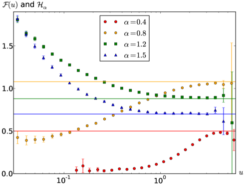
Figure 3: Plot of ${\cal F}(u):=\mathbb{P}\big{(}\max\limits_{t\in[0,1]}X_{t}=u\big{)}u^{1-\frac{2}{\alpha}}\rme^{u^{2}/2}\sqrt{2a}\,c^{-\frac{1}{\alpha}}$, and its convergence to ${\cal H}_{\alpha}$ for $u\to\infty$. The constants $a$ and $c$ are given in Eq. (63). The symbols are simulations for $\alpha=0.4$ to $\alpha=1.5$, cf. legend, with numerical parameters $T/dt=N=2^{18}$ and $10^{6}$ samples. Plain lines of the same color are the estimated asymptotics at large $u$, i.e. the Pickands constant, leading to the gray-blue results presented in Figure 1.

References

- [1] S. N. Majumdar, Universal first-passage properties of discrete-time random walks and Lévy flights on a line: Statistics of the global maximum and records, Physica A 389 (2010) 4299–4316.
- [2] A. J. Bray, S. N. Majumdar and G. Schehr, Persistence and first-passage properties in nonequilibrium systems, Advances in Physics 62 (2013) 225–361.
- [3] B. Derrida and H. Spohn, Polymers on disordered trees, spin glasses, and traveling waves, J. Stat. Phys. 51 (1988) 817–40.
- [4] C. A. Tracy and H. Widom, Level-spacing distributions and the Airy kernel, Comm. Math. Phys. 159 (1994) 151–174, arXiv:hep-th/9211141.
- [5] C. Sire, Probability distribution of the maximum of a smooth temporal signal, Phys. Rev. Lett. 98 (2007) 020601.
- [6] C. Sire, Crossing intervals of non-Markovian Gaussian processes, Phys. Rev. E 78 (2008) 011121.
- [7] V. I. Piterbarg, Asymptotic Methods in the Theory of Gaussian Processes and Fields, Translations of Mathematical Monographs, vol. 148, American Mathematical Society, 1995.
- [8] V. I. Piterbarg, Twenty Lectures About Gaussian Processes, Atlantic Financial Press, 2015.
- [9] A. J. Harper, Pickands’ constant does not equal , for small , arXiv:1404.5505 (2014).
- [10] Z. Michna, Remarks on Pickands theorem, arXiv:0904.3832 (2009).
- [11] K. Dȩbicki and P. Kisowski, A note on upper estimates for Pickands constants, Statist. Probab. Lett. 78 (2008) 2046–2051.
- [12] L. de Haan and J. Pickands, Stationary min-stable processes, Probability Theory and RelatedFields 72 (1986) 477–492.
- [13] J. Pickands III, Asymptotic properties of the maximum in a stationary Gaussian process, Trans. Amer. Math. Soc. 145 (1969) 75.
- [14] C. Borell, The Brunn-Minkowski inequality in Gauss space, Invent. Math. 30 (1976) 207–216.
- [15] B. B. Mandelbrot and J. W. Van Ness, Fractional Brownian motions, fractional noises and applications, SIAM Review 10 (1968) 422–437.
- [16] A. B. Dieker and B. Yakir, On asymptotic constants in the theory of extremes for Gaussian processes, Bernoulli 20 (2014) 1600–1619, arXiv:1206.5840v3.
- [17] M. Delorme and K. J. Wiese, Extreme-value statistics of fractional Brownian motion bridges, arXiv:1605.04132 (2016); Phys. Rev. E. (in print).
- [18] K. J. Wiese, S. N. Majumdar and A. Rosso, Perturbation theory for fractional Brownian motion in presence of absorbing boundaries, Phys. Rev. E 83 (2011) 061141, arXiv:1011.4807.
- [19] M. Delorme and K. J. Wiese, The maximum of a fractional Brownian motion: Analytic results from perturbation theory, Phys. Rev. Lett. 115 (2015) 210601, arXiv:1507.06238.
- [20] M. Delorme and K. J. Wiese, Perturbative expansion for the maximum of fractional Brownian motion, Phys. Rev. E 94 (2016) 012134, arXiv:1603.00651.
- [21] S. N. Majumdar and C. Sire, Survival probability of a Gaussian non-Markovian process: Application to the dynamics of the Ising model, Phys. Rev. Lett. 77 (1996) 1420–1423.
- [22] C. Sire, S. N. Majumdar and A. Rüdinger, Analytical results for random walk persistence, Phys. Rev. E 61 (2000) 1258–1269.
- [23] M. Delorme and K. J. Wiese, unpublished.