A single predator charging a herd of prey: effects of self volume and predator-prey decision-making

Abstract

We study the degree of success of a single predator hunting a herd of prey on a two dimensional square lattice landscape. We explicitly consider the self volume of the prey restraining their dynamics on the lattice. The movement of both predator and prey is chosen to include an intelligent, decision making step based on their respective sighting ranges, the radius in which they can detect the other species (prey cannot recognise each other besides the self volume interaction): after spotting each other the motion of prey and predator turns from a nearest neighbour random walk into direct escape or chase, respectively. We consider a large range of prey densities and sighting ranges and compute the mean first passage time for a predator to catch a prey as well as characterise the effective dynamics of the hunted prey. We find that the prey’s sighting range dominates their life expectancy and the predator profits more from a bad eyesight of the prey than from his own good eye sight. We characterise the dynamics in terms of the mean distance between the predator and the nearest prey. It turns out that effectively the dynamics of this distance coordinate can be captured in terms of a simple Ornstein-Uhlenbeck picture. Reducing the many-body problem to a simple two-body problem by imagining predator and nearest prey to be connected by a Hookean bond, all features of the model such as prey density and sighting ranges merge into the effective binding constant.

1 Introduction

Every animal must eat in order to survive. For certain predator species this necessarily implies to chase and bring down a sufficient amount of prey. With predators always on the lookout for food, prey must constantly be on the alert. While scattering and zigzagging to confuse the predator is a popular method of herd animals to escape [1, 2], if the escape paths are not well co-ordinated individual prey may also block each other. The self volume effect is also relevant in the hunt of killer cells (macrophages, for instance) in biological organisms attacking bacteria colonies or biofilms. In this paper we study the influence of self volume effects on a herd of non-communicating prey with the autonomy of taking decisions on the run, as quantified by the typical time to catch a prey.

In the study of the dynamics of predator-prey systems one is generically interested in the likelihood for the survival of the prey as a function of the parameters of the dynamics of both prey and predator. Prototype mathematical models of predator-prey systems are reaction-diffusion models [3, 4, 5, 6, 7, 8], in which both species are assumed to move randomly. In one dimension the survival probability of a diffusing prey exposed to a number of diffusing predators decays as a power law in time [9, 10]. In two dimensions the predators catch the prey with probability one, but the mean life time of the prey is infinite. The survival probability of a lamb in the presence of $N$ lions in two dimensions decays logarithmically slowly as $\mathscr{S}_{N}(t)\sim\left(\mathrm{ln}t\right)^{-N}$ [10]. In contrast, in dimensions $\geq 3$ the capture is unsuccessful as a consequence of the transience of random walks [11, 12]. Other features considered in predator-prey models include finite life times of the species [13] or the presence of a third party in the form of a repellent obstructing the predator to reach the prey [14]. Moreover, three groups of species hunting each other were modelled [15], owing to the fact that most animal predators are prey of other animals themselves. Finally, effects of safe havens for prey animals may be considered [16].

While such continuum random walk models revealed various interesting results it is clear that the escape and pursuit dynamics is at least partially deterministic, that is, both predator and prey hunt or escape in some sense intelligently. A way to improve the mathematical modelling is to assume that both species can see each other within a certain radius of vision and try to use this as an advantage in the escape and pursuit process [17, 18]. In such a model the motion consists of random walks which turn into directed ballistic transport once predator and prey spot each other. As shown in [17] the probability to escape can be greatly enhanced if the prey can see the predator and has the possibility to run away. During the pursuit the prey’s movement is superdiffusive. In this scenario a total of three predators may be necessary to catch a single prey [17]. Predators may also optimise their search by sharing information [19]. While the assumption of some level of intelligence certainly makes the model more realistic, there is still one aspect that has up to now been ignored. Namely, in reality prey are impenetrable bodies. Thus, in an abundant population of prey (a lion chasing a herd of antelopes, a wolf charging at a flock of sheep, or a killer cell attacking a bacteria colony or biofilm) the prey species may obstruct each other while trying to escape. The self volume (non-phantom) constraint greatly influences the single species and collective dynamics of random walkers [20, 21] leading to qualitative differences in the walkers’ motion. Therefore, the dynamics and survival probability in predator prey systems at intermediate and higher prey densities is expected to be equally affected. Recently a herd of prey chased by a pack of predators including self volume effects was studied [22]. As a result the prey’s survival time was found to increase if the prey aim for a specific type of clustering.

In this paper we study the success of a single predator hunting a flock of prey on a two-dimensional square lattice with periodic boundary conditions taking into account the prey’s self volume. In addition, both species move intelligently in that they can influence their movement by visual perception within their sighting range. The paper is structured as follows: First we introduce our model. Next we present the numerical and analytical results for the mean first capture time, which is the time the predator needs to catch the first prey, as a function of prey density and the respective sighting ranges. We find that the mean first capture time as a function of prey density follows a power law. The (non-universal) exponent depends on the sighting ranges of both predator and prey. For the analytical calculations we split the predator’s motion into a diffusing part and a ballistic part, representing the search for the prey and the direct chase, respectively. We then present a study of the mean distance between predator and nearest prey, which is found to decrease exponentially in time. Using the mean distance we show that we can capture its dynamics in terms of a simple Ornstein-Uhlenbeck process: the relative motion of predator and nearest prey can thus effectively be viewed to be a random process confined by an harmonic potential. Neglecting all other prey, the model parameters such as sighting ranges and prey density can be absorbed into the associated spring constant.

2 Lattice model

To study the success of a single predator hunting a herd of prey we create an agent-based simulation in which predator and prey move on a two dimensional square lattice with periodic boundary conditions. Each species has its specific sighting range $\sigma$ in which it can see the other species as depicted in Fig 1. Distances as well as sighting ranges are measured as chemical distances $d=\Delta x+\Delta y$ of the added bond lengths, with lattice spacing $a$ equal to unity. The predator starts from the centre of the lattice and the prey are initially randomly distributed—excluding the centre of the lattice—such that the occupancy of a single site is less or equal to a single prey. Predators and prey move with the autonomy of decision in the following sense. If no prey is in the sighting range of the predator and, for a given prey, the predator is not in its sighting range, both participants perform a nearest neighbour random walk. If a prey comes into the sighting range of the predator, the predator chooses a site randomly, subject to the condition that the distance $d$ to the prey necessarily decreases. Every lattice site that minimises the distance to the prey is chosen with the same probability, lattice sites that increase the distance cannot be chosen. Analogously, if the predator is spotted the prey chooses a site randomly, subject to the condition that the distance to the predator necessarily increases. If two or more prey are within the same distance to the predator the latter chooses randomly which prey to pursue. Due to the self volume of the prey, the prey’s motion is restricted. In principle, there exist two possible ways to implement the self volume. Either the prey chooses only from empty sites and always executes a jump as long as there is at least one empty nearest neighbour site. Or the prey blindly chooses a nearest neighbour site but only jumps if the chosen site is unoccupied; otherwise, if it is occupied, the prey retains its location. We chose the latter scenario, as this appears closer to the situation encountered for confused prey or for moving bacteria. Using this update strategy, we simultaneously choose the individual moves for the prey and the predator. In each round of motion updates for the prey we randomly choose a sequence of individuals, thus avoiding any bias among individuals [23]. According to this random sequence we then check whether the individual prey are allowed to jump given the actual positions of all other prey. The motion of the predator takes into account the positions of all prey at the end of the previous update. Once all inidividual jumps of prey and predator are determined, all positions of the entire predator-prey system are updated simultaneously.

The time unit is chosen arbitrarily and relates to the diffusion constant $D$

$$\Delta t=\frac{a^{2}}{4D},$$ (1)

where $a=1$ is the lattice spacing. After the individual steps of all participants are accomplished, we check if the predator caught a prey. If the first prey is caught the simulation terminates. The mean first capture time and the mean distance are obtained from $10^{4}$ realisations and the first passage density is obtained from $10^{6}$ runs.

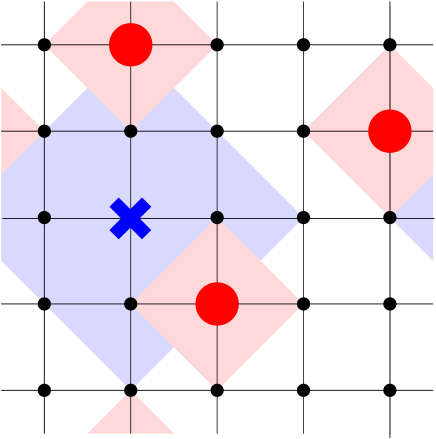
Figure 1: Predator (blue cross) and prey (red dots) on a square lattice. The pale blue and red diamonds represent their respective sighting ranges. Due to their self volume different prey are not allowed to share the same lattice site. Once a prey and the predator meet at the same lattice site the predator is considered to have caught the prey.

3 Mean first capture time

We start by quantifying the success of the predator by computing the mean first capture time $\left\langle\tau_{c}\right\rangle$, that is, the typical time the predator needs to catch the first prey. In mathematical terms this corresponds to the prey’s survival time. As one can easily imagine the mean first capture time depends crucially on both sighting ranges $\sigma_{\mathrm{prey}}$ and $\sigma_{\mathrm{pred}}$ as well as on the prey density $\varrho=N/L^{2}$, where $N$ is the number of prey and $L^{2}$ is the number of lattice sites. A higher prey density reduces the prey’s survival expectation. One reason is that the probability that initially one prey sits close to the predator is higher and therefore the prey gets spotted earlier. The second reason is that a chased prey gets trapped more easily if there are more prey that occupy nearest neighbour sites and therefore lead to a frustration of the prey’s mobility.

In this setup we distinguish two limiting cases: A single prey ($\varrho=1/L^{2}$) with sighting range greater than two can never get caught, its life time is infinite. Conversely, if every lattice spacing is occupied by a prey ($\varrho=1-1/L^{2}$) then the predator needs exactly one time step to catch the first prey. For arbitrary densities, as a result of extensive simulations we find from Fig. 2 that the mean first capture time as a function of the prey density follows a power law behaviour

$$\left\langle\tau_{c}\right\rangle\sim\varrho^{-\beta\left(\sigma_{\mathrm{pred}},\sigma_{\mathrm{prey}}\right)}$$ (2)

in which different combinations of sighting ranges lead to different slopes. Furthermore, there appears a crossover between two regimes for larger sighting ranges of the prey, in which we find different slopes for the low and intermediate density range and the high density range; see, for instance, the square symbols in Figs. 2 b) and c).

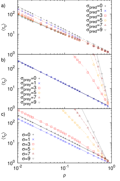
Figure 2: Mean first capture time as a function of the prey density, averaged over $10^{4}$ realisations. a) Blind prey, the predator’s sighting range increases from top to bottom: $\sigma_{\mathrm{pred}}=0,1,3,5,7,9$. b) Blind predator, the preys’ sighting range increases from bottom to top: $\sigma_{\mathrm{prey}}=0,1,3,5,7,9$. c) Identical sighting ranges of prey and predator, sighting ranges increase from bottom to top, $\sigma_{\mathrm{prey}}=\sigma_{\mathrm{pred}}=0,1,3,5,7,9$. The lines are power-law fits according to Eq. (2). The exponent $\beta$ as a function of sighting ranges is depicted in Fig. 10 in B.

In more detail, while the predator’s sighting range only slightly influences the prey’s survival, as shown in Fig. 2a), the prey can increase their life expectancy significantly by a finite sighting range of at least two, compare Fig. 2b), even in the case of a long sighting range of the predator, see Fig. 2c). In both figures 2b) and 2c) a significant variation at intermediate $\sigma$ values is distinct. We note that a short sighting range of the prey ($\sigma_{\mathrm{prey}}=1$) has no advantage over a vanishing one. An explanation can be found “microscopically”. There are two possibilities for a prey to get caught. First, a prey gets stuck and, despite his eyesight, cannot evade the encounter with the predator; or, second, predator and prey simultaneously jump on the same lattice site and collide randomly, see Fig. 3. With sighting range zero or one a prey cannot foresee a random collision, because the distance decreases instantly from two to zero. Thus, the prey needs at least a sighting range of two to prevent such a situation. These random collisions further lead to the fact that the predator is more successful with an even sighting range $\sigma_{\mathrm{pred}}=2n$, $n$ being an integer number, than with a higher odd one $\sigma_{\mathrm{pred}}=2n+1$. Since the random collision is a natural and frequent way to get caught, we decided to eliminate these effects by treating only odd sighting ranges.

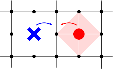
Figure 3: A short-sighted prey ($\sigma_{\mathrm{prey}}$=1), depicted by the red dot, can get caught by the predator (blue cross) despite his field of vision by random collision, due to simultaneous jumps to the same lattice site.

We note that we did not include error bars in our figures. A stochastic variable with exponential (Poissonian) probability density function $p(t)=\tau^{-1}\mathrm{e}^{-t/\tau}$ has the mean $\tau$ and variance $\tau^{2}$. The mean first capture time presented in this section is the first moment of the exponentially distributed first passage density obtained in section 4.3. The standard deviation of this Poissonian process $\sigma=\sqrt{\int_{0}^{\infty}t^{2}p(t)-\tau^{2}\mathrm{d}t}$ is equal to the mean $\tau$, which is indeed confirmed from our numerical results with a sample size of $10^{4}$ per data point. Repeated simulations produced practically indistinguishable results.

4 Distribution of first capture times

In comparison to an ensemble of non-interacting random walkers self volume effects and the autonomy of decision-making of the participants limit the possibilities of analytical calculations. We succeeded in calculating the distribution of the time for catching the first prey only in the case of blind prey. As the results are nevertheless instructive we discuss this case here in some detail. The autonomy to switch the mode of motion of the predator can be included by dividing the process into two subprocesses. The first one describes the diffusing predator while looking out for a prey. The second subprocess portrays the direct chase of the prey, which can in fact be considered as a ballistic motion in chemical space such that the predator still has the option of choosing sites in different directions.

4.1 Searching the prey

The first subprocess describes the random motion of the predator while looking out for a prey. According to the model during that time the predator performs a nearest neighbour random walk on the lattice. We are interested in the first passage density function of the predator to find the first prey, that is, until the first prey enters the predator’s sighting range. For simplification we use a continuous radial coordinate and ignore the fact that the participants move on a lattice. We assume that there exists an effective radius $r_{\mathrm{eff}}$ around the predator in which he will not encounter a prey. This radius has a natural lower bound which is the initial distance between predator and nearest prey (at time $t=0$), calculated in section 5. If the predator hits this effective radius, he spots the prey and will from there on switch his motion to the direct chase calculated in the next subsection.

We consider the predator as a diffusing particle in two dimensions and calculate his first passage time to escape a sphere with radius $r_{\mathrm{\mathrm{eff}}}-\sigma_{\mathrm{pred}}$. For simplification we let the particle diffuse between concentric spheres with an inner reflecting boundary at radius $R_{-}$, which will later tend to zero, and an outer absorbing boundary at radius $R_{+}$, representing the point where the predator spots a prey. $R_{+}$ is thus the distance between predator and prey minus the sighting range of the predator. The predator starts inside the interval $R_{-}<r_{0}<R_{+}$. We will later let $r_{0}$ tend to $R_{-}$ to capture the predator’s starting position correctly. The diffusing particle can be described by the radial diffusion equation

$$\frac{\partial p(r,t)}{\partial t}=D\frac{1}{r^{2}}\frac{\partial}{\partial r}\left(r^{2}\frac{\partial}{\partial r}\right)p(r,t)$$ (3)

for the probability density function $p(r,t)$ to find the predator at radius $r$ at time $t$. The initial condition we choose as $p(r,t=0)=\delta(r-r_{0})/\left(2\pi r_{0}\right)$, that is, the particle starts at $r=r_{0}$. We impose the absorbing boundary condition $p(R_{+},t)=0$ at $R_{+}$ and the reflecting boundary condition $-[\partial p(r,t)/\partial r]_{R_{-}}=0$ at $r=R_{-}$. After Laplace transform

$$\tilde{f}(s)=\mathscr{L}\{f(t)\}(s)=\int\limits_{0}^{\infty}f(t)e^{-st}\mathrm{d}t$$ (4)

and with $x=r\sqrt{s/D}$ the diffusion equation is reduced to the ordinary differential equation

$$\tilde{p}(x,s)-\frac{1}{x}\frac{\partial\tilde{p}(x,s)}{\partial x}-\frac{\partial^{2}\tilde{p}(x,s)}{\partial x^{2}}=\frac{1}{D}\frac{\delta(x-x_{0})}{2\pi x_{0}}$$ (5)

For $x<x_{0}$ and $x>x_{0}$ this is the modified Bessel equation of zero order with known solution $\tilde{p}(x,s)=C_{1}I_{0}(x)+C_{2}K_{0}(x)$ for $x\neq x_{0}$ [24], where $I_{0}(x)$ and $K_{0}(x)$ are the modified Bessel functions of first and second kind. We solve this equation by imposing the continuity condition $\tilde{p}_{<}(x_{0},s)=\tilde{p}_{>}(x_{0},s)$ and the jump-discontinuity

$$\left.-\frac{\partial\tilde{p}_{>}(x,s)}{\partial x}\right|_{x_{0}}+\left.\frac{\partial\tilde{p}_{<}(x,s)}{\partial x}\right|_{x_{0}}=\frac{1}{2\pi Dx_{0}}$$ (6)

where $\tilde{p}_{<}(x,s)$ is the solution in the range $x<x_{0}$ and $\tilde{p}_{>}(x,s)$ is the solution in the range $x>x_{0}$. With the shorthand notations $C_{\nu}(a,b)=I_{\nu}(a)K_{\nu}(b)-K_{\nu}(a)I_{\nu}(b)$ and $D_{\nu,\pm}(a,b)=I_{\nu}(a)K_{\nu\pm 1}(b)+K_{\nu}(a)I_{\nu\pm 1}(b)$ [26] the solution yields in the form

$$\tilde{p}(x,s)=\frac{C_{0}(x,x_{+})}{2\pi Dx_{0}\left(\frac{C_{0}(x_{0},x_{+})C_{-1}(x_{0},x_{-})}{D_{0,-}(x_{0},x_{-})}-D_{-1,+}(x_{0},x_{+})\right)}.$$ (7)

If the particle starts at the inner boundary $r_{0}=R_{-}$, corresponding to $x_{-}$ in the reduced coordinates,

$$\lim_{x_{0}\rightarrow x_{-}}\tilde{p}_{>}(x,s)=-\frac{C_{0}(x,x_{+})}{2\pi Dx_{0}D_{-1,+}(x_{0},x_{+})}$$ (8)

we calculate the flux through the outer boundary as

$$-2\pi x_{+}D\left.\frac{\partial\tilde{p}_{>}(x,s)}{\partial x}\right|_{x_{+}}=\left(x_{-}D_{-1,+}(x_{-},x_{+})\right)^{-1}.$$ (9)

When $x_{-}$ approaches zero, we therefore find that

$$\lim_{x_{-}\rightarrow 0}\tilde{\wp}_{\mathrm{search}}(s)=\left(I_{0}(x_{+})\right)^{-1}=\left(I_{0}\left(R_{+}\sqrt{s/D}\right)\right)^{-1},$$ (10)

where on the right hand side we restored the original variables. This is but the first passage time density function in Laplace space of the predator to spot a prey. From that time the predator will chase the prey directly, this part being calculated in the next subsection.

4.2 Chasing the prey

The second subprocess, which describes the predator’s movement from the moment of spotting the prey until the prey is caught, can be reduced to a one-dimensional problem. Remember that the decision for every step of the predator is constrained by the following rule: the distance to the prey has to necessarily decrease. For the prey, analogously, the goal is to increase the distance. Consequently after a combined predator and prey step the distance between predator and prey can either stay the same or decrease by one lattice spacing if the chosen site of the prey is already occupied and the prey remains at its site. The first capture time can thus be calculated exactly from the number of times a prey remains at its location. A large sighting range of the prey renders the analysis of the chasing process more difficult as all prey try to escape from the predator and will eventually build a cluster that moves away from the predator. Due to the random order of the updates, one cannot say which of the prey remains sitting. Therefore, we confine ourselves to the case of blind prey. In this case the prey undergoes normal diffusion and the predator moves constantly towards the prey. We therefore consider the predator to be a moving cliff towards a diffusing particle, the blind prey. The survival probability of a diffusing particle in presence of a ballistically moving cliff decays exponentially [26],

$$\mathscr{S}(t)\simeq(t/\tau)^{-1/2}e^{-t/\tau}.$$ (11)

The associated first passage density $\wp(t)=-\mathrm{d}\mathscr{S}(t)/\mathrm{d}t$ then becomes

$$\wp_{\mathrm{chase}}(t)\simeq e^{-t/\tau}\left(\frac{(t/\tau)^{-1/2}}{\tau}+\frac{(t/\tau)^{-3/2}}{2\tau}\right).$$ (12)

With the Laplace transform $\tilde{\wp}_{\mathrm{chase}}(s)\sim\left(1+\tau s\right)^{-1/2}$ in the long time limit corresponding to a small $s$ expansion, we finally get $\tilde{\wp}_{\mathrm{chase}}(s)\sim\left(1+\tau s/2\right)^{-1}$.

Using the first passage time densities of the subprocesses of search and chase we calculate the total first capture time density function in the next subsection.

4.3 Density of first capture time

The distribution of the first capture time is now given by the convolution of results $\tilde{\wp}_{\mathrm{search}}(s)=(I_{0}(R_{+}\sqrt{s/D}))^{-1}$ and $\tilde{\wp}_{\mathrm{chase}}(s)\sim\left(1+\tau s/2\right)^{-1}$,

$$\wp(t)=\int_{0}^{t}\wp_{\mathrm{search}}(t^{\prime})\wp_{\mathrm{chase}}(t-t^{\prime})\mathrm{d}t^{\prime}$$ (13)

which designates the probability that the predator spots the first prey at time $t^{\prime}$ and catches the prey during the time span $t-t^{\prime}$. In Laplace space this convolution simplifies to the product $\tilde{\wp}(s)=\tilde{\wp}_{\mathrm{search}}(s)\tilde{\wp}_{\mathrm{chase}}(s)$. The inverse Laplace transform can be obtained in the long time limit, corresponding to taking $s\rightarrow 0$. We thus need to invert

$$\tilde{\wp}(s)\simeq\left(1+(\kappa+\lambda)s+\kappa\lambda s^{2}\right)^{-1},$$ (14)

where $\kappa=R_{+}^{2}/(4D)$ and $\lambda=\tau/2$. Taking the leading terms for small $s$, $\wp(t)\simeq\mathscr{L}^{-1}\left\{\left(1+\Lambda s\right)^{-1}\right\}$ with $\Lambda=\kappa+\lambda$, the inverse Laplace transform yields the final result,

$$\wp(t)\simeq\Lambda^{-1}e^{-t/\Lambda}.$$ (15)

This density of first capture is thus an exponential distribution, where the rate $\Lambda^{-1}$ is a function of the prey density and the predator’s sighting range. Fig. 4 shows the numerical data of our simulation for the case of blind prey and a short sighting range of the predator ($\sigma_{\mathrm{pred}}=1$). The exponential form (15) agrees quite well with the data over the whole density range.

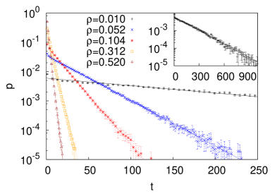
Figure 4: First passage density for the case of blind prey and a short-sighted predator ($\sigma_{\mathrm{pred}}=1$) for different prey densities. Each data point shows the mean result from $10^{6}$ realisations. The error bars were computed from splitting up the $10^{6}$ independent runs into ten runs of $10^{5}$ runs. Inset: Same plot for prey density $\varrho=0.052$ on a larger scale. The lines are exponential fits according to Eq. (15). The exponent $\lambda$ as a function of prey density is depicted in Fig. 9 in B.

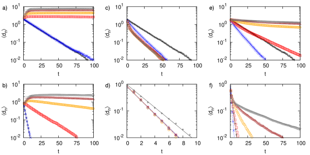
Figure 5: Mean distance between the predator and the nearest prey as function of time, averaged over $10^{4}$ realisations. The upper row (panels a, d, e) shows the case of a low density $\varrho=0.104$ and the lower row (panels b, d, f) represents the case of an intermediate density $\varrho=0.520$. The two left panels a) and b) represent the case of a blind predator, the preys’ sighting range decreases from top to bottom ($\sigma_{\mathrm{prey}}=9,7,5,3,1,0$). The two middle panels c) & d) represent the case of blind prey. The predator’s sighting range increases from top to bottom ($\sigma_{\mathrm{pred}}=0,1,3,5,7,9$). The two panels on the right e) & f) show the mean distance in case of identical sighting ranges ($\sigma_{\mathrm{pred}}=\sigma_{\mathrm{prey}}=0,1,3,5,7,9$). They decrease from top to bottom. The lines are exponential fits according to Eq. (18).

5 Mean distance between predator and nearest prey

We now turn to study the dynamics of the mean distance between the predator and the nearest prey in more detail. In Fig. 5 our simulation results for this mean distance are plotted for a low prey density $\varrho=0.104$ in the upper row (panels a), c) and e)) and for an intermediate density $\varrho=0.520$ in the lower row (panels b), d) and f)). The distance decreases exponentially in time except for the case when a blind predator is combined with a low prey density (Fig. 5 a)) or with a very good eye-sight of the prey (Fig. 5 b)). In these cases the distance is approximately constant in the shown time window. In case of identical sighting ranges the distance between short-sighted species decreases faster than the distance between blind species. This phenomenon is due to the random collisions explained in section 3.

As intuitively expected, the distance between the predator and the nearest prey decreases faster in the case of a large sighting range of the predator. However when the prey’s sighting range is large it softens the decay of the distance. A high prey density also leads to a faster decay of the distance between the predator and the nearest prey, because it implies more prey-prey obstruction events for the chased prey, and with every one such event the distance is reduced by one lattice spacing.

A naive model that captures the effective interaction between two diffusive particles such as the predator and the nearest prey turns out to be the Ornstein-Uhlenbeck process [25]. It is defined in terms of the stochastic differential equation

$$\mathrm{d}x(t)=({\color[rgb]{0,0,1}e}-cx(t))\,\mathrm{d}t+b\,\mathrm{d}W(t)$$ (16)

with non-negative parameters $e$, $b$, and $c$. $W(t)$ denotes the Wiener process [27]. The Ornstein-Uhlenbeck process describes the relaxation of the variable $x$ with initial value $x(t=0)=x_{0}$ to the mean value $e/c$ in the presence of Gaussian white noise. The first moment is given by the exponential decay

$$\left\langle x(t)\right\rangle=\frac{{\color[rgb]{0,0,1}e}}{c}\left[1-\exp(-ct)\right]+x_{0}\exp(-ct).$$ (17)

Comparing the first moment to the observed simulated decay of the mean distance between the predator and the nearest prey (Fig. 5),

$$\left\langle d_{n}\right\rangle\simeq\mathrm{e}^{-\theta t},$$ (18)

we see that the mean distance decreases as a special case of the Ornstein-Uhlenbeck process with vanishing excentricity parameter, $e=0$.

A popular application of the Ornstein-Uhlenbeck process in physics is a Hookean spring with spring constant $k$, whose dynamics is highly overdamped with friction coefficient $\gamma$ in the presence of thermal fluctuations. Therefore we can imagine the predator and the nearest prey to be connected by a Hookean spring and being driven by an external Wiener noise. The corresponding mean relaxes to zero. The equilibrium length of the spring is therefore zero. The bottom of the corresponding harmonic potential thus represents the capture of the prey by the predator. Due to the analogy, the respective sighting ranges and the prey density affect the stiffness of the spring. The spring constant is easily related to the decay rate $\theta$ of the mean distance, $\theta(\varrho,\sigma)=k(\varrho,\sigma)/2$. As shown in Fig. 6 the fitted values for the spring constant display the power law behaviour

$$k\sim\varrho^{\nu}.$$ (19)

The spring constant corresponds to the slopes of the functions in Fig. 5, extracted from the exponential fit and plotted as a function of the prey density. It relates to the mean first capture time discussed in section 3 in the following way. The exponential decay of the mean distance between predator and nearest prey has a mean life time related to the decay rate

$$\tau=\frac{1}{\theta}.$$ (20)

Since the nearest prey is the one that will get caught, its mean first capture time is related to the mean life time of the mean distance and consequently to the inverse of the decay rate, compare Figs. 2 and 6.

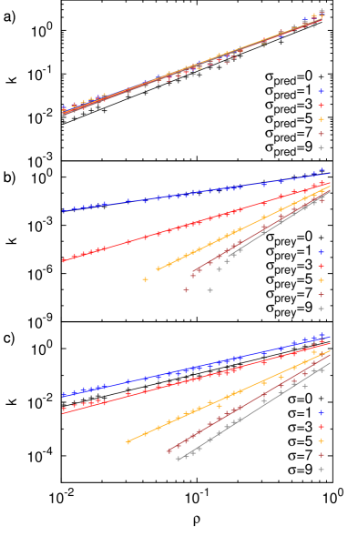
Figure 6: Effective spring constant $k$ of our Ornstein-Uhlenbeck model as function of the prey density for a) blind prey: $\sigma_{\mathrm{pred}}=0,1,3,5,7,9$, increases from bottom to top. b) blind predator: $\sigma_{\mathrm{prey}}=0,1,3,5,7,9$, increases from top to bottom. c) identical sighting ranges: $\sigma_{\mathrm{prey}}=\sigma_{\mathrm{pred}}=0,1,3,5,7,9$, increases from top to bottom. The lines are power law fits according to Eq. (19). The exponent $\nu$ as a function of sighting ranges is depicted in Fig. 10 in B.

Initial distance analysis

We finally mention an analytical approximation for the distance between the predator and the nearest prey. Since we want to capture the whole dynamics we first need to determine the initial distance between predator and nearest prey at time $t=0$. In the simulation we place the predator in the centre and place the prey randomly around him including the self volume interaction. Then we measure the distance between the predator and the nearest prey. In section 4.1 we used an effective radius $r_{\mathrm{\mathrm{eff}}}$ within which the predator does not encounter a prey. Although we cannot calculate this effective radius a natural lower bound is the initial mean distance $\left\langle d_{n}\right\rangle_{t=0}$ between the predator and the nearest prey. Within this distance there is no prey present and therefore it is impossible for the predator to encounter a prey.

We determine the initial distance between the predator and the nearest prey on a square lattice with edge length $L$. The predator sits in the centre of the lattice and the prey are randomly distributed on the remaining $N_{S}=L^{2}-1$ sites. As the prey have a self volume, a lattice site can only be occupied by a single prey. The probability for the distance between predator and nearest prey $d_{n}$ to be equal to $d$ is

$$P(d_{n}=d)=P(d_{n}\geq d)-P(d_{n}\geq d+1).$$ (21)

We then calculate the probability $P(d_{n}\geq d)$ using combinatorics. The detailed calculation can be found in Appendix A. For the probability function of the distance between predator and nearest prey we obtain

$$P(d_{n})=\left[{N_{R}(d)\choose N_{P}}-{N_{R}(d+1)\choose N_{P}}\right]\Big{/}\sum\limits_{i=1}^{d_{\mathrm{max}}}{N_{R}(d_{i})\choose N_{P}},$$ (22)

where we define $d_{\mathrm{max}}$ as the maximal possible distance between the predator and the nearest prey. The expectation value of the initial distance from the predator to the nearest prey, $\left\langle d_{n}\right\rangle=\sum\limits_{d_{i}=1}^{d_{\mathrm{max}}}p(d_{\mathrm{min},i})d_{\mathrm{min},i}$ then yields in the form

$$\left\langle d_{n}\right\rangle=\frac{\sum\limits_{d_{i}=1}^{d_{\mathrm{max}}}d_{i}{N_{R}(d_{i})\choose N_{P}}-{N_{R}(d_{i}+1)\choose N_{P}}}{\sum\limits_{d_{i}=1}^{d_{\mathrm{max}}}{N_{R}(d_{i})\choose N_{P}}-{N_{R}(d_{i}+1)\choose N_{P}}}.$$ (23)

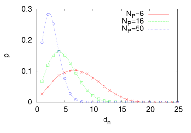
Figure 7: Probability distribution of the initial distance between the predator and the nearest prey for the case of different numbers $N_{P}$ of prey on a square lattice with edge length $L=31$. The crosses represent the numerical data, averaged over $10^{4}$ realisations. The lines show the analytical result (22).

The probability distribution of the initial distance to the nearest prey is shown in Fig. 7 and the related initial mean distance as a function of prey density can be seen in Fig. 8. We simulated both the initial distance distribution and the initial mean distance between the predator and the nearest prey by placing all participants on the lattice under the model conditions with $10^{4}$ iterations. Both analytical and numerical results show excellent agreement in Figs. 7 and 8.

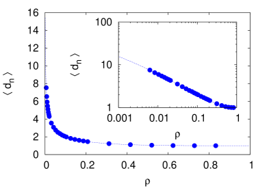
Figure 8: Initial value of the mean distance between the predator and the nearest prey as a function of prey density on a square lattice with edge length $L=31$. The symbols represent the numerical data, averaged over $10^{4}$ realisations, and the dashed line the analytical result (23).

6 Discussion

We studied the predator-prey dynamics of a single predator hunting a herd of prey on a square lattice with decision-making species. While many predator-prey models deal with collective predation [28, 29, 30, 31, 32] or the search for the optimal number of predators given the number of prey [33], we chose a model consisting of one predator and many prey, which is often found in Nature. Solitary hunters such as tigers, bears, or sea turtles often have herd animals as their target. A tiger, for example, hunts a herd of antelopes or a flock of sheep, a bear fishing a salmon out of a swarm, or sea turtles eating jellyfish, shrimp, and fish living in schools. Similarly individual killer cells in biological organisms may attack a colony of bacteria or a biofilm.

A major ingredient of our model is the self volume of the prey, such that no two prey are allowed on a given lattice site. We showed that in the case of impenetrable prey the predator hunts more successfully if the prey have worse eyesight. Moreover, we found that the predator benefits more from a deterioration of the prey’s eyesight than from an improvement of his own eyesight.

While trapping reaction models obtain a minor influence of the prey’s long time survival probability by their diffusion constant [5, 6] we found the prey’s sighting range and thereby motion predominating their survival probability. Due to self volume interactions the prey are forced to improve their eye-sight, and with a good field of vision can drastically increase their chances of survival even in the range of high densities.

The prey only profit from a sighting range of at least two. A very short eyesight does not at all improve its survival probability with respect to being blind. This is attributed to random collisions between predator and prey. Using a simplified analytic approach we showed that in the long time limit the first passage density of the predator to catch a blind prey decays exponentially in time with a non-linear dependence of the decay rate on the prey density.

The effective motion during the chase (described in terms of the distance between the predator and the chased prey) can be effectively described as a linear relaxation process in an harmonic potential with a stochastic driving where the density and sighting ranges determine the stiffness of the corresponding Hookean spring. All non-linear effects entering the motion due to self volume interactions can thus effectively be described with a single parameter.

There exist a range of further open questions. To imitate natural environment one could extend the dynamics by introducing (time or sighting range dependent) waiting times. One could choose different rates of motion for predator and prey as well or even distribute the rates within the prey to simulate old, sick or infant animals. Additionally, many prey live in herds, so one could let the prey be clustered as the initial condition. Last but not least, communication between the prey is a reasonable thing to assume. Once one of the prey spots the predator, immediately all of them are informed (similar to stamping of rabbits or the cheeping calls of groundhogs), that is, a collective response of prey.

We finally note that random search processes with non-Brownian search dynamics are also widely discussed in literature. While Brownian motion is an advantageous process to find nearby targets [34], it is known that pure stochastic motion leads to oversampling of the area on longer time scales. Hence, the optimal number of encounters with prey can be found by switching between search modes [35, 36]. Representative for such a process is for example the intermittent search strategy which combines phases of slow motion, allowing the searcher to detect the target, and phases of fast motion during which targets cannot be detected [37, 38]. Another widely applicable process concerning optimal search strategies are Lévy flights , which are based on random walk processes with long- tailed jump length distributions and are known to be an efficient strategy for finding a target of unknown place [39, 40]. A species which is known to move in Lévy patterns are wandering albatrosses [41, 42] or marine predators as sharks, bony fishes, sea turtles and penguins [43, 44]. It would thus be interesting to study effects of self volume in these models as well.

Appendix A Initial distance between Predator and nearest prey

We determine the initial distance between the predator and the nearest prey on a two dimensional square lattice with edge length $L$. The predator sits in the centre of the lattice and the prey are randomly distributed on the remaining $N_{S}=L^{2}-1$ sites. As the prey have a self volume, a lattice site can only be occupied by a single prey. The probability for the minimal distance between predator and nearest prey $d_{n}$ to be equal to $d$ is

$$P(d_{n}=d)=P(d_{n}\geq d)-P(d_{n}\geq d+1).$$ (24)

We calculate the probability function $p(d_{n}\geq d)$ using combinatorics. If $d_{n}\geq d$ all sites within distance $d$ (up to distance $d-1$) must be unoccupied. To obtain the number of these sites we count all sites at exactly distance $d$ and add them from distance $1$ up to $d-1$. The number of sites at distance $d$ can be shown to be

$$N(d)=\left\{\begin{array}[]{ll}4d,&d\leq(L-1)/2\\ 4(L-d),&d>(L-1)/2\end{array}\right..$$ (25)

Counting all empty sites within the distance $d$ from the predator leads to

$$M(d)=\sum\limits_{i=1}^{d-1}N(i).$$ (26)

That is explicitly,

$$M(d)=\left\{\begin{array}[]{ll}\sum\limits_{i=1}^{d-1}4i=2d(d-1),&d\leq(L+1)/2\\ N_{S}-\sum\limits_{i=1}^{L-d}4i=\left(L^{2}-1\right)-2(L-d)(L-d+1),&d>(L+1)/2\end{array}\right.$$ (27)

Due to the predator sitting in the centre there are in general $N_{S}=L^{2}-1$ possible sites for the prey to be placed on. Under the assumption that the minimal distance is $d$, i.e., $M(d)$ sites are vacant, there are $N_{R}(d)=N_{S}-M(d)$ remaining sites for the prey. The probability for the minimal distance to be greater or equal $d$ is the number of possibilities to place the prey at the remaining sites $N_{R}(d)$ over the possibilities to place the prey at sites greater equal every possible distance ($1$ to $d_{\mathrm{max}}$)

$$P(d_{n}\geq d)={N_{R}(d_{i})\choose N_{P}}\Big{/}\sum\limits_{i=1}^{d_{\mathrm{max}}}{N_{R}(d_{i})i\choose N_{P}}.$$ (28)

For the probability function of $d_{n}$ using Eq. (21) we obtain

$$P(d_{n})=\left({N_{R}(d)\choose N_{P}}-{N_{R}(d+1)\choose N_{P}}\right)\Big{/}\sum\limits_{i=1}^{d_{\mathrm{max}}}{N_{R}(d_{i})\choose N_{P}},$$ (29)

where we define $d_{\mathrm{max}}$ as the maximal possible distance between the predator and the nearest prey. It is determined by the number of prey (due to the self volume of the prey) and can be calculated by allocating all prey as greatest distance as possible starting at $d=L-1$. Then the first fully unoccupied diamond at distance $d$ is the maximal possible distance $d_{\mathrm{max}}$. There exist the following condition to place all prey $N_{P}\leq N_{S}-M(d_{\mathrm{max}})$,

$$\left\{\begin{array}[]{ll}N_{P}\leq\sum\limits_{i=1}^{L-1-d_{\mathrm{max}}}4i,&N_{P}<\frac{N_{S}}{2}\\ N_{P}-\frac{L^{2}-1}{2}\leq\sum\limits_{i=d_{\mathrm{max}}}^{\frac{L-1}{2}}4i,&N_{P}\geq\frac{N_{S}}{2}\end{array}\right..$$ (30)

We then get the maximal possible distance as a function of prey,

$$d_{\mathrm{max}}=\left\{\begin{array}[]{ll}\left\lfloor\frac{2L-1-\sqrt{1+2N_{P}}}{2}\right\rfloor,&N_{P}<N_{S}/2\\[17.07182pt] \left\lfloor\frac{\sqrt{1+2(N_{S}-N_{P})}-1}{2}\right\rfloor,&N_{P}\geq N_{S}/2\end{array}\right.$$ (31)

where $\lfloor x\rfloor:=\max\{m\in\mathbb{Z}\mid m\leq x\}$ is the floor function. We now obtain the expectation value of the initial distance from the predator to the nearest prey,

$$\left\langle d_{n}\right\rangle=\sum\limits_{d_{i}=1}^{d_{\mathrm{max}}}p(d_{\mathrm{min},i})d_{\mathrm{min},i}$$ (32)

such that

$$\left\langle d_{n}\right\rangle=\frac{\sum\limits_{d_{i}=1}^{d_{\mathrm{max}}}d_{i}{N_{R}(d_{i})\choose N_{P}}-{N_{R}(d_{i}+1)\choose N_{P}}}{\sum\limits_{d_{i}=1}^{d_{\mathrm{max}}}{N_{R}(d_{i})\choose N_{P}}-{N_{R}(d_{i}+1)\choose N_{P}}}.$$ (33)

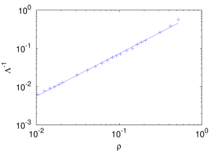
Figure 9: Parameter $\Lambda$ from the exponential fits in Fig. 4 as function of prey density.

Appendix B Exponents of Fig. 2, Fig. 4 and Fig. 6

We here present plots depicting the dependence of the parameter $\Lambda$ from Fig. 4 versus the prey density (Fig. 9) as well as of the scaling exponents $\beta$ and $\nu$ from Figs. 2 and 6.

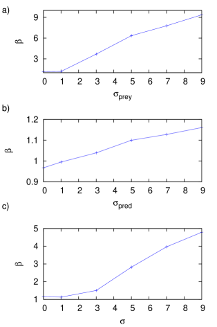
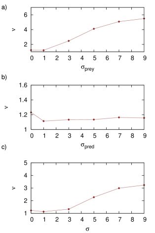
Figure 10: Left: Exponents of the power-law fits in Fig. 2 a) as function of the preys’ sighting range in case of a blind predator, b) as function of the predator’s sighting range in case of blind prey, c) as function of the sighting range in case of identical sighting ranges . Right: Exponents of the power-law fits in Fig. 6 a) as function of the preys’ sighting range in case of a blind predator, b) as function of the predator’s sighting range in case of blind prey, c) as function of the sighting range in case of identical sighting ranges . The lines are meant to guide the eye.

References

References

- [1] Y. Chen, T. Kolokolnikov. 2014 A minimal model of predator-swarm interactions. J. R. Soc. Interface 11 20131208.
- [2] R. S. Olson, A. Hintze, F. C. Dyer, D. B. Knoester, C. Adami. 2013 Predator confusion is sufficient to evolve swarming behaviour. J. R. Soc. Interface 10 20130305.
- [3] S. Redner, K. Kang. 1984 Kinetics of the ’scavenger’ reaction. J. Phys. A 17 L451.
- [4] A. Blumen, G. Zumofen, J. Klafter. 1984 Target annihilation by random walkers. Phys. Rev. B 30 5379(R).
- [5] A. J. Bray, R. A. Blythe. 2002 Exact asymptotics for one-dimensional diffusion with mobile traps. Phys. Rev. Lett. 89 150601.
- [6] G. Oshanin, O. Bénichou, M. Coppey, M. Moreau. 2002 Trapping reactions with randomly moving traps: exact asymptotic results for compact exploration. Phys. Rev. E 66 060101(R).
- [7] M. Moreau, G. Oshanin, O. Bénichou, M. Coppey. 2004 Lattice theory of trapping reactions with mobile species. Phys. Rev. E 69 046101.
- [8] S. B. Yuste, G. Oshanin, K. Lindenberg, O. Bénichou, J. Klafter. 2008 Survival probability of a particle in a sea of mobile traps: A tale of tails. Phys. Rev. E 78 021105.
- [9] P. L. Krapivsky, S. Redner. 1996 Kinetics of a diffusive capture process: Lamb besieged by a pride of lions. J. Phys. A 29 5347???5357.
- [10] S. Redner, P. L. Krapivsky. 1999 Capture of a lamb: Diffusing predators seeking a diffusing prey. Am. J. Phys. 67 1277.
- [11] W. Feller. 1971 An Introduction to Probability Theory, Vol. 1. New York, USA: Wiley & Sons.
- [12] G. H. Weiss. 1994 Aspects and Applications of the Random Walk Amsterdam, Netherlands: North Holland.
- [13] D. Campos, E. Abad, V. Mendez, S. B. Yuste, K. Lindenberg. 2015 Optimal search strategies of space-time coupled random walkers with finite lifetimes. Phys. Rev. E 91 052115.
- [14] J. Wang, W. Li. 2015 Motion patterns and phase-transition of a i defender-intruder problem and optimal interception strategy of the defender. Commun. Nonlinear Sci. Numer. Simul. 27 294.
- [15] M. Sato. 2012 Chasing and escaping by three groups of species. Phys. Rev. E 85 066102.
- [16] A. Gabel, S. N. Majumdar, N. K. Panduranga, S. Redner. 2012 Can a lamb reach a haven before being eaten by diffusiong lions? J. Stat. Mech. P05011.
- [17] G. Oshanin, O. Vasilyev, P. L. Krapivsky, J. Klafter. 2009 Survival of an evasive prey. Proc. Natl Acad. Sci. USA 106 13696.
- [18] A. Sengupta, T. Kruppa, H. Loewen. 2011 Chemotactic predator-prey dynamics. Phys. Rev. E 81 031914.
- [19] R. Martínez-García,J. M. Calabrese, T. Mueller, K. Olson, C. López. 2013 Optimizing the search for resources by sharing information: Mongolian gazelles as a case study. Phys. Rev. Lett. 110 248106.
- [20] M. Bruna, S. J. Chapman. 2012 Diffusion of multiple species with excluded-volume effects. J. Chem. Phys. 137 204116.
- [21] M. Bruna, S. J. Chapman. 2012 Excluded-volume effects in the diffusion of hard spheres. Phys. Rev. E 85 011103.
- [22] S. Yang, S. Jiang, L. Jiang, G. Li, Z. Han. 2014 Aggregation increases prey survival time in group chase and escape. New J. Phys. 16 083006.
- [23] M. J. Seitz, G. Köster. 2014 How update schemes influence crowd simulations. J. Stat. Mech. P07002.
- [24] G. N. Watson. 1922 A Treatise on the Theory of Bessel Functions Cambridge, UK: Cambridge University Press.
- [25] G. E. Ornstein, L. S. Uhlenbeck. 1930 On the Theory of the Brownian Motion. Phys. Rev. 36 823.
- [26] S. Redner. 2001 A Guide to First-Passage Processes. Cambridge, UK: Cambridge University Press.
- [27] N. G. Van Kampen. 2007 Stochastic Processes in Physics and Chemistry, 3rd edn. Amsterdam, Netherlands: North Holland 1981.
- [28] A. Kamimura, T. Ohira. 2010 Group chase and escape. New J. Phys. 12 053013.
- [29] T. Iwama, M. Sato. 2012 Group chase and escape with some fast chasers. Phys. Rev. E 86 067102.
- [30] L. Angelani. 2012 Collective Predation and Escape Strategies. Phys. Rev. Lett. 109 118104.
- [31] R. Nishi, A. Kamimura, K. Nishinari T. Ohira. 2012 Group chase and escape with conversion from targets to chasers. Physica A 391 337.
- [32] A. Ramanantoanina, C. Hui, A. Ouhinou. 2011 Effects of density-dependent dispersal behaviours on the speed and spatial patterns of range expansion in predator-prey metapopulations. Ecol. Model. 222 3524.
- [33] T. Vicsek. 2010 Statistical Physics: Closing in on evaders. Nature 466 43.
- [34] V. V. Palyulin, A. V. Chechkin, R. Metzler. 2014 Lévy flights do not always optimize random blind search for sparse targets Proc. Natl Acad. Sci. USA 111 (8) 2931.
- [35] F. Bartumeus, M. G E. da Luz, G. M. Viswanathan, J. Catalan. 2005 Animal search strategies: a quantitative random-walk analysis. Ecology 86 3078.
- [36] L. C. M. Salvador, F. Bartumeus, S. A. Levin, W. S. Ryu. 2014 Mechanistic analysis of the search behaviour of Caenorhabditis elegans. J. R. Soc. Interface 11 20131092.
- [37] O. Bénichou, C. Loverdo, M. Moreau, R. Voituriez. 2006 Bidimensional intermittent search processes: an alternative to Lévy flights strategies. Phys. Rev. E 74 020102(R).
- [38] O. Bénichou, C. Loverdo, M. Moreau, and R. Voituriez. 2011 Intermittent search strategies. Rev. Mod. Phys. 83 81.
- [39] M. A. Lomholt, T. Koren, R. Metzler, J. Klafter. 2008 Lévy strategies in intermittent search processes are advantageous. Proc. Natl. Acad. Sci. USA 105 (32) 11055.
- [40] G. M. Viswanathan, S. V. Buldyrev, S. Havlin, M. G. E. da Luz, E. P. Raposo, H. Eugene Stanley. 1999 Optimizing the success of random searches Nature 401 911.
- [41] G. M. Viswanathan, V. Afanasyev, S. V. Buldyrev, E. J. Murphy, P. A. Prince, H. E. Stanley. 1996 Lévy flight search patterns of wandering albatrosses Nature 381 413.
- [42] N. E. Humphries, H. Weimerskirch, N. Queiroz, E. J. Southall, D. W. Sims. 2012 Foraging success of biological Lévy flights recorded in situ Proc. Natl. Acad. Sci. USA 109 7169.
- [43] D. W. Sims et al.. 2008 Scaling laws of marine predator search behaviour. Nature 451 1098.
- [44] D. W. Sims et al.. 2010 Environmental context explains Lévy and Brownian movement patterns of marine predators Nature 465 1066.
- [45] M. Moreau, G. Oshanin, M. Coppey, O. Bénichou. 2003 Pascal Principle for Diffusion-Controlled Trapping Reactions. Phys. Rev. E 67 045104.
- [46] R. A. Blythe and A. J. Bray. 2003 Survival probability of a diffusing particle in the presence of Poisson-distributed mobile traps. Phys. Rev. E 67 041101.
- [47] A. J. Bray, S. N. Majumdar, R. A. Blythe. 2003 Formal solution of a class of reaction-diffusion models: Reduction to a single-particle problem. Phys. Rev. E 67 060102.
- [48] B. Meerson, A. Vilenkin, P. L. Krapivsky. 2014 Survival of a static target in a gas of diffusing particles with exclusion. Phys. Rev. E 90 022120.
- [49] L. Bertini, A. De Sole, D. Gabrielli, G. Jona-Lasinio, C. Landim. 2015 Macroscopic fluctuation theory. Rev. Mod. Phys. 87 593.