Separating Overlapped Intervals on a Line

Abstract

Given $n$ intervals on a line $\ell$, we consider the problem of moving these intervals on $\ell$ such that after the movement no two intervals overlap and the maximum moving distance of the intervals is minimized. The difficulty for solving the problem lies in determining the order of the intervals in an optimal solution. By interesting observations, we show that it is sufficient to consider at most $n$ “candidate” lists of ordered intervals. Further, although explicitly maintaining these lists takes $\Omega(n^{2})$ time and space, by more observations and a pruning technique, we present an algorithm that can compute an optimal solution in $O(n\log n)$ time and $O(n)$ space. We also prove an $\Omega(n\log n)$ time lower bound for solving the problem, which implies the optimality of our algorithm.

1 Introduction

Let $\mathcal{I}$ be a set of $n$ intervals on a real line $\ell$. We say that two intervals overlap if their intersection contains more than one point. In this paper, we consider an interval separation problem: move the intervals of $\mathcal{I}$ on $\ell$ such that no two intervals overlap and the maximum moving distance of these intervals is minimized.

If all intervals of $\mathcal{I}$ have the same length, then after the left endpoints of the intervals are sorted, the problem can be solved in $O(n)$ time by an easy greedy algorithm [15]. For the general problem where intervals may have different lengths, to the best of our knowledge, the problem has not been studied before. In this paper, we present an $O(n\log n)$ time and $O(n)$ space algorithm for it. We also show an $\Omega(n\log n)$ time lower bound for solving the problem under the algebraic decision tree model, and thus our algorithm is optimal.

As a basic problem and like many other interval problems, the interval separation problem potentially has many applications. For example, one possible application is on scheduling, as follows. Suppose there are $n$ jobs that need to be completed on a machine. Each job requests a starting time and a total time for using the machine (hence it is a time interval). The machine can only work on one job at any time, and once it works on one job, it is not allowed to switch to other jobs until the job is finished. If the requested time intervals of the jobs have any overlap, then we have to change the requested starting times of some intervals. In order to minimize deviations from their requested time intervals, one scheduling strategy could be changing the requested starting times (either advance or delay) such that the maximum difference between the requested starting times and the scheduled starting times of all jobs is minimized. Clearly, the problem is an instance of the interval separation problem. The problem also has applications in the following scenario. Suppose a wireless sensor network has $n$ wireless mobile devices on a line and each device has a transmission range. We want to move the devices along the line to eliminate the interference such that the maximum moving distance of the devices is minimized (e.g., to save the energy). This is also an instance of the interval separation problem.

1.1 Related Work

Many interval problems have been used to model scheduling problems. We give a few examples. Given $n$ jobs, each job requests a time interval to use a machine. Suppose there is only one machine and the goal is to find a maximum number of jobs whose requested time intervals do not have any overlap (so that they can use the machine). The problem can be solved in $O(n\log n)$ time by an easy greedy algorithm [11]. Another related problem is to find a minimum number of machines such that all jobs can be completed [11]. Garey et al. [10] studied a scheduling problem, which is essentially the following problem. Given $n$ intervals on a line, determine whether it is possible to find a unit-length sub-interval in each input interval, such that no two sub-intervals overlap. An $O(n\log n)$ time algorithm was given in [10] for it. An optimization version of the problem was also studied [7, 20], where the goal is to find a maximum number of intervals that contain non-overlapping unit-length sub-intervals. Other scheduling problems on intervals have also been considered, e.g., see [6, 10, 11, 12, 13, 19, 21].

Many problems on wireless sensor networks are also modeled as interval problems. For example, a mobile sensor barrier coverage problem can be modeled as the following interval problem. Given on a line $n$ intervals (each interval is the region covered by a sensor at the center of the interval) and another segment $B$ (called “barrier”), the goal is to move the intervals such that the union of the intervals fully covers $B$ and the maximum moving distance of all intervals is minimized. If all intervals have the same length, Czyzowicz et al. [8] solved the problem in $O(n^{2})$ time and later Chen et al. [4] improved it to $O(n\log n)$ time. If intervals have different lengths, Chen et al. [4] solved the problem in $O(n^{2}\log n)$ time. The min-sum version of the problem has also been considered. If intervals have the same length, Czyzowicz et al. [9] gave an $O(n^{2})$ time algorithm, and Andrews and Wang [1] solved the problem in $O(n\log n)$ time. If intervals have different lengths, then the problem becomes NP-hard [4]. Refer to [2, 3, 5, 14, 17, 18] for other interval problems on mobile sensor barrier coverage.

Our interval separation problem may also be considered as a coverage problem in the sense that we want to move intervals of $\mathcal{I}$ to cover a total of maximum length of the line $\ell$ such that the maximum moving distance of the intervals is minimized.

1.2 Our Approach

We consider a one-direction version of the problem in which intervals of $\mathcal{I}$ are only allowed to move rightwards. We show (in Section 2) that the original “two-direction” problem can be reduced to the one-direction problem in the following way: If OPT is an optimal solution of the one-direction problem and $\delta_{opt}$ is the maximum moving distance of all intervals in OPT, then we can obtain an optimal solution for the two-direction problem by moving each interval in OPT leftwards by $\delta_{opt}/2$.

Hence, it is sufficient to solve the one-direction problem. It turns out that the difficulty is mainly on determining the order of intervals of $\mathcal{I}$ in OPT. Indeed, once such an “optimal order” is known, it is quite straightforward to compute the positions of the intervals in OPT in additional $O(n)$ time (i.e., consider the intervals in the order one by one and put each interval “as left as possible”). If all intervals have the same length, then such an optimal order is obvious, which is the order of the intervals sorted by their left endpoints in the input. Indeed, this is how the $O(n)$ time algorithm in [15] works.

However, if the intervals have different lengths, which is the case we consider in this paper, then determining an optimal order is substantially more challenging. At first glance, it seems that we have to consider all possible orders of the intervals, whose number is exponential. By several interesting (and even surprising) observations, we show that we only need to consider at most $n$ ordered lists of intervals. Consequently, a straightforward algorithm can find and maintain these “candidate” lists in $O(n^{2})$ time and space. We call it the “preliminary algorithm”, which is essentially a greedy algorithm. The algorithm is relatively simple but it is quite involved to prove its correctness. To this end, we extensively use the “exchange argument”, which is a standard technique for proving correctness of greedy algorithms (e.g., see [11]).

To further improve the preliminary algorithm, we discover more observations, which help us “prune” some “redundant” candidate lists. More importantly, the remaining lists have certain monotonicity properties such that we are able to implicitly compute and maintain them in $O(n\log n)$ time and $O(n)$ space, although the number of the lists can still be $\Omega(n)$. Although the correctness analysis is fairly complicated, the algorithm is still quite simple and easy to implement (indeed, the most “complicated” data structure is a binary search tree).

The rest of the paper is organized as follows. In Section 2, we give notation and reduce our problem to the one-direction case. In Section 3, we give our preliminary algorithm, whose correctness is proved in Section 4. The improved algorithm is presented in Section 5. In Section 6, we conclude the paper and prove the $\Omega(n\log n)$ time lower bound by a reduction from the integer element distinctness problem [16, 22].

2 Preliminaries

We assume the line $\ell$ is the $x$-axis. The one-direction version of the interval separation problem is to move intervals of $\mathcal{I}$ on $\ell$ in one direction (without loss of generality, we assume it is the right direction) such that no two intervals overlap and the maximum moving distance of the intervals is minimized. Let OPT denote an optimal solution of the one-direction version and let $\delta_{opt}$ be the maximum moving distance of all intervals in OPT. The following lemma gives a reduction from the general “two-direction” problem to the one-direction problem.

Lemma 1

An optimal solution for the interval separation problem can be obtained by moving every interval in OPT leftwards by $\delta_{opt}/2$.

Proof

Let $SOL$ be the solution obtained by moving every interval in OPT leftwards by $\delta_{opt}/2$. Our goal is to show that $SOL$ is an optimal solution for our original problem. Let $\delta$ be the maximum moving distance of all intervals in $SOL$. Since no intervals in OPT have been moved leftwards (with respect to their input positions), we have $\delta=\delta_{opt}/2$.

Assume to the contrary that $SOL$ is not optimal. Then, there exists another solution $SOL^{\prime}$ for the original problem in which the maximum interval moving distance is $\delta^{\prime}<\delta$. By moving every interval of $SOL^{\prime}$ rightwards by $\delta^{\prime}$, we can obtain a feasible solution $SOL^{\prime\prime}$ for the one-direction problem in which no interval has been moved leftwards (with respect to their input positions) and the maximum interval moving distance of $SOL^{\prime\prime}$ is at most $2\delta^{\prime}$, which is smaller than $\delta_{opt}$ since $\delta^{\prime}<\delta$. However, this contradicts with that OPT is an optimal solution for the one-direction case. ∎

By Lemma 1, once we have an optimal solution for the one-direction problem, we can obtain an optimal solution for our original problem in additional $O(n)$ time. In the following, we will focus on solving the one-direction case.

We first sort all intervals of $\mathcal{I}$ by their left endpoints. For ease of exposition, we assume no two intervals have their left endpoints located at the same position (otherwise we could break ties by also sorting their right endpoints). Let $\mathcal{I}=\{I_{1},I_{2},\ldots,I_{n}\}$ be the sorted intervals by their left endpoints from left to right. For each (integer) $i\in[1,n]$, denote by $l_{i}$ and $r_{i}$ the (physical) left and right endpoints of $I_{i}$, respectively. Denote by $x_{i}^{l}$ and $x_{i}^{r}$ the $x$-coordinates of $l_{i}$ and $r_{i}$ in the input, respectively. Note that for each $i\in[1,n]$, the two physical endpoints $l_{i}$ and $r_{i}$ may be moved during the algorithm, but the two coordinates $x_{i}^{l}$ and $x_{i}^{r}$ are always fixed. Denote by $|I_{i}|$ the length of $I_{i}$, i.e., $|I_{i}|=x_{i}^{r}-x_{i}^{l}$.

For convenience, when we say the position of an interval, we refer to the position of the left endpoint of the interval.

With respect to a subset $\mathcal{I}^{\prime}$ of $\mathcal{I}$, by a configuration of $\mathcal{I}^{\prime}$, we refer to a specification of the position of each interval of $\mathcal{I}^{\prime}$. For example, in the input configuration of $\mathcal{I}$, interval $I_{i}$ is at $x_{i}^{l}$ for each $i\in[1,n]$. Given a configuration $\mathcal{C}$ of $\mathcal{I}^{\prime}$, for each interval $I_{i}\in\mathcal{I}^{\prime}$, if $l_{i}$ is at $x$ in $\mathcal{C}$, then we call the value $x-x_{i}^{l}$ the displacement of $I_{i}$, denoted by $d(i,\mathcal{C})$, and if $d(i,\mathcal{C})\geq 0$, then we say that $I_{i}$ is valid in $\mathcal{C}$. We say that $\mathcal{C}$ is feasible if the displacement of every interval of $\mathcal{I}^{\prime}$ is valid and no two intervals of $\mathcal{I}^{\prime}$ overlap in $\mathcal{C}$. The maximum displacement of the intervals of $\mathcal{I}^{\prime}$ in $\mathcal{C}$ is called the max-displacement of $\mathcal{C}$, denoted by $\delta(\mathcal{C})$. Hence, finding an optimal solution for the one-direction problem is equivalent to computing a feasible configuration of $\mathcal{I}$ whose max-displacement is minimized; such a configuration is also called an optimal configuration.

For convenience of discussion, depending on the context, we will use the intervals $I_{i}$ of $\mathcal{I}$ and their indices $i$ interchangeably. For example, $\mathcal{I}$ may also refer to the set of indices $\{1,2,\ldots,n\}$.

Let $L_{opt}$ be the list of intervals of $\mathcal{I}$ in an optimal configuration sorted from left to right. We call $L_{opt}$ an optimal list. Given $L_{opt}$, we can compute an optimal configuration in $O(n)$ time by an easy greedy algorithm, called the left-possible placement strategy: Consider the intervals following their order in $L_{opt}$, and for each interval, place it on $\ell$ as left as possible so that it does not overlap with the intervals that are already placed on $\ell$ and its displacement is non-negative. The following lemma formally gives the algorithm and proves its correctness.

Lemma 2

Given an optimal list $L_{opt}$, we can compute an optimal configuration in $O(n)$ time by the left-possible placement strategy.

Proof

We first describe the algorithm and then prove its correctness.

We consider the indices one by one following their order in $L_{opt}$. Consider any index $i$. If $I_{i}$ is the first interval of $L_{opt}$, then we place $I_{i}$ at $x_{i}^{l}$ (i.e., $I_{i}$ stays at its input position). Otherwise, let $I_{j}$ be the previous interval of $I_{i}$ in $L_{opt}$. So $I_{j}$ has already been placed on $\ell$. Let $x$ be the current $x$-coordinate of the right endpoint $r_{j}$ of $I_{j}$. We place the left endpoint $l_{i}$ of $I_{i}$ at $\max\{x_{i}^{l},x\}$. If $I_{i}$ is the last interval of $L_{opt}$, then we finish the algorithm. Clearly, the algorithm can be easily implemented in $O(n)$ time.

Let $\mathcal{C}$ be the configuration of all intervals obtained by the above algorithm. Recall that $\delta(\mathcal{C})$ denote the max-displacement of $\mathcal{C}$. Below, we show that $\mathcal{C}$ is an optimal configuration.

Indeed, since $L_{opt}$ is an optimal list, there exists an optimal configuration $\mathcal{C}^{\prime}$ in which the order of the indices of $\mathcal{I}$ follows that in $L_{opt}$. Hence, the max-displacement of $\mathcal{C}^{\prime}$ is $\delta_{opt}$. According to our greedy strategy for computing $\mathcal{C}$, it is not difficult to see that the position of each interval $I_{i}$ of $\mathcal{I}$ in $\mathcal{C}$ cannot be strictly to the right of its position in $\mathcal{C}^{\prime}$. Therefore, the displacement of each interval in $\mathcal{C}$ is no larger than that in $\mathcal{C}^{\prime}$. This implies that $\delta(\mathcal{C})\leq\delta_{opt}$. Therefore, $\mathcal{C}$ is an optimal configuration. ∎

Due to Lemma 2, we will focus on computing an optimal list $L_{opt}$.

For any subset $\mathcal{I}^{\prime}$ of $\mathcal{I}$, an (ordered) list of $\mathcal{I}^{\prime}$ refers to a permutation of the indices of $\mathcal{I}^{\prime}$. Let $L$ be a list of $\mathcal{I}$ and let $L^{\prime}$ be a list of $\mathcal{I}^{\prime}$ with $\mathcal{I}^{\prime}\subseteq\mathcal{I}$. We say that $L^{\prime}$ is consistent with $L$ if the relative order of indices of $\mathcal{I}^{\prime}$ in $L$ is the same as that in $L^{\prime}$. If $L^{\prime}$ is consistent with an optimal list $L_{opt}$ of $\mathcal{I}$, then we call $L^{\prime}$ a canonical list of $\mathcal{I}^{\prime}$.

For any $1\leq i\leq j\leq n$, we use $\mathcal{I}[i,j]$ to denote the subset of consecutive intervals of $\mathcal{I}$ from $i$ to $j$, i.e, $\{i,i+1,\ldots,j\}$.

3 The Preliminary Algorithm

In this section, we describe an algorithm that can compute an optimal list in $O(n^{2})$ time and space. The correctness of the algorithm is mainly discussed in Section 4.

Our algorithm considers the intervals of $\mathcal{I}$ one by one by their index order. After each interval $I_{i}$ is processed, we obtain a set $\mathcal{L}$ of at most $i$ lists of the indices of $\mathcal{I}[1,i]$, such that $\mathcal{L}$ contains at least one canonical list of $\mathcal{I}[1,i]$. For each list $L\in\mathcal{L}$, a feasible configuration $\mathcal{C}_{L}$ of the intervals of $\mathcal{I}[1,i]$ is also maintained. As will be clear later, $\mathcal{C}_{L}$ is essentially the configuration obtained by applying the left-possible placement strategy on the intervals of $\mathcal{I}[1,i]$ following their order in $L$. For each $j\in[1,i]$, we let $x_{j}^{l}(\mathcal{C}_{L})$ and $x_{j}^{r}(\mathcal{C}_{L})$ respectively denote the $x$-coordinates of $l_{j}$ and $r_{j}$ in $\mathcal{C}_{L}$ (recall that $l_{j}$ and $r_{j}$ are the left and right endpoints of the interval $I_{j}$, respectively). Recall that $\delta(\mathcal{C}_{L})$ denotes the max-displacement of $\mathcal{C}_{L}$, i.e, the maximum displacement of the intervals of $\mathcal{I}[1,i]$ in $\mathcal{C}_{L}$.

Initially when $i=1$, we have only one list $L=\{1\}$ and let $\mathcal{C}_{L}$ consist of the single interval $I_{1}$ at its input position, i.e., $x_{1}^{l}(\mathcal{C}_{L})=x_{1}^{l}$. Clearly, $\delta(\mathcal{C}_{L})=0$. We let $\mathcal{L}$ consist of the only list $L$. It is vacuously true that $L$ is a canonical list of $\mathcal{I}[1,1]$.

In general, assume interval $I_{i-1}$ has been processed and we have the list set $\mathcal{L}$ as discussed above. In the following, we give our algorithm for processing $I_{i}$. Consider a list $L\in\mathcal{L}$. Note that $\mathcal{C}_{L}$ has been computed, which is a feasible configuration of $\mathcal{I}[1,i-1]$. The value $\delta(\mathcal{C}_{L})$ is also maintained. Let $m$ be the last index in $L$. Note that $m<i$. Depending on the values of $x_{i}^{l}$, $x_{i}^{r}$, $x_{m}^{r}$, and $x_{m}^{l}(\mathcal{C}_{L})$, there are three main cases (e.g. see Fig. 1).

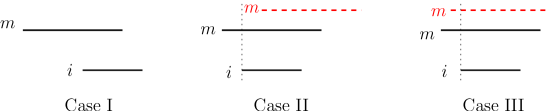
Figure 1: Illustrating the three main cases. The (black) solid segments show intervals in their input positions and the (red) dashed segments shows interval $I_{m}$ in $\mathcal{C}_{L}$.

Case I: $x_{i}^{r}\geq x_{m}^{r}$ (i.e., the right endpoint $r_{i}$ of $I_{i}$ is to the right of $r_{m}$ in the input).

In this case, we update $L$ by appending $i$ to the end of $L$. Further, we update the configuration $\mathcal{C}_{L}$ by placing $l_{i}$ at $\max\{x_{m}^{r}(\mathcal{C}_{L}),x_{i}^{l}\}$ (which follows the left-possible placement strategy). We let $L^{\prime}$ denote the original list of $L$ before $i$ is inserted and let $\mathcal{C}_{L^{\prime}}$ denote the original configuration of $\mathcal{C}_{L}$. We update $\delta(\mathcal{C}_{L})$ by the following observation.

Observation 1

$\mathcal{C}_{L}$ is a feasible configuration and $\delta(\mathcal{C}_{L})=\max\{\delta(\mathcal{C}_{L^{\prime}}),x_{i}^{l}(\mathcal{C}_{L})-x_{i}^{l}\}$.

Proof

By our way of setting $I_{i}$ in $\mathcal{C}_{L}$, $I_{i}$ is valid and does not overlap with any other interval in $\mathcal{C}_{L}$. Hence, $\mathcal{C}_{L}$ is feasible. Comparing with $\mathcal{C}_{L^{\prime}}$, $\mathcal{C}_{L}$ has one more interval $I_{i}$. Therefore, $\delta(\mathcal{C}_{L})$ is equal to the larger value of $\delta(\mathcal{C}_{L^{\prime}})$ and the displacement of $I_{i}$ in $\mathcal{C}_{L}$, which is $x_{i}^{l}(\mathcal{C}_{L})-x_{i}^{l}$. ∎

The following lemma will be used to show the correctness of our algorithm and its proof is deferred to Section 4.

Lemma 3

If $L^{\prime}$ is a canonical list of $\mathcal{I}[1,i-1]$, then $L$ is a canonical list of $\mathcal{I}[1,i]$.

Case II: $x_{i}^{r}<x_{m}^{r}$ and $x_{i}^{l}\leq x_{m}^{l}(\mathcal{C}_{L})$.

In this case, we update $L$ by inserting $i$ right before $m$. Let $x=x_{m}^{l}(\mathcal{C}_{L})$. We update $\mathcal{C}_{L}$ by setting $l_{i}$ at $x$ and setting $l_{m}$ at $x+|I_{i}|$. We let $L^{\prime}$ denote the original list of $L$ before inserting $i$ and let $\mathcal{C}_{L^{\prime}}$ denote the original $\mathcal{C}_{L}$. We update $\delta(\mathcal{C}_{L})$ by the following observation. Note that $x_{m}^{l}(\mathcal{C}_{L})$ now refers to the position of $l_{m}$ in the updated $\mathcal{C}_{L}$.

Observation 2

$\mathcal{C}_{L}$ is a feasible configuration and $\delta(\mathcal{C}_{L})=\max\{\delta(\mathcal{C}_{L^{\prime}}),x_{m}^{l}(\mathcal{C}_{L})-x_{m}^{l}\}$.

Proof

Since $x_{i}^{l}\leq x$ and $l_{i}$ is at $x$ in $\mathcal{C}_{L}$, $I_{i}$ is valid in $\mathcal{C}_{L}$. Comparing with its position in $\mathcal{C}_{L^{\prime}}$, $I_{m}$ has been moved rightwards; since $I_{m}$ is valid in $\mathcal{C}_{L^{\prime}}$, $I_{m}$ is also valid in $\mathcal{C}_{L}$. Note that no two intervals overlap in $\mathcal{C}_{L}$. Therefore, $\mathcal{C}_{L}$ is a feasible configuration.

Comparing with $\mathcal{C}_{L^{\prime}}$, $\mathcal{C}_{L}$ has one more interval $I_{i}$ and $I_{m}$ has been moved rightwards in $\mathcal{C}_{L}$. Therefore, $\delta(\mathcal{C}_{L})$ is equal to the maximum of the following three values: $\delta(\mathcal{C}_{L^{\prime}})$, the displacement of $I_{i}$ in $\mathcal{C}_{L}$, and the displacement of $I_{m}$ in $\mathcal{C}_{L}$. Observe that the displacement of $I_{i}$ is smaller than that of $I_{m}$. This is because $l_{m}$ is to the left of $l_{i}$ in the input (since $m<i$) while $l_{m}$ is to the right of $l_{i}$ in $\mathcal{C}_{L}$. Thus, it holds that $\delta(\mathcal{C}_{L})=\max\{\delta(\mathcal{C}_{L^{\prime}}),x_{m}^{l}(\mathcal{C}_{L})-x_{m}^{l}\}$. ∎

The proof of the following lemma is deferred to Section 4.

Lemma 4

If $L^{\prime}$ is a canonical list of $\mathcal{I}[1,i-1]$, then $L$ is a canonical list of $\mathcal{I}[1,i]$.

Case III: $x_{i}^{r}<x_{m}^{r}$ and $x_{i}^{l}>x_{m}^{l}(\mathcal{C}_{L})$.

In this case, we first update $L$ by appending $i$ to the end of $L$ and update $\mathcal{C}_{L}$ by placing the left endpoint of $I_{i}$ at $x_{m}^{r}(\mathcal{C}_{L})$. Let $L^{\prime}$ be the original list $L$ before we insert $i$ and let $\mathcal{C}_{L^{\prime}}$ be the original configuration of $\mathcal{C}_{L}$.

Further, we create a new list $L^{*}$, which is the same as $L$ except that we switch the order of $i$ and $m$. Thus, $m$ is the last index of $L^{*}$. Correspondingly, the configuration $\mathcal{C}_{L^{*}}$ is the same as $\mathcal{C}_{L}$ except that $l_{i}$ is at $x_{i}^{l}$, i.e., its position in the input, and $l_{m}$ is at $x_{i}^{r}$. We say that $L^{*}$ is the new list generated by $L^{\prime}$. We do not put $L^{*}$ in the set $\mathcal{L}$ at this moment (but $L$ is in $\mathcal{L}$).

Observation 3

Both $\mathcal{C}_{L}$ and $\mathcal{C}_{L^{*}}$ are feasible; $\delta(\mathcal{C}_{L})=\max\{\delta(\mathcal{C}_{L^{\prime}}),x_{i}^{l}(\mathcal{C}_{L})-x_{i}^{l}\}$ and $\delta(\mathcal{C}_{L^{*}})=\max\{\delta(\mathcal{C}_{L^{\prime}}),x_{m}^{l}(\mathcal{C}_{L^{*}})-x_{m}^{l}\}$.

Proof

By a similar argument as in Observation 1, $\mathcal{C}_{L}$ is feasible and $\delta(\mathcal{C}_{L})=\max\{\delta(\mathcal{C}_{L^{\prime}}),x_{i}^{l}(\mathcal{C}_{L})-x_{i}^{l}\}$. By a similar argument as in Observation 2, $\mathcal{C}_{L^{*}}$ is feasible and $\delta(\mathcal{C}_{L^{*}})=\max\{\delta(\mathcal{C}_{L^{\prime}}),x_{m}^{l}(\mathcal{C}_{L^{*}})-x_{m}^{l}\}$. We omit the details. ∎

The proof of the following lemma is deferred to Section 4.

Lemma 5

If $L^{\prime}$ is a canonical list of $\mathcal{I}[1,i-1]$, then one of $L$ and $L^{*}$ is a canonical list of $\mathcal{I}[1,i]$.

After each list $L$ of $\mathcal{L}$ is processed as above, let $\mathcal{L}^{*}$ denote the set of all new generated lists in Case III. Recall that no list of $\mathcal{L}^{*}$ has been added into $\mathcal{L}$ yet. Let $L^{*}_{min}$ be the list of $\mathcal{L}^{*}$ with the minimum value $\delta(\mathcal{C}_{L^{*}_{min}})$. The proof of the following lemma is deferred to Section 4.

Lemma 6

If $\mathcal{L}^{*}$ has a canonical list of $\mathcal{I}[1,i]$, then $L^{*}_{min}$ is a canonical list of $\mathcal{I}[1,i]$.

Due to Lemma 6, among all lists of $\mathcal{L}^{*}$, we only need to keep $L_{min}^{*}$. So we add $L^{*}_{min}$ to $\mathcal{L}$ and ignore all other lists of $\mathcal{L}^{*}$. We call $L^{*}_{min}$ a new list of $\mathcal{L}$ produced by our algorithm for processing $I_{i}$ and all other lists of $\mathcal{L}$ are considered as the old lists.

Remark.

Lemma 6 is a key observation that helps avoid maintaining an exponential number of lists.

This finishes our algorithm for processing the interval $I_{i}$. Clearly, $\mathcal{L}$ has at most one more new list. After $I_{n}$ is processed, the list $L$ of $\mathcal{L}$ with minimum $\delta(\mathcal{C}_{L})$ is an optimal list.

According to our above description, the algorithm can be easily implemented in $O(n^{2})$ time and space. The proof of Theorem 3.1 gives the details and also shows the correctness of the algorithm based on Lemmas 3, 4, 5, and 6.

Theorem 3.1

An optimal solution for the one-direction problem can be found in $O(n^{2})$ time and space.

Proof

To implement the algorithm, we can use a linked list to represent each list of $\mathcal{L}$. Consider a general step for processing interval $I_{i}$.

For any list $L\in\mathcal{L}$, inserting $i$ to $L$ can be easily done in $O(1)$ time for each of the three cases. The configuration $\mathcal{C}_{L}$ and the value $\delta(\mathcal{C}_{L})$ can also be updated in $O(1)$ time. If $L$ generates a new list $L^{*}$, then we do not explicitly construct $L^{*}$ but only compute the value $\delta(\mathcal{C}_{L^{*}})$, which can be done in $O(1)$ time by Observation 3. Once every list $L\in\mathcal{L}$ has been processed, we find the list $L^{*}_{min}\in\mathcal{L}^{*}$. Then, we explicitly construct $L^{*}$ and $\mathcal{C}_{L^{*}}$, in $O(n)$ time.

Hence, each general step for processing $I_{i}$ can be done in $O(n)$ time since $\mathcal{L}$ has at most $n$ lists. Thus, the total time and space of the algorithm is $O(n^{2})$.

For the correctness, after a general step for processing $I_{i}$, Lemmas 3, 4, 5, and 6 together guarantee that the set $\mathcal{L}$ has at least one canonical list of $\mathcal{I}[1,i]$. After $I_{n}$ is processed, since $\mathcal{C}_{L}$ is essentially obtained by the left-possible placement strategy for each list $L\in\mathcal{L}$, if $L$ is the list of $\mathcal{L}$ with the smallest $\delta(\mathcal{C}_{L})$, then $L$ is an optimal list and $\mathcal{C}_{L}$ is an optimal configuration by Lemma 2. ∎

4 The Correctness of the Preliminary Algorithm

In this section, we establish the correctness of our preliminary algorithm. Specifically, we will prove Lemmas 3, 4, 5, and 6. The major analysis technique is the exchange argument, which is quite standard for proving correctness of greedy algorithms (e.g., see [11]).

Let $L$ be a list of all indices of $\mathcal{I}$. For any two indices $j,k\in[1,n]$, let $L[j,k]$ denote the sub-list of all indices of $L$ between $j$ and $k$ (including $j$ and $k$).

For any $1\leq j<k\leq n$, we say that $(j,k)$ is an inversion of $L$ if $x_{j}^{r}\leq x_{k}^{r}$ and $k$ is before $j$ in $L$ ($k$ and $j$ are not necessarily consecutive in $L$; e.g., see Fig. 2 with $L=L_{opt}$). For an inversion $(j,k)$, we further introduce two sets of indices $L^{1}[j,k]$ and $L^{2}[j,k]$ as follows (e.g., see Fig. 2 with $L=L_{opt}$). Let $L^{1}[j,k]$ consist of all indices $i\in L[j,k]$ such that $i<k$ and $i\neq j$; let $L^{2}[j,k]$ consist of all indices $i\in L[j,k]$ such that $i\geq k$. Hence, $L^{1}[j,k]$, $L^{2}[j,k]$, and $\{j\}$ form a partition of the indices of $L[j,k]$.

Figure 2: Illustrating an inversion $(j,k)$ of $L_{opt}$ and an example for Lemma 7: the intervals $j$ and $k$ are shown in their input positions.

We first give the following lemma, which will be extensively used later.

Lemma 7

Let $L_{opt}$ be an optimal list of all indices of $\mathcal{I}$. If $L_{opt}$ has an inversion $(j,k)$, then there exists another optimal list $L_{opt}^{\prime}$ that is the same as $L_{opt}$ except that the sublist $L_{opt}[j,k]$ is changed to the following: all indices of $L_{opt}^{1}[j,k]$ are before $j$ and all indices of $L_{opt}^{2}[j,k]$ are after $j$ (in particular, $k$ is after $j$, so $(j,k)$ is not an inversion any more in $L^{\prime}_{opt}$), and further, the relative order of the indices of $L^{1}_{opt}[j,k]$ in $L^{\prime}_{opt}$ is the same as that in $L_{opt}$ (but this may not be the case for $L^{2}_{opt}[j,k]$). E.g., see Fig. 2.

Many proofs given later in the paper will utilize Lemma 7 as a basic technique for “eliminating” inversions in optimal lists. Before giving the proof of Lemma 7, which is somewhat technical, lengthy, and tedious, we first show that Lemma 3 can be easily proved with the help of Lemma 7.

4.1 Proof of Lemma 3.

Assume $L^{\prime}$ is a canonical list of $\mathcal{I}[1,i-1]$. Our goal is to prove that $L$ is a canonical list of $\mathcal{I}[1,i]$.

Since $L^{\prime}$ is a canonical list, by the definition of a canonical list, there exists an optimal configuration $\mathcal{C}$ in which the order of the intervals of $\mathcal{I}[1,i-1]$ is the same as that in $L^{\prime}$. Let $L_{opt}$ be the list of indices of the intervals of $\mathcal{I}$ in $\mathcal{C}$. If ${i}$ is after $m$ in $L_{opt}$, then $L$ is consistent with $L_{opt}$ and thus is a canonical list of $\mathcal{I}[1,i]$. In the following, we assume $i$ is before $m$ in $L_{opt}$.

Since $m<i$, $x_{m}^{r}\leq x_{i}^{r}$, and $i$ is before $m$ in $L_{opt}$, $(m,i)$ is an inversion in $L_{opt}$. Let $L^{\prime}_{opt}$ be another optimal list obtained by applying Lemma 7 on $(m,i)$. Refer to Fig. 3. We claim that $L$ is consistent with $L^{\prime}_{opt}$, which will prove that $L$ is a canonical list. We prove the claim below.

Figure 3: Illustrating the proof of Lemma 3. The intervals $m$ and $i$ are shown in their input positions.

Indeed, note that $L^{\prime}$ is consistent with $L_{opt}$. Comparing with $L_{opt}$, by Lemma 7, only the indices of the sublist $L_{opt}[m,i]$ have their relative order changed in $L_{opt}^{\prime}$. Since all indices of $L^{\prime}$ are smaller than $i$, by definition, all indices of $L^{\prime}$ that are in $L_{opt}[m,i]$ are contained in $L_{opt}^{1}[m,i]$. By Lemma 7, the relative order of the indices of $L_{opt}^{1}[m,i]$ in $L^{\prime}_{opt}$ is the same as that in $L_{opt}$, and further, all indices of $L_{opt}^{1}[m,i]$ are still before $m$ in $L^{\prime}_{opt}$. This implies that the relative order of the indices of $L^{\prime}$ does not change from $L_{opt}$ to $L^{\prime}_{opt}$. Hence, $L^{\prime}$ is consistent with $L^{\prime}_{opt}$. On the other hand, by Lemma 7, $i$ is after $m$. Thus, $L$ is consistent with $L^{\prime}_{opt}$. This proves the claim and thus proves Lemma 3.

4.2 Proof of Lemma 7

In this section, we give the proof of Lemma 7.

We partition the set $L_{opt}^{2}[j,k]\setminus\{k\}$ into two sets $S_{1}$ and $S_{2}$, defined as follows (e.g., see Fig. 4). Let $S_{1}$ consists of all indices $t$ of $L_{opt}^{2}[j,k]\setminus\{k\}$ such that $x_{t}^{r}\leq x_{j}^{r}$ (i.e., $r_{t}$ is to the left of $r_{j}$ in the input). Let $S_{2}$ consists of all indices of $L_{opt}^{2}[j,k]\setminus\{k\}$ that are not in $S_{1}$. Note that $L_{opt}[j,k]=L_{opt}^{1}[j,k]\cup S_{1}\cup S_{2}\cup\{j,k\}$. To simplify the notation, let $S=L_{opt}[j,k]$ and $S_{0}=L_{opt}^{1}[j,k]$ (e.g., see Fig. 4).

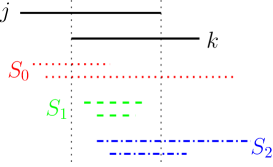
Figure 4: Illustrating the intervals of $L_{opt}[j,k]$ in their input positions. The two (red) dotted intervals are in $S_{0}=L_{opt}^{1}[j,k]$; the two (green) dashed intervals are in $S_{1}$; the two (blue) dashed-dotted intervals are in $S_{2}$.

We only consider the general case where none of $S_{0}$, $S_{1}$, and $S_{2}$ is empty since other cases can be analyzed by similar but simpler techniques.

In the following, from $L_{opt}$, we will subsequently construct a sequence of optimal lists $L_{0},L_{1},L_{2},L_{3}$, such that eventually $L_{3}$ is the list $L^{\prime}_{opt}$ specified in the statement of Lemma 7 (e.g., see Fig. 5).

4.2.1 The List $L_{0}$

For any adjacent indices $h$ and $g$ of $L_{opt}[j,k]\setminus\{j,k\}$ such that $h$ is before $g$ in $L_{opt}$, we say that $(h,g)$ is an exchangeable pair if one of the three cases happen: $g\in S_{0}$ and $h\in S_{1}$; $g\in S_{1}$ and $h\in S_{2}$; $g\in S_{0}$ and $h\in S_{2}$.

In the following, we will perform certain “exchange operations” to eliminate all exchangeable pairs of $L_{opt}$, after which we will obtain another optimal list $L_{0}$ in which for any $i_{0}\in S_{0}$, $i_{1}\in S_{1}$, $i_{2}\in S_{2}$, $i_{0}$ is before $i_{1}$ and $i_{2}$ is after $i_{1}$, and all other indices of $L_{0}$ have the same positions as in $L_{opt}$ (e.g., see Fig. 5).

Figure 5: Illustrating the relative order of $k,j,S_{0},S_{1},S_{2}$ in the four lists $L_{0},L_{1},L_{2}.L_{3}$.

Consider any exchangeable pair $(h,g)$ of $L_{opt}$. Let $L^{\prime}$ be another list that is the same as $L_{opt}$ except that $h$ and $g$ exchange their order. We call this an exchange operation. In the following, we show that $L^{\prime}$ is an optimal list.

Since $L_{opt}$ is an optimal list, there is an optimal configuration $\mathcal{C}$ in which the order of the intervals is the same as $L_{opt}$. Consider the configuration $\mathcal{C}^{\prime}$ that is the same as $\mathcal{C}$ except that we exchange the order of $h$ and $g$ in the following way (e.g., see Fig 6): $x_{g}^{l}(\mathcal{C}^{\prime})=x_{h}^{l}(\mathcal{C})$ and $x_{h}^{r}(\mathcal{C}^{\prime})=x_{g}^{r}(\mathcal{C})$, i.e., the left endpoint $l_{g}$ of $I_{g}$ in $\mathcal{C}^{\prime}$ is at the same position as $l_{h}$ in $\mathcal{C}$ and the right end point $r_{h}$ of $I_{h}$ in $\mathcal{C}^{\prime}$ is at the same position as $r_{g}$ in $\mathcal{C}$. Clearly, the order of intervals in $\mathcal{C}^{\prime}$ is the same as that in $L^{\prime}$. In the following, we show that $\mathcal{C}^{\prime}$ is an optimal configuration, which will prove that $L^{\prime}$ is an optimal list.

Figure 6: Left: Illustrating the intervals $g$ and $h$ at their input positions. Right: Illustrating the two intervals $h$ and $g$ in the configurations $\mathcal{C}$ and $\mathcal{C}^{\prime}$ (note that $h$ and $g$ do not have to be connected).

We first show that $\mathcal{C}^{\prime}$ is feasible. Recall that intervals $h$ and $g$ are adjacent in $L_{opt}$ and also in $L^{\prime}$. By our way of setting $I_{g}$ and $I_{h}$ in $\mathcal{C}^{\prime}$, The segments of $\ell$ “spanned” by $I_{h}$ and $I_{g}$ in both $\mathcal{C}$ and $\mathcal{C}^{\prime}$ are exactly the same (e.g., the segments between the two vertical dotted lines in Fig. 6). Since no two intervals of $\mathcal{I}$ overlap in $\mathcal{C}$, no two intervals overlap in $\mathcal{C}^{\prime}$ as well.

Next, we show that every interval of $\mathcal{I}$ is valid in $\mathcal{C}^{\prime}$. To this end, it is sufficient to show that $I_{h}$ and $I_{g}$ are valid in $\mathcal{C}^{\prime}$ since other intervals do not change positions from $\mathcal{C}$ to $\mathcal{C}^{\prime}$. For $I_{h}$, comparing with its position in $\mathcal{C}$, $I_{h}$ has been moved rightwards in $\mathcal{C}^{\prime}$, and thus $I_{h}$ is valid in $\mathcal{C}^{\prime}$. For $I_{g}$, since $(h,g)$ is an exchangeable pair, $g$ is either in $S_{0}$ or in $S_{1}$. In either case, $x_{g}^{l}\leq x_{k}^{r}$. On the other hand, $I_{k}$ is to the left of $I_{g}$ in $\mathcal{C}^{\prime}$, which implies that $x_{k}^{r}(\mathcal{C}^{\prime})\leq x_{g}^{l}(\mathcal{C}^{\prime})$. Since $I_{k}$ does not change position from $\mathcal{C}$ to $\mathcal{C}^{\prime}$ and $I_{k}$ is valid in $\mathcal{C}$, we have $x_{k}^{r}\leq x_{k}^{r}(\mathcal{C})=x_{k}^{r}(\mathcal{C}^{\prime})$. Combining the above discussion, we have $x_{g}^{l}\leq x_{k}^{r}\leq x_{k}^{r}(\mathcal{C})=x_{k}^{r}(\mathcal{C}^{\prime})\leq x_{g}^{l}(\mathcal{C}^{\prime})$. Thus, $I_{g}$ is valid in $\mathcal{C}^{\prime}$. This proves that $\mathcal{C}^{\prime}$ is a feasible configuration.

We proceed to show that $\mathcal{C}^{\prime}$ is an optimal configuration by proving that the max-displacement of $\mathcal{C}^{\prime}$ is no more than the max-displacement of $\mathcal{C}$, i.e., $\delta(\mathcal{C}^{\prime})\leq\delta(\mathcal{C})$. Note that $\delta(\mathcal{C})=\delta_{opt}$ since $\mathcal{C}$ is an optimal configuration. Comparing with $\mathcal{C}$, $I_{g}$ has been moved leftwards and $I_{h}$ has been moved rightwards in $\mathcal{C}^{\prime}$. Therefore, to prove $\delta(\mathcal{C}^{\prime})\leq\delta_{opt}$, it suffices to show that the displacement of $I_{h}$ in $\mathcal{C}^{\prime}$, i.e., $d(h,\mathcal{C}^{\prime})$, is at most $\delta_{opt}$. Since $(h,g)$ is an exchangeable pair, $h$ is either in $S_{1}$ or in $S_{2}$. In either case, $x_{j}^{l}\leq x_{h}^{l}$. On the other hand, $I_{j}$ is to the right of $I_{h}$ in $\mathcal{C}^{\prime}$, which implies that $x_{h}^{l}(\mathcal{C}^{\prime})\leq x^{l}_{j}(\mathcal{C}^{\prime})$. Consequently, we have $d(h,\mathcal{C}^{\prime})=x_{h}^{l}(\mathcal{C}^{\prime})-x_{h}^{l}\leq x_{j}^{l}(\mathcal{C}^{\prime})-x_{j}^{l}=d(j,\mathcal{C}^{\prime})$. Since $I_{j}$ does not change position from $\mathcal{C}$ to $\mathcal{C}^{\prime}$, $d(h,\mathcal{C}^{\prime})\leq d(j,\mathcal{C}^{\prime})=d(j,\mathcal{C})\leq\delta_{opt}$. This proves that $\mathcal{C}^{\prime}$ is an optimal configuration and $L^{\prime}$ is an optimal list.

If $L^{\prime}$ still has an exchangeable pair, then we keep applying the above exchange operations until we obtain an optimal list $L_{0}$ that does not have any exchangeable pairs. Hence, $L_{0}$ has the following property: for any $i_{t}\in S_{t}$ for $t=0,1,2$, $i_{0}$ is before $i_{1}$ and $i_{2}$ is after $i_{1}$, and all other indices of $L_{0}$ have the same positions as in $L_{opt}$. Further, notice that our exchange operation never changes the relative order of any two indices in $S_{t}$ for each $0\leq t\leq 2$. In particular, the relative order of the indices of $S_{0}$ in $L_{opt}$ is the same as that in $L_{0}$.

4.2.2 The List $L_{1}$

Let $L_{1}$ be another list that is the same as $L_{0}$ except that $k$ is between the indices of $S_{0}$ and the indices of $S_{1}$ (e.g., see Fig. 5). In the following, we show that $L_{1}$ is also an optimal list. This can be done by keeping performing exchange operations between $k$ and its right neighbor in $S_{0}$ until all indices of $S_{0}$ are to the left of $k$. The details are given below.

Let $g$ be the right neighboring index of $k$ in $L_{0}$ and $g$ is in $S_{0}$. Let $L^{\prime}$ be the list that is the same as $L_{0}$ except that we exchange the order of $k$ and $g$. In the following, we show that $L^{\prime}$ is an optimal list.

Since $L_{0}$ is an optimal list, there is an optimal configuration $\mathcal{C}$ in which the order of the indices of the intervals is the same as $L_{0}$. Consider the configuration $\mathcal{C}^{\prime}$ that is the same as $\mathcal{C}$ except that we exchange the order of $k$ and $g$ in the following way: $x_{g}^{l}(\mathcal{C}^{\prime})=x_{k}^{l}(\mathcal{C})$ and $x_{k}^{r}(\mathcal{C}^{\prime})=x_{g}^{r}(\mathcal{C})$ (e.g., see Fig. 7; similar to that in Section 4.2.1). In the following, we show that $\mathcal{C}^{\prime}$ is an optimal solution, which will prove that $L^{\prime}$ is an optimal list.

Figure 7: Left: Illustrating the intervals $j$, $k$, and $g$ at their input positions. Right: Illustrating the two intervals $k$ and $g$ in the configurations $\mathcal{C}$ and $\mathcal{C}^{\prime}$.

We first show that $\mathcal{C}^{\prime}$ is feasible. By the similar argument as in Section 4.2.1, no two intervals overlap in $\mathcal{C}^{\prime}$. Next we show that every interval is valid in $\mathcal{C}$. It is sufficient to show that both $I_{k}$ and $I_{g}$ are valid. For $I_{k}$, comparing with its position in $\mathcal{C}$, $I_{k}$ has been moved rightwards in $\mathcal{C}^{\prime}$ and thus $I_{k}$ is valid in $\mathcal{C}^{\prime}$. For $I_{g}$, since $g\in S_{0}$, by the definition of $S_{0}$, $x_{g}^{l}\leq x_{k}^{l}$ (e.g., see the left side of Fig. 7). Since $x_{k}^{l}\leq x_{k}^{l}(\mathcal{C})=x_{g}^{l}(\mathcal{C}^{\prime})$, we obtain that $x_{g}^{l}\leq x_{g}^{l}(\mathcal{C}^{\prime})$ and $I_{g}$ is valid in $\mathcal{C}^{\prime}$.

We proceed to show that $\mathcal{C}^{\prime}$ is an optimal configuration by proving that $\delta(\mathcal{C}^{\prime})\leq\delta(\mathcal{C})=\delta_{opt}$. Comparing with $\mathcal{C}$, $I_{g}$ has been moved leftwards and $I_{k}$ has been moved rightwards in $\mathcal{C}^{\prime}$. Therefore, to prove $\delta(\mathcal{C}^{\prime})\leq\delta_{opt}$, it suffices to show that $d(k,\mathcal{C}^{\prime})\leq\delta_{opt}$. Recall that $l_{j}$ is to the left of $l_{k}$ in the input. Note that $k$ is to the left of $j$ in $L^{\prime}$. Hence, $l_{k}$ is to the left of $l_{j}$ in $\mathcal{C}^{\prime}$. Thus, $d(k,\mathcal{C}^{\prime})\leq d(j,\mathcal{C}^{\prime})$. Note that $d(j,\mathcal{C}^{\prime})=d(j,\mathcal{C})$ since the position of $I_{j}$ does not change from $\mathcal{C}$ to $\mathcal{C}^{\prime}$. Therefore, we obtain $d(k,\mathcal{C}^{\prime})\leq d(j,\mathcal{C})\leq\delta_{opt}$. This proves that $\mathcal{C}^{\prime}$ is an optimal configuration and $L^{\prime}$ is an optimal list.

If the right neighbor of $k$ in $L^{\prime}$ is still in $S_{0}$, then we keep performing the above exchange until all indices of $S_{0}$ are to the left of $k$, at which moment we obtain the list $L_{1}$. Thus, $L_{1}$ is an optimal list.

4.2.3 The List $L_{2}$

Let $L_{2}$ be another list that is the same as $L_{1}$ except that $j$ is between the indices of $S_{1}$ and the indices of $S_{2}$ (e.g., see Fig. 5). This can be done by keeping performing exchange operations between $j$ and its left neighbor in $S_{2}$ until all indices of $S_{2}$ are to the right of $j$, which is symmetric to that in Section 4.2.2. The details are given below.

Let $h$ be the left neighbor of $j$ in $L_{1}$ and $h$ is in $S_{2}$. Let $L^{\prime}$ be the list that is the same as $L_{1}$ except that we exchange the order of $h$ and $j$. In the following, we show that $L^{\prime}$ is an optimal list.

Since $L_{1}$ is an optimal list, there is an optimal configuration $\mathcal{C}$ in which the order of the indices of the intervals is the same as $L_{1}$. Consider the configuration $\mathcal{C}^{\prime}$ that is the same as $\mathcal{C}$ except that we exchange the order of $j$ and $h$ in the following way: $x_{j}^{l}(\mathcal{C}^{\prime})=x_{h}^{l}(\mathcal{C})$ and $x_{h}^{r}(\mathcal{C}^{\prime})=x_{j}^{r}(\mathcal{C})$ (e.g., see Fig. 8). In the following, we show that $\mathcal{C}^{\prime}$ is an optimal solution, which will prove that $L^{\prime}$ is an optimal list.

Figure 8: Left: Illustrating the intervals $j$, $k$, and $h$ at their input positions. Right: Illustrating the two intervals $h$ and $j$ in the configurations $\mathcal{C}$ and $\mathcal{C}^{\prime}$.

We first show that $\mathcal{C}^{\prime}$ is feasible. By the similar argument as before, no two intervals overlap in $\mathcal{C}^{\prime}$. Next we show that every interval is valid in $\mathcal{C}^{\prime}$. It is sufficient to show that both $I_{j}$ and $I_{h}$ are valid. For $I_{h}$, comparing with its position in $\mathcal{C}$, $I_{h}$ has been moved rightwards in $\mathcal{C}^{\prime}$ and thus $I_{h}$ is valid in $\mathcal{C}^{\prime}$. For $I_{j}$, since $h\in S_{2}$, by the definition of $S_{2}$, $x_{j}^{l}\leq x_{h}^{l}$. Since $x_{h}^{l}\leq x_{h}^{l}(\mathcal{C})=x_{j}^{l}(\mathcal{C}^{\prime})$, we obtain that $x_{j}^{l}\leq x_{j}^{l}(\mathcal{C}^{\prime})$ and $I_{j}$ is valid in $\mathcal{C}^{\prime}$.

We proceed to show that $\mathcal{C}^{\prime}$ is an optimal configuration by proving that $\delta(\mathcal{C}^{\prime})\leq\delta(\mathcal{C})=\delta_{opt}$. Comparing with $\mathcal{C}$, $I_{j}$ has been moved leftwards and $I_{h}$ has been moved rightwards in $\mathcal{C}^{\prime}$. Therefore, to prove $\delta(\mathcal{C}^{\prime})\leq\delta_{opt}$, it suffices to show that $d(h,\mathcal{C}^{\prime})\leq\delta_{opt}$. Since $h$ is in $S_{2}$, $x_{j}^{r}\leq x_{h}^{r}$. Since $x_{h}^{r}(\mathcal{C}^{\prime})=x_{j}^{r}(\mathcal{C})$, we deduce $d(h,\mathcal{C}^{\prime})=x_{h}^{r}(\mathcal{C}^{\prime})-x_{h}^{r}\leq x_{j}^{r}(\mathcal{C})-x_{j}^{r}=d(j,\mathcal{C})\leq\delta_{opt}$. This proves that $\mathcal{C}^{\prime}$ is an optimal configuration and $L^{\prime}$ is an optimal list.

If the left neighbor of $j$ in $L^{\prime}$ is still in $S_{2}$, then we keep performing the above exchange until all indices of $S_{2}$ are to the right of $j$, at which moment we obtain the list $L_{2}$. Thus, $L_{2}$ is an optimal list.

4.2.4 The List $L_{3}$

Let $L_{3}$ be the list that is the same as $L_{2}$ except that we exchange the order of $k$ and $j$, i.e., in $L_{3}$, the indices of $S_{1}$ are all after $j$ and before $k$ (e.g., see Fig. 5). In the following, we prove that $L_{3}$ is an optimal list.

Since $L_{2}$ is an optimal list, there is an optimal configuration $\mathcal{C}$ in which the order of the indices of intervals is the same as $L_{2}$. Consider the configuration $\mathcal{C}^{\prime}$ that is the same as $\mathcal{C}$ except the following (e.g., see Fig. 9): First, we set $x_{j}^{l}(\mathcal{C}^{\prime})=x_{k}^{l}(\mathcal{C})$; second, we shift each interval of $S_{1}$ leftwards by distance $|I_{k}|-|I_{j}|$ (if this value is negative, we actually shift rightwards by its absolute value); third, we set $x_{k}^{r}(\mathcal{C}^{\prime})=x_{j}^{r}(\mathcal{C})$ (i.e., $r_{k}$ is at the same position as $r_{j}$ in $\mathcal{C}$). Clearly, the interval order of $\mathcal{C}^{\prime}$ is the same as $L_{3}$. In the following, we show that $\mathcal{C}^{\prime}$ is an optimal configuration, which will prove that $L_{3}$ is an optimal list.

Figure 9: Left: Illustrating the intervals $j$, $k$, $g$ and $h$ at their input positions, where $S_{1}=\{g,h\}$. Right: Illustrating the intervals of $S_{1}\cup\{j,k\}$ in the configurations $\mathcal{C}$ and $\mathcal{C}^{\prime}$.

We first show that $\mathcal{C}^{\prime}$ is feasible. By our way of setting positions of intervals in $S_{1}\cup\{j,k\}$, One can easily verify that no two intervals of $\mathcal{C}^{\prime}$ overlap. Next we show that every interval is valid in $\mathcal{C}^{\prime}$. It is sufficient to show that all intervals in $S_{1}\cup\{j,k\}$ are valid. Comparing with $\mathcal{C}$, $I_{k}$ has been moved rightwards in $\mathcal{C}^{\prime}$. Thus, $I_{k}$ is valid in $\mathcal{C}^{\prime}$. Recall that $x^{l}_{j}\leq x^{l}_{k}$ and $x_{j}^{l}(\mathcal{C}^{\prime})=x_{k}^{l}(\mathcal{C})$. Since $x^{l}_{k}\leq x_{k}^{l}(\mathcal{C})$ (because $I_{k}$ is valid in $\mathcal{C}$), we obtain that $x^{l}_{j}\leq x^{l}_{j}(\mathcal{C}^{\prime})$ and $I_{j}$ is valid in $\mathcal{C}^{\prime}$. Consider any index $t\in S_{1}$. By the definition of $S_{1}$, $x_{t}^{l}\leq x_{j}^{r}$. Since $j$ is to the left of $t$ in $\mathcal{C}^{\prime}$, we have $x_{j}^{r}(\mathcal{C}^{\prime})\leq x_{t}^{l}(\mathcal{C}^{\prime})$. Since $x_{j}^{r}\leq x_{j}^{r}(\mathcal{C}^{\prime})$ (because $I_{j}$ is valid in $\mathcal{C}^{\prime}$), we obtain that $x_{t}^{l}\leq x_{j}^{r}\leq x_{j}^{r}(\mathcal{C}^{\prime})\leq x_{t}^{l}(\mathcal{C}^{\prime})$ and thus $I_{t}$ is valid in $\mathcal{C}^{\prime}$. This proves that $\mathcal{C}^{\prime}$ is feasible.

We proceed to show that $\mathcal{C}^{\prime}$ is an optimal configuration by proving that $\delta(\mathcal{C}^{\prime})\leq\delta(\mathcal{C})=\delta_{opt}$. It is sufficient to show that for any $t\in S_{1}\cup\{j,k\}$, $d(t,\mathcal{C}^{\prime})\leq\delta_{opt}$. Comparing with $\mathcal{C}$, $I_{j}$ has been moved leftwards in $\mathcal{C}^{\prime}$, and thus, $d(j,\mathcal{C}^{\prime})\leq d(j,\mathcal{C})\leq\delta_{opt}$. Recall that $x^{r}_{j}\leq x^{r}_{k}$ and $x_{k}^{r}(\mathcal{C}^{\prime})=x_{j}^{r}(\mathcal{C})$. We can deduce $d(k,\mathcal{C}^{\prime})=x_{k}^{r}(\mathcal{C}^{\prime})-x_{k}^{r}\leq x_{j}^{r}(\mathcal{C})-x_{j}^{r}\leq d(j,\mathcal{C})\leq\delta_{opt}$. Consider any $t\in S_{1}$. By the definition of $S_{1}$, $x_{t}^{l}\geq x_{k}^{l}$. On the other hand, since $t$ is to the left of $k$ in $\mathcal{C}^{\prime}$, $x_{t}^{l}(\mathcal{C}^{\prime})\leq x_{k}^{l}(\mathcal{C}^{\prime})$. Therefore, we obtain that $d(t,\mathcal{C}^{\prime})=x_{t}^{l}(\mathcal{C}^{\prime})-x_{t}^{l}\leq x_{k}^{l}(\mathcal{C}^{\prime})-x_{k}^{l}=d(k,\mathcal{C}^{\prime})$. We have proved above that $d(k,\mathcal{C}^{\prime})\leq\delta_{opt}$, and thus $d(t,\mathcal{C}^{\prime})\leq\delta_{opt}$. This proves that $\mathcal{C}^{\prime}$ is an optimal configuration and $L_{3}$ is an optimal list.

Notice that $L_{3}$ is the list $L^{\prime}_{opt}$ specified in the lemma statement. Indeed, in all above lists from $L_{opt}$ to $L_{3}$, the relative order of the indices of $S_{0}$ (which is $L_{opt}^{1}[j,k]$) never changes. This proves Lemma 7.

4.3 Proof of Lemma 4

In this section, we prove Lemma 4. Assume $L^{\prime}$ is a canonical list of $\mathcal{I}[1,i-1]$. Our goal is to prove that $L$ is also a canonical list of $\mathcal{I}[1,i]$.

Since $L^{\prime}$ is a canonical list, there exists an optimal configuration $\mathcal{C}$ in which the order the intervals of $\mathcal{I}[1,i-1]$ is the same as that in $L^{\prime}$. Let $L_{opt}$ be the list of indices of the intervals of $\mathcal{I}$ in $\mathcal{C}$. If, in $L_{opt}$, ${i}$ is before $m$ and after every index of $\mathcal{I}[1,i-1]\setminus\{m\}$, then $L$ is consistent with $L_{opt}$ and thus is a canonical list of $\mathcal{I}[1,i]$, so we are done with the proof.

In the following, we assume $L$ is not consistent with $L_{opt}$. There are two cases. In the first case, $i$ is after $m$ in $L_{opt}$. In the second case, $i$ is before $j$ in $L_{opt}$ for some $j\in\mathcal{I}[1,i-1]\setminus\{m\}$. We analyze the two cases below. In each case, by performing certain exchange operations and using Lemma 7, we will find an optimal list of all intervals of $\mathcal{I}$ such that $L$ is consistent with the list (this will prove that $L$ is an canonical list of $\mathcal{I}[1,i]$).

4.3.1 The First Case

Assume $i$ is after $m$ in $L_{opt}$. Let $S$ denote the set of indices strictly between $m$ and $i$ in $L_{opt}$ (so neither $m$ nor $i$ is in $S$). Since all indices of $\mathcal{I}[1,i-1]$ are before $m$ in $L_{opt}$, it holds that $j>i$ for each index $j\in S$. Let $S^{\prime}$ be the set of indices $j$ of $S$ such that $x_{j}^{r}\geq x_{i}^{r}$. Note that for each $j\in S^{\prime}$, the pair $(i,j)$ is an inversion. We consider the general case where neither $S$ nor $S^{\prime}$ is empty since the analysis for other cases is similar but easier.

Let $j$ be the rightmost index of $S^{\prime}$. Again, $(i,j)$ is an inversion. By Lemma 7, we can obtain another optimal list $L^{\prime}_{opt}$ such that $j$ is after $i$ and positions of the indices other than those in $S$ are the same as before in $L_{opt}$. Further, the indices strictly between $m$ and $i$ in $L^{\prime}_{opt}$ are all in $S$. If there is an index $j$ between $m$ and $i$ in $L^{\prime}_{opt}$ such that $(i,j)$ is an inversion, then we apply Lemma 7 again. We do this until we obtain an optimal list $L_{0}$ in which for any index $j$ strictly between $m$ and $i$, $(i,j)$ is not an inversion, and thus $x_{j}^{r}<x_{i}^{r}$ (this further implies that $I_{j}$ is contained in $I_{i}$ in the input as $i<j$). Let $S_{0}$ denote the set of indices strictly between $m$ and $i$ in $L_{0}$.

Consider the list $L_{1}$ that is the same as $L_{0}$ except that we exchange the positions of $m$ and $i$, i.e., the indices of $S_{0}$ are now after $i$ and before $m$. In the following, we prove that $L_{1}$ is an optimal list. Note that $L$ is consistent with $L_{1}$, and thus once we prove that $L_{1}$ is an optimal list, we also prove that $L$ is a canonical list of $\mathcal{I}[1,i]$. The technique for proving that $L_{1}$ is an optimal list is similar to that in Section 4.2.4. The details are given below.

Since $L_{0}$ is an optimal list, there is an optimal configuration $\mathcal{C}$ in which the order of the indices of intervals is the same as $L_{0}$. Consider the configuration $\mathcal{C}^{\prime}$ that is the same as $\mathcal{C}$ except the following (e.g., see Fig. 10): First, we set $x_{i}^{l}(\mathcal{C}^{\prime})=x_{m}^{l}(\mathcal{C})$; second, we shift each interval of $S_{0}$ leftwards by distance $|I_{m}|-|I_{i}|$ (again, if this value is negative, we actually shift rightwards by its absolute value); third, we set $x_{m}^{r}(\mathcal{C}^{\prime})=x_{i}^{r}(\mathcal{C})$. Clearly, the interval order in $\mathcal{C}^{\prime}$ is the same as $L_{1}$. In the following, we show that $\mathcal{C}^{\prime}$ is an optimal configuration, which will prove that $L_{1}$ is an optimal list.

Figure 10: Left: Illustrating the intervals $j$, $k$, $g$ and $h$ at their input positions, where $S_{0}=\{g,h\}$. Right: Illustrating the intervals of $S_{0}\cup\{m,i\}$ in the configurations $\mathcal{C}$ and $\mathcal{C}^{\prime}$.

We first show that $\mathcal{C}^{\prime}$ is feasible. As in Section 4.2.4, no two intervals of $\mathcal{C}^{\prime}$ overlap. Next, we show that every interval is valid in $\mathcal{C}^{\prime}$. It is sufficient to show that all intervals in $S_{0}\cup\{m,i\}$ are valid since other intervals do no change positions from $\mathcal{C}$ to $\mathcal{C}^{\prime}$. Comparing with its position in $\mathcal{C}$, $I_{m}$ has been moved rightwards in $\mathcal{C}^{\prime}$. Thus, $I_{m}$ is valid in $\mathcal{C}^{\prime}$. Recall that in Case II of our algorithm, it holds that $x_{i}^{l}\leq x_{m}^{l}(\mathcal{C}_{L^{\prime}})$, where $\mathcal{C}_{L^{\prime}}$ is the configuration of only the intervals of $\mathcal{I}[1,i-1]$ following their order in $L^{\prime}$. Since $\mathcal{C}_{L^{\prime}}$ is the configuration constructed by the left-possible placement strategy and the order of the indices of $\mathcal{I}[1,i-1]$ in $\mathcal{C}$ is the same as $L^{\prime}$, it holds that $x_{m}^{l}(\mathcal{C}_{L^{\prime}})\leq x_{m}^{l}(\mathcal{C})$. Hence, we obtain $x_{i}^{l}\leq x_{m}^{l}(\mathcal{C})$. Since $x_{i}^{l}(\mathcal{C}^{\prime})=x_{m}^{l}(\mathcal{C})$, $x_{i}^{l}\leq x_{i}^{l}(\mathcal{C}^{\prime})$ and $I_{i}$ is valid in $\mathcal{C}^{\prime}$. Consider any index $j\in S_{0}$. Recall that $I_{j}$ is contained in $I_{i}$ in the input. Thus, $x_{j}^{l}\leq x_{i}^{r}$. Since $i$ is to the left of $j$ in $\mathcal{C}^{\prime}$, we have $x_{i}^{r}(\mathcal{C}^{\prime})\leq x_{j}^{l}(\mathcal{C}^{\prime})$. Since $x_{i}^{r}\leq x_{i}^{r}(\mathcal{C}^{\prime})$ (because $I_{i}$ is valid in $\mathcal{C}^{\prime}$), we obtain that $x_{j}^{l}\leq x_{j}^{l}(\mathcal{C}^{\prime})$ and $I_{j}$ is valid in $\mathcal{C}^{\prime}$. This proves that $\mathcal{C}^{\prime}$ is feasible.

We proceed to show that $\mathcal{C}^{\prime}$ is an optimal configuration by proving that $\delta(\mathcal{C}^{\prime})\leq\delta(\mathcal{C})=\delta_{opt}$. It suffices to show that for any $j\in S_{0}\cup\{m,i\}$, $d(j,\mathcal{C}^{\prime})\leq\delta_{opt}$. Comparing with $\mathcal{C}$, $I_{i}$ has been moved leftwards in $\mathcal{C}^{\prime}$, and thus $d(i,\mathcal{C}^{\prime})\leq d(i,\mathcal{C})\leq\delta_{opt}$. Since $x^{r}_{i}\leq x^{r}_{m}$ and $x_{m}^{r}(\mathcal{C}^{\prime})=x_{i}^{r}(\mathcal{C})$, we can deduce $d(m,\mathcal{C}^{\prime})=x_{m}^{r}(\mathcal{C}^{\prime})-x_{m}^{r}\leq x_{i}^{r}(\mathcal{C})-x_{i}^{r}=d(i,\mathcal{C})\leq\delta_{opt}$. Consider any $j\in S_{0}$. Recall that $x_{j}^{l}\geq x_{i}^{l}\geq x_{m}^{l}$. On the other hand, since $j$ is to the left of $m$ in $\mathcal{C}^{\prime}$, $x_{j}^{l}(\mathcal{C}^{\prime})\leq x_{m}^{l}(\mathcal{C}^{\prime})$. Therefore, $d(j,\mathcal{C}^{\prime})=x_{j}^{l}(\mathcal{C}^{\prime})-x_{j}^{l}\leq x_{m}^{l}(\mathcal{C}^{\prime})-x_{m}^{l}=d(m,\mathcal{C}^{\prime})$. We have proved above that $d(m,\mathcal{C}^{\prime})\leq\delta_{opt}$, and thus $d(j,\mathcal{C}^{\prime})\leq\delta_{opt}$.

This proves that $\mathcal{C}^{\prime}$ is an optimal configuration and $L_{1}$ is an optimal list. As discussed above, this also proves that $L$ is a canonical list of $\mathcal{I}[1,i]$. This finishes the proof of the lemma in the first case.

4.3.2 The Second Case

In the second case, $i$ is before $j$ in $L_{opt}$ for some $j\in\mathcal{I}[1,i-1]\setminus\{m\}$. We assume there is no other indices of $\mathcal{I}[1,i-1]$ strictly between $i$ and $j$ in $L_{opt}$ (otherwise, we take $j$ as the leftmost such index to the right of $i$).

Let $\widehat{L_{0}}$ be the list of indices of $\mathcal{I}[1,i]$ following their order in $L_{opt}$. Therefore, $\widehat{L_{0}}$ is a canonical list. Let $\widehat{L_{1}}$ be the list the same as $\widehat{L_{0}}$ except that the order of $i$ and $j$ is exchanged. In the following, we first show that $\widehat{L_{1}}$ is also a canonical list of $\mathcal{I}[1,i]$. The proof technique is very similar to the above first case.

Let $S$ denote the set of indices strictly between $i$ and $j$ in $L_{opt}$. By the definition of $j$, $k>i>j$ holds for each index $k\in S$. Let $S^{\prime}$ be the set of indices $k$ of $S$ such that $x_{k}^{r}\geq x_{j}^{r}$. Hence, for each $k\in S^{\prime}$, the pair $(j,k)$ is an inversion of $L_{opt}$. We consider the general case where neither $S$ nor $S^{\prime}$ is empty (otherwise the proof is similar but easier).

As in Section 4.3.1, starting from the rightmost index of $S^{\prime}$, we keep applying Lemma 7 to the inversion pairs and eventually obtain an optimal list $L_{0}$ in which for any index $k$ of $L_{0}$ strictly between $i$ and $j$, $(j,k)$ is not an inversion and thus $x_{k}^{r}<x_{j}^{r}$ (hence $I_{k}\subseteq I_{j}$ in the input as $j<k$). Let $S_{0}$ denote the set of indices strictly between $i$ and $j$ in $L_{0}$.

Consider the list $L_{1}$ that is the same as $L_{0}$ except that we exchange the positions of $i$ and $j$, i.e., the indices of $S_{0}$ are now after $j$ and before $i$. In the following, we prove that $L_{1}$ is an optimal list, which will also prove that $\widehat{L_{1}}$ is a canonical list of $\mathcal{I}[1,i]$ since $\widehat{L_{1}}$ is consistent with $L_{1}$.

Since $L_{0}$ is an optimal list, there is an optimal configuration $\mathcal{C}$ in which the order of the intervals is the same as $L_{0}$. Consider the configuration $\mathcal{C}^{\prime}$ that is the same as $\mathcal{C}$ except the following (e.g., see Fig. 11): First, we set $x_{j}^{l}(\mathcal{C}^{\prime})=x_{i}^{l}(\mathcal{C})$; second, we shift each interval of $S_{0}$ leftwards by distance $|I_{i}|-|I_{j}|$; third, we set $x_{i}^{r}(\mathcal{C}^{\prime})=x_{j}^{r}(\mathcal{C})$. Clearly, the interval order of $\mathcal{C}^{\prime}$ is the same as $L_{1}$. Below, we show that $\mathcal{C}^{\prime}$ is an optimal configuration, which will prove that $L_{1}$ is an optimal list.

Figure 11: Left: Illustrating five intervals at their input positions, where $S_{0}=\{g,h\}$. Right: Illustrating the intervals of $S_{0}\cup\{i,j\}$ in the configurations $\mathcal{C}$ and $\mathcal{C}^{\prime}$.

We first show that $\mathcal{C}^{\prime}$ is feasible. As before, no two intervals of $\mathcal{C}^{\prime}$ overlap. Next we prove that all intervals in $S_{0}\cup\{i,j\}$ are valid in $\mathcal{C}^{\prime}$. Comparing with its position in $\mathcal{C}$, $I_{i}$ has been moved rightwards in $\mathcal{C}^{\prime}$ and thus is valid. Since $j<i$, $x_{j}^{l}<x_{i}^{l}$. Since $x_{j}^{l}(\mathcal{C}^{\prime})=x_{i}^{l}(\mathcal{C})$ and $x_{i}^{l}\leq x_{i}^{l}(\mathcal{C})$ (because $I_{i}$ is valid in $\mathcal{C}$), we obtain $x_{j}^{l}\leq x_{j}^{l}(\mathcal{C}^{\prime})$ and $I_{j}$ is valid in $\mathcal{C}^{\prime}$. Consider any index $k\in S_{0}$. Recall that $x_{k}^{l}\leq x_{k}^{r}\leq x_{j}^{r}$. Since $k$ is to the right of $j$ in $\mathcal{C}^{\prime}$, we have $x_{j}^{r}(\mathcal{C}^{\prime})\leq x_{k}^{l}(\mathcal{C}^{\prime})$. Since $x_{j}^{r}\leq x_{j}^{r}(\mathcal{C}^{\prime})$, we obtain that $x_{k}^{l}\leq x_{k}^{l}(\mathcal{C}^{\prime})$ and $I_{k}$ is valid in $\mathcal{C}^{\prime}$. This proves that $\mathcal{C}^{\prime}$ is feasible.

We proceed to show that $\mathcal{C}^{\prime}$ is an optimal configuration by proving that for any $k\in S_{0}\cup\{i,j\}$, $d(k,\mathcal{C}^{\prime})\leq\delta(\mathcal{C})=\delta_{opt}$. Comparing with $\mathcal{C}$, $I_{j}$ has been moved leftwards in $\mathcal{C}^{\prime}$, and thus $d(j,\mathcal{C}^{\prime})\leq d(j,\mathcal{C})\leq\delta_{opt}$. Since $m<i$, $l_{m}$ is to the left of $r_{i}$ in the input. Since $I_{m}$ is to the right of $I_{i}$ in $\mathcal{C}^{\prime}$, $l_{m}$ is to the right of $r_{i}$ in $\mathcal{C}^{\prime}$. This implies that $d(i,\mathcal{C}^{\prime})\leq d(m,\mathcal{C}^{\prime})$. Since $I_{m}$ does not change position from $\mathcal{C}$ to $\mathcal{C}^{\prime}$, $d(m,\mathcal{C}^{\prime})=d(m,\mathcal{C})\leq\delta_{opt}$. Thus, we obtain $d(i,\mathcal{C}^{\prime})\leq\delta_{opt}$. Consider any $k\in S_{0}$. Since $i<k$, $x^{l}_{i}\leq x^{l}_{k}$. On the other hand, since $k$ is to the left of $i$ in $\mathcal{C}^{\prime}$, $x_{k}^{l}(\mathcal{C}^{\prime})\leq x_{i}^{l}(\mathcal{C}^{\prime})$. Therefore, we deduce $d(k,\mathcal{C}^{\prime})=x_{k}^{l}(\mathcal{C}^{\prime})-x_{k}^{l}\leq x_{i}^{l}(\mathcal{C}^{\prime})-x_{i}^{l}=d(i,\mathcal{C}^{\prime})$. We have proved above that $d(i,\mathcal{C}^{\prime})\leq\delta_{opt}$, and thus $d(k,\mathcal{C}^{\prime})\leq\delta_{opt}$.

This proves that $\mathcal{C}^{\prime}$ is an optimal configuration and $L_{1}$ is an optimal list. As discussed above, this also proves that $\widehat{L_{1}}$ is a canonical list of $\mathcal{I}[1,i]$.

If the right neighbor $j$ of $i$ in $\widehat{L_{1}}$ is not $m$, then by the same analysis as above, we can show that the list obtained by exchanging the order of $i$ and $j$ is still a canonical list of $\mathcal{I}[1,i]$. We keep applying the above exchange operation until we obtain a canonical list $\widehat{L_{2}}$ of $\mathcal{I}[1,i]$ such that the right neighbor of $i$ in $\widehat{L_{2}}$ is $m$. Note that $\widehat{L_{2}}$ is exactly $L$, and thus this proves that $L$ is a canonical list of $\mathcal{I}[1,i]$. This finishes the proof for the lemma in the second case.

Lemma 4 is thus proved.

4.4 Proof of Lemma 5

We prove Lemma 5. Assume that $L^{\prime}$ is a canonical list of $\mathcal{I}[1,i-1]$. Our goal is to prove that either $L$ or $L^{*}$ is a canonical list of $\mathcal{I}[1,i]$.

As $L^{\prime}$ is a canonical list, there exists an optimal list $L_{opt}$ of $\mathcal{I}$ whose interval order is consistent with $L^{\prime}$. Let $\widehat{L_{0}}$ be the list of indices of $\mathcal{I}[1,i]$ following the same order in $L_{opt}$. If $\widehat{L_{0}}$ is either $L$ or $L^{*}$, then we are done with the proof. Otherwise, $i$ must be before $j$ in $\widehat{L_{0}}$ for some index $j\in\mathcal{I}[1,i-1]\setminus\{m\}$. By using the same proof as in Section 4.3.2, we can show that $L^{*}$ is a canonical list of $\mathcal{I}[1,i]$. We omit the details.

4.5 Proof of Lemma 6

In this section, we prove Lemma 6. Assume $\mathcal{L}^{*}$ has a canonical list $L_{0}$ of $\mathcal{I}[1,i]$. Recall that $L^{*}_{min}$ is the list of $\mathcal{L}^{*}$ with the smallest max-displacement. Our goal is to prove that $L^{*}_{min}$ is also a canonical list of $\mathcal{I}[1,i]$.

Recall that for each list $L\in\mathcal{L}^{*}$, $i$ and $m$ are the last two indices with $m$ at the end, and further, in the configuration $\mathcal{C}_{L}$ (which is obtained by the left-possible placement strategy on the intervals in $\mathcal{I}[1,i]$ following their order in $L$), $x^{l}_{i}(\mathcal{C}_{L})=x_{i}^{l}$ and $x^{l}_{m}(\mathcal{C}_{L})=x_{i}^{r}$. Also, each list of $\mathcal{L}^{*}$ is generated in Case III of the algorithm and we have $I_{i}\subseteq I_{m}$ in the input.

Since $L_{0}$ is a canonical list of $\mathcal{I}[1,i]$, there is an optimal list $L_{opt}$ of $\mathcal{I}$ that is consistent with $L_{0}$. Let $S$ be the set of indices of $\mathcal{I}[i+1,n]$ before $i$ in $L_{opt}$. We consider the general case where $S$ is not empty (otherwise the proof is similar but easier). Let $j$ be the rightmost index of $S$ in $L_{opt}$. Let $L^{\prime}_{opt}$ be the list that is the same as $L_{opt}$ except that we move $j$ right after $i$. In the following, we show that $L^{\prime}_{opt}$ is also an optimal list.

Since $L_{opt}$ is an optimal list, there is an optimal configuration $\mathcal{C}$ in which the order of the indices of intervals is the same as $L_{opt}$. Recall that $L_{opt}[j,i]$ is consists of indices of $L_{opt}$ between $j$ and $i$ inclusively. Consider the configuration $\mathcal{C}^{\prime}$ that is the same as $\mathcal{C}$ except the following (e.g., see Fig. 12): First, for each index $k\in L_{opt}[j,i]\setminus\{j\}$, move $I_{k}$ leftwards by distance $|I_{j}|$; second, move $I_{j}$ rightwards such that $l_{j}$ is at $r_{i}$ (after $I_{i}$ is moved leftwards in the above first step, so that $I_{i}$ is connected with $I_{j}$). Note that the order of intervals of $\mathcal{I}$ in $\mathcal{C}^{\prime}$ is exactly $L^{\prime}_{opt}$. In the following, we show that $\mathcal{C}^{\prime}$ is an optimal configuration, which will also prove that $L^{\prime}_{opt}$ is an optimal list.

Figure 12: Left: Illustrating five intervals at their input positions, where $L_{opt}[j,i]=\{j,g,h,i\}$. Right: Illustrating the intervals of $L_{opt}[j,i]$ in the configurations $\mathcal{C}$ and $\mathcal{C}^{\prime}$. (Interval $i$ is shifted downwards in order to visually separate it from interval $j$.)

We first show that $\mathcal{C}^{\prime}$ is feasible. By our way of setting the positions of intervals in $L_{opt}[j,i]$, no two intervals overlap in $\mathcal{C}^{\prime}$. Next, we show that every interval is valid in $\mathcal{C}^{\prime}$. It is sufficient to show that $I_{k}$ is valid in $\mathcal{C}^{\prime}$ for every index $k$ in $L_{opt}[j,i]$ since all other intervals do not move from $\mathcal{C}$ to $\mathcal{C}^{\prime}$. Comparing with its position in $\mathcal{C}$, $I_{j}$ has been moved rightwards in $\mathcal{C}^{\prime}$ and thus is valid. Suppose $k\neq j$. By the definition of $j$, $k<j$ and thus $x_{k}^{l}\leq x_{j}^{l}$. By our way of constructing $\mathcal{C}^{\prime}$, $x_{j}^{l}(\mathcal{C})\leq x_{k}^{l}(\mathcal{C}^{\prime})$. Since $I_{j}$ is valid in $\mathcal{C}$, it holds that $x_{j}^{l}\leq x_{j}^{l}(\mathcal{C})$. Thus, we obtain that $x_{k}^{l}\leq x_{k}^{l}(\mathcal{C}^{\prime})$ and $I_{k}$ is valid. This proves that $\mathcal{C}^{\prime}$ is feasible.

We proceed to show that $\mathcal{C}^{\prime}$ is an optimal configuration by proving that $\delta(\mathcal{C}^{\prime})\leq\delta(\mathcal{C})=\delta_{opt}$. It is sufficient to show that for any index $k\in L_{opt}[j,i]$, $d(k,\mathcal{C}^{\prime})\leq\delta_{opt}$. If $k$ is not $j$, then comparing with $\mathcal{C}$, $I_{k}$ has been moved leftwards, and thus $d(k,\mathcal{C}^{\prime})\leq d(k,\mathcal{C})\leq\delta_{opt}$. In the following, we show that $d(j,\mathcal{C}^{\prime})\leq\delta_{opt}$. Indeed, since $m<i<j$, it holds that $x_{m}^{l}\leq x_{j}^{l}$. On the other hand, $I_{m}$ is to the right of $I_{j}$ in $\mathcal{C}^{\prime}$, and thus, $x_{j}^{l}(\mathcal{C}^{\prime})\leq x_{m}^{l}(\mathcal{C}^{\prime})$. Therefore, we have $d(j,\mathcal{C}^{\prime})=x_{j}^{l}(\mathcal{C}^{\prime})-x_{j}^{l}\leq x_{m}^{l}(\mathcal{C}^{\prime})-x_{m}^{l}=d(m,\mathcal{C}^{\prime})$. Since the position of $I_{m}$ is the same in $\mathcal{C}$ and $\mathcal{C}^{\prime}$, $d(m,\mathcal{C}^{\prime})=d(m,\mathcal{C})\leq\delta_{opt}$. Thus, we have $d(j,\mathcal{C}^{\prime})\leq\delta_{opt}$. This proves that $\mathcal{C}^{\prime}$ is an optimal configuration and $L_{opt}^{\prime}$ is an optimal list.

If there are still indices of $\mathcal{I}[i+1,n]$ before $i$ in $L_{opt}^{\prime}$, then we keep applying the above exchange operations until we obtain an optimal list $L_{opt}^{\prime\prime}$ that does not have any index of $\mathcal{I}[i+1,n]$ before $i$, and in other words, the indices of $L_{opt}^{\prime\prime}$ before $i$ are exactly those in $\mathcal{I}[1,i-1]\setminus\{m\}$.

Since $L^{\prime\prime}_{opt}$ is an optimal list, there is an optimal configuration $\mathcal{C}^{\prime\prime}$ whose interval order is the same as $L^{\prime\prime}_{opt}$. Let $\mathcal{C}^{\prime\prime\prime}$ be a configuration that is the same as $\mathcal{C}^{\prime\prime}$ except the following: For each interval $I_{k}$ with $k\in\mathcal{I}[1,i-1]\setminus\{m\}$, we set its position the same as its position in $\mathcal{C}_{L_{min}^{*}}$ (which is the configuration obtained by our algorithm for the list $L_{min}^{*}$). Recall that the position of $I_{i}$ in $\mathcal{C}_{L_{min}^{*}}$ is the same as that in the input. On the other hand, $x_{i}^{l}\leq x_{i}^{l}(\mathcal{C}^{\prime\prime})$. Therefore, $\mathcal{C}^{\prime\prime\prime}$ is still a feasible configuration. We claim that $\mathcal{C}^{\prime\prime\prime}$ is also an optimal configuration. To see this, the maximum displacement of all intervals in $\mathcal{I}[1,i-1]\setminus\{m\}$ in $\mathcal{C}^{\prime\prime\prime}$ is at most $\delta(\mathcal{C}_{L_{min}^{*}})$. Recall that $\delta(\mathcal{C}_{L_{min}^{*}})\leq\delta(\mathcal{C}_{L_{0}})$. Further, since $L_{0}$ is a canonical list, it holds that $\delta(\mathcal{C}_{L_{0}})\leq\delta_{opt}$. Thus, we obtain $\delta(\mathcal{C}_{L_{min}^{*}})\leq\delta_{opt}$. Consequently, the maximum displacement of all intervals in $\mathcal{I}[1,i-1]\setminus\{m\}$ in $\mathcal{C}^{\prime\prime\prime}$ is at most $\delta_{opt}$. Since only intervals of $\mathcal{I}[1,i-1]\setminus\{m\}$ in $\mathcal{C}^{\prime\prime\prime}$ change positions from $\mathcal{C}^{\prime\prime}$ to $\mathcal{C}^{\prime\prime\prime}$, we obtain $\delta(\mathcal{C}^{\prime\prime\prime})\leq\delta_{opt}$ and thus $\mathcal{C}^{\prime\prime\prime}$ is an optimal configuration.

According to our construction of $\mathcal{C}^{\prime\prime\prime}$, the order of the intervals of $\mathcal{I}[1,i]$ in $\mathcal{C}^{\prime\prime\prime}$ is exactly $L_{min}^{*}$. Therefore, $L_{min}^{*}$ is a canonical list of $\mathcal{I}[1,i]$. This proves Lemma 6.

5 The Improved Algorithm

In this section, we improve our preliminary algorithm to $O(n\log n)$ time and $O(n)$ space. The key idea is that based on new observations we are able to prune some “redundant” lists from $\mathcal{L}$ after each step of the algorithm (actually Lemma 6 already gives an example for pruning redundant lists). More importantly, although the number of remaining lists in $\mathcal{L}$ can still be $\Omega(n)$ in the worst case, the remaining lists of $\mathcal{L}$ have certain monotonicity properties such that we are able to implicitly maintain them in $O(n)$ space and update them in $O(\log n)$ amortized time for each step of the algorithm for processing an interval $I_{i}$.

In the following, we first give some observations that will help us to perform the pruning procedure on $\mathcal{L}$.

5.1 Observations

In this section, unless otherwise stated, let $\mathcal{L}$ be the set after a step of our preliminary algorithm for processing an interval $i$. Recall that for each list $L\in\mathcal{L}$, we also have a configuration $\mathcal{C}_{L}$ that is built following the left-possible placement strategy. We use $x(\mathcal{C}_{L})$ to denote the $x$-coordinate of the right endpoint of the rightmost interval of $L$ in $\mathcal{C}_{L}$.

For any two lists $L_{1}$ and $L_{2}$ of $\mathcal{L}$, we say that $L_{1}$ dominates $L_{2}$ if the following holds: If $L_{2}$ is a canonical list of $\mathcal{I}[1,i]$, then $L_{1}$ must also be a canonical list of $\mathcal{I}[1,i]$. Hence, if $L_{1}$ dominates $L_{2}$, then $L_{2}$ is “redundant” and can be pruned from $\mathcal{L}$.

The subsequent two lemmas give ways to identify redundant lists from $\mathcal{L}$. In general, Lemma 8 is for the case where two lists have different last indices while Lemma 9 is for the case where two lists have the same last index (notice the slight differences in the lemma conditions).

Lemma 8

Suppose $L_{1}$ and $L_{2}$ are two lists of $\mathcal{L}$ such that the last index of $L_{1}$ is $m^{\prime}$, the last index of $L_{2}$ is $m$ (with $m\neq m^{\prime}$), and $x_{m^{\prime}}^{r}\leq x_{m}^{r}$. Then, if $\delta(\mathcal{C}_{L_{1}})\leq d(m,\mathcal{C}_{L_{2}})$ and $x(\mathcal{C}_{L_{1}})\leq x(\mathcal{C}_{L_{2}})$, then $L_{1}$ dominates $L_{2}$.

Proof

Assume $L_{2}$ is a canonical list of $\mathcal{I}[1,i]$. Our goal is to prove that $L_{1}$ is also a canonical list of $\mathcal{I}[1,i]$. It is sufficient to construct an optimal configuration in which the order the intervals of $\mathcal{I}[1,i]$ is $L_{1}$. We let $h$ denote the left neighboring index of $m^{\prime}$ in $L_{1}$ and let $g$ denote the left neighboring index of $m$ in $L_{2}$.

Since $L_{2}$ is a canonical list, there is an optimal list $Q$ that is consistent with $L_{2}$. Let $S$ denote the set of indices of $\mathcal{I}[i+1,n]$ before $g$ in $Q$. We consider the general case where $S$ is not empty (otherwise the proof is similar but easier).

By the similar analysis as in the proof of Lemma 6 (we omit the details), we can obtain an optimal list $Q_{1}$ that is the same as $Q$ except that all indices of $S$ are now right after $g$ in $Q_{1}$ (i.e., all indices of $Q$ before $g$ except those in $S$ are still before $g$ in $Q_{1}$ with the same relative order, and all indices of $Q$ after $g$ are now after indices of $S$ in $Q_{1}$ with the same relative order). Therefore, in $Q_{1}$, the indices before $g$ are exactly those in $\mathcal{I}[1,i]\setminus\{m\}$.

Recall that $Q_{1}[g,m]$ denote the sublist of $Q_{1}$ between $g$ and $m$ including $g$ and $m$. If there is an index $j$ in $Q_{1}[g,m]$ such that $(m,j)$ is an inversion, then as in the proof of Lemma 3, we keep applying Lemma 7 on all such indices $j$ from right to left to obtain another optimal list $Q_{2}$ such that for each $j\in Q_{2}[g,m]$, $(m,j)$ is not an inversion. Note that the indices before and including $g$ in $Q_{1}$ are the same as those in $Q_{2}$. Let $S^{\prime}$ denote the set of indices of $Q_{2}[g,m]\setminus\{g,m\}$. Again, we consider the general case where $S^{\prime}$ is not empty. Note that $S^{\prime}\subseteq\mathcal{I}[i+1,n]$. For each $j\in S^{\prime}$, since $(m,j)$ is not an inversion and $m<j$, it holds that $x_{j}^{r}<x_{m}^{r}$.

Let $Q_{3}$ be another list that is the same as $Q_{2}$ except the following (e.g., see Fig 13): First, we move $m^{\prime}$ right after the indices of $S^{\prime}$ and move $m$ before the indices of $S^{\prime}$ (i.e., the indices of $Q_{3}$ from the beginning to $m^{\prime}$ are indices of $\mathcal{I}[1,i]\setminus\{m^{\prime}\}$, indices of $S^{\prime}$, and $m^{\prime}$); second, we re-arrange the indices of $\mathcal{I}[1,i]\setminus\{m^{\prime}\}$ (which are all before indices of $S^{\prime}$ in $Q_{3}$) in exactly the same order as in $L_{1}$. In this way, $L_{1}$ is consistent with $Q_{3}$. In the following, we show that $Q_{3}$ is an optimal list, which will prove that $L_{1}$ is a canonical list of $\mathcal{I}[1,i]$ and thus prove the lemma.

Figure 13: Illustrating the two lists $Q_{2}$ and $Q_{3}$, where $k$ is the right neighboring index of $m$ in $Q_{2}$ and $k$ is also right neighboring index of $m^{\prime}$ in $Q_{3}$. In $Q_{2}$ (resp., $Q_{3}$), the indices strictly before $S^{\prime}$ are exactly those in $\mathcal{I}[1,i]\setminus\{m\}$ (resp., $\mathcal{I}[1,i]\setminus\{m^{\prime}\}$).

Since $Q_{2}$ is an optimal list, there is an optimal configuration $\mathcal{C}_{2}$ whose interval order is $Q_{2}$. Consider the configuration $\mathcal{C}_{3}$ whose interval order follows $Q_{3}$ and whose interval positions are the same as those in $\mathcal{C}_{2}$ except the following: First, for each index $j\in\mathcal{I}[1,i]\setminus\{m^{\prime}\}$, we set the position of $I_{j}$ in the same as its position in $\mathcal{C}_{L_{1}}$ (i.e., the configuration obtained by our algorithm for $L_{1}$); second, we place the intervals of $S^{\prime}$ such that they do not overlap but connect together (i.e., the right endpoint co-locates with the left endpoint of the next interval) following their order in $Q_{2}$ and the left endpoint of the leftmost interval of $S^{\prime}$ is at the right endpoint of $I_{h}$ (recall that $h$ is the left neighbor of $m^{\prime}$ in $L_{1}$, which is also the rightmost interval of $\mathcal{I}[1,i]\setminus\{m^{\prime}\}$ in $Q_{3}$; e.g., see Fig. 13); third, we set the left endpoint of $I_{m^{\prime}}$ at the right endpoint of the rightmost interval of $S^{\prime}$. Therefore, all intervals before and including $m^{\prime}$ do not have any overlap in $\mathcal{C}_{3}$, and the intervals of $S^{\prime}\cup\{h,m^{\prime}\}$ essentially connect together. In the following, we show that $\mathcal{C}_{3}$ is an optimal configuration, which will prove that $Q_{3}$ is an optimal list.

We first show that $\mathcal{C}_{3}$ is feasible. We begin with proving that no two intervals overlap. Let $k$ be the right neighboring interval of $m$ in $Q_{2}$ (e.g., see Fig. 13), and $k$ now becomes the right neighboring interval of $m^{\prime}$ in $Q_{3}$. To prove no two intervals of $\mathcal{C}_{3}$ overlap, it is sufficient to show that $I_{m^{\prime}}$ and $I_{k}$ do not overlap, i.e., $x_{m^{\prime}}^{r}(\mathcal{C}_{3})\leq x_{k}^{l}(\mathcal{C}_{3})$. Note that $x_{k}^{l}(\mathcal{C}_{3})=x_{k}^{l}(\mathcal{C}_{2})$ and $x_{m}^{r}(\mathcal{C}_{2})\leq x_{k}^{l}(\mathcal{C}_{2})$. Hence, it suffices to prove $x_{m^{\prime}}^{r}(\mathcal{C}_{3})\leq x_{m}^{r}(\mathcal{C}_{2})$.

We claim that in the configuration $\mathcal{C}_{L_{1}}$, $l_{m^{\prime}}$ is at $r_{h}$. Indeed, since $x_{m^{\prime}}^{r}\leq x_{m}^{r}$ and $I_{m}$ is to the left of $I_{m^{\prime}}$ in $\mathcal{C}_{L_{1}}$, it holds that $x^{l}_{m^{\prime}}\leq x^{l}_{m^{\prime}}(\mathcal{C}_{L_{1}})$. Since $\mathcal{C}_{L_{1}}$ is constructed based on the left-possible placement strategy, we have $x_{m^{\prime}}^{l}(\mathcal{C}_{L_{1}})=x_{h}^{r}(\mathcal{C}_{L_{1}})$, which proves the claim.

Recall that by the definition of $x(\mathcal{C}_{L_{1}})$, we have $x(\mathcal{C}_{L_{1}})=x_{m^{\prime}}^{r}(\mathcal{C}_{L_{1}})$.

Let $l$ be the total length of all intervals of $S^{\prime}$. By our way of constructing $\mathcal{C}_{3}$, it holds that $x_{m^{\prime}}^{r}(\mathcal{C}_{3})=x^{r}_{m^{\prime}}(\mathcal{C}_{L_{1}})+l=x(\mathcal{C}_{L_{1}})+l$. On the other hand, since $L_{2}$ is consistent with $Q_{2}$ and $\mathcal{C}_{L_{2}}$ is constructed based on the left-possible placement strategy, it holds that $x(\mathcal{C}_{L_{2}})+l\leq x_{m}^{r}(\mathcal{C}_{2})$. By the lemma condition, $x(\mathcal{C}_{L_{1}})\leq x(\mathcal{C}_{L_{2}})$. Hence, we obtain $x_{m^{\prime}}^{r}(\mathcal{C}_{3})=x(\mathcal{C}_{L_{1}})+l\leq x(\mathcal{C}_{L_{2}})+l\leq x_{m}^{r}(\mathcal{C}_{2})$. Thus, $I_{m^{\prime}}$ and $I_{k}$ do not overlap in $\mathcal{C}_{3}$.

We proceed to prove that every interval of $\mathcal{C}_{3}$ is valid. For any interval before $h$ and including $h$ in $Q_{3}$, since its position in $\mathcal{C}_{3}$ is the same as that in $\mathcal{C}_{L_{1}}$, it is valid. For interval $m^{\prime}$, since it is valid in $\mathcal{C}_{L_{1}}$ and $x_{m^{\prime}}^{r}(\mathcal{C}_{3})=x_{m^{\prime}}^{r}(\mathcal{C}_{L_{1}})+l$, it is also valid in $\mathcal{C}_{3}$. Consider any interval $j\in S^{\prime}$. Recall that $x_{j}^{r}<x_{m}^{r}$. Since $I_{m}$ is to the left of $I_{j}$ in $\mathcal{C}_{3}$, comparing with its input position, $I_{j}$ must have been moved rightwards in $\mathcal{C}_{3}$. Thus, $I_{j}$ is valid. For any interval after $m^{\prime}$, its position is the same as in $\mathcal{C}_{2}$, and thus it is valid.

The above proves that $\mathcal{C}_{3}$ is feasible. In the following, we show that $\mathcal{C}_{3}$ is an optimal configuration by proving that $\delta(\mathcal{C}_{3})\leq\delta(\mathcal{C}_{2})=\delta_{opt}$. It is sufficient to show that for any interval $j$ before and including $m^{\prime}$ in $\mathcal{C}_{3}$, $d(j,\mathcal{C}_{3})\leq\delta_{opt}$.

• Consider any interval $j$ before and including $h$ in $\mathcal{C}_{3}$. We have $d(j,\mathcal{C}_{3})=d(j,\mathcal{C}_{L_{1}})\leq\delta(\mathcal{C}_{L_{1}})$. By lemma condition, $\delta(\mathcal{C}_{L_{1}})\leq d(m,\mathcal{C}_{L_{2}})\leq\delta(\mathcal{C}_{L_{2}})$. Since $L_{2}$ is consistent with $Q_{2}$ and $\mathcal{C}_{L_{2}}$ is constructed based on the left-possible placement strategy, it holds that $\delta(\mathcal{C}_{L_{2}})\leq\delta_{opt}$. Therefore, $d(j,\mathcal{C}_{3})\leq\delta_{opt}$.

• Consider interval $m^{\prime}$. In the following, we show that $d(m^{\prime},\mathcal{C}_{3})\leq d(m,\mathcal{C}_{2})$, which will lead to $d(m^{\prime},\mathcal{C}_{3})\leq\delta_{opt}$ since $d(m,\mathcal{C}_{2})\leq\delta_{opt}$.

  By lemma condition, $d(m^{\prime},\mathcal{C}_{L_{1}})\leq\delta(\mathcal{C}_{L_{1}})\leq d(m,\mathcal{C}_{L_{2}})$. As discussed above, $x_{m^{\prime}}^{r}(\mathcal{C}_{3})=x_{m^{\prime}}^{r}(\mathcal{C}_{L_{1}})+l$. Therefore, $d(m^{\prime},\mathcal{C}_{3})=d(m^{\prime},\mathcal{C}_{L_{1}})+l$. On the other hand, as discussed above, $x_{m}^{r}(\mathcal{C}_{2})\geq x_{m}^{r}(\mathcal{C}_{L_{2}})+l$. Therefore, $d(m,\mathcal{C}_{2})\geq d(m,\mathcal{C}_{L_{2}})+l$. Due to $d(m^{\prime},\mathcal{C}_{L_{1}})\leq d(m,\mathcal{C}_{L_{2}})$, we obtain $d(m^{\prime},\mathcal{C}_{3})\leq d(m,\mathcal{C}_{2})$.

• Consider any index $j\in S^{\prime}$. Recall that $m^{\prime}\leq i<j$ as $S^{\prime}\subseteq\mathcal{I}[i+1,n]$. Therefore, $x^{l}_{m^{\prime}}\leq x_{j}^{l}$. On the other hand, $l_{m^{\prime}}$ is to the right of $l_{j}$ in $\mathcal{C}_{3}$. Thus, it holds that $d(j,\mathcal{C}_{3})\leq d(m^{\prime},\mathcal{C}_{3})$. We have proved above that $d(m^{\prime},\mathcal{C}_{3})\leq\delta_{opt}$. Hence, we also obtain $d(j,\mathcal{C}_{3})\leq\delta_{opt}$.

This proves that $\mathcal{C}_{3}$ is an optimal configuration. As discussed above, the lemma follows. ∎

Lemma 9

Suppose $L_{1}$ and $L_{2}$ are two lists of $\mathcal{L}$ whose last indices are the same. Then, if $\delta(\mathcal{C}_{L_{1}})\leq\delta(\mathcal{C}_{L_{2}})$ and $x(\mathcal{C}_{L_{1}})\leq x(\mathcal{C}_{L_{2}})$, then $L_{1}$ dominates $L_{2}$.

Proof

Assume $L_{2}$ is a canonical list of $\mathcal{I}[1,i]$. Our goal is prove that $L_{1}$ is also a canonical list of $\mathcal{I}[1,i]$. To this end, it is sufficient to construct an optimal configuration in which the order the intervals of $\mathcal{I}[1,i]$ is $L_{1}$. The proof techniques are similar to (but simpler than) that for Lemma 8.

Let $m$ be the last index of $L_{1}$ and $L_{2}$. Let $h$ (resp., $g$) be the left neighboring index of $m$ in $L_{1}$ (resp., $L_{2}$).

Since $L_{2}$ is a canonical list, there is an optimal list $Q$ that is consistent with $L_{2}$. By the definition of $g$, all indices (if any) strictly between $g$ and $m$ in $Q$ are from $\mathcal{I}[i+1,n]$. Let $S$ denote the set of indices of $\mathcal{I}[i+1,n]$ before $g$ in $Q$. We consider the general case where $S\neq\emptyset$.

As in the proof of Lemma 8, we can obtain an optimal list $Q_{1}$ that is the same as $Q$ except that all indices of $S$ are now right after $g$ in $Q_{1}$ (i.e., all indices of $Q$ before $g$ except those in $S$ are still before $g$ in $Q_{1}$ with the same relative order, and all indices of $Q$ after $g$ are now after indices of $S$ in $Q_{1}$ with the same relative order; e.g., see Fig. 14). Therefore, in $Q_{1}$, the indices before and including $g$ are exactly those in $\mathcal{I}[1,i]\setminus\{m\}$.

Let $Q_{2}$ be another list that is the same as $Q_{1}$ except the following (e.g., see Fig. 14): We re-arrange the indices before and including $g$ such that they follow exactly the same order as in $L_{1}$. Note that $L_{1}$ is consistent with $Q_{2}$. In the following, we show that $Q_{2}$ is an optimal list, which will prove the lemma.

Figure 14: Illustrating the two lists $Q_{1}$ and $Q_{2}$. In $Q_{1}$ (resp., $Q_{2}$), the indices strictly before $S$ are exactly those in $\mathcal{I}[1,i]\setminus\{m\}$.

Since $Q_{1}$ is an optimal list, there is an optimal configuration $\mathcal{C}_{1}$ whose interval order is the same as $Q_{1}$. Consider the configuration $\mathcal{C}_{2}$ that is the same as $\mathcal{C}_{1}$ except the following: For each interval $k$ before and including $g$, we set the position of $I_{k}$ the same as its position in $\mathcal{C}_{L_{1}}$. Hence, the interval order of $\mathcal{C}_{2}$ is the same as $Q_{2}$. In the following, we show that $\mathcal{C}_{2}$ is an optimal configuration, which will prove that $Q_{2}$ is an optimal list.

We first show that $\mathcal{C}_{2}$ is feasible. For each interval $k$ before and including $h$, its position in $\mathcal{C}_{2}$ is the same as that in $\mathcal{C}_{L_{1}}$, and thus interval $k$ is still valid in $\mathcal{C}_{2}$. Other intervals are also valid since they do not change their positions from $\mathcal{C}_{1}$ to $\mathcal{C}_{2}$. In the following, we show that no two intervals overlap in $\mathcal{C}_{2}$. Based on our way of constructing $\mathcal{C}_{2}$, it is sufficient to show that $x_{h}^{r}(\mathcal{C}_{2})\leq x_{t}^{l}(\mathcal{C}_{2})$, where $t$ is the right neighboring index of $h$ in $Q_{2}$. Note that $x_{h}^{r}(\mathcal{C}_{2})=x_{h}^{r}(\mathcal{C}_{L_{1}})$ and $x_{t}^{l}(\mathcal{C}_{2})=x_{t}^{l}(\mathcal{C}_{1})$. In the following, we prove that $x_{h}^{r}(\mathcal{C}_{L_{1}})\leq x_{t}^{l}(\mathcal{C}_{1})$. Depending on whether $x_{h}^{r}(\mathcal{C}_{L_{1}})\leq x_{g}^{r}(\mathcal{C}_{L_{2}})$, there are two cases.

1. If $x_{h}^{r}(\mathcal{C}_{L_{1}})\leq x_{g}^{r}(\mathcal{C}_{L_{2}})$, then since $L_{2}$ is consistent with $Q_{1}$ and $\mathcal{C}_{L_{2}}$ is constructed based on the left-possible placement strategy, we have $x_{g}^{r}(\mathcal{C}_{L_{2}})\leq x_{g}^{r}(\mathcal{C}_{1})$, and thus, $x_{h}^{r}(\mathcal{C}_{L_{1}})\leq x_{g}^{r}(\mathcal{C}_{1})$.

   On the other hand, note that $t$ is also the right neighboring index of $g$ in $Q_{1}$. Since $\mathcal{C}_{1}$ is feasible, $x_{g}^{r}(\mathcal{C}_{1})\leq x_{t}^{l}(\mathcal{C}_{1})$. Thus, we obtain $x_{h}^{r}(\mathcal{C}_{L_{1}})\leq x_{t}^{l}(\mathcal{C}_{1})$.

2. Assume $x_{h}^{r}(\mathcal{C}_{L_{1}})>x_{g}^{r}(\mathcal{C}_{L_{2}})$. By the lemma condition, we have $x_{m}^{r}(\mathcal{C}_{L_{1}})=x(\mathcal{C}_{L_{1}})\leq x(\mathcal{C}_{L_{2}})=x_{m}^{r}(\mathcal{C}_{L_{2}})$. Since $x_{h}^{r}(\mathcal{C}_{L_{1}})>x_{g}^{r}(\mathcal{C}_{L_{2}})$ and both $\mathcal{C}_{L_{1}}$ and $\mathcal{C}_{L_{2}}$ are constructed by the left-possible placement strategy, it must be that $x_{m}^{l}(\mathcal{C}_{L_{1}})=x_{m}^{l}(\mathcal{C}_{L_{2}})=x_{m}^{l}$, i.e., the positions of $I_{m}$ in both $\mathcal{C}_{L_{1}}$ and $\mathcal{C}_{L_{2}}$ are the same as that in the input.

   Since $t$ is in $\mathcal{I}[i+1,n]$ and $m\leq i$, $x_{m}^{l}\leq x_{t}^{l}$. Since $x_{t}^{l}\leq x_{t}^{l}(\mathcal{C}_{L_{1}})\leq x_{t}^{l}(\mathcal{C}_{1})$, it holds that $x_{m}^{l}\leq x_{t}^{l}(\mathcal{C}_{1})$. Since $I_{m}$ is to the right of $I_{h}$ in the configuration $\mathcal{C}_{L_{1}}$, $x_{h}^{r}(\mathcal{C}_{L_{1}})\leq x_{m}^{l}(\mathcal{C}_{L_{1}})=x_{m}^{l}$. Consequently, we obtain $x_{h}^{r}(\mathcal{C}_{L_{1}})\leq x_{t}^{l}(\mathcal{C}_{1})$.

This proves that $\mathcal{C}_{2}$ is feasible. In the sequel we show that $\mathcal{C}_{2}$ is an optimal configuration by proving that $\delta(\mathcal{C}_{2})\leq\delta(\mathcal{C}_{1})=\delta_{opt}$. Since the intervals strictly after $g$ do not change their positions from $\mathcal{C}_{1}$ to $\mathcal{C}_{2}$, it is sufficient to show that $d(k,\mathcal{C}_{2})\leq\delta_{opt}$ for any index $k$ before and including $g$ in $\mathcal{C}_{2}$.

Since $x_{k}^{l}(\mathcal{C}_{2})=x_{k}^{l}(\mathcal{C}_{L_{1}})$, $d(k,\mathcal{C}_{2})=d(k,\mathcal{C}_{L_{1}})\leq\delta(\mathcal{C}_{L_{1}})$. By lemma condition, $\delta(\mathcal{C}_{L_{1}})\leq\delta(\mathcal{C}_{L_{2}})$. Since $L_{2}$ is consistent with $Q_{1}$ and $\mathcal{C}_{L_{2}}$ is constructed based on the left-possible placement strategy, it holds that $\delta(\mathcal{C}_{L_{2}})\leq\delta(\mathcal{C}_{1})=\delta_{opt}$. Combining the above discussions, we obtain $d(k,\mathcal{C}_{2})\leq\delta(\mathcal{C}_{L_{1}})\leq\delta(\mathcal{C}_{L_{2}})\leq\delta_{opt}$.

This proves that $\mathcal{C}_{2}$ is an optimal configuration. The lemma thus follows. ∎

Let $E(\mathcal{L})$ denote the set of last intervals of all lists of $\mathcal{L}$. Our preliminary algorithm guarantees the following property on $E(\mathcal{L})$, which will be useful later for our pruning algorithm given in Section 5.2.

Lemma 10

$E(\mathcal{L})$ has at most two intervals. Further, if $|E(\mathcal{L})|=2$, then one interval of $E(\mathcal{L})$ contains the other one in the input.

Proof

We prove the lemma by induction. Initially, after $I_{1}$ is processed, $\mathcal{L}$ consists of the only list $L=\{1\}$. Therefore, $E(\mathcal{L})=\{1\}$ and the lemma trivially holds.

We assume that the lemma holds after interval $I_{i-1}$ is processed. Let $\mathcal{L}$ be the set after $I_{i}$ is processed. For differentiation, we let $\mathcal{L}^{\prime}$ denote the set $\mathcal{L}$ before $I_{i}$ is processed.

Depending on whether the size of $E(\mathcal{L}^{\prime})$ is $1$ or $2$, there are two cases.

The case $|E(\mathcal{L}^{\prime})|=1$.

Let $m$ be the only index of $E(\mathcal{L}^{\prime})$. Hence, for each list $L\in\mathcal{L}^{\prime}$, $m$ is the last index of $L$. Depending on whether $x_{m}^{r}\leq x_{i}^{r}$, there are two subcases.

1. If $x_{m}^{r}\leq x_{i}^{r}$, then according to our preliminary algorithm, Case I of the algorithm happens on every list $L\in\mathcal{L}^{\prime}$, and $i$ is appended at the end of $L$ for each $L\in\mathcal{L}^{\prime}$. Therefore, the last indices of all lists of $\mathcal{L}$ are $i$, and the lemma statement holds for $E(\mathcal{L})$.

2. If $x_{m}^{r}>x_{i}^{r}$, then note that $I_{i}\subseteq I_{m}$ in the input. Consider any list $L\in\mathcal{L}^{\prime}$. According to our preliminary algorithm, if $x_{i}^{l}\leq x_{m}^{l}(\mathcal{C}_{L})$, then $i$ is inserted into $L$ right before $m$; otherwise, $i$ is appended at the end of $L$, and further, a new list $L^{*}$ is produced in which $m$ is at the end.

   Therefore, in this case, $E(\mathcal{L})$ has either one index or two indices. If $|E(\mathcal{L})|=2$, then $E(\mathcal{L})=\{i,m\}$. Since $I_{i}\subseteq I_{m}$ in the input, the lemma statement holds on $E(\mathcal{L})$.

The case $|E(\mathcal{L}^{\prime})|=2$.

By induction hypothesis, one interval of $E(\mathcal{L}^{\prime})$ contains the other one in the input. Let $m$ and $m^{\prime}$ be the two indices of $E(\mathcal{L}^{\prime})$, respectively, such that $I_{m^{\prime}}\subseteq I_{m}$ in the input. Hence, we have $m<m^{\prime}$ and $x_{m^{\prime}}^{r}\leq x_{m}^{r}$.

Depending on the $x$-coordinates of right endpoints of $I_{i}$, $I_{m}$, and $I_{m^{\prime}}$ in the input, there are three subcases: $x_{m}^{r}\leq x_{i}^{r}$, $x_{m^{\prime}}^{r}\leq x_{i}^{r}<x_{m}^{r}$, and $x_{i}^{r}<x_{m^{\prime}}^{r}$.

1. If $x_{m}^{r}\leq x_{i}^{r}$, then for each list $L\in\mathcal{L}^{\prime}$, Case I of the algorithm happens, and $i$ is appended at the end of $L$. Therefore, the last indices of all lists of $\mathcal{L}$ are $i$, and the lemma statement holds for $E(\mathcal{L})$.

2. If $x_{m^{\prime}}^{r}\leq x_{i}^{r}<x_{m}^{r}$, then consider any list $L\in\mathcal{L}^{\prime}$. If $m^{\prime}$ is at the end of $L$, then Case I happens and $i$ is appended at the end of $L$. If $m$ is at the end of $L$, then either Case II or Case III of the algorithm happens. Hence, either $i$ or $m$ will be the last index of $L$; if a new list $L^{*}$ is produced in Case III, then its last index is $m$.

   Therefore, after every list of $\mathcal{L}^{\prime}$ is processed, the last index of each list of $\mathcal{L}$ is either $m$ or $i$, i.e., $E(\mathcal{L})=\{m,i\}$. Note that $I_{i}$ is contained in $I_{m}$ in the input. Hence, the lemma statement holds for $E(\mathcal{L})$.

3. If $x_{i}^{r}<x_{m^{\prime}}^{r}$, then $I_{i}$ is contained in both $I_{m}$ and $I_{m^{\prime}}$ in the input. Consider any list $L\in\mathcal{L}^{\prime}$. Regardless of whether the last index is $m$ or $m^{\prime}$, Case I does not happen.

   We claim that Case III does not happen either. We prove the claim only for the case where the last index of $L$ is $m$ (the other case can be proved similarly). Indeed, in the configuration $\mathcal{C}_{L}$, it holds that $x_{m^{\prime}}^{r}\leq x_{m^{\prime}}^{r}(\mathcal{C}_{L})$. Since $m$ is the last index of $L$, we have $x_{m^{\prime}}^{r}(\mathcal{C}_{L})\leq x_{m}^{l}(\mathcal{C}_{L})$. Since $x_{i}^{r}<x_{m^{\prime}}^{r}$, we obtain $x_{i}^{l}\leq x_{i}^{r}<x_{m^{\prime}}^{r}\leq x_{m^{\prime}}^{r}(\mathcal{C}_{L})\leq x_{m}^{l}(\mathcal{C}_{L})$. This implies that Case III of the algorithm cannot happen.

   Hence, Case II happens, and $i$ is inserted into $L$ right before the last index. Therefore, the last indices of all lists of $\mathcal{L}$ are either $m$ or $m^{\prime}$. The lemma statement holds for $E(\mathcal{L})$.

This proves the lemma. ∎

5.2 A Pruning Procedure

Based on Lemmas 8 and 9, we present an algorithm that prunes redundant lists from $\mathcal{L}$ after each step for processing an interval $I_{i}$. In the following, we describe the algorithm, whose implementation is discussed in Section 5.3.

By Lemma 10, $E(\mathcal{L})$ has at most two indices. If $E(\mathcal{L})$ has two indices, we let $m$ and $m^{\prime}$ denote the two indices, respectively, such that $I_{m^{\prime}}\subseteq I_{m}$ in the input. If $E(\mathcal{L})$ has only one index, let $m$ denote it and $m^{\prime}$ is undefined. Let $\mathcal{L}_{1}$ (resp., $\mathcal{L}_{2}$) denote the set of lists of $\mathcal{L}$ whose last indices are $m^{\prime}$ (resp., $m$), and $\mathcal{L}_{1}=\emptyset$ if and only if $m^{\prime}$ is undefined.

Our algorithm maintains several invariants regarding certain monotonicity properties, as follows, which are crucial to our efficient implementation.

1. $\mathcal{L}$ contains a canonical list of $\mathcal{I}[1,i]$.

2. For any two lists $L_{1}$ and $L_{2}$ of $\mathcal{L}$, $x(\mathcal{C}_{L_{1}})\neq x(\mathcal{C}_{L_{2}})$ and $\delta(\mathcal{C}_{L_{1}})\neq\delta(\mathcal{C}_{L_{2}})$.

3. If $\mathcal{L}_{1}\neq\emptyset$, then for any lists $L_{1}\in\mathcal{L}_{1}$ and $L_{2}\in\mathcal{L}_{2}$, $x(\mathcal{C}_{L_{1}})<x(\mathcal{C}_{L_{2}})$.

4. For any two lists $L_{1}$ and $L_{2}$ of $\mathcal{L}$, $x(\mathcal{C}_{L_{1}})<x(\mathcal{C}_{L_{2}})$ if and only if $\delta(\mathcal{C}_{L_{1}})>\delta(\mathcal{C}_{L_{2}})$. In other words, if we order the lists $L$ of $\mathcal{L}$ increasingly by the values $x(\mathcal{C}_{L})$, then the values $\delta(\mathcal{C}_{L})$ are sorted decreasingly.

After $I_{n}$ is processed, by the algorithm invariants, if $L$ is the list of $\mathcal{L}$ with minimum $\delta(\mathcal{C}_{L})$, then $L$ is an optimal list and $\delta_{opt}=\delta(\mathcal{C}_{L})$.

Initially after the first interval $I_{1}$ is processed, $\mathcal{L}$ has only one list $L=\{1\}$, and thus, all algorithm invariants trivially hold. In general, suppose the first $i-1$ intervals have been processed and all algorithm invariants hold on $\mathcal{L}$. In the following, we discuss the general step for processing interval $I_{i}$.

For differentiation, we let $\mathcal{L}^{\prime}$ refer to the original set $\mathcal{L}$ before interval $i$ is processed. Similarly, we use $\mathcal{L}^{\prime}_{1}$ and $\mathcal{L}^{\prime}_{2}$ to refer to $\mathcal{L}_{1}$ and $\mathcal{L}_{2}$, respectively. Let $L^{\prime}_{1},L^{\prime}_{2},\ldots,L^{\prime}_{a}$ be the lists of $\mathcal{L}^{\prime}$ sorted with $x(\mathcal{C}_{L^{\prime}_{1}})<x(\mathcal{C}_{L^{\prime}_{2}})<\cdots<x(\mathcal{C}_{L^{\prime}_{a}})$, where $a=|\mathcal{L}^{\prime}|$. By the third invariant, we have $\delta(\mathcal{C}_{L^{\prime}_{1}})>\delta(\mathcal{C}_{L^{\prime}_{2}})>\cdots>\delta(\mathcal{C}_{L^{\prime}_{a}})$. If $\mathcal{L}^{\prime}_{1}=\emptyset$, let $b=0$; otherwise, let $b$ be the largest index such that $L^{\prime}_{b}\in\mathcal{L}^{\prime}_{1}$, and by the third algorithm invariant, $\mathcal{L}_{1}^{\prime}=\{L_{1}^{\prime},\ldots,L_{b}^{\prime}\}$ and $\mathcal{L}_{2}^{\prime}=\{L_{b+1}^{\prime},\ldots,L_{a}\}$. Depending on whether $\mathcal{L}^{\prime}_{1}=\emptyset$, there are two main cases.

5.2.1 The Case $\mathcal{L}^{\prime}_{1}=\emptyset$

In this case, for each list $L^{\prime}\in\mathcal{L}^{\prime}$, its last index is $m$. Depending on whether $x_{m}^{r}\leq x_{i}^{r}$, there are two subcases.

The first subcase $x_{m}^{r}\leq x_{i}^{r}$.

In this case, according to the preliminary algorithm, for each list $L_{j}^{\prime}\in\mathcal{L}^{\prime}$, Case I happens and $i$ is appended at the end of $L^{\prime}_{j}$, and we use $L_{j}$ to refer to the updated list of $L_{j}^{\prime}$ with $i$. According to our left-possible placement strategy, $x_{i}^{l}(\mathcal{C}_{L_{j}})=\max\{x(\mathcal{C}_{L^{\prime}_{j}}),x_{i}^{l}\}$. Thus, $x(\mathcal{C}_{L_{j}})=x_{i}^{l}(\mathcal{C}_{L_{j}})+|I_{i}|$ and $d(i,\mathcal{C}_{L_{j}})=x_{i}^{l}(\mathcal{C}_{L_{j}})-x_{i}^{l}$.

As the index $j$ increases from $1$ to $a$, since the value $x(\mathcal{C}_{L^{\prime}_{j}})$ strictly increases, $x_{i}^{l}(\mathcal{C}_{L_{j}})$ (and thus $x(\mathcal{C}_{L_{j}})$ and $d(i,\mathcal{C}_{L_{j}})$) is monotonically increasing (it may first be constant and then strictly increases after some index, say, $a_{1}$). Formally, we define $a_{1}$ as follows. If $x(\mathcal{C}_{L^{\prime}_{1}})>x_{i}^{l}$, then let $a_{1}=0$; otherwise, define $a_{1}$ to be the largest index $j\in[1,a]$ such that $x(\mathcal{C}_{L^{\prime}_{j}})\leq x_{i}^{l}$ (e.g., see Fig. 15). In the following, we first assume $a_{1}\neq 0$. As discussed above, as $j$ increases in $[1,a]$, $x_{i}^{l}(\mathcal{C}_{L_{j}})$ is constant on $j\in[1,a_{1}]$ and strictly increases on $j\in[a_{1},a]$.

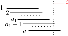
Figure 15: Illustrating the definition of $a_{1}$. The black segments show the positions of interval $m$ in the configurations $\mathcal{C}_{L_{j}^{\prime}}$ for $j\in[1,a]$, and the numbers on the left side are the indices of the lists. The red segment shows the interval $i$ in the input position.

Now consider the value $\delta(\mathcal{C}_{L_{j}})$, which is equal to $\max\{\delta(\mathcal{C}_{L^{\prime}_{j}}),d(i,\mathcal{C}_{L_{j}})\}$ by Observation 1. Recall that $\delta(\mathcal{C}_{L^{\prime}_{j}})$ is strictly decreasing on $j\in[1,a]$. Observe that $d(i,\mathcal{C}_{L_{j}})$ is $0$ on $j\in[1,a_{1}]$ and strictly increases on $j\in[a_{1},a]$. This implies that $\delta(\mathcal{C}_{L_{j}})$ on $j\in[1,a]$ is a unimodal function, i.e., it first strictly decreases and then strictly increases after some index, say, $a_{2}$. Formally, let $a_{2}$ be the largest index $j\in[a_{1}+1,a]$ such that $\delta(\mathcal{C}_{L_{j-1}})>\delta(\mathcal{C}_{L_{j}})$, and if no such index $j$ exists, then let $a_{2}=a_{1}$. The following lemma is proved based on Lemma 9.

Lemma 11

1. If $a_{1}>1$, then for each $j\in[1,a_{1}-1]$, $L_{a_{1}}$ dominates $L_{j}$.

2. If $a_{2}<a$, then for each $j\in[a_{2}+1,a]$, $L_{a_{2}}$ dominates $L_{j}$.

Proof

1. Let $k=a_{1}$ and assume $k>1$. Consider any $j\in[1,k-1]$. By the definition of $a_{1}$, $x_{i}^{l}(\mathcal{C}_{L_{j}})=x_{i}^{l}(\mathcal{C}_{L_{k}})=x_{i}^{l}$. Therefore, $x(\mathcal{C}_{L_{j}})=x(\mathcal{C}_{L_{k}})=x_{i}^{l}+|I_{i}|$. Since $d(i,\mathcal{C}_{L_{j}})=d(i,\mathcal{C}_{L_{k}})=0$, we have $\delta(\mathcal{C}_{L_{j}})=\delta(\mathcal{C}_{L^{\prime}_{j}})$ and $\delta(\mathcal{C}_{L_{k}})=\delta(\mathcal{C}_{L^{\prime}_{k}})$. Since $j<k$, $\delta(\mathcal{C}_{L^{\prime}_{j}})>\delta(\mathcal{C}_{L^{\prime}_{k}})$. Thus, we obtain $\delta(\mathcal{C}_{L_{j}})>\delta(\mathcal{C}_{L_{k}})$.

   Since $x(\mathcal{C}_{L_{j}})=x(\mathcal{C}_{L_{k}})$, $\delta(\mathcal{C}_{L_{j}})>\delta(\mathcal{C}_{L_{k}})$, and the last indices of $L_{j}$ and $L_{k}$ are both $i$, by Lemma 9, $L_{k}$ dominates $L_{j}$.

2. Let $k=a_{2}$ and assume $k<a$. Consider any $j\in[k+1,a]$. As discussed before, $x(\mathcal{C}_{L_{j}})$ is monotonically increasing on $j\in[1,a]$. Thus, $x(\mathcal{C}_{L_{k}})\leq x(\mathcal{C}_{L_{j}})$. By the definition of $a_{2}$ and since $\delta(\mathcal{C}_{L_{j}})$ is a unimodal function on $j\in[1,a]$, it holds that $\delta(\mathcal{C}_{L_{k}})\leq\delta(\mathcal{C}_{L_{j}})$. By Lemma 9, $L_{k}$ dominates $L_{j}$.

This proves the lemma. ∎

By Lemma 11, we let $\mathcal{L}=\{L_{j}\ |\ a_{1}\leq j\leq a_{2}\}$. The above is for the general case where $a_{1}\neq 0$. If $a_{1}=0$, then we let $\mathcal{L}=\{L_{j}\ |\ 1\leq j\leq a_{2}\}$.

Observation 4

All algorithm invariants hold for $\mathcal{L}$.

Proof

By Lemma 11, the lists that have been removed are redundant. Hence, $\mathcal{L}$ contains a canonical list of $\mathcal{I}[1,i]$ and the first algorithm invariant holds.

By our definitions of $a_{1}$ and $a_{2}$, when $j$ increases in $[a_{1},a_{2}]$, $x(\mathcal{C}_{L_{j}})$ strictly increases and $\delta(\mathcal{C}_{L_{j}})$ strictly decreases. Therefore, the last three algorithm invariants hold. ∎

The following lemma will be quite useful for the algorithm implementation given later in Section 5.3.

Lemma 12

If $a_{1}<a_{2}$, then for each $j\in[a_{1}+1,a_{2}]$, $x(\mathcal{C}_{L_{j}})=x(\mathcal{C}_{L^{\prime}_{j}})+|I_{i}|$. For each list $L_{j}\in\mathcal{L}$ with $j\neq a_{2}$, $\delta(\mathcal{C}_{L_{j}})=\delta(\mathcal{C}_{L^{\prime}_{j}})$.

Proof

By the definition of $a_{1}$, for any $j\in[a_{1}+1,a]$, it always holds that $x(\mathcal{C}_{L_{j}})=x(\mathcal{C}_{L^{\prime}_{j}})+|I_{i}|$. This proves the first lemma statement.

Recall that $\delta(\mathcal{C}_{L_{j}})=\max\{\delta(\mathcal{C}_{L^{\prime}_{j}}),d(i,\mathcal{C}_{L_{j}})\}$ for each $j\in[1,a]$.

Consider any list $L_{j}$ with $j\neq a_{2}$. Assume to the contrary that $\delta(\mathcal{C}_{L_{j}})\neq\delta(\mathcal{C}_{L^{\prime}_{j}})$. Then, $\delta(\mathcal{C}_{L_{j}})=d(i,\mathcal{C}_{L_{j}})$. Since $\delta(\mathcal{C}_{L_{j}})=d(i,\mathcal{C}_{L_{j}})<d(i,\mathcal{C}_{L_{a_{2}}})$, we obtain $\delta(\mathcal{C}_{L_{j}})\leq\delta(\mathcal{C}_{L_{a_{2}}})$, which contradicts with $\delta(\mathcal{C}_{L_{j}})>\delta(\mathcal{C}_{L_{a_{2}}})$. ∎

The second subcase $x_{m}^{r}>x_{i}^{r}$.

In this case, for each list $L_{j}^{\prime}\in\mathcal{L}^{\prime}$, according to our preliminary algorithm, depending on whether $x_{i}^{l}\leq x_{m}^{l}(\mathcal{C}_{L^{\prime}_{j}})$, either Case II or Case III can happen. If $x_{i}^{l}\leq x_{m}^{l}(\mathcal{C}_{L^{\prime}_{1}})$, then let $c=0$; otherwise, let $c$ be the largest index $j$ such that $x_{i}^{l}>x_{m}^{l}(\mathcal{C}_{L^{\prime}_{j}})$ (e.g., see Fig. 16). In the following, we first consider the general case where $1\leq c<a$.

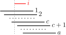
Figure 16: Illustrating the definition of $c$. The black segments show the positions of interval $m$ in the configurations $\mathcal{C}_{L_{j}^{\prime}}$ for $j\in[1,a]$, and the numbers on the right side are the indices of the lists. The red segment shows the interval $i$ in the input position.

For each $j\in[1,c]$, observe that $x_{m}^{l}(\mathcal{C}_{L^{\prime}_{j}})=x(\mathcal{C}_{L^{\prime}_{j}})-|I_{m}|\leq x(\mathcal{C}_{L^{\prime}_{c}})-|I_{m}|=x_{m}^{l}(\mathcal{C}_{L^{\prime}_{c}})<x_{i}^{l}$. According to our preliminary algorithm, Case III happens, and thus $L_{j}^{\prime}$ will produce two lists: the list $L_{j}$ by appending $i$ at the end of $L_{j}^{\prime}$, and the new list $L_{j}^{*}$ by inserting $i$ in front of $m$ in $L_{j}^{\prime}$. Further, according to our left-possible placement strategy, $x^{l}_{i}(\mathcal{C}_{L_{j}})=x(\mathcal{C}_{L_{j}^{\prime}})$ in $\mathcal{C}_{L_{j}}$, and $x^{l}_{i}(\mathcal{C}_{L^{*}_{j}})=x^{l}_{i}$ and $x^{l}_{m}(\mathcal{C}_{L^{*}_{j}})=x^{r}_{i}$ in $\mathcal{C}_{L^{*}_{j}}$. By Observation 3, $\delta(\mathcal{C}_{L_{j}})=\max\{\delta(\mathcal{C}_{L_{j}^{\prime}}),d(i,\mathcal{C}_{L_{j}})\}$ and $\delta(\mathcal{C}_{L^{*}_{j}})=\max\{\delta(\mathcal{C}_{L_{j}^{\prime}}),d(m,\mathcal{C}_{L^{*}_{j}})\}$.

Observation 5

$\delta(\mathcal{C}_{L^{*}_{c}})\leq\delta(\mathcal{C}_{L^{*}_{j}})$ for any $j\in[1,c]$.

Proof

For any $j\in[1,c]$, note that $d(m,\mathcal{C}_{L^{*}_{j}})=x^{l}_{m}(\mathcal{C}_{L^{*}_{j}})-x_{m}^{l}=x_{i}^{r}-x_{m}^{l}$. Therefore, $d(m,\mathcal{C}_{L^{*}_{j}})$ is the same for all $j\in[1,c]$. On the other hand, we have $\delta(\mathcal{C}_{L^{\prime}_{j}})\geq\delta(\mathcal{C}_{L^{\prime}_{c}})$. Thus, $\delta(\mathcal{C}_{L^{*}_{c}})\leq\delta(\mathcal{C}_{L^{*}_{j}})$. ∎

By the above observation and Lemma 6, among the new lists $L_{j}^{*}$ with $j=1,2,\ldots,c$, only $L_{c}^{*}$ needs to be kept.

For each $j\in[1,c]$, note that $x(\mathcal{C}_{L_{j}})=x(\mathcal{C}_{L_{j}^{\prime}})+|I_{i}|$. Since $x(\mathcal{C}_{L_{j}^{\prime}})$ is strictly increasing on $j\in[1,c]$, $x(\mathcal{C}_{L_{j}})$ is also strictly increasing on $j\in[1,c]$. Since $d(i,\mathcal{C}_{L_{j}})=x^{l}_{i}(\mathcal{C}_{L_{j}})-x_{i}^{l}=x(\mathcal{C}_{L_{j}^{\prime}})-x_{i}^{l}$ for any $j\in[1,c]$, $d(i,\mathcal{C}_{L_{j}})$ also strictly increases on $j\in[1,c]$. Further, since $\delta(\mathcal{C}_{L^{\prime}_{j}})$ strictly decreases on $j\in[1,c]$, $\delta(\mathcal{C}_{L_{j}})$, which is equal to $\max\{\delta(\mathcal{C}_{L_{j}^{\prime}}),d(i,\mathcal{C}_{L_{j}})\}$, is a unimodal function (i.e., it first strictly decreases and then strictly increases). Let $c_{1}$ be the smallest index $j\in[1,c-1]$ such that $\delta(\mathcal{C}_{L_{j}})\leq\delta(\mathcal{C}_{L_{j+1}})$, and if such an index $j$ does not exist, then let $c_{1}=c$.

Lemma 13

If $c_{1}<c$, then $L_{c_{1}}$ dominates $L_{j}$ for any $j\in[c_{1}+1,c]$.

Proof

Consider any $j\in[c_{1}+1,c]$. Since $\delta(\mathcal{C}_{L_{j}})$ is a unimodal function on $j\in[1,c]$, by the definition of $c_{1}$, $\delta(\mathcal{C}_{L_{c_{1}}})\leq\delta(\mathcal{C}_{L_{j}})$. Recall that $x(\mathcal{C}_{L_{c_{1}}})\leq x(\mathcal{C}_{L_{j}})$. Since the last indices of $L_{c_{1}}$ and $L_{j}$ are both $i$, by Lemma 9, $L_{c_{1}}$ dominates $L_{j}$. ∎

By the preceding lemma, if $c_{1}<c$, then we do not have to keep the lists $L_{c_{1}+1},\ldots,L_{c}$ in $\mathcal{L}$. Let $S_{1}=\{L_{1},\ldots,L_{c_{1}}\}$.

Consider any index $j\in[c+1,a]$. By the definition of $c$ and also due to that $x(\mathcal{C}_{L_{k}^{\prime}})$ is strictly increasing on $k\in[1,a]$, it holds that $x_{m}^{l}(\mathcal{C}_{L_{j}^{\prime}})\geq x_{i}^{l}$, and thus Case II of the preliminary algorithm happens on $L_{j}^{\prime}$ and $L_{j}$ is obtained by inserting $i$ right before $m$ in $L_{j}^{\prime}$. By Observation 2, $\delta(\mathcal{C}_{L_{j}})=\max\{\delta(\mathcal{C}_{L^{\prime}_{j}}),d(m,\mathcal{C}_{L_{j}})\}$. Note that $x(\mathcal{C}_{L_{j}})=x(\mathcal{C}_{L^{\prime}_{j}})+|I_{i}|$ and $x_{m}^{r}(\mathcal{C}_{L_{j}})=x(\mathcal{C}_{L_{j}})$. As $j$ increases in $[c+1,a]$, since $x(\mathcal{C}_{L_{j}^{\prime}})$ strictly increases, both $x(\mathcal{C}_{L_{j}})$ and $d(m,\mathcal{C}_{L_{j}})$ strictly increase. Since $\delta(\mathcal{C}_{L^{\prime}_{j}})$ is strictly decreasing on $j\in[c+1,a]$, we obtain that $\delta(\mathcal{C}_{L_{j}})$ is a unimodal function on $j\in[c+1,a]$ (i.e., it first strictly decreases and then strictly increases).

Let $S=\{L_{1},\ldots,L_{c},L_{c}^{*},L_{c+1},\ldots,L_{a}\}$. For convenience, we use $L_{c+0.5}$ to refer to $L_{c}^{*}$ (and $L^{\prime}_{c+0.5}$ refers to $L^{\prime}_{c}$); in this way, the indices of the ordered lists of $S$ are sorted. Consider the subsequence of the lists of $S$ from $L_{c+0.5}$ to the end (including $L_{c+0.5}$). Define $c_{2}$ to be the index of the first list $L_{j}$ such that $\delta(\mathcal{C}_{L_{j}})\leq\delta(\mathcal{C}_{L})$, where $L$ is the right neighboring list of $L_{j}$ in $S$; if such a list $L_{j}$ does not exist, then we let $c_{2}=a$.

Observation 6

As $j$ increases in $[1,a]$, $x(\mathcal{C}_{L_{j}})$ is strictly increasing except that $x(\mathcal{C}_{L_{c+0.5}})=x(\mathcal{C}_{L_{c+1}})$ may be possible.

Proof

Recall that $x(\mathcal{C}_{L_{j}})$ is strictly increasing on $j\in[1,c]$ and $j\in[c+1,a]$, respectively. Let $l=|I_{i}|+|I_{m}|$. Note that $x(\mathcal{C}_{L_{c}})=x_{m}^{l}(\mathcal{C}_{L^{\prime}_{c}})+l$, $x(\mathcal{C}_{L^{*}_{c}})=x^{l}_{i}+l$, and $x(\mathcal{C}_{L_{c+1}})=x^{l}_{m}(\mathcal{C}_{L^{\prime}_{c+1}})+l$. By our definition of $c$, $x^{l}_{m}(\mathcal{C}_{L^{\prime}_{c}})<x^{l}_{i}\leq x^{l}_{m}(\mathcal{C}_{L^{\prime}_{c+1}})$. Thus, $x(\mathcal{C}_{L_{c}})<x(\mathcal{C}_{L^{*}_{c}})\leq x(\mathcal{C}_{L_{c+1}})$. This shows that $x(\mathcal{C}_{L_{j}})$ is strictly increasing on $j\in[1,a]$ except that $x(\mathcal{C}_{L^{*}_{c}})=x(\mathcal{C}_{L_{c+1}})$ may be possible. ∎

Lemma 14

1. If $c_{2}<a$, then $L_{c_{2}}$ dominates $L_{j}$ for any $L_{j}\in S$ with $j>c_{2}$.

2. If $c_{2}\geq c+1$ and $x(\mathcal{C}_{L_{c+0.5}})=x(\mathcal{C}_{L_{c+1}})$, then $L_{c+1}$ dominates $L_{c+0.5}$.

Proof

We first show that $\delta(\mathcal{C}_{L_{j}})$ is a unimodal function on $j\in[c+0.5,a]$.

Recall that for each $j\in[c+1,a]$, $\delta(\mathcal{C}_{L_{j}})=\max\{\delta(\mathcal{C}_{L^{\prime}_{j}}),d(m,\mathcal{C}_{L_{j}})\}$, and $\delta(\mathcal{C}_{L^{*}_{j}})=\max\{\delta(\mathcal{C}_{L^{\prime}_{j}}),d(m,\mathcal{C}_{L^{*}_{j}})\}$. For each $j\in[c+0.5,a]$, since $m$ is the last index of $L_{j}$, we have $d(m,\mathcal{C}_{L_{j}})=x(\mathcal{C}_{L_{j}})-x_{m}^{r}$. By Observation 6, $d(m,\mathcal{C}_{L_{j}})$ is strictly increasing on $[c+0.5,a]$ except that $d(m,\mathcal{C}_{L_{c+0.5}})=d(m,\mathcal{C}_{L_{c+1}})$ may be possible. Since $\delta(\mathcal{C}_{L^{\prime}_{j}})$ on $j\in[1,a]$ is strictly decreasing, $\delta(\mathcal{C}_{L_{j}})$ is a unimodal function on $j\in[c+0.5,a]$.

By the definition of $c_{2}$, $\delta(\mathcal{C}_{L_{j}})$ is strictly decreasing on $[c+0.5,c_{2}]$ and monotonically increasing on $[c_{2},a]$.

Consider any list $L_{j}\in S$ with $j>c_{2}$. By our previous discussion, $\delta(\mathcal{C}_{L_{c_{2}}})\leq\delta(\mathcal{C}_{L_{j}})$ and $x(\mathcal{C}_{L_{c_{2}}})\leq x(\mathcal{C}_{L_{j}})$. Since the last indices of both $L_{c_{2}}$ and $L_{j}$ are $m$, by Lemma 9, $L_{c_{2}}$ dominates $L_{j}$.

If $c_{2}\geq c+1$ and $x(\mathcal{C}_{L_{c+0.5}})=x(\mathcal{C}_{L_{c+1}})$, by the definition of $c_{2}$, $\delta(\mathcal{C}_{L_{c+0.5}})>\delta(\mathcal{C}_{L_{c+1}})$. Since the last indices of both $L_{c+0.5}$ and $L_{c+1}$ are $m$, by Lemma 9, $L_{c+1}$ dominates $L_{c+0.5}$. The lemma thus follows. ∎

Let $S_{2}=\{L_{c+0.5},L_{c+1},\ldots,L_{c_{2}}\}$ and we remove $L_{c+0.5}$ from $S_{2}$ if $c_{2}\geq c+1$ and $x(\mathcal{C}_{L_{c+0.5}})=x(\mathcal{C}_{L_{c+1}})$. In the following, we combine $S_{1}$ and $S_{2}$ to obtain the set $\mathcal{L}$. We consider the lists of $S_{2}$ in order. Define $c^{\prime}$ to be the index $j$ of the first list $L_{j}$ such that $\delta(\mathcal{C}_{L_{c_{1}}})>\delta(\mathcal{C}_{L_{j}})$, and if no such list $L_{j}$ exists, then let $c^{\prime}=c_{2}+1$.

Lemma 15

If $L_{c^{\prime}}$ is not the first list of $S_{2}$ or $c^{\prime}=c_{2}+1$, then for each list $L_{j}$ of $S_{2}$ with $j<c^{\prime}$, $L_{c_{1}}$ dominates $L_{j}$.

Proof

We assume that $L_{c^{\prime}}$ is not the first list of $S_{2}$ or $c^{\prime}=c_{2}+1$.

Note that we have proved in the proof of Lemma 14 that $\delta(\mathcal{C}_{L_{j}})$ on $j\in[c+0.5,c_{2}]$ is strictly decreasing. By the definition of $c^{\prime}$, it holds that $\delta(\mathcal{C}_{L_{c_{1}}})\leq\delta(\mathcal{C}_{L_{j}})$ for any $L_{j}\in S_{2}$ with $j<c^{\prime}$.

Consider any list $L_{j}$ of $S_{2}$ with $j<c^{\prime}$.

Recall that $\delta(\mathcal{C}_{L_{j}})=\max\{\delta(\mathcal{C}_{L^{\prime}_{j}}),d(m,\mathcal{C}_{L_{j}})\}$. We claim that $\delta(\mathcal{C}_{L_{j}})=d(m,\mathcal{C}_{L_{j}})$. Indeed, note that $\delta(\mathcal{C}_{L_{j}^{\prime}})\leq\delta(\mathcal{C}_{L^{\prime}_{c_{1}}})\leq\delta(\mathcal{C}_{L_{c_{1}}})$. Since $\delta(\mathcal{C}_{L_{c_{1}}})\leq\delta(\mathcal{C}_{L_{j}})$, we obtain $\delta(\mathcal{C}_{L^{\prime}_{j}})\leq\delta(\mathcal{C}_{L_{j}})$, and thus, $\delta(\mathcal{C}_{L_{j}})=d(m,\mathcal{C}_{L_{j}})$.

Consequently, we have $\delta(\mathcal{C}_{L_{c_{1}}})\leq d(m,\mathcal{C}_{L_{j}})$ and $x(\mathcal{C}_{L_{c_{1}}})\leq x(\mathcal{C}_{L_{j}})$ (by Observation 6). Further, the last index of $L_{c_{1}}$ is $i$ and the last index of $L_{j}$ is $m$, with $x_{i}^{r}\leq x_{m}^{r}$. By Lemma 8, $L_{c_{1}}$ dominates $L_{j}$.

The lemma thus follows. ∎

We remove from $S_{2}$ all lists $L_{j}$ with $j<c^{\prime}$, and let $\mathcal{L}=S_{1}\cup S_{2}$. In general, if $c^{\prime}\neq c_{2}+1$, then $\mathcal{L}=\{L_{1},\ldots,L_{c_{1}},L_{c^{\prime}},\ldots,L_{c_{2}}\}$; otherwise, $\mathcal{L}=\{L_{1},\ldots,L_{c_{1}}\}$.

The above discussion is for the general case where $1\leq c<a$. If $c=0$, then $L_{c}^{*}$, $c_{1}$ and $c^{\prime}$ are all undefined, and we have $\mathcal{L}=\{L_{1},\ldots,L_{c_{2}}\}$. If $c=a$, then $\mathcal{L}=\{L_{1},\ldots,L_{c_{1}}\}$ if $\delta(L_{c_{1}})\leq\delta(L_{c}^{*})$ and $\mathcal{L}=\{L_{1},\ldots,L_{c_{1}},L_{c}^{*}\}$ otherwise.

Observation 7

All algorithm invariants hold on $\mathcal{L}$.

Proof

We only consider the most general case where $1\leq c<a$ and $c^{\prime}\neq c_{2}+1$, since other cases can be proved in a similar but easier way.

By Lemmas 13, 14, and 15, all pruned lists are redundant and thus $\mathcal{L}$ contains a canonical list of $\mathcal{I}[1,i]$. The first algorithm invariant holds.

If $x(\mathcal{C}_{L_{c+0.5}})=x(\mathcal{C}_{L_{c+1}})$, then $L_{c+0.5}$ and $L_{c+1}$ cannot be both in $\mathcal{L}$ by Lemma 14(2). Thus, by Observation 6, $x(\mathcal{C}_{L_{j}})$ strictly increases in $[1,a]$. Recall that for any list $L_{j}\in\mathcal{L}$, the last index of $L_{j}$ is $i$ if $j\leq c_{1}$ and $m$ otherwise. Recall that $I_{i}$ is contained in $I_{m}$ in the input. Thus, the fourth algorithm invariant holds.

Further, our definitions of $c_{1}$, $c^{\prime}$, and $c_{2}$ guarantee that $\delta(\mathcal{C}_{L})$ on all lists $L$ following their order in $\mathcal{L}$ is strictly decreasing. Therefore, the other two algorithm invariants also hold. ∎

The following lemma will be useful for the algorithm implementation.

Lemma 16

For each list $L_{j}\in\mathcal{L}$, if $L_{j}\neq L_{c}^{*}$, then $x(\mathcal{C}_{L_{j}})=x(\mathcal{C}_{L^{\prime}_{j}})+|I_{i}|$; if $L_{j}\not\in\{L_{c}^{*},L_{c_{1}},L_{c_{2}}\}$, then $\delta(\mathcal{C}_{L_{j}})=\delta(\mathcal{C}_{L^{\prime}_{j}})$.

Proof

If $L_{j}\neq L_{c}^{*}$, then we have discussed before that $x(\mathcal{C}_{L_{j}})=x(\mathcal{C}_{L^{\prime}_{j}})+|I_{i}|$ always holds regardless of whether the last index of $L_{j}$ is $i$ or $m$.

If $L_{j}\not\in\{L_{c}^{*},L_{c_{1}},L_{c_{2}}\}$, assume to the contrary that $\delta(\mathcal{C}_{L_{j}})\neq\delta(\mathcal{C}_{L^{\prime}_{j}})$. Then, since $\delta(\mathcal{C}_{L_{j}})=\max\{\delta(\mathcal{C}_{L^{\prime}_{j}}),d(k,\mathcal{C}_{L_{j}})\}$, we obtain that $\delta(\mathcal{C}_{L_{j}})=d(k,\mathcal{C}_{L_{j}})$, where $k$ is the last index of $\mathcal{C}_{L_{j}}$ ($k$ is $i$ if $j\leq c$ and $m$ otherwise). Note that $j$ is either in $[1,c_{1}]$ or $[c^{\prime},c_{2}]$. We discuss the two cases below.

1. If $j\in[1,c_{1}]$, then the last index of $L_{j}$ is $i$. Since $L_{j}\neq L_{c_{1}}$, $j<c_{1}$ holds. We have discussed before that $d(i,\mathcal{C}_{L_{j}})\leq d(i,\mathcal{C}_{L_{c_{1}}})$. Thus, we can deduce $\delta(\mathcal{C}_{L_{j}})=d(i,\mathcal{C}_{L_{j}})\leq d(i,\mathcal{C}_{L_{c_{1}}})\leq\delta(\mathcal{C}_{L_{c_{1}}})$. However, we have already proved that $\delta(\mathcal{C}_{L_{j}})>\delta(\mathcal{C}_{L_{c_{1}}})$. Thus, we obtain contradiction.

2. If $j\in[c^{\prime},c_{2}]$, the analysis is similar. In this case the last index of $L_{j}$ is $m$ and $j<c_{2}$. Since $j<c_{2}$, we have discussed before that $d(m,\mathcal{C}_{L_{j}})\leq d(m,\mathcal{C}_{L_{c_{2}}})$. Thus, we can deduce $\delta(\mathcal{C}_{L_{j}})=d(m,\mathcal{C}_{L_{j}})\leq d(m,\mathcal{C}_{L_{c_{2}}})\leq\delta(\mathcal{C}_{L_{c_{2}}})$. However, we have already proved that $\delta(\mathcal{C}_{L_{j}})>\delta(\mathcal{C}_{L_{c_{2}}})$. Thus, we obtain contradiction.

The lemma thus follows. ∎

5.2.2 The Case $\mathcal{L}_{1}^{\prime}\neq\emptyset$

We then consider the case where $\mathcal{L}_{1}^{\prime}\neq\emptyset$. In this case, recall that $\mathcal{L}_{1}^{\prime}=\{L_{1}^{\prime},\ldots,L_{b}^{\prime}\}$ and $\mathcal{L}_{2}^{\prime}=\{L_{b+1}^{\prime},\ldots,L_{a}^{\prime}\}$. For each $L^{\prime}_{j}\in\mathcal{L}^{\prime}$, the last index of $L^{\prime}_{j}$ is $m^{\prime}$ if $j\leq b$ and $m$ otherwise. Recall that $I_{m^{\prime}}\subseteq I_{m}$ in the input. As in the proof of Lemma 10, there are three subcases: $x_{i}^{r}\geq x_{m}^{r}$, $x_{m^{\prime}}^{r}\leq x_{i}^{r}<x_{m}^{r}$, and $x_{i}^{r}<x_{m^{\prime}}^{r}$.

The first subcase $x_{i}^{r}\geq x_{m}^{r}$.

In this case, for each $L_{j}^{\prime}\in\mathcal{L}^{\prime}$, Case I of the preliminary algorithm happens and $L_{j}$ is obtained by appending $i$ at the end of $L_{j}^{\prime}$. Our pruning procedure for this subcase is similar to the first subcase in Section 5.2.1, and we briefly discuss it below.

First, for each $L_{j}^{\prime}\in\mathcal{L}^{\prime}$, $x_{i}^{l}(\mathcal{C}_{L_{j}})=\max\{x(\mathcal{C}_{L^{\prime}_{j}}),x_{i}^{l}\}$ and $\delta(\mathcal{C}_{L_{j}})=\max\{\delta(\mathcal{C}_{L^{\prime}_{j}}),d(i,\mathcal{C}_{L_{j}})\}$. We define $a_{1}$ and $a_{2}$ in exactly the same way as in the first subcase of Section 5.2.1, and further, Lemma 11 still holds. Similarly, we let $\mathcal{L}$ consist of only those lists $L_{j}$ with $j\in[a_{1},a_{2}]$. By the similar analysis, Observation 4 and Lemma 12 still hold. We omit the details.

The second subcase $x_{m^{\prime}}^{r}\leq x_{i}^{r}<x_{m}^{r}$.

In this case, we first apply the similar pruning procedure for the first (resp., second) subcase of Section 5.2.1 to set $\mathcal{L}_{1}^{\prime}$ (resp., $\mathcal{L}_{2}^{\prime}$), and then we combine the results. The details are given below.

For set $\mathcal{L}_{1}^{\prime}$, the last indices of all lists of $\mathcal{L}_{1}^{\prime}$ are $m^{\prime}$. Since $x_{m^{\prime}}^{r}\leq x_{i}^{r}$, for each $L_{j}^{\prime}\in\mathcal{L}^{\prime}_{1}$, Case I of the preliminary algorithm happens and $L_{j}$ is obtained by appending $i$ at the end of $L_{j}^{\prime}$. We define $a_{1}$ and $a_{2}$ in the similar way as in the first subcase of Section 5.2.1 but with respect to the indices in $[1,b]$. In fact, since $x_{i}^{r}<x_{m}^{r}$, it holds that $x_{i}^{l}\leq x_{i}^{r}\leq x_{m}^{r}\leq x(\mathcal{C}_{L^{\prime}_{1}})$, and consequently, $a_{1}=0$. Similarly, Lemma 11 also holds with respect to the indices of $[1,b]$. Further, as $j$ increases in $[1,a_{2}]$, $x(\mathcal{C}_{L_{j}})$ is strictly increasing and $\delta(\mathcal{C}_{L_{j}})$ is strictly decreasing. Let $S^{\prime}_{1}=\{L_{1},L_{2},\ldots,L_{a_{2}}\}$.

For set $\mathcal{L}_{2}^{\prime}$, the last indices of all its lists are $m$. Since $x_{i}^{r}<x_{m}^{r}$, for each list $L_{j}^{\prime}\in\mathcal{L}_{2}$, either Case II or Case III of the algorithm happens. We define $c$ in the similar way as in the second subcase of Section 5.2.1 but with respect to the indices of $[b+1,a]$. Specifically, if $x_{i}^{l}\leq x_{m}^{l}(\mathcal{C}_{L^{\prime}_{b+1}})$, then let $c=b$; otherwise, let $c$ be the largest index $j\in[b+1,a]$ such that $x_{i}^{l}>x_{m}^{l}(\mathcal{C}_{L^{\prime}_{j}})$. We consider the most general case where $b+1\leq c<a$ (other cases are similar but easier).

For each $j\in[b+1,c]$, there is also a new list $L^{*}_{j}$. Similar to Observation 4, $\delta(\mathcal{C}_{L^{*}_{c}})\leq\delta(\mathcal{C}_{L^{*}_{j}})$ for any $j\in[b+1,c]$. Hence, among the new lists $L_{j}^{*}$ with $j=b+1,\ldots,c$, only $L_{c}^{*}$ needs to be kept. Let $S^{\prime}=\{L_{b+1},\ldots,L_{c},L_{c}^{*},L_{c+1},\ldots,L_{a}\}$. We also use $L_{c+0.5}$ to refer to $L_{c}^{*}$. We define the three indices $c_{1}$, $c_{2}$, and $c^{\prime}$ in the similar way as in the second subcase of Section 5.2.1 but with respect to the ordered lists in $S^{\prime}$. Similarly, Observation 6, Lemmas 13, 14, and 15 all hold with respect to the lists in $S^{\prime}$. Let $S^{\prime}_{2}=\{L_{b+1},\ldots,L_{c_{1}},L_{c^{\prime}},\ldots,L_{c_{2}}\}$.

Finally, we combine the lists of the two sets $S^{\prime}_{1}$ and $S^{\prime}_{2}$ to obtain $\mathcal{L}$, as follows. Recall that $L_{a_{2}}$ is the last list of $S^{\prime}_{1}$. We consider the lists of $S_{2}^{\prime}$ in order. Define $b^{\prime}$ to be the index $j$ of the first list $L_{j}$ of $S_{2}^{\prime}$ such that $\delta(\mathcal{C}_{L_{a_{2}}})>\delta(\mathcal{C}_{L_{j}})$, and if no such list $L_{j}$ exists, then let $b^{\prime}=c_{2}+1$.

Lemma 17

1. $x(\mathcal{C}_{L_{a_{2}}})<x(\mathcal{C}_{L_{b+1}})$.

2. If $b^{\prime}>b+1$, then $L_{a_{2}}$ dominates $L_{j}$ for any list $L_{j}\in S_{2}^{\prime}$ with $j<b^{\prime}$.

Proof

For $L_{a_{2}}$, since $a_{1}=0$, we have $x(\mathcal{C}_{L_{a_{2}}})=x(\mathcal{C}_{L^{\prime}_{a_{2}}})+|I_{i}|$. For $L_{b+1}$, it holds that $x(\mathcal{C}_{L_{b+1}})=x(\mathcal{C}_{L^{\prime}_{b+1}})+|I_{i}|$. Since $x(\mathcal{C}_{L^{\prime}_{a_{2}}})<x(\mathcal{C}_{L^{\prime}_{b+1}})$, we have $x(\mathcal{C}_{L_{a_{2}}})<x(\mathcal{C}_{L_{b+1}})$. This proves the first statement of the lemma.

Next we prove the second lemma statement. Assume $b^{\prime}>b+1$. Consider any list $L_{j}\in S_{2}^{\prime}$ with $j<b^{\prime}$. In the following, we show that $L_{a_{2}}$ dominates $L_{j}$.

Recall that the values $\delta(L)$ of the lists $L$ of $S^{\prime}_{2}$ are strictly decreasing following their order in $S^{\prime}_{2}$. By the definition of $b^{\prime}$, $\delta(\mathcal{C}_{L_{a_{2}}})\leq\delta(\mathcal{C}_{L_{j}})$. Note that the last index of $L_{j}$ can be either $i$ or $m$, and the last index of $L_{a_{2}}$ is $i$.

If the last index of $L_{j}$ is $i$, then since $\delta(\mathcal{C}_{L_{a_{2}}})\leq\delta(\mathcal{C}_{L_{j}})$ and $x(\mathcal{C}_{L_{a_{2}}})<x(\mathcal{C}_{L_{b+1}})\leq x(\mathcal{C}_{L_{j}})$, by Lemma 9, $L_{a_{2}}$ dominates $L_{j}$.

If the last index of $L_{j}$ is $m$, then $\delta(\mathcal{C}_{L_{j}})=\max\{\delta(\mathcal{C}_{L^{\prime}_{j}}),d(m,\mathcal{C}_{L_{j}})\}$. Recall that $\delta(\mathcal{C}_{L_{a_{2}}})=\max\{\delta(\mathcal{C}_{L^{\prime}_{a_{2}}}),d(i,\mathcal{C}_{L_{a_{2}}})\}$ and $\delta(\mathcal{C}_{L^{\prime}_{a_{2}}})>\delta(\mathcal{C}_{L^{\prime}_{j}})$. Due to $\delta(\mathcal{C}_{L_{a_{2}}})\leq\delta(\mathcal{C}_{L_{j}})$, we can deduce $\delta(\mathcal{C}_{L^{\prime}_{j}})<\delta(\mathcal{C}_{L^{\prime}_{a_{2}}})\leq\delta(\mathcal{C}_{L_{a_{2}}})\leq\delta(\mathcal{C}_{L_{j}})$. Therefore, $\delta(\mathcal{C}_{L_{a_{2}}})\leq\delta(\mathcal{C}_{L_{j}})=d(m,\mathcal{C}_{L_{j}})$. Again, $x(\mathcal{C}_{L_{a_{2}}})<x(\mathcal{C}_{L_{b+1}})\leq x(\mathcal{C}_{L_{j}})$. Since the last index of $L_{a_{2}}$ is $i$ and that of $L_{j}$ is $m$, with $I_{i}\subseteq I_{m}$ in the input, by Lemma 8, $L_{a_{2}}$ dominates $L_{j}$. ∎

By Lemma 17, we let $\mathcal{L}$ be the union of the lists of $S^{\prime}_{1}$ and the lists of $S^{\prime}_{2}$ after and including $b^{\prime}$ (if $b^{\prime}=c_{2}+1$, then $\mathcal{L}=S_{1}^{\prime}$).

Observation 8

All algorithm invariants hold on $\mathcal{L}$.

Proof

As the analysis in Section 5.2.1, $S^{\prime}_{1}\cup S^{\prime}_{2}$ must contain a canonical list of $\mathcal{I}[1,i]$. In light of Lemma 17(2), $\mathcal{L}$ also contains a canonical list.

Also, the values of $x(\mathcal{C}_{L})$ for all lists $L$ of $S^{\prime}_{1}$ (resp., $S^{\prime}_{2}$) are strictly increasing. By Lemma 17(1), the values of $x(\mathcal{C}_{L})$ for all lists $L$ of $\mathcal{L}$ are also strictly increasing. On the other hand, the values of $\delta(\mathcal{C}_{L})$ for all lists $L$ of $S^{\prime}_{1}$ (resp., $S^{\prime}_{2}$) are strictly decreasing. The definition of $b^{\prime}$ makes sure that the values of $\delta(\mathcal{C}_{L})$ for all lists $L$ of $\mathcal{L}$ must be strictly decreasing. Also, note that the lists of $\mathcal{L}$ whose last indices are $i$ are all before the lists whose last indices are $m$.

Hence, all algorithm invariants hold on $\mathcal{L}$. ∎

The following lemma will be useful for the algorithm implementation.

Lemma 18

For each list $L_{j}\in\mathcal{L}$, if $L_{j}\neq L_{c}^{*}$, then $x(\mathcal{C}_{L_{j}})=x(\mathcal{C}_{L^{\prime}_{j}})+|I_{i}|$; if $L_{j}\not\in\{L_{a_{2}},L_{c}^{*},L_{c_{1}},L_{c_{2}}\}$, then $\delta(\mathcal{C}_{L_{j}})=\delta(\mathcal{C}_{L^{\prime}_{j}})$.

Proof

Consider any list $L_{j}\in\mathcal{L}$.

If $L_{j}\neq L_{c}^{*}$, then since $a_{1}=0$, $x(\mathcal{C}_{L_{j}})=x(\mathcal{C}_{L^{\prime}_{j}})+|I_{i}|$ always holds regardless whether the last index of $L_{j}$ is $i$ or $m$.

Assume $L_{j}\not\in\{L_{a_{2}},L_{c}^{*},L_{c_{1}},L_{c_{2}}\}$. To prove that $\delta(\mathcal{C}_{L_{j}})=\delta(\mathcal{C}_{L^{\prime}_{j}})$, if $j\leq b$, then we can apply the analysis in the proof of Lemma 12; otherwise, we can apply the analysis in the proof of Lemma 16. We omit the details. ∎

The third subcase $x_{i}^{r}<x_{m^{\prime}}^{r}$.

In this case, for each list $L_{j}^{\prime}\in\mathcal{L}^{\prime}$, as analyzed in the proof of Lemma 10, only Case II of our preliminary algorithm happens, and thus $L_{j}$ is obtained from $L_{j}^{\prime}$ by inserting $i$ into $L_{j}^{\prime}$ right before the last index. Further, it holds that $x(\mathcal{C}_{L_{j}})=x(\mathcal{C}_{L^{\prime}_{j}})+|I_{i}|$ regardless of whether the last index of $L_{j}^{\prime}$ is $m$ or $m^{\prime}$. Since $x(\mathcal{C}_{L^{\prime}_{j}})$ is strictly increasing on $j\in[1,a]$, $x(\mathcal{C}_{L_{j}})$ is also strictly increasing on $j\in[1,a]$.

Consider any list $L^{\prime}_{j}\in\mathcal{L}^{\prime}$ with $j\leq b$. Recall that the last index of $L^{\prime}_{j}$ is $m^{\prime}$. By Observation 2, $\delta(\mathcal{C}_{L_{j}})=\max\{\delta(\mathcal{C}_{L^{\prime}_{j}}),d(m^{\prime},\mathcal{C}_{L_{j}})\}$, and $d(m^{\prime},\mathcal{C}_{L_{j}})=x_{m^{\prime}}^{r}(\mathcal{C}_{L_{j}})-x_{m^{\prime}}^{r}=x(\mathcal{C}_{L_{j}})-x_{m^{\prime}}^{r}$. Thus, $d(m^{\prime},\mathcal{C}_{L_{j}})$ strictly increases on $j\in[1,b]$. Since $\delta(\mathcal{C}_{L^{\prime}_{j}})$ strictly decreases on $j\in[1,b]$, $\delta(\mathcal{C}_{L_{j}})$ is a unimodal function on $j\in[1,b]$ (i.e., it first strictly decreases and then strictly increases). If $\delta(\mathcal{C}_{L_{1}})\leq\delta(\mathcal{C}_{L_{2}})$, then let $e_{1}=1$; otherwise, define $e_{1}$ to be the largest index $j\in[2,b]$ such that $\delta(\mathcal{C}_{L_{j-1}})>\delta(\mathcal{C}_{L_{j}})$. Hence, $\delta(\mathcal{C}_{L_{j}})$ is strictly decreasing on $j\in[1,e_{1}]$.

Lemma 19

If $e_{1}<b$, then $L_{e_{1}}$ dominates $L_{j}$ for any $j\in[e_{1}+1,b]$.

Proof

Assume $e_{1}<b$ and let $j$ be any index in $[e_{1}+1,b]$. By our definition of $e_{1}$ and since $\delta(\mathcal{C}_{L_{j}})$ is unimodal on $[1,b]$, it holds that $\delta(\mathcal{C}_{L_{e_{1}}})\leq\delta(\mathcal{C}_{L_{j}})$. Recall that $x(\mathcal{C}_{L_{e_{1}}})<x(\mathcal{C}_{L_{j}})$. Since the last indices of both $L_{e_{1}}$ and $L_{j}$ are $m^{\prime}$, by Lemma 9, $L_{e_{1}}$ dominates $L_{j}$. ∎

Due to Lemma 19, let $S_{1}=\{L_{1},L_{2},\ldots,L_{e_{1}}\}$.

Consider any list $L^{\prime}_{j}\in\mathcal{L}^{\prime}$ with $j>b$. Recall that the last index of $L^{\prime}_{j}$ is $m$. Similarly as above, $\delta(\mathcal{C}_{L_{j}})=\max\{\delta(\mathcal{C}_{L^{\prime}_{j}}),d(m,\mathcal{C}_{L_{j}})\}$ and $d(m,\mathcal{C}_{L_{j}})=x(\mathcal{C}_{L_{j}})-x_{m}^{r}$. Similarly, $\delta(\mathcal{C}_{L_{j}})$ is a unimodal function on $j\in[b+1,a]$. If $\delta(\mathcal{C}_{L_{b+1}})\leq\delta(\mathcal{C}_{L_{b+2}})$, then we let $e_{2}=b+1$; otherwise, define $e_{2}$ to be the largest index $j\in[b+1,a]$ such that $\delta(\mathcal{C}_{L_{j-1}})>\delta(\mathcal{C}_{L_{j}})$. Hence, $\delta(\mathcal{C}_{L_{j}})$ is strictly decreasing on $j\in[b+1,e_{2}]$. By a similar proof as Lemma 19, we can show that if $e_{2}<a$, then $L_{e_{2}}$ dominates $L_{j}$ for any $j\in[e_{2}+1,a]$. Let $S_{2}=\{L_{b+1},L_{b+2},\ldots,L_{e_{2}}\}$.

We finally combine $S_{1}$ and $S_{2}$ to obtain $\mathcal{L}$ as follows. Define $b^{\prime}$ to be the smallest index $j$ of $[b+1,e_{2}]$ such that $\delta(\mathcal{C}_{L_{e_{1}}})>\delta(\mathcal{C}_{L_{j}})$, and if no such index exists, then let $b^{\prime}=e_{2}+1$.

Lemma 20

If $b^{\prime}>b+1$, then $L_{e_{1}}$ dominates $L_{j}$ of $S_{2}$ for any $j\in[b+1,b^{\prime}-1]$.

Proof

Assume $b^{\prime}>b+1$ and let $j$ be any index in $[b+1,b^{\prime}-1]$. Since $\delta(\mathcal{C}_{L_{j}})$ is strictly decreasing on $j\in[b+1,e_{2}]$, by the definition of $b^{\prime}$, $\delta(\mathcal{C}_{L_{e_{1}}})\leq\delta(\mathcal{C}_{L_{j}})$.

Recall that $\delta(\mathcal{C}_{L_{j}})=\max\{\delta(\mathcal{C}_{L^{\prime}_{j}}),d(m,\mathcal{C}_{L_{j}})\}$, $\delta(\mathcal{C}_{L_{e_{1}}})=\max\{\delta(\mathcal{C}_{L^{\prime}_{e_{1}}}),d(m^{\prime},\mathcal{C}_{L_{e_{1}}})\}$, and $\delta(\mathcal{C}_{L^{\prime}_{j}})<\delta(\mathcal{C}_{L^{\prime}_{e_{1}}})$. Hence, we obtain $\delta(\mathcal{C}_{L^{\prime}_{j}})<\delta(\mathcal{C}_{L^{\prime}_{e_{1}}})\leq\delta(\mathcal{C}_{L_{j}})$, and thus $\delta(\mathcal{C}_{L_{j}})=d(m,\mathcal{C}_{L_{j}})$. Since $\delta(\mathcal{C}_{L_{e_{1}}})\leq\delta(\mathcal{C}_{L_{j}})$, $\delta(\mathcal{C}_{L_{e_{1}}})\leq d(m,\mathcal{C}_{L_{j}})$. Further, recall that $x(\mathcal{C}_{L_{e_{1}}})<x(\mathcal{C}_{L_{j}})$. Then, Lemma 8 applies since the last index of $L_{e_{1}}$ is $m^{\prime}$ and that of $L_{j}$ is $m$, with $x_{m^{\prime}}^{r}\leq x_{m}^{r}$. By Lemma 8, $L_{e_{1}}$ dominates $L_{j}$. ∎

In light of Lemma 20, we let $\mathcal{L}=S_{1}\cup\{L_{b^{\prime}},\ldots,L_{e_{2}}\}$ if $b^{\prime}\neq e_{2}+1$ and $\mathcal{L}=S_{1}$ otherwise. By similar analysis as before, we can show that all algorithm invariants hold on $\mathcal{L}$, and we omit the details. The following lemma will be useful for the algorithm implementation.

Lemma 21

For each list $L_{j}\in\mathcal{L}$, $x(\mathcal{C}_{L_{j}})=x(\mathcal{C}_{L^{\prime}_{j}})+|I_{i}|$; if $L_{j}\not\in\{L_{e_{1}},L_{e_{2}}\}$, then $\delta(\mathcal{C}_{L_{j}})=\delta(\mathcal{C}_{L^{\prime}_{j}})$.

Proof

We have shown that $x(\mathcal{C}_{L_{j}})=x(\mathcal{C}_{L^{\prime}_{j}})+|I_{i}|$ for any $j\in[1,a]$.

Consider any list $L_{j}\in\mathcal{L}$ and $j\not\in\{e_{1},e_{2}\}$. By the similar analysis as in Lemma 16, we can show that $\delta(\mathcal{C}_{L_{j}})=\delta(\mathcal{C}_{L^{\prime}_{j}})$. The details are omitted. ∎

5.3 The Algorithm Implementation

In this section, we implement our pruning algorithm described in Section 5.2 in $O(n\log n)$ time and $O(n)$ space. We first show how to compute the optimal value $\delta_{opt}$ and then show how to construct an optimal list $L_{opt}$ in Section 5.4.

Since $\mathcal{L}$ may have $\Theta(n)$ lists and each list may have $\Theta(n)$ intervals, to avoid $\Omega(n^{2})$ time, the key idea is to maintain the lists of $\mathcal{L}$ implicitly. We show that it is sufficient to maintain the “$x$-values” $x(\mathcal{C}_{L})$ and the “$\delta$-values” $\delta(\mathcal{C}_{L})$ for all lists $L$ of $\mathcal{L}$, as well as the list index $b$ and the interval indices $m^{\prime}$ and $m$. To this end, and in particular, to update the $x$-values and the $\delta$-values after each interval $I_{i}$ is processed, our implementation heavily relies on Lemmas 12, 16, 18, and 21. Intuitively, these lemmas guarantee that although the $x$-values of all lists of $\mathcal{L}$ need to change, all but a constant number of them increase by the same amount, which can be updated implicitly in constant time; similarly, only a constant number of $\delta$-values need to be updated. The details are given below.

Let $\mathcal{L}=\{L_{1},L_{2},\ldots,L_{a}\}$ such that $x(\mathcal{C}_{L_{j}})$ strictly increases on $j\in[1,a]$, and thus, $\delta(\mathcal{C}_{L_{j}})$ strictly decreases on $j\in[1,a]$ by the algorithm invariants.

We maintain a balanced binary search tree $T$ whose leaves from left to right correspond to the ordered lists of $\mathcal{L}$. Let $v_{1},\ldots,v_{a}$ be the leaves of $T$ from left to right, and thus, $v_{j}$ corresponds to $L_{j}$ for each $j\in[1,a]$. For each $j\in[1,a]$, $v_{j}$ stores a $\delta$-value $\delta(v_{j})$ that is equal to $\delta(\mathcal{C}_{L_{j}})$, and $v_{j}$ stores another $x$-value $x(v_{j})$ that is equal to $x(\mathcal{C}_{L_{j}})-R$, where $R$ is a global shift value maintained by the algorithm.

In addition, we maintain a pointer $p_{b}$ pointing to the leaf $v(b)$ of $T$ if $b\neq 0$ and $p_{b}=null$ if $b=0$. We also maintain the interval indices $m$ and $m^{\prime}$. Again, if $p_{b}=null$, then $m^{\prime}$ is undefined.

Initially, after $I_{1}$ is processed, $\mathcal{L}$ consists of the single list $L=\{1\}$. We set $R=0$, $m=1$, and $p_{b}=null$. The tree $T$ consists of only one leaf $v_{1}$ with $\delta(v_{1})=0$ and $x(v_{1})=x_{1}^{r}$.

In general, we assume $I_{i-1}$ has been processed and $T$, $m$, $m^{\prime}$, $p_{b}$, and $R$ have been correctly maintained. In the following, we show how to update them for processing $I_{i}$. In particular, we show that processing $I_{i}$ takes $O((k+1)\log n)$ time, where $k$ is the number of lists removed from $\mathcal{L}$ during processing $I_{i}$. Since our algorithm will generate at most $n$ new lists for $\mathcal{L}$ and each list will be removed from $\mathcal{L}$ at most once, the total time of the algorithm is $O(n\log n)$.

As in Section 5.2, we let $\mathcal{L}^{\prime}=\{L_{1}^{\prime},L_{2}^{\prime},\ldots,L_{a}^{\prime}\}$ denote the original set $\mathcal{L}$ before $I_{i}$ is processed. Again, if $b\neq 0$, then $\mathcal{L}_{1}^{\prime}=\{L_{1}^{\prime},\ldots,L_{b}^{\prime}\}$ and $\mathcal{L}_{2}^{\prime}=\{L_{b+1}^{\prime},\ldots,L_{a}^{\prime}\}$. We consider the five subcases discussed in Section 5.2.

5.3.1 The Case $\mathcal{L}_{1}^{\prime}=\emptyset$

In this case, the last indices of all lists of $\mathcal{L}^{\prime}$ are $m$.

The first subcase $x_{m}^{r}\leq x_{i}^{r}$.

In this case, in general we have $\mathcal{L}=\{L_{j}\ |\ a_{1}\leq j\leq a_{2}\}$. We first find $a_{1}$ and remove the lists $L_{1},\ldots,L_{a_{1}-1}$ if $a_{1}>1$ as follows.

Starting from the leftmost leaf $v_{1}$ of $T$, if $x(v_{1})+R$ (which is equal to $x(\mathcal{C}_{L_{1}^{\prime}})$) is larger than $x_{i}^{l}$, then $a_{1}=0$ and we are done. Otherwise, we consider the next leaf $v_{2}$. In general, suppose we are considering leaf $v_{j}$. If $x(v_{j})+R>x_{i}^{l}$, then we stop with $a_{1}=j-1$. Otherwise, we remove leaf $v_{j-1}$ (not $v_{j}$) from $T$ and continue to consider the next leaf $v_{j+1}$ if $j\neq a$ (if $j=a$, then we stop with $a_{1}=a$).

If $a_{1}\neq 0$, then the above has found the leaf $v_{a_{1}}$. In addition, we update $x(v_{a_{1}})=x_{i}^{r}-R-|I_{i}|$ (we have minus $|I_{i}|$ here because later we will increase $R$ by $|I_{i}|$).

Next we find $a_{2}$ and remove the lists $L_{a_{2}+1},\ldots,L_{a}$ (by removing the corresponding leaves from $T$) if $a_{2}<a$, as follows. Recall that for each $j\in[a_{1}+1,a]$, $\delta(\mathcal{C}_{L_{j}})=\max\{\delta(\mathcal{C}_{L^{\prime}_{j}}),d(i,\mathcal{C}_{L_{j}})\}$, with $\delta(\mathcal{C}_{L^{\prime}_{j}})=\delta(v_{j})$ and $d(i,\mathcal{C}_{L_{j}})=x_{i}^{l}(\mathcal{C}_{L_{j}})-x_{i}^{l}=x(\mathcal{C}_{L^{\prime}_{j}})-x_{i}^{l}=x(v_{j})+R-x_{i}^{l}$. Hence, we have $\delta(\mathcal{C}_{L_{j}})=\max\{\delta(v_{j}),x(v_{j})+R-x_{i}^{l}\}$.

If $a_{1}=a$, then we have $a_{2}=a_{1}$ and we are done. Otherwise we do the following. Starting from the rightmost leaf $v_{a}$ of $T$, we check whether $\max\{\delta(v_{a-1}),x(v_{a-1})+R-x_{i}^{l}\}\leq\max\{\delta(v_{a}),x(v_{a})+R-x_{i}^{l}\}$. If yes, we remove $v_{a}$ from $T$ and continue to consider $v_{a-1}$. In general, suppose we are considering $v_{j}$. If $j=a_{1}$, then we stop with $a_{2}=a_{1}$. Otherwise, we check whether $\max\{\delta(v_{j-1}),x(v_{j-1})+R-x_{i}^{l}\}\leq\max\{\delta(v_{j}),x(v_{j})+R-x_{i}^{l}\}$. If yes, we remove $v_{j}$ from $T$ and proceed on $v_{j-1}$. Otherwise, we stop with $a_{2}=j$.

Suppose the above procedure finds leaf $v_{j}$ with $a_{2}=j$. We further update $\delta(v_{j})=\max\{\delta(v_{j}),x(v_{j})+R-x_{i}^{l}\}$. By Lemma 12, we do not need to update other $\delta$-values.

The above has updated the tree $T$. In addition, we update $R=R+|I_{i}|$, which actually implicitly updates all $x$-values by Lemma 12. Finally, we update $m=i$ since the last indices of all updated lists of $\mathcal{L}$ are now $i$.

This finishes our algorithm for processing $I_{i}$. Clearly, the total time is $O((k+1)\log n)$ since removing each leaf of $T$ takes $O(\log n)$ time, where $k$ is the number of leaves that have been removed from $T$.

The second subcase $x_{m}^{r}>x_{i}^{r}$.

In this case, roughly speaking, we should compute the set $\mathcal{L}=\{L_{1},\ldots,L_{c_{1}},L_{c^{\prime}},L_{c^{\prime}+1},\ldots,L_{c_{2}}\}$.

We first compute the index $c$, i.e., find the leaf $v_{c}$ of $T$. This can be done by searching $T$ in $O(\log n)$ time as follows. Note that for a list $L_{j}^{\prime}$, to check whether $x_{i}^{l}>x_{m}^{l}(\mathcal{C}_{L^{\prime}_{j}})$, since $x_{m}^{l}(\mathcal{C}_{L^{\prime}_{j}})=x(\mathcal{C}_{L^{\prime}_{j}})-|I_{m}|=x(v_{j})+R-|I_{m}|$, it is equivalent to checking whether $x_{i}^{l}>x(v_{j})+R-|I_{m}|$, which is equivalent to $x_{i}^{l}-R+|I_{m}|>x(v_{j})$. Consequently, $v_{c}$ is the rightmost leaf $v$ of $T$ such that $x_{i}^{l}-R+|I_{m}|>x(v)$, and thus $v_{c}$ can be found by searching $T$ in $O(\log n)$ time.

Next, we find $c_{1}$, and remove the leaves $v_{j}$ with $j\in[c_{1}+1,c]$ if $c_{1}<c$, as follows (note that if the above step finds $c=0$, then we skip this step).

Recall that for each $j\in[1,c]$, $\delta(\mathcal{C}_{L_{j}})=\max\{\delta(\mathcal{C}_{L^{\prime}_{j}}),d(i,\mathcal{C}_{L_{j}})\}$, with $\delta(\mathcal{C}_{L^{\prime}_{j}})=\delta(v_{j})$ and $d(i,\mathcal{C}_{L_{j}})=x_{i}^{l}(\mathcal{C}_{L_{j}})-x_{i}^{l}=x(\mathcal{C}_{L^{\prime}_{j}})-x_{i}^{l}=x(v_{j})+R-x_{i}^{l}$. Hence, we have $\delta(\mathcal{C}_{L_{j}})=\max\{\delta(v_{j}),x(v_{j})+R-x_{i}^{l}\}$.

Starting from $v_{c}$, we first check whether $\delta(\mathcal{C}_{L_{c-1}})>\delta(\mathcal{C}_{L_{c}})$, by computing $\delta(\mathcal{C}_{L_{c-1}})$ and $\delta(\mathcal{C}_{L_{c}})$ as above. If yes, then $c_{1}=c$ and we stop. Otherwise, we remove $v_{c}$ and proceed on considering $v_{c-1}$. In general, suppose we are considering $v_{j}$. If $j=1$, then we stop with $c_{1}=1$. Otherwise, we check whether $\delta(\mathcal{C}_{L_{j-1}})>\delta(\mathcal{C}_{L_{j}})$. If yes, then $c_{1}=j$; otherwise, we remove $v_{j}$ and proceed on $v_{j-1}$.

In addition, after $v_{c_{1}}$ is found as above, we update $\delta(v_{c_{1}})=\max\{\delta(v_{c_{1}}),x(v_{c_{1}})+R-x_{i}^{l}\}$.

Next, consider the new list $L^{*}_{c}$, which is $L_{c+0.5}$. We have $\delta(\mathcal{C}_{L_{c}^{*}})=\max\{\delta(\mathcal{C}_{L_{c}^{\prime}}),d(m,\mathcal{C}_{L^{*}_{c}})\}=\max\{\delta(\mathcal{C}_{L_{c}^{\prime}}),x_{m}^{l}(\mathcal{C}_{L^{*}_{c}})-x_{m}^{l}\}$. Since $\delta(\mathcal{C}_{L_{c}^{\prime}})=\delta(v_{c})$ and $x_{m}^{l}(\mathcal{C}_{L^{*}_{c}})=x_{i}^{r}$, we have $\delta(\mathcal{C}_{L_{c}^{*}})=\max\{\delta(v_{c}),x_{i}^{r}-x_{m}^{l}\}$ (if the above has removed $v_{c}$, then we temporarily keep the value $\delta(v_{c})$ before $v_{c}$ is removed). Also, recall that $x(\mathcal{C}_{L_{c}^{*}})=x_{i}^{r}+|I_{m}|$. Therefore, we can compute both $\delta(\mathcal{C}_{L_{c}^{*}})$ and $x(\mathcal{C}_{L_{c}^{*}})$ in constant time. We insert a new leaf $v_{c+0.5}$ to $T$ corresponding to $L^{*}_{c}$, with $\delta(v_{c+0.5})=\delta(\mathcal{C}_{L_{c}^{*}})$ and $x(v_{c+0.5})=x(\mathcal{C}_{L_{c}^{*}})-R-|I_{i}|$ (the minus $|I_{i}|$ is due to that later we will increase $R$ by $|I_{i}|$).

Next, we determine $c_{2}$, and remove the leaves $v_{j}$ with $j\in[c_{2}+1,a]$ if $c_{2}<a$, as follows. Recall that for each $j\in[c+1,a]$, $\delta(\mathcal{C}_{L_{j}})=\max\{\delta(\mathcal{C}_{L^{\prime}_{j}}),d(m,\mathcal{C}_{L_{j}})\}$, with $\delta(\mathcal{C}_{L^{\prime}_{j}})=\delta(v_{j})$ and $d(m,\mathcal{C}_{L_{j}})=x_{m}^{r}(\mathcal{C}_{L_{j}})-x_{m}^{r}=x(\mathcal{C}_{L^{\prime}_{j}})+|I_{i}|-x_{m}^{r}=x(v_{j})+R+|I_{i}|-x_{m}^{r}$. Hence, we have $\delta(\mathcal{C}_{L_{j}})=\max\{\delta(v_{j}),x(v_{j})+R+|I_{i}|-x_{m}^{r}\}$, which can be computed in constant time once we access the leaf $v_{j}$.

Starting from the rightmost leaf $v_{a}$, in general, suppose we are considering a leaf $v_{j}$. If $j=c+0.5$, then we stop with $c_{2}=c+0.5$. Otherwise, let $v_{h}$ be the left neighboring leaf of $v_{j}$ (so $h$ is either $j-1$ or $j-0.5$). We check whether $\delta(\mathcal{C}_{L_{h}})>\delta(\mathcal{C}_{L_{j}})$ (the two values can be computed as above). If yes, we stop with $c_{2}=j$; otherwise, we remove $v_{j}$ from $T$ and proceed on considering $v_{h}$.

If the above procedure returns $c_{2}\geq c+1$, then we further check whether $x(\mathcal{C}_{L_{c}^{*}})=x(\mathcal{C}_{L_{c+1}})$. If yes, then we remove the leaf $v_{c+0.5}$ from $T$. If $c_{2}\geq c+1$, we also need to update $\delta(v_{c_{2}})=\max\{\delta(v_{c_{2}}),x(v_{c_{2}})+R+|I_{i}|-x_{m}^{r}\}$.

Finally, we determine $c^{\prime}$ and remove all leaves strictly between $v_{c_{1}}$ and $v_{c^{\prime}}$, as follows. Recall that given any leaf $v_{j}$ of $T$, we can compute $\delta(\mathcal{C}_{L_{j}})$ in constant time. Starting from the right neighboring leaf of $v_{c_{1}}$, in general, suppose we are considering a leaf $v_{j}$. If $\delta(\mathcal{C}_{L_{c_{1}}})\leq\delta(\mathcal{C}_{L_{j}})$, then we remove $v_{j}$ and proceed on the right neighboring leaf of $v_{j}$. This procedure continues until either $\delta(\mathcal{C}_{L_{c_{1}}})>\delta(\mathcal{C}_{L_{j}})$ or $v_{j}$ is the rightmost leaf and has been removed.

In addition, we update $R=R+|I_{i}|$. In light of Lemma 16 and by our way of setting the value $x(v_{c+0.5})$, this updates all $x$-values. Also, the above has “manually” set the values $\delta(v_{c_{1}})$, $\delta(v_{c_{2}})$, and $\delta(v_{c_{c+0.5}})$, by Lemma 16, all $\delta$-values have been updated. Finally, we update $m$, $m^{\prime}$, and $p_{b}$ as follows.

In the general case where $1\leq c<a$ and $c^{\prime}\neq c_{2}+1$, we set $m^{\prime}=i$ and $p_{b}$ to the leaf $v_{c_{1}}$. If $c^{\prime}=c_{2}+1$, then the last indices of all lists of $\mathcal{L}$ are $i$, and thus we set $m=i$ and $p_{b}=null$. If $c=0$, then the last indices of all lists of $\mathcal{L}$ are $m$, then we do not need to update anything. If $c=a$, then if $L_{c}^{*}\not\in\mathcal{L}$, then the last indices of all lists of $\mathcal{L}$ are $i$ and we set $m=i$ and $p_{b}=null$, and if $L_{c}^{*}\in\mathcal{L}$, then we set $m^{\prime}=i$ and $p_{b}$ to $v_{c_{1}}$.

This finishes processing $I_{i}$. The total time is again as claimed before.

5.3.2 The Case $\mathcal{L}_{1}^{\prime}\neq\emptyset$

In this case, $\mathcal{L}^{\prime}_{1}=\{L_{1}^{\prime},\ldots,L_{b}^{\prime}\}$ and $\mathcal{L}^{\prime}_{2}=\{L_{b+1}^{\prime},\ldots,L_{a}^{\prime}\}$. The last indices of all lists of $\mathcal{L}_{1}^{\prime}$ (resp., $\mathcal{L}_{2}^{\prime}$) are $m^{\prime}$ (resp., $m$). Note that the pointer $p_{b}$ points to the leaf $v_{b}$.

The first subcase $x_{i}^{r}\geq x_{m}^{r}$.

In this case, the implementation is similar to the first subcase of Section 5.3.1, so we omit the details.

The second subcase $x_{m^{\prime}}^{r}\leq x_{i}^{r}<x_{m}^{r}$.

As our algorithm description in Section 5.2.2, we first apply the similar implementation as the first subcase of Section 5.3.1 on the leaves from $v_{1}$ to $v_{b}$, and then apply the similar implementation as the second subcase of Section 5.3.1 on the leaves from $v_{b+1}$ to $v_{a}$. So the leaves of the current tree corresponding to the lists in $S_{1}^{\prime}\cup S_{2}^{\prime}$, i.e., $\{L_{1}\ldots,L_{a_{2}},L_{b+1},\ldots,L_{c_{1}},L_{c^{\prime}},\ldots,L_{c_{2}}\}$, as defined in the second subcase of Section 5.2.2.

Next, we determine $b^{\prime}$ and remove all leaves from $T$ strictly between $v_{a_{2}}$ and $v_{b^{\prime}}$. Starting from the right neighboring leaf of $v_{a_{2}}$, in general, suppose we are considering a leaf $v_{j}$. If $\delta(\mathcal{C}_{L_{a_{2}}})\leq\delta(\mathcal{C}_{L_{j}})$ (as before, these two values can be computed in constant time once we have access to $v_{a_{2}}$ and $v_{j}$), then we remove $v_{j}$ and proceed on the right neighboring leaf of $v_{j}$. This procedure continues until either $\delta(\mathcal{C}_{L_{a_{2}}})>\delta(\mathcal{C}_{L_{j}})$ or $v_{j}$ is the rightmost leaf and has been removed.

Finally, we update $R=R+|I_{i}|$. To update $p_{b}$, $m$, and $m^{\prime}$, depending on the values $c,c^{\prime}$ and $b^{\prime}$, there are various cases. In the general case where $b+1\leq c<a$, $c^{\prime}\neq c_{2}+1$, and $b^{\prime}\neq c_{2}+1$, we update $p_{b}=v_{c_{1}}$ and $m^{\prime}=i$. We omit the discussions for other special cases.

The third subcase $x_{i}^{r}<x_{m^{\prime}}^{r}$.

In this case, starting from $v_{b}$, we first remove all leaves from $v_{e_{1}+1}$ to $v_{b}$. The algorithm is very similar as before and we omit the details. Then, starting from $v_{a}$, we remove all leaves from $v_{e_{2}+1}$ to $v_{a}$. Finally, starting from $v_{e_{1}}$, we remove all leaves strictly between $v_{e_{1}}$ to $v_{b^{\prime}}$. In addition, we update $R=R+|I_{i}|$. In the general case where $b^{\prime}\neq e_{2}+1$, we set $p_{b}$ pointing to leaf $v_{e_{1}}$; otherwise, we set $m=m^{\prime}$ and $p_{b}=null$.

This finishes processing $I_{i}$ for all five subcases. The algorithm finishes once $I_{n}$ is processed, after which $\delta_{opt}=\delta(v)$, where $v$ is the rightmost leaf of $T$ (as $\delta(v)$ is the smallest among all leaves of $T$). Again, the total time of the algorithm is $O(n\log n)$. Clearly, the space used by our algorithm is $O(n)$.

5.4 Computing an Optimal List

As discussed above, after $I_{n}$ is processed, the list (denoted by $L_{opt}$) corresponding to the rightmost leaf (denoted by $v_{opt}$) of $T$ is an optimal list, and $\delta_{opt}=\delta(v_{opt})$. However, since our algorithm does not maintain the list $L_{opt}$ explicitly, $L_{opt}$ is not available after the algorithm finishes. In this section, we give a way (without changing the complexity asymptotically) to maintain more information during the algorithm such that after it finishes, we can reconstruct $L_{opt}$ in additional $O(n)$ time.

We first discuss some intuition. Consider a list $L\in\mathcal{L}$ before interval $I_{i}$ is processed. During processing $I_{i}$ for $L$, observe that the position of $i$ in the updated list $L$ is uniquely determined by the input position of the last interval $I_{m}$ of $L$ (i.e., depending on whether $x_{i}^{r}\geq x_{m}^{r}$). However, uncertainty happens when $L$ generates another “new” list $L^{*}$. More specifically, suppose $L$ is a canonical list of $\mathcal{I}[1,i-1]$. If there is no new list $L^{*}$, then by our observations (i.e., Lemmas 3 and 4), the updated $L$ is a canonical list of $\mathcal{I}[1,i]$. Otherwise, we know (by Lemma 5) that one of $L$ and $L^{*}$ is a canonical list of $\mathcal{I}[1,i]$, but we do not know exactly which one is. This is where the uncertainty happens and indeed this is why we need to keep both $L$ and $L^{*}$ (thanks to Lemma 6, we only need to keep one such new list). Therefore, in order to reconstruct $L_{opt}$, if processing $I_{i}$ generates a new list $L^{*}$ in $\mathcal{L}$, then we need to keep the relevant information about $L^{*}$. The details are given below.

Specifically, we maintain an additional binary tree $T^{\prime}$ (not a search tree). As in $T$, the leaves of $T^{\prime}$ from left to right correspond to the ordered lists of $\mathcal{L}$. Consider a leaf $v$ of $T^{\prime}$ that corresponds to a list $L\in\mathcal{L}$. Suppose after processing $I_{i}$, $L$ generates a new list $L^{*}$ in $\mathcal{L}$. Let $m$ be the last index of the original $L$ (before $I_{i}$ is processed). According to our algorithm, we know that the last two indices of the updated $L$ are $m$ and $i$ with $i$ as the last index and the last two indices of $L^{*}$ are $i$ and $m$ with $m$ as the last index. Correspondingly, we update the tree $T^{\prime}$ as follows. First, we store $i$ at $v$, e.g., by setting $A(v)=i$, which means that there are two choices for processing $I_{i}$. Second, we create two children $v_{1}$ and $v_{2}$ for $v$ and they correspond to the lists $L$ and $L^{*}$, respectively. Thus, $v$ now becomes an internal node. Third, on the new edge $(v,v_{1})$, we store an ordered pair $(m,i)$, meaning that $m$ is before $i$ in $L$; similarly, on the edge $(v,v_{2})$, we store the pair $(i,m)$. In this way, each internal node of $T^{\prime}$ stores an interval index and each edge of $T^{\prime}$ stores an ordered pair.

After the algorithm finishes, we reconstruct the list $L_{opt}$ in the following way. Let $\pi$ be the path from the root to the rightmost leaf $v_{opt}$ of $T^{\prime}$. We will construct $L_{opt}$ by considering all intervals from $I_{1}$ to $I_{n}$ and simultaneously considering the nodes in $\pi$. Initially, let $L_{opt}=\{1\}$. Then, we consider $I_{2}$ and the first node of $\pi$ (i.e., the root of $T^{\prime}$). In general, suppose we are considering $I_{i}$ and a node $v$ of $\pi$. We first assume that $v$ is an internal node (i.e., $v\neq v_{opt}$).

If $i<A(v)$, then only Case I or Case II of our preliminary algorithm happens, and we insert $i$ into $L_{opt}$ based on whether $x_{i}^{r}\geq x_{m}^{r}$ (specifically, if $x_{i}^{r}\geq x_{m}^{r}$, then we append $i$ at the end of $L_{opt}$; otherwise, we insert $i$ right before the last index of $L_{opt}$) and then proceed on $I_{i+1}$.

If $i\geq A(v)$ (in fact, $i$ must be equal to $A(v)$), then we insert $i$ into $L_{opt}$ based on the ordered pair of the next edge of $v$ in $\pi$ (specifically, if $i$ is at the second position of the pair, then $i$ is appended at the end of $L_{opt}$; otherwise, $i$ is inserted right before the last index of $L_{opt}$) and then proceed on the next node of $\pi$ and $I_{i+1}$.

If $v=v_{opt}$, then we insert $i$ into $L_{opt}$ based on whether $x_{i}^{r}\geq x_{m}^{r}$ as above, and then proceed on $I_{i+1}$. The algorithm finishes once $I_{n}$ is processed, after which $L_{opt}$ is constructed. It is easy to see that the algorithm runs in $O(n)$ time and $O(n)$ space.

Once $L_{opt}$ is computed, we can apply the left-possible placement strategy to compute an optimal configuration in additional $O(n)$ time.

Theorem 5.1

Given a set of $n$ intervals on a line, the interval separation problem is solvable in $O(n\log n)$ time and $O(n)$ space.

6 Conclusions

In this paper, we present an $O(n\log n)$ time and $O(n)$ space algorithm for solving the interval separation problem. By a linear-time reduction from the integer element distinctness problem [16, 22], we can obtain an $\Omega(n\log n)$ time lower bound for the problem under the algebraic decision tree model, which implies the optimality of our algorithm.

Given a set of $n$ integers $A=\{a_{1},a_{2},\ldots,a_{n}\}$, the element distinctness problem is to ask whether there are two elements of $A$ that are equal. The problem has an $\Omega(n\log n)$ time lower bound under the algebraic decision tree model [16, 22]. We create a set $\mathcal{I}$ of $n$ intervals as an instance of our interval separation problem as follows. For each $a_{i}\in A$, we create an interval $I_{i}$ centered at $a_{i}$ with length $0.1$. Let $\mathcal{I}$ be the set of all intervals. Since all elements of $A$ are integers, it is easy to see that no two elements of $A$ are equal if and only if no two intervals of $\mathcal{I}$ intersect. On the other hand, no two intervals of $\mathcal{I}$ intersect if and only if the optimal value $\delta_{opt}$ in our interval separation problem on $\mathcal{I}$ is equal to zero. This completes the reduction. This reduction actually shows that even if all intervals have the same length, the interval separation problem still has an $\Omega(n\log n)$ time lower bound.

References

- [1] A.M. Andrews and H. Wang. Minimizing the aggregate movements for interval coverage. In Proc. of the 14th Algorithms and Data Structures Symposium (WADS), pages 28–39, 2015. Full version published online in Algorithmica, 2016.
- [2] A. Bar-Noy, D. Rawitz, and P. Terlecky. Maximizing barrier coverage lifetime with mobile sensors. In Proc. of the 21st European Symposium on Algorithms (ESA), pages 97–108, 2013.
- [3] B. Bhattacharya, B. Burmester, Y. Hu, E. Kranakis, Q. Shi, and A. Wiese. Optimal movement of mobile sensors for barrier coverage of a planar region. Theoretical Computer Science, 410(52):5515–5528, 2009.
- [4] D.Z. Chen, Y. Gu, J. Li, and H. Wang. Algorithms on minimizing the maximum sensor movement for barrier coverage of a linear domain. Discrete and Computational Geometry, 50:374–408, 2013.
- [5] D.Z. Chen, X. Tan, H. Wang, and G. Wu. Optimal point movement for covering circular regions. Algorithmica, 69:379–399, 2015.
- [6] M. Chrobak, C. Dürr, W. Jawor, L. Kowalik, and M. Kurowski. A note on scheduling equal-length jobs to maximize throughput. Journal of Scheduling, 9(1):71–73, 2006.
- [7] M. Chrobak, W. Jawor, J. Sgall, and T. Tichý. Online scheduling of equal-length jobs: Randomization and restarts help. SIAM Journal of Computing, 36(6):1709–1728, 2007.
- [8] J. Czyzowicz, E. Kranakis, D. Krizanc, I. Lambadaris, L. Narayanan, J. Opatrny, L. Stacho, J. Urrutia, and M. Yazdani. On minimizing the maximum sensor movement for barrier coverage of a line segment. In Proc. of the 8th International Conference on Ad-Hoc, Mobile and Wireless Networks, pages 194–212, 2009.
- [9] J. Czyzowicz, E. Kranakis, D. Krizanc, I. Lambadaris, L. Narayanan, J. Opatrny, L. Stacho, J. Urrutia, and M. Yazdani. On minimizing the sum of sensor movements for barrier coverage of a line segment. In Proc. of the 9th International Conference on Ad-Hoc, Mobile and Wireless Networks, pages 29–42, 2010.
- [10] M.R. Garey, D.S. Johnson, B.B. Simons, and R.E. Tarjan. Scheduling unit-time tasks with arbitrary release times and deadlines. SIAM Journal on Computing, 10:256–269, 1981.
- [11] J. Kleinberg and E. Tardos. Algorithm Design, chapter 4. Addison-Wesley, Boston, MA, USA, 2005.
- [12] T. Lang and E.B. Fernández. Scheduling of unit-length independent tasks with execution constraints. Information Processing Letters, 4:95–98, 1976.
- [13] E.L. Lawler, J.K. Lenstra, A.H.G. Rinnooy Kan, and D.B. Shmoys. Sequencing and scheduling: Algorithms and complexity, in Handbooks in Operations Research and Management Science 4, S.C. Graves, A.H.G. Rinnooy Kan and P.H. Zipkin (eds.). Elsevier, 1993.
- [14] M. Li, X. Sun, and Y. Zhao. Minimum-cost linear coverage by sensors with adjustable ranges. In Proc. of the 6th International Conference on Wireless Algorithms, Systems, and Applications, pages 25–35, 2011.
- [15] S. Li and H. Wang. Algorithms for minimizing the movements of spreading points in linear domains. In Proc. of the 27th Canadian Conference on Computational Geometry (CCCG), 2015.
- [16] A. Lubiw and A. Rácz. A lower bound for the integer element distinctness problem. Information and Computation, 94:83–92, 1991.
- [17] M. Mehrandish. On Routing, Backbone Formation and Barrier Coverage in Wireless Ad Doc and Sensor Networks. PhD thesis, Concordia University, Montreal, Quebec, Canada, 2011.
- [18] M. Mehrandish, L. Narayanan, and J. Opatrny. Minimizing the number of sensors moved on line barriers. In Proc. of IEEE Wireless Communications and Networking Conference (WCNC), pages 653–658, 2011.
- [19] B. Simons. A fast algorithm for single processor scheduling. In Proceedings of the 19th Annual Symposium on Foundations of Computer Science, pages 246–252, 1978.
- [20] N. Vakhania. A study of single-machine scheduling problem to maximize throughput. Journal of Scheduling, 16(4):395–403, 2013.
- [21] N. Vakhania and F. Werner. Minimizing maximum lateness of jobs with naturally bounded job data on a single machine in polynomial time. Theoretical Computer Science, 501:72–81, 2013.
- [22] A.C. Yao. Lower bounds for algebraic computation trees with integer inputs. SIAM Journal on Computing, 20:655–668, 1991.