The Integral Screened Configuration Interaction Method

Abstract

We present the formulation and implementation of the Integral-Screened Configuration-Interaction method (ISCI). The ISCI is a minimal-operational count integral-driven direct Configuration-Interaction (CI) method with a simple and rigorous integral screening (IS). With a novel derivation of the CI equations we show that the time consuming $\sigma$-vector calculation is separable up to an overall sign and that this separability can lead to a rigorous IS. The rigorous IS leads to linear scaling in the $\sigma$-vector step for large systems but can also lead to near linear scaling for smaller systems for the standard CISD, CISDT and CISDTQ methods, where the exponent for the scaling is 1.27, 1.48 and 1.98, respectively, even while retaining an accuracy of $10^{-14}$ or less in the energy. In the ISCI the non-relativistic CI problem can be broken into 42 generalized-matrix-vector products in the $\sigma$-vector calculation, which can be separately optimized. Due to the IS the ISCI can use dramatically larger orbital spaces combined with large CI expansions, on a single cpu, as compared with traditional CI methods. Further, it offers an intrinsic possibility for parallelization on modern computing architectures. We show examples of how IS leads to linear or near linear scaling with respect to the size of the simulation box in calculations on the Beryllium atom.

I Introduction

Configuration interaction (CI) was from the early days of Kellner Kellner (1927a, b) and Hylleraas Hylleraas (1928) and another 50 to 60 years the post-self-consistent field (SCF) method of choice Shavitt (1998); Cremer (2013). With the development of Møller-Plesset (MP) perturbation theory Møller and Plesset (1934), coupled-cluster (CC) theory F. Coester (1958); F. Coester and H. Kümmel (1960) and lately density functional theory (DFT) Hohenberg and Kohn (1964); Kohn and Sham (1965) CI has to a large degree been replaced with these newer methods Cremer (2013). The reason for the replacement is understandable since the MP and CC methods can be size-consistent and size-extensive Bartlett and Musial (2007) and represent a more compact parametrization of the wavefunction compared to CI. For larger molcules DFT has for a long time been the obvious choice due to the steep scaling in the wavefunction based methods.

CI in its most common hierarchical form as show in Eq. 8 where the expansion has been truncated at the single doubles level, giving the CISD method, is rarely used nowadays. While the single-reference CI finds little use the multi-reference configuration-interaction method (MRCI) is, however, used extensively for multi-configurational problems due to the precision, accuracy and reliability of the method. A reliability that is still not present in the multi-reference versions of perturbation theory (MRPT) and the multi-reference coupled-cluster methods (MRCC) Lyakh et al. (2012). More general time-dependent versions of MRCI like the restricted active space configuration interaction (RASCI) Miyagi and Madsen (2013); Sato and Ishikawa (2013); Miyagi and Madsen (2014) and the generalized active space configuration interaction (GASCI) Bauch et al. (2014); Hochstuhl and Bonitz (2012); Hochstuhl et al. (2014) along with the CIS Klamroth (2003); Krause et al. (2005); Rohringer et al. (2006); Greenman et al. (2010) has recently become popular for dynamics simulations in atomic and small molecular systems. The combination of DFT and MRCI Grimme and Waletzke (1999); Kleinschmidt et al. (2002) greatly extended the size and the complexity of systems where MRCI was applicable. It was recently shown that long range screening in a local basis can give linear scaling in the MRCI method Chwee et al. (2008); Chwee and Carter (2010) thereby extending the range in the size of systems for which MRCI can be applied even more. Furthermore there is still a great interest in the full configuration interaction (FCI) for benchmarking methods Cremer (2013). The interest in tractable FCI methods for slightly larger systems has lead to stochastic CI methods, like diffusion Quantum Monte Carlo (QMC) Anderson (1975); Lüchow and Anderson (2000), configuration selecting CI methods Caballol and Malrieu (1992); Bunge (2006); Bunge and Carbó-Dorca (2006); Almora-Díaz (2014) where higher excitations are selected based on the size of lower excitations or the multifacet graphically contracted function method Shephard et al. (2014a, b). Another interesting new CI development is the configuration interaction generalized singles and doubles (CIGSD) by Nakatsuji Nakatsuji (2000); Nakatsuji and Davidson (2001) which in principle is exact but unfortunately suffers from divergences of the integrals Nakatsuji (2005). So even if CI is no longer the method of choice for most applications the reliability along with new developments does show that CI is still competetive in many new areas of research.

During the last almost 90 years a number of great advances in the calculation of the CI method has been achieved which has been summarized in several recent reviews Shavitt (1998); Cremer (2013); Sherrill and Schaefer III (1999). We will therefore here only mention some of the developments which are directly related to the ISCI method. A major breakthrough was achieved in 1972 by Roos Roos (1972) with the direct CI method where the eigenvalues and eigenvectors were calculated directly from the molecular integrals and not from a set of stored matrix elements. The direct CI method, however, presented a new problem in determining the coupling coefficients which was elegantly solved with the unitary group approach (UGA) or the graphical UGA (GUGA) as pioneered in CI by Paldus Paldus (1974) and Shavitt Shavitt (1977). With a direct CI method, where the coupling coefficients are easily found, the minimal-operational count method (MOC) can be formulated Olsen et al. (1988). In the MOC method the operational count is identical to the theoretical minimum when considering the Slater-Condon rules.

The ISCI method is a minimal-operational count integral-driven direct CI method where the operational count of the MOC CI will be an upper bound for the ISCI. Once integral screening (IS) is used, the scaling of the ISCI method can be significantly reduced. The ISCI approach has already proven to be a valuable tool for time-dependent generalized active space configuration-interaction calculations (TD-GASCI) for small systems in very large and sparse basis sets Bauch et al. (2014); Larsson et al. (2016); Bauch et al. (2016); Chattopadhyay et al. (2015). The focus here will therefore be on presenting a derivation of the method along with small time-independent calculations to show how the IS gives reduced scaling and show why the ISCI method would also be interesting for large molecular systems. In the derivation we will make the connection to the direct CI Roos (1972), the linear scaling MRCI Chwee et al. (2008); Chwee and Carter (2010), the GUGA approach Paldus (1974); Shavitt (1977), the MOC Olsen et al. (1988) and the problem of having so many integrals that they can no longer be stored in memory but have to be calculated on the fly. Since many of the standard techniques developed over the years for CI are not directly applicable to the ISCI there will also be a great emphasis on showing the algorithmic developments.

II Theory

Before commencing, a few definitions with regards to notation need to be made. The indices p,q,r,s…are general indices running over both the occupied orbitals (O) and the virtual orbitals (V) while a,b,c,d…will be used for the virtual orbitals and i,j,k,l…for the occupied orbitals as illustrated in Figure 1. Since our CI formulation is based on a single reference determinant, we can define the excitation and de-excitation terms with respect to the reference determinant so any creation operator $\hat{a}^{\dagger}$ with indices a,b,c…is an excitation operator while the indices i,j,k…will give a de-excitation operator while the opposite is true for the annihilation operator $\hat{a}$. We note that the de-excitation terms are only found in the Hamiltonian and that all de-excitation indices will have to be matched by excitation terms from the CI excitation operator to give non-zero contributions to the CI vector.

Figure 1: A graphical view of indices used. The general indices p,q,r,s…are running over both the occupied and the virtual orbital indices while the indices i,j,k,l…and a,b,c,d…are restricted to the occupied and virtual orbital indices, respectively.

In this section we will present some of the differences between the ISCI and the regular CI method in the course of presenting the well known CI method. Here the concept of the generalized active space (GAS) will also be introduced along with the general idea of IS behind the ISCI.

II.1 Hamiltonian

While the implementation in this paper is based on the time-dependent Schrödinger equation the discussion will be kept very general and could therefore also be used for the time-independent Schrödinger equation and many other Hamiltonians like, e.g., the Dirac-Coulomb Hamiltonian Sørensen and Olsen (2016). We will, however, limit the discussion to a particle number conserving Hamiltonians which can be expressed in a restricted basis like a spin-restricted or Kramers-restricted basis. The only difference between different Hamiltonians will be the classes appearing in the excitation class formalism Sørensen et al. (2011); Sørensen and Olsen (2016) along with the appropriate one- and two-electron integrals. The time-dependent non-relativistic Hamiltonian, in second quantization is a sum of one- and two-body operators,

$$\hat{H}(t)=\sum_{pq}h_{pq}(t)\hat{a}_{p}^{\dagger}\hat{a}_{q}+\frac{1}{2}\sum_{pqrs}g_{pqrs}\hat{a}_{p}^{\dagger}\hat{a}_{r}^{\dagger}\hat{a}_{s}\hat{a}_{q},$$ (1)

where $h_{pq}(t)=\langle\phi_{p}|h(t)|\phi_{q}\rangle$ includes a time-dependent coupling with, e.g., an external field, and where $g_{pqrs}=\langle\phi_{p}\phi_{r}|g|\phi_{s}\phi_{q}\rangle$ is then constant in time provided we use time-independent orbitals. The Hamiltonian in Eq. 1 can in a spin-restricted basis be expressed as

$$\hat{H} = \sum_{pq}h_{pq}(t)(\hat{a}_{p{\alpha}}^{\dagger}\hat{a}_{q{\alpha}}+\hat{a}_{p{\beta}}^{\dagger}\hat{a}_{q{\beta}})$$

$$+ \frac{1}{2}\sum_{pqrs}g_{pqrs}(\hat{a}_{p{\alpha}}^{\dagger}\hat{a}_{r{\alpha}}^{\dagger}\hat{a}_{s{\alpha}}\hat{a}_{q{\alpha}}+\hat{a}_{p{\beta}}^{\dagger}\hat{a}_{r{\beta}}^{\dagger}\hat{a}_{s{\beta}}\hat{a}_{q{\beta}})$$

$$+ \frac{1}{2}\sum_{pqrs}g_{pqrs}(\hat{a}_{p{\alpha}}^{\dagger}\hat{a}_{r{\beta}}^{\dagger}\hat{a}_{s{\beta}}\hat{a}_{q{\alpha}}+\hat{a}_{p{\beta}}^{\dagger}\hat{a}_{r{\alpha}}^{\dagger}\hat{a}_{s{\alpha}}\hat{a}_{q{\beta}}).$$

Typically is the normal-ordered and index unrestricted form of Eq. II.1 rewritten in the UGA form Paldus (1974); Shavitt (1977), where the Hamiltonian is written in terms of the generators of the unitary group,

$$\hat{H}=\sum_{pq}h_{pq}E_{pq}+\sum_{prqs}g_{psrq}(E_{ps}E_{rq}-E_{pq}\delta_{sr}),\quad E_{pq}=\sum_{m}\hat{a}_{pm}^{\dagger}\hat{a}_{qm},$$ (3)

or in terms of second quantized operators

$$\hat{H} = \sum_{pq}h_{pq}(\hat{a}_{p{\alpha}}^{\dagger}\hat{a}_{q{\alpha}}+\hat{a}_{p{\beta}}^{\dagger}\hat{a}_{q{\beta}})$$ (4)

$$+ \frac{1}{2}\sum_{prqs}g_{psrq}(\hat{a}_{p{\alpha}}^{\dagger}\hat{a}_{s{\alpha}}\hat{a}_{r{\alpha}}^{\dagger}\hat{a}_{q{\alpha}}-\hat{a}_{p{\alpha}}^{\dagger}\hat{a}_{q{\alpha}}\delta_{sr})$$

$$+ \frac{1}{2}\sum_{prqs}g_{psrq}(\hat{a}_{p{\beta}}^{\dagger}\hat{a}_{s{\beta}}\hat{a}_{r{\beta}}^{\dagger}\hat{a}_{q{\beta}}-\hat{a}_{p{\beta}}^{\dagger}\hat{a}_{q{\beta}}\delta_{sr})$$

$$+ \sum_{pqrs}g_{pqrs}\hat{a}_{p{\alpha}}^{\dagger}\hat{a}_{q{\alpha}}\hat{a}_{r{\beta}}^{\dagger}\hat{a}_{s{\beta}},$$

which can be derived by using the anti-commutation relations of second quantized operators. We will, however, not use the UGA Hamiltonian but rewrite the normal-ordered Hamiltonian in Eq. II.1 to an index-restricted and spin-ordered form

$$\hat{H} = \sum_{pq}h_{pq}(t)(\hat{a}_{p{\alpha}}^{\dagger}\hat{a}_{q{\alpha}}+\hat{a}_{p{\beta}}^{\dagger}\hat{a}_{q{\beta}})$$

$$+ \sum_{p>r,q>s}(g_{psrq}-g_{pqrs})(\hat{a}_{p{\alpha}}^{\dagger}\hat{a}_{r{\alpha}}^{\dagger}\hat{a}_{q{\alpha}}\hat{a}_{s{\alpha}}+\hat{a}_{p{\beta}}^{\dagger}\hat{a}_{r{\beta}}^{\dagger}\hat{a}_{q{\beta}}\hat{a}_{s{\beta}})$$

$$- \sum_{pqrs}g_{pqrs}\hat{a}_{p{\alpha}}^{\dagger}\hat{a}_{r{\beta}}^{\dagger}\hat{a}_{q{\alpha}}\hat{a}_{s{\beta}}.$$

In the index-restricted form of the Hamiltonian in Eq. II.1, it is noticed that all terms are normal ordered with $\alpha$- before $\beta$ spins for the creation- and annihilation operators unlike the Hamitonian used in the UGA Hamiltonian shown in Eq. 4. The order chosen for the spin and index restriction are arbitrary and any other order would not change the ISCI method since any sign change in the integrals in the Hamiltonian would be compensated by an overall sign change in Eq. 32. In the current implementation the index restricted time-dependent Hamiltonian in Eq. II.1 has been used in a number of time-dependent simulations Bauch et al. (2014); Larsson et al. (2016); Bauch et al. (2016); Chattopadhyay et al. (2015) in very large basis sets. We will therefore, here, focus on time-independent simulations and the effect of IS.

II.2 Configuration Interaction (CI)

The CI wavefunction $|{\mathbf{C}}\rangle$ is parametrized by the action of an excitation operator $\hat{X}$ working on a reference determinant $|0\rangle$,

$$|{\mathbf{C}}\rangle=\hat{C}|0\rangle=\sum_{i}c_{i}\hat{X}_{i}|0\rangle,$$ (6)

which generates all possible determinants. The expansion coefficients $c_{i}$ are found by a variational optimization of the expectation value of the electronic energy which is equivalent to an eigenvalue problem for the coefficients and energy

$${\mathbf{H}}|{\mathbf{C}}\rangle=E|{\mathbf{C}}\rangle.$$ (7)

While the FCI ansatz in Eq. 6 is exact in a complete basis and the best approximation in an incomplete basis, it is, however, only tractable for systems with few electrons in modest basis sets and is therefore mostly used to benchmark other approximate theories Cremer (2013). In the development of an approximate CI theory the excitation operator in Eq. 6 can be divided into a hierarchy

$$\hat{C}=\sum_{i=0}^{N}\hat{C}_{i}=c_{0}+\sum_{a,i}^{V,O}c_{i}^{a}\hat{a}_{a}^{\dagger}\hat{a}_{i}+\sum_{a>b,i>j}^{V,O}c_{ij}^{ab}\hat{a}_{a}^{\dagger}\hat{a}_{b}^{\dagger}\hat{a}_{i}\hat{a}_{j}+\ldots,$$ (8)

where the excitation operator is divided into excitation operators with particle rank (see Eq. 17) spanning from zero to $N$, where $N$ is the total number of particles and zero is the identity operator giving the reference determinant, and where $V$ and $O$ are the numbers of virtual and occupied orbitals, respectively. The sum in Eq. 8 has often been truncated at $N=2$ giving the familiar CISD model.

Once a truncation in the CI hierarchy in Eq. 8 has been set, the eigenvalue problem in Eq. 7 is solved iteratively by repeatedly applying the Hamiltonian to an approximate eigenvector ${\mathbf{v}}$ to give the linearly transformed approximate eigenvector ${\mathbf{\sigma}}$

$${\mathbf{H}}{\mathbf{v}}={\mathbf{\sigma}}.$$ (9)

The application of the Hamiltonian to ${\mathbf{v}}$ shown in Eq. 9 is known as the $\sigma$-vector step and an efficient solution to this problem is central in CI. Following the $\sigma$-vector step is an optimization step where typically a Davidson Davidson (1975) or Lanczos Lanczos (1950) algorithm is used to find the new approximate eigenvector ${\mathbf{v}}$ to be inserted into Eq. 9 until a desired convergence is obtained.

While the introduction of a CI hierarchy in Eq. 8 has made approximate CI calculations tractable the hierarchy, unfortunately, converges very slowly towards the FCI and truncating the sum in Eq. 8 at $N=2$ will often not suffice (for examples illustrating this point see Ref. Helgaker et al. (2000)). The problem associated with including excitation operators with higher particle rank shows when performing the $\sigma$-vector step in Eq. 9 since the scaling of including an excitation operator of particle rank N is $V^{N+2}O^{N}$. The scaling is seen by considering the tensor contraction of the Hamiltonian with the approximate eigenvector ${\mathbf{v}}$, with particle rank N,

$$\sum_{\begin{subarray}{c}b_{1},b_{2}\\ a_{1},a_{2},\ldots,a_{N}\\ i_{1},i_{2},\ldots,i_{N}\end{subarray}}H^{b_{1},b_{2}}_{a_{1},a_{2}}\otimes v_{i_{1},i_{2},\ldots,i_{N}}^{a_{1},a_{2},\ldots,a_{N}}-\sigma_{i_{1},i_{2},\ldots,i_{N}}^{b_{1},b_{2},\ldots,a_{N}}=0$$ (10)

where the contraction is over the repeated indices $a_{1},a_{2}$. We here use the convention with annihilation and creation indices as sub- and superscript, respectively. Counting the number of indices in the summation in Eq. 10 gives $N+2$ virtual indices and $N$ occupied indices and hence the scaling of the tensor contraction is $V^{N+2}O^{N}$.

II.3 Generalized Active Space (GAS)

The Generalized Active Space (GAS) Olsen et al. (1988) concept is a generalization of the more familiar Complete Active Space (CAS) and Restricted Active Space (RAS) approaches where the orbitals can be divided into any number of orbital subspaces and where any physically allowed excitation between the orbital subspaces can be performed. This allows for complex and physically motivated truncation schemes of the CI excitation operator in Eq. 8.

The GAS is a very useful concept which can help to reduce the computational cost and still make very accurate calculations by selecting the orbital subspaces so that the most important CI coefficients for a particular problem are included. By only having higher excitations in a subspace significantly smaller than the total orbital space, the dimensions in the tensor contractions is dramatically reduced for the higher excitations i.e.,$V$ will be much smaller for the higher excitations. Due to the large flexibility of the GAS it can, however, be difficult to make a direct comparison to the regular CI hierarchy without larger comparative studies or comparison with experimental data. With a systematic approach or good physical intuition a much more compact and accurate wavefunction can be obtained with the GAS than with the regular CI hierarchy in Eq. 8.

The main usage of the GAS in the calculations presented in Sec. V is, however, to exploit the integral sparsity of the two-electron integrals since the GAS can be used to identify blocks in the $\sigma$-vector step, in Eq. 9, where all integrals are trivially zero. These blocks of trivially zero integrals then never enters the integral loop in the algorithm in Sec. IV and in this way the scaling of the integral loop can be improved.

II.4 The ISCI and Integral screening

Besides the trivially zero matrix elements from the Slater-Condon rules, the CI Hamiltonian will also contain many very small elements which can be considered numerically zero. The position of the numerical zeros in the CI Hamiltonian are, however, significantly harder to predict, especially if no prior knowledge about the structure of the CI Hamiltonian is assumed or constructed. Furthermore larger matrix elements, which is a sum of one or many integrals, can contain many numerically zero integrals. It would therefore be desirable to screen away all small matrix elements and all small integrals, even those inside large matrix elements. We will in the following sketch the main idea behind the ISCI and the connection to integral and matrix element screening.

Any matrix element $H_{pq}$ can be written as a sum of integrals $I_{r}$

$$H_{pq}=\sum_{r}I_{r}.$$ (11)

Since matrix multiplication is distributive the $\sigma$-vector step in Eq. 9 can be written as

$$\sum_{t}^{I_{all}}{\mathbf{H}}_{t}{\mathbf{v}}={\mathbf{\sigma}},\qquad({\mathbf{H}}_{t}){{}_{pq}}=\left\{\begin{array}[]{l}0\\ I_{t}\end{array},\right.$$ (12)

where the sum is over all integrals $I_{all}$. The matrix elements in ${\mathbf{H}}_{t}$ can now only take the values $0$ or $I_{t}$ and ${\mathbf{H}}_{t}$ is therefore extremely sparse. If some predefined threshold parameter $\epsilon$ for the IS is defined the summation in Eq. 12 can be split into two sums

$$\sum_{t}^{I_{all}}{\mathbf{H}}_{t}=\sum_{l}^{I_{large}}{\mathbf{H}}_{l}+\sum_{s}^{I_{small}}{\mathbf{H}}_{s},\qquad|I_{s}|<\epsilon\leq|I_{l}|.$$ (13)

By having a division of the Hamiltonian in the $\sigma$-vector as shown in Eq. 13 IS, of all matrix elements containing a given integral $({\mathbf{H}}_{t})$ is very simple since such IS only requires knowing the value of $I_{t}$. In this way the integral $I_{t}$ in principle only needs to be calculated once in order to screen away $I_{t}$ in all of ${\mathbf{H}}$. Calculating the integral a minimal number of times is ideal for very large basis sets where the integrals cannot be stored in memory but have to be calculated on the fly.

The division of the Hamiltonian in Eq. 13 is of particular interest if $I_{small}>>I_{large}$ and if there is a fast way of finding and multiplying the non-zero elements in ${\mathbf{H}}_{t}$ with the elements in ${\mathbf{v}}$. If local orbitals are used then $I_{small}$ will grow as $N^{4}$, in a Gaussian basis set, with system size while $I_{large}$ only will grow as $N$ if the system is sufficiently spatially extended since all integrals between orbitals sufficiently far apart will be below $\epsilon$. The spatial distance between the local orbitals from where the interaction can be neglected of course depends on the size of $\epsilon$. It is therefore not surprising that the major gain from IS is seen in spatially extended systems, where much of the long range interaction can be screened away Chwee et al. (2008); Pulay (1983); Sæbø and Pulay (1985); Ziółkowski et al. (2010); Hampel and Werner (1996). Here linear scaling in local orbitals Høyvik et al. (2014, 2012) can be achieved. For higher excitations the gain should be even larger as the same integral will be used many more times.

The IS in Eq. 13 does not follow the usual strategy for CI algorithms since these will construct matrix elements, something that will not be done using Eq. 13. Following Eq. 13 it is obvious that the loop structure in the $\sigma$-vector step must first consist of loops over the indices of the integrals and the second over loops where the integral is multiplied with the elements in ${\mathbf{v}}$. While no matrix elements are contructed in the ISCI the IS will, however, also lead to screening of matrix elements

$$|H_{pq}|<\epsilon,$$ (14)

provided that all integrals for the matrix element are numerically zero and not that the matrix element is numerically zero due to fortuitus cancellation of larger integrals with opposite signs. Fortuitus cancellation will, for example, appear if two neutral systems are pulled apart since van der Waals forces decay faster with distance than the Coulomb interaction. By introducing modified one-electron integrals, which are a sum of a one-electron integral and two-electron integrals, for the IS the fortuitus cancellation would be built into the one-electron integrals since these would now also have the correct decay with distance also for van der Waals forces. An IS is therefore more desirable to have than a matrix element screening since an IS can include the matrix element screening and reduce the cost of calculating many of the large matrix elements simply by screening all the small integrals from these away. In Section II.4, we will show the IS can be used wihtout any practical cost or effort using the algorithm of Section IV.3.2.

III Excitation-class formalism

In this section we recapitulate the excitation class formalism. It was presented in Refs. Sørensen et al. (2011); Sørensen and Olsen (2016) for the generalized-active space coupled-cluster (GASCC) method and will here be used for the ISCI method. The excitation class formalism is a way of mapping an operator, consisting of a string of second quantized operators, onto a set of classes which can be helpful in characterizing different parts of an operator. The classes we have chosen for the excitation class formalism have a simple algebra and will be used to determine trivially zero blocks of the Hamiltonian in Eq. 7. Since we here wish to solve the time-independent Schrödinger equation we will use the language from the non-relativistic framework Sørensen and Olsen (2016) even though there is no reference to any specific Hamiltonian. We assume that the orbitals have been optimized in some restricted way so that the orbitals can be related by the spin-flip operator Sørensen and Olsen (2016). The derivations will be done in strings of second quantized operators which will be connected to the GAS. A possible parallelization strategy will be presented in the end of this section.

III.1 Excitation-class Formalism

Starting out from basic relations depending on the number of spin alpha and beta creation and annihilation operators it was shown Sørensen et al. (2011) that one can map any second quantized normal-ordered operator into an operator-class formalism by introducing a set of auxiliary quantum numbers. An extension from the $N\Delta M$-classes Sørensen et al. (2011) to the $PHN\Delta M$-classes, was presented in Ref. Sørensen and Olsen (2016) since in the $PHN\Delta M$-classes a way of addressing the number and types of de-excitation terms, with respect to the chosen Fermi vacuum, in an operator was needed in order to address the different contractions between the classes of ${\mathbf{H}}$ and ${\mathbf{v}}$ to ${\mathbf{\sigma}}$ in Eq. 9. These operator classes, although they do have meaning, do not correspond to observables and are devised to aid the formalism and to introduce sensible approximations. An illustrative example will be given after the introduction of the $PHN\Delta M$-classes.

To obtain an efficient implementation of a relativistic or non-relativistic CI or CC code it is important to group the operators into classes where each class shares one or several auxiliary quantum numbers. In the definitions of classes we only include information on the number of alpha and beta creation and annihilation operators, $N^{c}_{\alpha},N^{c}_{\beta},N^{a}_{\alpha}$ and $N^{a}_{\beta}$, respectively, thereby having four indices. To uniquely identify a general number-conserving class of normal-ordered operators, only three indices are required since one linear combination of $N^{c}_{\alpha},N^{c}_{\beta},N^{a}_{\alpha},N^{a}_{\beta}$ is used for number conservation (see Eq. 15 below). These three indices are chosen as particle rank $N$, spin flip $\Delta M_{s}$ and the difference in the number of alpha and beta operators $M_{\alpha\beta}$.

Different Hamiltonians and excitation operators will differ in these quantities. The non-relativistic Hamiltonian will, for instance, have a spin flip of zero while the Breit-Pauli Hamiltonian will have non-zero spin flip, due to spin-orbit interaction. In cases where the spin-orbit interaction is small a reduction in the spin-flip of the excitation operator can be introduced as an approximation in a systematic way. By choosing the classes along with the appropriate integrals many different Hamiltonians can be considered within a common framework.

The classes are contructed such that an addition of an index represents a further division of the classes defined by the preceding indices. These sets of indices are, however, not independent for a number-conserving operator since number conservation demands

$$N^{c\alpha}+N^{c\beta}=N^{a\alpha}+N^{a\beta},$$ (15)

such that the number of creation operators equals the number of annihilation operators. The operator classes from a general operator like the Hamiltonian $\hat{H}$, the excitation operator $\hat{X}$ or any other number-conserving normal-ordered second quantized operators can all be divided in the $PHN\Delta M$-classes in the same way as shown below

$$\hat{O}=\sum_{P,H}\sum_{N,\Delta,M}\hat{O}_{N,\Delta,M}^{P,H}.$$ (16)

Here $N$ is the particle rank

$$N = \frac{1}{2}(N^{c\alpha}+N^{c\beta}+N^{a\alpha}+N^{a\beta})$$ (17)

$$= N^{c\alpha}+N^{c\beta}\quad\Rightarrow N^{c\alpha}+N^{c\beta}=N^{a\alpha}+N^{a\beta},$$

$\Delta$ is the spin flip of the spin orbitals Jensen et al. (1996); Sørensen and Olsen (2016)

$$\Delta M_{s} = \frac{1}{2}(N^{c\alpha}-N^{c\beta}+N^{a\alpha}-N^{a\beta})$$ (18)

$$= N^{c\alpha}-N^{a\alpha}\quad\Rightarrow N^{c\alpha}+N^{c\beta}=N^{a\alpha}+N^{a\beta},$$

which is a pseudo-quantum number introduced as an auxiliary quantity to classify the different spin orbitals of a spatial orbital and $M_{\alpha\beta}$ is the difference in the number of operators with alpha and beta spins

$$M_{\alpha\beta} = \frac{1}{2}(N^{c\alpha}-N^{c\beta}+N^{a\alpha}-N^{a\beta})$$ (19)

$$= N^{c\alpha}-N^{a\beta}\quad\Rightarrow N^{c\alpha}+N^{c\beta}=N^{a\alpha}+N^{a\beta}.$$

$P$ and $H$ denote the de-excitation part that need to be contracted in the $\sigma$-vector step in Eq. 9. $P$ gives the number of annihilation de-excitation terms while $H$ the number of creation de-excitation terms. $P$ and $H$ will be the subscript and superscript indices, respectively, in Eq. 10 due to the chosen convention of annihilation and creation indices as sub- and superscript. While the Hamiltonian will have classes with non-zero $P$ and $H$ the excitation operator $\hat{X}$ will not, since $\hat{X}$ does not contain any de-excitation terms according to the definition of excitation and de-excitation operators in Section II.

By arranging the excitation operator $\hat{X}$ according to the excitation-class formalism, as seen in Figure 2, we immediately gain the characteristic tri-diagonal block structure in the Hamiltonian in non-relativistic CI theory. This block structure is easily seen when applying the Slater-Condon rules to excitation classes because classes with a difference greater than two in any of the $N\Delta M$ classes are zero since the Hamiltonian contains at most two particle operators. Additional rules may apply depending on the Hamiltonian and the symmetry of the system.

In Figure 2 an example of the tri-diagonal block structure is shown for a non-relativistic Hamiltonian where excitations up to triples are included. Since every block in the Hamiltonian is addressed individually the introduction of the $PHN\Delta M$ classes reduces the $\sigma$-vector step in Eq. 9 to

$$0=\sum_{j}^{c}\sum_{i}^{c}{\mathbf{H}}_{ji}{\mathbf{v}}_{i}-{\mathbf{\sigma}}_{j}\quad\forall\quad{\mathbf{H}}_{ji}\neq 0,$$ (20)

where $c$ is the number of $PHN\Delta M$ classes of the excitation operator defined in Eq. 16. In Eq. 20 every non-zero block of the Hamiltonian ${\mathbf{H}}_{ji}$ is multiplied by the approximate eigenvector ${\mathbf{v}}_{i}$ to the $\sigma$-vector ${\mathbf{\sigma}}_{j}$ thereby easily avoiding the calculation of all trivially zero blocks shown in Figure 2.

Figure 2: The CI matrix for a CISDT calculation where the trivially zero blocks are white. The CI vector has here been reordered according to the excitation classes in Eq. 16 whereby the familiar tridiagonal structure of the diagonal blocks appear. The block structure arises from the application of the Slater-Condon rules to the excitation classes where all blocks with a difference of more than two in any of the $N\Delta M$ indices is trivially zero. In our implementation each block in the CI matrix can be addressed individually. We notice that the blocks $|\hat{X}_{1,0,-1}\rangle\langle\hat{X}_{1,0,-1}|\hat{H}|\hat{O}\rangle\langle\hat{O}|$, $|\hat{X}_{1,0,1}\rangle\langle\hat{X}_{1,0,1}|\hat{H}|\hat{O}\rangle\langle\hat{O}|$, $|\hat{O}\rangle\langle\hat{O}|\hat{H}|\hat{X}_{1,0,-1}\rangle\langle\hat{X}_{1,0,-1}|$ and $|\hat{O}\rangle\langle\hat{O}|\hat{H}|\hat{X}_{1,0,1}\rangle\langle\hat{X}_{1,0,1}|$ are not white since the Brillouin theorem is not always fulfilled in our calculations Bauch et al. (2014) since an outer spatial region is added after an SCF procedure in the inner region close to the core, as shown in Section V.1.

Every block of the Hamiltonian will only contain a limited number of Hamiltonian classes. For the reference $|0\rangle\langle 0|\hat{H}|0\rangle\langle 0|$ only the following Hamiltonian classes will be present (see Eq. 16 for notation):

$$H_{1,0,-1}^{0,1},H_{1,0,1}^{0,1},$$ (21)

$$H_{2,0,-2}^{0,2},H_{2,0,0}^{0,2},H_{2,0,2}^{0,2},$$ (22)

where only the diagonal integrals of the classes will be used. In the $|X_{2,0,2}\rangle\langle X_{2,0,2}|H|X_{2,0,2}\rangle\langle X_{2,0,2}|$ block, more Hamiltonian classes will be present:

$$H_{1,0,-1}^{0,1},H_{1,0,1}^{0,1},$$ (23)

$$H_{2,0,-2}^{0,2},H_{2,0,0}^{0,2},H_{2,0,2}^{0,2},$$ (24)

$$H_{1,0,1}^{1,0},H_{2,0,2}^{2,0},$$ (25)

$$H_{2,0,0}^{1,1},H_{2,0,2}^{1,1},$$ (26)

however, for $H_{1,0,-1}^{0,1},H_{1,0,1}^{0,1},H_{2,0,-2}^{0,2},H_{2,0,0}^{0,2},H_{2,0,2}^{0,2}$ a very limited number of integrals will be used, for $H_{1,0,1}^{1,0},H_{2,0,0}^{1,1},H_{2,0,2}^{1,1}$ significantly more integrals is used while $H_{2,0,2}^{2,0}$ will be the by far most expensive term for large basis sets. Since only in the diagonal of the $|X_{2,0,2}\rangle\langle X_{2,0,2}|H|X_{2,0,2}\rangle\langle X_{2,0,2}|$ block all classes have non-zero contribution it is not worth making an exception for the diagonal elements but instead all classes are calculated separately.

In the off-diagonal blocks of the Hamiltonian like $|X_{1,0,1}\rangle\langle X_{1,0,1}|H|X_{3,0,3}\rangle\langle X_{3,0,3}|$ only $H_{2,0,2}^{2,2}$ can give non-zero contributions while for the adjoint block $|X_{3,0,3}\rangle\langle X_{3,0,3}|H|X_{1,0,1}\rangle\langle X_{1,0,1}|$ only $H_{2,0,2}^{0,0}$ will give non-zero contributions. From this we see that the matrix elements in the $|X_{3,0,3}\rangle\langle X_{3,0,3}|H|X_{1,0,1}\rangle\langle X_{1,0,1}|$ block can only be connected by a pure excitation operator ($H_{2,0,2}^{0,0}$) while for the $|X_{1,0,1}\rangle\langle X_{1,0,1}|H|X_{3,0,3}\rangle\langle X_{3,0,3}|$ block a pure de-excitation operator is needed ($H_{2,0,2}^{2,2}$). This is part of a general observation: The lower part of the blocks in the Hamiltonian is connected by Hamitonian classes with more excitation than de-excitation terms while the opposite is true for the upper part. The diagonal blocks then only have contributions from Hamiltonian classes with the same number of excitation and de-excitation terms.

In the standard hierarchy in Eq. 8 the size of the blocks increases as $O^{2N}V^{2N}$ which is illustrated in Figure 2 by the increase in the block sizes with the particle rank $N$. As discussed in Section II.3 the use of the GAS will often limit higher excitations to a smaller part of the orbital space. This will not change the structure of the Hamiltonian shown in Figure 2 but only the dimension of the blocks. The GAS can, however, be used to further divide the blocks in the Hamiltonian as shown in Figure 3 where the virtual space has been divided into two. Introducing an additional active space need not change the calculation but can serve to decrease the size of the individual blocks while increasing the number of blocks. The advantage of having many smaller blocks, that can be addressed individually, is to create a better load balancing for a parallelization of the code. The load balancing is also helped by the fact that the larger the $N$, i.e., the larger the block, the more smaller blocks will appear by the introduction of additional GAS. For triple or higher excitations the GAS will furthermore introduce additional trivially zero blocks inside the otherwise non-zero blocks. Such sub-blocks are shown by the elements with crosses in Figure 3. These additional zero blocks are, however, only a by-product of the sorting of the operators and will not give any speed up of the $\sigma$-vector step for the ISCI method presented in Section IV. The additional zeros will instead speed up the solution of Eqs. 33-36, describing the different components of the $\sigma$-vector step, due to fewer indices in the loop structure.

Figure 3: The CI matrix for a CISDT calculation where the virtual space has been divided into two GASs. The coloring and ordering is as in Figure 2. The larger blocks are all divided into many smaller blocks that can be addressed individually. This division can help to create a better load balancing in a parallelization of the code. The many crosses indicate blocks which are trivially zero due to the ordering of the different types described in Appendix A.

IV The integral screened configuration interaction method

The aim of this section is to reformulate the CI method so that the IS from Section II.4 will become possible. This will be accomplished by rewriting the Hamiltonian in terms of excitation and de-excitation operators. With the Hamitonian on such a form the operator strings in the $\sigma$-vector step will become separable up to a sign for any contraction. Due to the separability of the operator strings in the $\sigma$-vector step any non-zero matrix element arising in CI can be found by solving four short equations. We will develop this method from a well-defined reference determinant, the Fermi vacuum. Finally we will show that by combining the excitation-class formalism, the GAS concept and the rewritten Hamiltonian, a CI algorithm can be constructed where the outer loops are over the Hamiltonian indices and an easy and rigorous IS can be accomplished without any cost. The $\sigma$-vector step in the ISCI method will be decomposed into 42 generalized matrix vector products which can be individually optimized.

We will in the derivation omit all integrals and coefficients, like $h_{pq}(t)$ and $g_{pqrs}$ in Eq. II.1, since these follow trivially from the operators in question. In other words we are first interested in finding all non-zero contributions and not their actual value. The values, meaning integrals and CI-coefficients, are uniquely defined from the spins and indices of the second quantized operators and can therefore easily be identified and evaluated.

IV.1 Hamiltonian

Since the Hamiltonian in Eq. II.1 is normal ordered with $\alpha$- before $\beta$ spins for the creation and annihilation operators, every operator term in the Hamitonian can be written on the form

$$\hat{H}_{any}=\hat{C}_{\alpha}\hat{C}_{\beta}\hat{A}_{\alpha}\hat{A}_{\beta},$$ (27)

where $\hat{H}_{any}$ is any term in the Hamiltonian in Eq. II.1 and $\hat{C}_{\alpha}$, $\hat{C}_{\beta}$, $\hat{A}_{\alpha}$ and $\hat{A}_{\beta}$ are strings of second quantized operators with indices ordered according to the order in the Hamiltonian in Eq. II.1. $\hat{C}_{\alpha}$ covers the creation operators with $\alpha$ spin, $\hat{A}_{\alpha}$ covers the annihilation operators with $\alpha$ spin and likewise for $\hat{C}_{\beta}$ and $\hat{A}_{\beta}$ with $\beta$ spin. We note that if no $\hat{C}_{\alpha}$ string is present in a given term in the Hamiltonian, e.g., for $h_{pq}\hat{a}_{p{\beta}}^{\dagger}\hat{a}_{q{\beta}}$, then the $\hat{C}_{\alpha}$ string is the identity operator and likewise for all other operator strings.

With the definition of excitation and de-excitation operators in section III.1 combined with the index restriction on the Hamiltonian in Eq. II.1 and a canonical orbital ordering, i.e., occupied before virtual orbitals it is seen that all excitation terms for $\hat{C}_{\alpha}$ come before any de-excitation terms while for $\hat{A}_{\alpha}$ the opposite is true. For $\hat{C}_{\beta}$ and $\hat{A}_{\beta}$ the same is observed just with $\beta$ spin. The relationship between the index-restricted Hamiltonian in Eq. II.1, the way any Hamiltonian term can be written in Eq. 27 and how these operators are represented in the computer is detailed in Appendix A. With the knowledge of the order of excitation and de-excitation terms in the Hamiltonian, Eq. 27 can be rewritten as

$$\hat{H}_{any}=\hat{C}_{\alpha}^{ex}\hat{C}_{\alpha}^{dx}\hat{C}_{\beta}^{ex}\hat{C}_{\beta}^{dx}\hat{A}_{\alpha}^{dx}\hat{A}_{\alpha}^{ex}\hat{A}_{\beta}^{dx}\hat{A}_{\beta}^{ex},$$ (28)

where the $ex$ and $dx$ superscripts denote if the operator is an excitation or de-excitation operator, respectively. While the derivation of Eq. 28 is for a non-relativistic Hamiltonian it is general for any operator that can be written in an index restricted form like the Hamiltonian in Eq. II.1. All 42 diferent terms in the non-relativistic Hamiltonian are written in Eqs. 44-78 in terms of excitation and de-excitation operators.

IV.2 The $\sigma$-vector step

The $\sigma$-vector step in Eq. 20 can be rewritten in a way that any non-zero term in the Hamiltonian can be found by solving four operator equations. First the ${\mathbf{\sigma}}$ and ${\mathbf{v}}$ from Eq. 9 is split into strings of creation and annihilation operators

$$\hat{\sigma} = \hat{\sigma}_{c\alpha}\hat{\sigma}_{c\beta}\hat{\sigma}_{a\alpha}\hat{\sigma}_{a\beta},$$ (29)

$$\hat{v} = \hat{v}_{c\alpha}\hat{v}_{c\beta}\hat{v}_{a\alpha}\hat{v}_{a\beta},$$ (30)

where the superscript has been omitted since $\hat{\sigma}$ and $\hat{v}$ are excitation operators like $\hat{X}$. Inserting Eqs. 28-30 into the $\sigma$-vector step in Eq. 20 for any part of the Hamiltonian operator in Eq. II.1, we obtain

$$\hat{\sigma}_{c\alpha}\hat{\sigma}_{c\beta}\hat{\sigma}_{a\alpha}\hat{\sigma}_{a\beta}=\hat{C}_{\alpha}^{ex}\hat{C}_{\alpha}^{dx}\hat{C}_{\beta}^{ex}\hat{C}_{\beta}^{dx}\hat{A}_{\alpha}^{dx}\hat{A}_{\alpha}^{ex}\hat{A}_{\beta}^{dx}\hat{A}_{\beta}^{ex}\hat{v}_{c\alpha}\hat{v}_{c\beta}\hat{v}_{a\alpha}\hat{v}_{a\beta}.$$ (31)

Rearranging Eq. 31 using the elementary anti-commutation rules for second quantized operators we find

$$\hat{\sigma}_{c\alpha}\hat{\sigma}_{c\beta}\hat{\sigma}_{a\alpha}\hat{\sigma}_{a\beta}=\hat{C}_{\alpha}^{ex}\hat{A}_{\alpha}^{dx}\hat{v}_{c\alpha}\hat{C}_{\beta}^{ex}\hat{A}_{\beta}^{dx}\hat{v}_{c\beta}\hat{C}_{\alpha}^{dx}\hat{A}_{\alpha}^{ex}\hat{v}_{a\alpha}\hat{C}_{\beta}^{dx}\hat{A}_{\beta}^{ex}\hat{v}_{a\beta}(-1)^{M},$$ (32)

where $M$ is the number of transpositions needed to rearrange the operators from Eq. 31 to Eq. 32. Here no transpositions which would give anything but a sign change have been performed. In finding non-zero elements in the $\sigma$-vector step it is seen that Eq. 32 can be split into four parts:

$$\hat{\sigma}_{c\alpha}=\hat{C}_{\alpha}^{ex}\hat{A}_{\alpha}^{dx}\hat{v}_{c\alpha},$$ (33)

$$\hat{\sigma}_{c\beta}=\hat{C}_{\beta}^{ex}\hat{A}_{\beta}^{dx}\hat{v}_{c\beta},$$ (34)

$$\hat{\sigma}_{a\alpha}=\hat{C}_{\alpha}^{dx}\hat{A}_{\alpha}^{ex}\hat{v}_{a\alpha},$$ (35)

$$\hat{\sigma}_{a\beta}=\hat{C}_{\beta}^{dx}\hat{A}_{\beta}^{ex}\hat{v}_{a\beta},$$ (36)

which each have to be fulfilled for a non-zero contribution in the $\sigma$-vector calculation.

Equations 33-36 are, in our implementation, solved by applying a Hamiltonian term from Eqs. 44-78 to $\hat{v}$, which in the operator form is identical to the excitation operator $\hat{X}$. By using elementary operations for second quantized operators, the different parts of the $\sigma$-vector can be found. For every non-zero operation the indices of the Hamiltonian, $\hat{v}$ and $\hat{\sigma}$ is tabulated and used in the $\sigma$-vector step since each of these indices will give a part of the integral multiplied with the coefficients in $\hat{v}$ to $\hat{\sigma}$.

The sign from the transposition of the operators will then be multiplied after the solutions of Eqs. 33-36 is assembled in the $\sigma$-vector step since this is an overall sign for the reorder. Equations 33-36 represent the operator form of the $\sigma$-vector step in Eq. 20 split into four operator equations for the creation and annihilation operators with $\alpha$ and $\beta$ spin. The operator part of the $\sigma$-vector step is therefore separable up to an overall sign which only depends on the number of transpositions performed. With the tabulated solutions to Eqs. 33-36 the $\sigma$-vector step can immediately be cast into a matrix vector product form without any setup needed as shown in Section IV.3.2.

If $\hat{H}_{2,0,0}^{2,2}$ is applied to $\hat{v}$, part of the solutions to Eqs. 33-36 for the $\hat{H}_{1,0,2}^{1,1}$ and $\hat{H}_{1,0,-2}^{1,1}$ Hamiltonian classes, plus partial solutions to many more of the Hamiltonian classes in Eqs. 44-78, are also found. This happens because $\hat{C}_{\beta}^{dx}$ and $\hat{A}_{\beta}^{dx}$ in $\hat{H}_{2,0,0}^{2,2}$ and $\hat{H}_{1,0,-2}^{1,1}$ are identical and $\hat{C}_{\alpha}^{dx}$ and $\hat{A}_{\alpha}^{dx}$ in $\hat{H}_{2,0,0}^{2,2}$ and $\hat{H}_{1,0,-2}^{1,1}$ also are identical. If all unique combinations of the excitation and de-excitation creation strings for alpha and beta spins ($\hat{C}_{\sigma}^{xx}$), for the annihilation strings ($\hat{A}_{\sigma}^{xx}$), and $\hat{v}$ are tabulated in the beginning, all Hamiltonian classes can be constructed by suitable combinations of these. The storage and addressing of non-zero elements is therefore radically different compared to the GUGA lexicographical addressing and storage scheme Duch (1985); Duch and Karwowski (1982); Wasilewski (1989); Duch (1986).

In the current algorithm Eqs. 33-36 can either be calculated in the beginning, stored in memory and then used when needed or recalculated when needed. The storage needed for the solution to Eqs. 33-36 in memory can become extremely large but can be dramatically reduced by noting that many of the operator strings are repeated in Eqs. 44-78. Further reductions can be achieved by utilizing identical sorting in multiple GAS Sørensen (2016).

Solving Eqs. 33-36 immediately allows for the calculation of the $\sigma$-vector step in Eq. 20 by only looping over the non-zero elements since Eqs. 33-36 gives the indices for the integral along with relative offsets and phase factors for ${\mathbf{v}}$ and ${\mathbf{\sigma}}$. The ISCI method is therefore a minimal-operational count Olsen et al. (1988) integral-driven direct CI approach where the operational count of the regular MOC CI method will be an upper bound. Once IS is used the scaling of the ISCI method can be reduced as seen in Section V.2.

We show an example of the calculation of the $\sigma$-vector $|\hat{X}_{2,0,0}\rangle\langle\hat{X}_{2,0,0}|\hat{H}_{2,0,0}^{2,0}|\hat{X}_{2,0,0}\rangle\langle\hat{X}_{2,0,0}|{\mathbf{v}}_{2,0,0}={\mathbf{\sigma}}_{2,0,0}$, which is the most expensive block in a CISD calculation. A naive calculation, where the Hamiltonian $|\hat{X}_{2,0,0}\rangle\langle\hat{X}_{2,0,0}|\hat{H}_{2,0,0}^{2,0}|\hat{X}_{2,0,0}\rangle\langle\hat{X}_{2,0,0}|$ is setup and multiplied with ${\mathbf{v}}_{2,0,0}$, will give a scaling of $O^{4}V^{4}$ which, compared with the optimal scaling of $O^{2}V^{4}$, is far too large. The non-zero elements in this large Hamiltonian block with a dimension of $O^{4}V^{4}$ can be found by solving equations with a scaling of $V^{2}$. Inserting the operators for the expression $|\hat{X}_{2,0,0}\rangle\langle\hat{X}_{2,0,0}|\hat{H}_{2,0,0}^{2,0}|\hat{X}_{2,0,0}\rangle\langle\hat{X}_{2,0,0}|$ into Eqs. 33-36,

$$\sum_{d}\hat{a}_{d\alpha}^{\dagger} = \sum_{a}\hat{a}_{a\alpha}^{\dagger}\sum_{b}\hat{a}_{b\alpha}\sum_{c}\hat{a}_{c\alpha}^{\dagger},$$ (37)

$$\sum_{d}\hat{a}_{d\beta}^{\dagger} = \sum_{a}\hat{a}_{a\beta}^{\dagger}\sum_{b}\hat{a}_{b\beta}\sum_{c}\hat{a}_{c\beta}^{\dagger},$$ (38)

$$\sum_{i}\hat{a}_{i\alpha} = \sum_{i}\hat{a}_{i\alpha},$$ (39)

$$\sum_{i}\hat{a}_{i\beta} = \sum_{i}\hat{a}_{i\beta},$$ (40)

we see that while Eqs. 37 and 38 have a scaling of $V^{3}$ this can easily be reduced to a $V^{2}$ scaling by applying the last creation operator $(\hat{a}_{d\sigma}^{\dagger})$ only when indices $b$ and $c$ match or generating an intermediate where the indices $b$ and $c$ match; in our implementation the latter is done. Equations 39 and 40 are trivially solved with a copy since no contraction or addition of operators has to be performed. The information stored from every equation is the relative offset from ${\mathbf{v}}$ and ${\mathbf{\sigma}}$, the Hamitonian indices and relative phases. In Eq. 37 this corresponds to the indices $c$ and $d$ for a relative offset for ${\mathbf{v}}$ and ${\mathbf{\sigma}}$, respectively, and $a$ and $b$ as part of the Hamiltonian indices. The relative phases are calculated by the number of transpositions needed to bring a creation and annihilation operator next to each other for a contraction and a second phase to bring the left hand sides of Eqs. 37-40 in an ordered manner shown for the excitation operator in Eq. 6. In the regular lexicographical scheme the scaling is proportional to the number of non-zero elements for operators like $\hat{H}_{2,0,0}^{2,0}$ while the scaling here is lower because the non-zero elements are found as a product of two or more equations.

IV.3 The ISCI Algorithm

The ISCI algorithm can be divided into two parts where the first part consists of setting up the calculation, by deriving the terms needed for the calculation, and the second part performs the actual calculation of the $\sigma$-vector step in Eq. 9. These two parts are very distinctly separated and will therefore also be described here separately.

IV.3.1 First part

In the first part we use the Creator Annihilator Alpha Beta (CAAB) representation of a second quantized operator which is decribed in more detail in Appendix A and Ref. Sørensen (2010). Parts of the code used in our program stem from the Kramers Restricted Coupled-Cluster (KRCC) module Sørensen and Olsen (2016) which is a part of the DIRAC program package DIR . Every operator in the CAAB representation is called a type. The type shows the number of creation and annihilation operators with $\alpha$ or $\beta$ spin indices of an operator in every GAS.

The algorithm proceeds by finding all types of the excitation operator and the Hamiltonian. The types are sorted according to excitation classes in Eq. 16. Every non-zero block is found by letting the Hamiltonian types operate on the excitation operator types and the non-zero blocks are tabulated where the type of the Hamiltonian is stored along with the excitation types for ${\mathbf{v}}$ and ${\mathbf{\sigma}}$. In this way all possible CI calculations with any choices of GAS can be set up in a very fast manner. With the current implemented setup it is possible to use many hundreds of GAS.

We can now loop over the non-zero blocks in three distinct ways as determined by the first loop. The first way would be over the ${\mathbf{\sigma}}$ types which would mean that we would build the $\sigma$-vector one type after another. The second option would be over the ${\mathbf{v}}$ types where we would work with all ${\mathbf{H}}$ types on one ${\mathbf{v}}$ type after another. The last way would be over the ${\mathbf{H}}$ types, which is the way that is currently implemented, where one ${\mathbf{H}}$ type after another is used.

For very large basis sets, where the integrals no longer can be stored in memory or even in disc, the advantage of having the ${\mathbf{H}}$ types in the outer loop is that all the integrals for the ${\mathbf{H}}$ type can be calculated first and then used in all non-zero blocks for the ${\mathbf{H}}$ type instead of calculating every integral on the fly in each non-zero block, which is currently done. Such an approach would give a minimum number of times an integral would have to be calculated for very large basis sets since any integral would only have to be calculated once in a $\sigma$-vector step. Such a method we will call minimum integral calculation (MIC). The size of the ${\mathbf{H}}$ types in the MIC can be controlled by the GAS and can therefore be of any desired size. The difference can be illustrated with the following algorithm:

  loop {H operator types}

     IF MIC $\rightarrow$ fetch integrals for H operator type once

     loop {Non-zero $|\hat{X}_{type_{a}}\rangle\langle\hat{X}_{type_{a}}|\hat{H}_{type}|\hat{X}_{type_{b}}\rangle\langle\hat{X}_{type_{b}}|$ }

        Calculate ${\mathbf{H}}_{type}{\mathbf{v}}_{type_{b}}={\mathbf{\sigma}}_{type_{a}}$

     end loop[Non-zero $|\hat{X}_{type_{a}}\rangle\langle\hat{X}_{type_{a}}|\hat{H}_{type}|\hat{X}_{type_{b}}\rangle\langle\hat{X}_{type_{b}}|$]

  end loop[H operator types]

where the outer loop is over all ${\mathbf{H}}$ types followed by a calculation of all integrals for the given ${\mathbf{H}}$ type for the MIC. The second loop is over the non-zero blocks in the $\sigma$-vector calculation which is in the second half of the code. The two first loops are precomputed in the setup and the only information passed between the first and second part of the code is which part of Eq. 20 to calculate and which way to fetch the integrals. For very large basis sets the integrals for a given ${\mathbf{H}}$ type are calculated once for every non-zero block where in the MIC the integrals are calculated once in the beginning and then fetched in the non-zero blocks. If the calculation of the integrals is cheap and the number of times an integral needs to be recalculated is small then the two methods will be practically identical. If, however, the opposite is true, which it will be in the case for higher excitations, then the MIC method will be favored since fething is cheaper than recalculating integrals. While the MIC would not change the scaling of integral calculation, it would, however, reduce the prefactor which would be beneficial for the calculations performed in Section V.2 since the loop over the integrals quickly becomes the dominant step.

IV.3.2 Second part

The second part of the code consists of finding the solution to Eqs. 33-36 which will be used in the calculation of the $\sigma$-vector step for each $|\hat{X}_{type_{a}}\rangle\langle\hat{X}_{type_{a}}|\hat{H}_{type}|\hat{X}_{type_{b}}\rangle\langle\hat{X}_{type_{b}}|$. Eqs. 33-36 are solved by splitting the CAAB operator into an excitation and de-excitation part as shown in Eq. 87 and the solution can either be tabulated or calculated when needed as discussed in Section III.1.

The first step is to represent the operators as strings, as shown in Eq. 32, where a string is a set of indices ordered according to the Hamiltonian order in Eq. II.1. The length of the string will depend on the number of creation or annihilation operators contained in a given operator in Eq. 32. This means that the length of a string is the shortest possible and can never be longer than the highest excitation level included in the CI expansion. The loop structure for Eq. 33 is:

  loop { Strings $\hat{A}_{\alpha}^{dx}$ }

     loop { Strings $\hat{v}_{c\alpha}$ }

         Contract $\hat{A}_{\alpha}^{dx}$ with $\hat{v}_{c\alpha}$ to intermediate strings $\hat{I}$ with intermediate phase

     end loop[ Strings $\hat{v}_{c\alpha}$ ]

     if  Any contraction between $\hat{A}_{\alpha}^{dx}$ and $\hat{v}_{c\alpha}$ is possible  then

        loop { Strings $\hat{C}_{\alpha}^{ex}$ }

           loop { Strings $\hat{I}$ }

               Add $\hat{C}_{\alpha}^{ex}$ to intermediate string $\hat{I}$ for final string $\hat{\sigma}_{c\alpha}$ and phase

              if  Addition of $\hat{C}_{\alpha}^{ex}$ and $\hat{I}$ to $\hat{\sigma}_{c\alpha}$ is possible  then

                  Calculate a relative offset for $\hat{\sigma}_{c\alpha}$ string

                  Store relative offset from strings $\hat{v}_{c\alpha}$ and $\hat{\sigma}_{c\alpha}$

                  Store Hamitonian indices from strings $\hat{A}_{\alpha}^{dx}$ and $\hat{C}_{\alpha}^{ex}$

                  Store total phase for contraction and addition

              end if Addition of $\hat{C}_{\alpha}^{ex}$ and $\hat{I}$ to $\hat{\sigma}_{c\alpha}$ is possible

           end loop[ Strings $\hat{I}$ ]

        end loop[ Strings $\hat{C}_{\alpha}^{ex}$ ]

     end if Any contraction between $\hat{A}_{\alpha}^{dx}$ and $\hat{v}_{c\alpha}$ is possible

  end loop[ Strings $\hat{A}_{\alpha}^{dx}$ ]

First the indices in a given $\hat{A}_{\alpha}^{dx}$ annihilation string are contracted with the ${\mathbf{v}}$ creation string $\hat{v}_{c\alpha}$ to a set of intermediate creation strings $\hat{I}$. The creation strings $\hat{C}_{\alpha}^{ex}$ are then added to the intermediate creation strings $\hat{I}$. The relative offsets from the creation strings of $\hat{v}_{c\alpha}$ and $\hat{\sigma}_{c\alpha}$, the Hamiltonian indices in $\hat{A}_{\alpha}^{dx}$ and $\hat{C}_{\alpha}^{ex}$ along with a total phase for the contraction and addition of the strings are stored. Here the first loop is over the Hamiltonian indices is crucial for a rigorous IS. For Eq. 34 the $\alpha$ spins in Eq. 33 are substituted with $\beta$ spins. The loop structure for Eq. 35 is:

  loop { Strings $\hat{A}_{\alpha}^{ex}$ }

     loop { Strings $\hat{v}_{a\alpha}$ }

         Add $\hat{A}_{\alpha}^{ex}$ to $\hat{v}_{a\alpha}$ for intermediate strings $\hat{I}$ with intermediate phase

     end loop[ Strings $\hat{v}_{a\alpha}$ ]

     if  Addition of $\hat{A}_{\alpha}^{ex}$ and $\hat{v}_{a\alpha}$ is possible  then

        loop { Strings $\hat{C}_{\alpha}^{dx}$ }

           loop { Strings $\hat{I}$ }

               Contract $\hat{C}_{\alpha}^{dx}$ with $\hat{I}$ to final string $\hat{\sigma}_{a\alpha}$ and phase

              if  Contraction of $\hat{C}_{\alpha}^{dx}$ and $\hat{I}$ to $\hat{\sigma}_{a\alpha}$ is possible  then

                  Calculate a relative offset for $\hat{\sigma}_{a\alpha}$ string

                  Store relative offset from strings $\hat{v}_{a\alpha}$ and $\hat{\sigma}_{a\alpha}$

                  Store Hamitonian indices from string $\hat{A}_{\alpha}^{ex}$ and $\hat{C}_{\alpha}^{dx}$

                  Store total phase for contraction and addition

              end if Contraction of $\hat{C}_{\alpha}^{dx}$ and $\hat{I}$ to $\hat{\sigma}_{a\alpha}$ is possible

           end loop[ Strings $\hat{I}$ ]

        end loop[ Strings $\hat{C}_{\alpha}^{dx}$ ]

     end if Addition of $\hat{A}_{\alpha}^{ex}$ and $\hat{v}_{a\alpha}$ to intermediate string is possible

  end loop[ Strings $\hat{A}_{\alpha}^{ex}$ ]

where the only difference to the loop structure for Eq. 33 is the order in which the addition and contraction is performed. For Eq. 36 we again can substitute $\alpha$ for $\beta$. The strings in the contraction step are symbolically manipulated so the creation and annihilation operator that should be contracted stand next to each other, a sign for the number of tranpositions is calculated and the contracted indices are removed for an intermediate $\hat{I}$ or resulting $\hat{\sigma}_{ax}$ string.

As an example the matrix element $|\hat{X}_{3,0,3}\rangle\langle\hat{X}_{3,0,3}|\hat{H}_{2,0,2}^{2,0}|\hat{X}_{3,0,3}\rangle\langle\hat{X}_{3,0,3}|$ gives a string length of 3 and 2 for $\hat{v}_{c\alpha}$ and $\hat{A}_{\alpha}^{dx}$, respectively. A contration between $\hat{a}_{c\alpha}^{\dagger}\hat{a}_{b\alpha}^{\dagger}\hat{a}_{a\alpha}^{\dagger}$ from $\hat{v}_{c\alpha}$ and $\hat{a}_{b\alpha}\hat{a}_{a\alpha}$ from $\hat{A}_{\alpha}^{dx}$ is

$$\hat{A}_{\alpha}^{dx}\hat{v}_{c\alpha}=\hat{a}_{b\alpha}\hat{a}_{a\alpha}\hat{a}_{c\alpha}^{\dagger}\hat{a}_{b\alpha}^{\dagger}\hat{a}_{a\alpha}^{\dagger}=\hat{a}_{c\alpha}^{\dagger}\hat{a}_{b\alpha}\hat{a}_{b\alpha}^{\dagger}\hat{a}_{a\alpha}\hat{a}_{a\alpha}^{\dagger}(-1)^{M}=\hat{a}_{c\alpha}^{\dagger}(-1)^{M}=-\hat{a}_{c\alpha}^{\dagger},$$ (41)

where $M$ is the number of transpositions, which in this example is three. The code will perform the symbolic manipulation shown in Eq. 41 and return the resulting string $\hat{a}_{c\alpha}^{\dagger}$ along with the sign resulting from the contractions. Had for example $\hat{a}_{d\alpha}^{\dagger}\hat{a}_{c\alpha}^{\dagger}\hat{a}_{a\alpha}^{\dagger}$ from $\hat{v}_{c\alpha}$ been used instead of $\hat{a}_{c\alpha}^{\dagger}\hat{a}_{b\alpha}^{\dagger}\hat{a}_{a\alpha}^{\dagger}$ all indices would not have been contracted causing no string to be returned but a new string in $\hat{v}_{c\alpha}$ tried. In the addition of operators a symbolic manipulation of two strings is performed where the indices of the two strings are sorted in a new string and where a sign depending on the number of transpositions is returned. To continue the loop with the intermediate string $-\hat{a}_{c\alpha}^{\dagger}$ from Eq. 41, this can be added to a string from $\hat{C}_{\alpha}^{ex}$ which could be $\hat{a}_{d\alpha}^{\dagger}\hat{a}_{a\alpha}^{\dagger}$

$$-\hat{C}_{\alpha}^{ex}\hat{a}_{c\alpha}^{\dagger}=-\hat{a}_{d\alpha}^{\dagger}\hat{a}_{a\alpha}^{\dagger}\hat{a}_{c\alpha}^{\dagger}=-\hat{a}_{d\alpha}^{\dagger}\hat{a}_{c\alpha}^{\dagger}\hat{a}_{a\alpha}^{\dagger}(-1)^{M}=\hat{a}_{d\alpha}^{\dagger}\hat{a}_{c\alpha}^{\dagger}\hat{a}_{a\alpha}^{\dagger}=\hat{\sigma}_{c\alpha},$$ (42)

where again $M$ is the number of transpositions for bringing the final string into the desired order. The indices from the Hamiltonian, $b$ and $a$ from $\hat{A}_{\alpha}^{dx}$ and $d$ and $a$ from $\hat{C}_{\alpha}^{ex}$, the relative offset from $\hat{v}_{c\alpha}$ and $\hat{\sigma}_{c\alpha}$ along with the final sign from Eq. 42 are stored.

From the $|\hat{X}_{3,0,3}\rangle\langle\hat{X}_{3,0,3}|\hat{H}_{2,0,2}^{2,0}|\hat{X}_{3,0,3}\rangle\langle\hat{X}_{3,0,3}|$ example, all the indices for fetching an integral have been found and since a large number of matrix elements, in this example, use the same integral

$$\sum_{kjic}\langle\hat{a}_{d\alpha}^{\dagger}\hat{a}_{c\alpha}^{\dagger}\hat{a}_{a\alpha}^{\dagger}\hat{a}_{k\alpha}\hat{a}_{j\alpha}\hat{a}_{i\alpha}|(g_{daab}-g_{dbaa})\hat{a}_{d\alpha}^{\dagger}\hat{a}_{a\alpha}^{\dagger}\hat{a}_{b\alpha}\hat{a}_{a\alpha}|\hat{a}_{c\alpha}^{\dagger}\hat{a}_{b\alpha}^{\dagger}\hat{a}_{a\alpha}^{\dagger}\hat{a}_{k\alpha}\hat{a}_{j\alpha}\hat{a}_{i\alpha}\rangle,$$ (43)

it is desirable to have a loop structure in which the same integral immediately can be used in all the matrix elements like:

  loop { Integral indices }

     Fetch or calculate integral $I$

     loop { Matrix elements }

        Multiply integral with element in $\hat{v}$ to element in $\hat{\sigma}$

     end loop[ Matrix elements ]

  end loop[ Integral indices ]

since this will minimize the number of times an integral will need to be calculated or fetched but even more crucial will enable a rigorous IS simply by introducing an if-statement as shown below

  loop { Integral indices }

     Fetch or calculate integral $I$

     if  $|I|>\epsilon$  then

        loop { Matrix elements }

           Multiply integral with element in $\hat{v}$ to element in $\hat{\sigma}$

        end loop[ Matrix elements ]

     end if

  end loop[ Integral indices ]

where only integrals above a given parameter $\epsilon$ are used.

Having solved Eqs. 33-36 a general loop structure for the $\sigma$-vector step can be written where an integral is only fetched or calculated once in the outer loops and is immediately multiplied with the approximate coefficient in $\hat{v}$ and added to the $\sigma$-vector $\hat{\sigma}$ in the inner loops.

  loop { $\hat{C}_{\beta}^{dx}\hat{A}_{\beta}^{ex}$ }

     Get indices from $\hat{C}_{\beta}^{dx}$ and $\hat{A}_{\beta}^{ex}$ if needed

     Get number of $\hat{v}_{a\beta}$ strings and offset

     loop { $\hat{C}_{\alpha}^{dx}\hat{A}_{\alpha}^{ex}$ }

        Get indices from $\hat{C}_{\alpha}^{dx}$ and $\hat{A}_{\alpha}^{ex}$ if needed

        Get number of $\hat{v}_{a\alpha}$ strings and offset

        loop { $\hat{C}_{\beta}^{ex}\hat{A}_{\beta}^{dx}$ }

           Get indices from $\hat{C}_{\beta}^{ex}$ and $\hat{A}_{\beta}^{dx}$ if needed

           Get number of $\hat{v}_{c\beta}$ strings and offset

           loop { $\hat{C}_{\alpha}^{ex}\hat{A}_{\alpha}^{dx}$ }

              Get indices from $\hat{C}_{\alpha}^{ex}$ and $\hat{A}_{\alpha}^{dx}$ if needed

              Get number of $\hat{v}_{c\alpha}$ strings and offset

              Fetch or calculate integral $I$

              if  $|I|>\epsilon$  then

                 loop { $\hat{v}_{a\beta}$ }

                    Get relative offsets and phase for $\hat{\sigma}_{a\beta}$ and $\hat{v}_{a\beta}$

                    loop { $\hat{v}_{a\alpha}$ }

                       Get relative offsets and phase for $\hat{\sigma}_{a\alpha}$ and $\hat{v}_{a\alpha}$

                       loop { $\hat{v}_{c\beta}$ }

                          Get relative offsets and phase for $\hat{\sigma}_{c\beta}$ and $\hat{v}_{c\beta}$

                          loop { $\hat{v}_{c\alpha}$ }

                             Get relative offsets and phase for $\hat{\sigma}_{c\alpha}$ and $\hat{v}_{c\alpha}$

                             Calculate total offset from relative offsets for $\hat{\sigma}$ and $\hat{v}$

                             Calculate total phase from relative phases and the overall phase

                             Multiply integral with element in $\hat{v}$ and overall phase to element in $\hat{\sigma}$

                          end loop[ $\hat{v}_{c\alpha}$ ]

                       end loop[ $\hat{v}_{c\beta}$ ]

                    end loop[ $\hat{v}_{a\alpha}$ ]

                 end loop[ $\hat{v}_{a\beta}$ ]

              end if

           end loop[ $\hat{C}_{\alpha}^{ex}\hat{A}_{\alpha}^{dx}$ ]

        end loop[ $\hat{C}_{\beta}^{ex}\hat{A}_{\beta}^{dx}$ ]

     end loop[ $\hat{C}_{\alpha}^{dx}\hat{A}_{\alpha}^{ex}$ ]

  end loop[ $\hat{C}_{\beta}^{dx}\hat{A}_{\beta}^{ex}$ ]

In the general loop structure above, it is seen that by separating the integral index loop, like $\hat{C}_{\beta}^{dx}\hat{A}_{\beta}^{ex}$, and the $\hat{v}$ loop, like $\hat{v}_{a\beta}$, we can choose to have the integral loops as the outer loops and $\hat{v}$ in the inner loops. In this way the desired loop structure is achieved where every integral is only fetched or calculated once, screened and then, if larger than $\epsilon$, immediately multiplied with $\hat{v}$ and added to $\hat{\sigma}$. The indices for the integral fetched or calculated is comprised of the indices from the outer loops where all loops need not give any index. In the inner loops the precomputed relative offsets and phases, form Eqs. 33-36, are used to determine the total offset and phase. The total offsets and phase is easily calculated as products of the relative offsets and phases, respectively. The multiplication in the end is just the integral multiplied with the element with the total offset in $\hat{v}$ and the total phase to the element with the total offset in $\hat{\sigma}$. The general loop structure is, however, just an example and the loops can be ordered in any desired way with the exception that the integral indices loop should be before the $\hat{v}$ loop for each of the Eqs. 33-36. Not all combinations will of course have the integral loops before the $\hat{v}$ loops and in those cases the same integral is calculated more than once.

The general loop structure is not computational efficient due to the many redundant loops and if-statements inside the nested loops. The general loop structure can be optimized by returning to the excitation classes of Section III.1 since the general loop structure can be split into separate loops for all excitation classes of the Hamiltonian where no redundant loops or if-statements are present. The elimination is easily accomplished since the if-statements in the general loop structure separates the different Hamiltonian classes and the redundant loops ensure that all Hamiltonian classes are included. Therefore by creating a separate $\sigma$-vector call for each class

$$H_{2,0,-2}^{2,2} = \hat{C}_{\beta}^{dx}\hat{A}_{\beta}^{dx}$$ (44)

$$H_{2,0,0}^{2,2} = \hat{C}_{\alpha}^{dx}\hat{C}_{\beta}^{dx}\hat{A}_{\alpha}^{dx}\hat{A}_{\beta}^{dx}$$ (45)

$$H_{2,0,2}^{2,2} = \hat{C}_{\alpha}^{dx}\hat{A}_{\alpha}^{dx}$$ (46)

$$H_{2,0,-2}^{2,1} = \hat{C}_{\beta}^{ex}\hat{C}_{\beta}^{dx}\hat{A}_{\beta}^{dx}$$ (47)

$$H_{2,0,0}^{2,1} = \hat{C}_{\alpha}^{ex}\hat{C}_{\beta}^{dx}\hat{A}_{\alpha}^{dx}\hat{A}_{\beta}^{dx}+\hat{C}_{\alpha}^{dx}\hat{C}_{\beta}^{ex}\hat{A}_{\alpha}^{dx}\hat{A}_{\beta}^{dx}$$ (48)

$$H_{2,0,2}^{2,1} = \hat{C}_{\alpha}^{ex}\hat{C}_{\alpha}^{dx}\hat{A}_{\alpha}^{dx}$$ (49)

$$H_{2,0,-2}^{1,2} = \hat{C}_{\beta}^{dx}\hat{A}_{\beta}^{dx}\hat{A}_{\beta}^{ex}$$ (50)

$$H_{2,0,0}^{1,2} = \hat{C}_{\alpha}^{dx}\hat{C}_{\beta}^{dx}\hat{A}_{\alpha}^{ex}\hat{A}_{\beta}^{dx}+\hat{C}_{\alpha}^{dx}\hat{C}_{\beta}^{dx}\hat{A}_{\alpha}^{dx}\hat{A}_{\beta}^{ex}$$ (51)

$$H_{2,0,2}^{1,2} = \hat{C}_{\alpha}^{dx}\hat{A}_{\alpha}^{dx}\hat{A}_{\alpha}^{ex}$$ (52)

$$H_{2,0,-2}^{2,0} = \hat{C}_{\beta}^{ex}\hat{A}_{\beta}^{dx}$$ (53)

$$H_{2,0,0}^{2,0} = \hat{C}_{\alpha}^{ex}\hat{C}_{\beta}^{ex}\hat{A}_{\alpha}^{dx}\hat{A}_{\beta}^{dx}$$ (54)

$$H_{2,0,2}^{2,0} = \hat{C}_{\alpha}^{ex}\hat{A}_{\alpha}^{dx}$$ (55)

$$H_{2,0,-2}^{1,1} = \hat{C}_{\beta}^{ex}\hat{C}_{\beta}^{dx}\hat{A}_{\beta}^{dx}\hat{A}_{\beta}^{ex}$$ (56)

$$H_{2,0,0}^{1,1} = \hat{C}_{\alpha}^{dx}\hat{C}_{\beta}^{ex}\hat{A}_{\alpha}^{dx}\hat{A}_{\beta}^{ex}+\hat{C}_{\alpha}^{dx}\hat{C}_{\beta}^{ex}\hat{A}_{\alpha}^{ex}\hat{A}_{\beta}^{dx}+\hat{C}_{\alpha}^{ex}\hat{C}_{\beta}^{dx}\hat{A}_{\alpha}^{dx}\hat{A}_{\beta}^{ex}+\hat{C}_{\alpha}^{ex}\hat{C}_{\beta}^{dx}\hat{A}_{\alpha}^{ex}\hat{A}_{\beta}^{dx}$$ (57)

$$H_{2,0,2}^{1,1} = \hat{C}_{\alpha}^{ex}\hat{C}_{\alpha}^{dx}\hat{A}_{\alpha}^{dx}\hat{A}_{\alpha}^{ex}$$ (58)

$$H_{2,0,-2}^{0,2} = \hat{C}_{\beta}^{dx}\hat{A}_{\beta}^{ex}$$ (59)

$$H_{2,0,0}^{0,2} = \hat{C}_{\alpha}^{dx}\hat{C}_{\beta}^{dx}\hat{A}_{\alpha}^{ex}\hat{A}_{\beta}^{ex}$$ (60)

$$H_{2,0,2}^{0,2} = \hat{C}_{\alpha}^{dx}\hat{A}_{\alpha}^{ex}$$ (61)

$$H_{2,0,-2}^{1,0} = \hat{C}_{\beta}^{ex}\hat{A}_{\beta}^{dx}\hat{A}_{\beta}^{ex}$$ (62)

$$H_{2,0,0}^{1,0} = \hat{C}_{\alpha}^{ex}\hat{C}_{\beta}^{ex}\hat{A}_{\alpha}^{ex}\hat{A}_{\beta}^{dx}+\hat{C}_{\alpha}^{ex}\hat{C}_{\beta}^{ex}\hat{A}_{\alpha}^{dx}\hat{A}_{\beta}^{ex}$$ (63)

$$H_{2,0,2}^{1,0} = \hat{C}_{\alpha}^{ex}\hat{A}_{\alpha}^{dx}\hat{A}_{\alpha}^{ex}$$ (64)

$$H_{2,0,-2}^{0,1} = \hat{C}_{\beta}^{ex}\hat{C}_{\beta}^{dx}\hat{A}_{\beta}^{ex}$$ (65)

$$H_{2,0,0}^{0,1} = \hat{C}_{\alpha}^{ex}\hat{C}_{\beta}^{dx}\hat{A}_{\alpha}^{ex}\hat{A}_{\beta}^{ex}+\hat{C}_{\alpha}^{dx}\hat{C}_{\beta}^{ex}\hat{A}_{\alpha}^{ex}\hat{A}_{\beta}^{ex}$$ (66)

$$H_{2,0,2}^{0,1} = \hat{C}_{\alpha}^{ex}\hat{C}_{\alpha}^{dx}\hat{A}_{\alpha}^{ex}$$ (67)

$$H_{2,0,-2}^{0,0} = \hat{C}_{\beta}^{ex}\hat{A}_{\beta}^{ex}$$ (68)

$$H_{2,0,0}^{0,0} = \hat{C}_{\alpha}^{ex}\hat{C}_{\beta}^{ex}\hat{A}_{\alpha}^{ex}\hat{A}_{\beta}^{ex}$$ (69)

$$H_{2,0,2}^{0,0} = \hat{C}_{\alpha}^{ex}\hat{A}_{\alpha}^{ex}$$ (70)

$$H_{1,0,-1}^{1,1} = \hat{C}_{\beta}^{dx}\hat{A}_{\beta}^{dx}$$ (71)

$$H_{1,0,1}^{1,1} = \hat{C}_{\alpha}^{dx}\hat{A}_{\alpha}^{dx}$$ (72)

$$H_{1,0,-1}^{1,0} = \hat{C}_{\beta}^{ex}\hat{A}_{\beta}^{dx}$$ (73)

$$H_{1,0,1}^{1,0} = \hat{C}_{\alpha}^{ex}\hat{A}_{\alpha}^{dx}$$ (74)

$$H_{1,0,-1}^{0,1} = \hat{C}_{\beta}^{dx}\hat{A}_{\beta}^{ex}$$ (75)

$$H_{1,0,1}^{0,1} = \hat{C}_{\alpha}^{dx}\hat{A}_{\alpha}^{ex}$$ (76)

$$H_{1,0,-1}^{0,0} = \hat{C}_{\beta}^{dx}\hat{A}_{\beta}^{ex}$$ (77)

$$H_{1,0,1}^{0,0} = \hat{C}_{\alpha}^{ex}\hat{A}_{\alpha}^{ex}$$ (78)

the general CI problem can be reduced to programming 42 resonably similar matrix-vector products. By programming every term in Eqs. 44-78, every loop can be performed without any if-statements or redundant loops and still have a simple and rigorous IS.

For $\hat{H}_{2,0,2}^{2,0}$, shown in Eq. 43, the loop structure can be

  loop { $\hat{C}_{\alpha}^{ex}\hat{A}_{\alpha}^{dx}$ }

     Get indices from $\hat{C}_{\alpha}^{ex}$ and $\hat{A}_{\alpha}^{dx}$

     Get number of $\hat{v}_{c\alpha}$ strings and offset

     Fetch or calculate integral $I$

     if  $|I|>\epsilon$  then

        loop { $\hat{v}_{c\alpha}$ }

           Get relative phase and offsets for $\hat{\sigma}_{c\alpha}$ and $\hat{v}_{c\alpha}$

           Calculate total phase from relative phase and the overall phase

           loop { $\hat{v}_{a\beta}$ }

              Get relative offsets for $\hat{\sigma}_{a\beta}$ and $\hat{v}_{a\beta}$

              loop { $\hat{v}_{a\alpha}$ }

                 Get relative offsets for $\hat{\sigma}_{a\alpha}$ and $\hat{v}_{a\alpha}$

                 loop { $\hat{v}_{c\beta}$ }

                    Get relative offsets for $\hat{\sigma}_{c\beta}$ and $\hat{v}_{c\beta}$

                    Calculate total offset from relative offsets for $\hat{\sigma}$ and $\hat{v}$

                    Multiply integral with element in $\hat{v}$ to element in $\hat{\sigma}$

                 end loop[ $\hat{v}_{c\beta}$ ]

              end loop[ $\hat{v}_{a\alpha}$ ]

           end loop[ $\hat{v}_{a\beta}$ ]

        end loop[ $\hat{v}_{c\alpha}$ ]

     end if

  end loop[ $\hat{C}_{\alpha}^{ex}\hat{A}_{\alpha}^{dx}$ ]

where we have moved the loop for $\hat{v}_{c\alpha}$ further out in comparison to the general loop. In the $\hat{v}_{c\alpha}$ loop, all integral indices and phases are known and the integral, from the $\hat{C}_{\alpha}^{ex}\hat{A}_{\alpha}^{dx}$, can then be recycled in the inner loops where only precomputed offsets are found. With this loop structure, every integral for any matrix element $\langle\hat{X}_{p}|\hat{H}_{2,0,2}^{2,0}|\hat{X}_{q}\rangle$ only needs to be fetched or calculated once for every block regardless of how the CI expansion is truncated. The loop structure of all terms in Eqs. 44-78 can in this way be ordered such that a minimum number of integrals is fetched or calculated, all redundant loops and if-statements are removed and a separate optimization of all terms in Eqs. 44-78 can be performed.

With the present algorithm, any one- or two-electron operator can be calculated in the same way as the Hamiltonian where the only change needed is to fetch the correct integral for the operator in question. This makes the algorithm presented very general and easy to extend to many different properties.

IV.3.3 Density matrices

The calculation of one- or two body density matrices,

$${\mathbf{D}}_{1}=\langle{\mathbf{C}}|\hat{a}_{p}^{\dagger}\hat{a}_{q}|{\mathbf{C}}\rangle$$ (79)

and

$${\mathbf{D}}_{2}=\langle{\mathbf{C}}|\hat{a}_{p}^{\dagger}\hat{a}_{r}^{\dagger}\hat{a}_{s}\hat{a}_{q}|{\mathbf{C}}\rangle$$ (80)

is similar to calculating the Hamiltonian matrix except instead of an integral being fetched or calculated a product between two CI-coefficients is calculated. Unlike the Hamiltonian a single general loop can be constructed for the density matrices since no indices for an integral needs to be found and only the total offsets and phase for $\hat{\sigma}$ and $\hat{v}$ is of interest. The loop structure for calculating the density matrix can therefore be

  loop {$\hat{\sigma}_{a\beta}$}

     Get relative offsets for $\hat{\sigma}_{a\beta}$ and $\hat{v}_{a\beta}$

     Get relative phase from contraction and addition

     loop {$\hat{\sigma}_{a\alpha}$}

        Get relative offsets for $\hat{\sigma}_{a\alpha}$ and $\hat{v}_{a\alpha}$

        Get relative phase from contraction and addition

        loop {$\hat{\sigma}_{c\beta}$}

           Get relative offsets for $\hat{\sigma}_{c\beta}$ and $\hat{v}_{c\beta}$

           Get relative phase from contraction and addition

           loop {$\hat{\sigma}_{c\alpha}$}

              Get relative offsets for $\hat{\sigma}_{c\alpha}$ and $\hat{v}_{c\alpha}$

              Get relative phase from contraction and addition

              Calculate total offset from relative offsets for $\hat{\sigma}$ and $\hat{v}$

              Calculate total phase from relative phases and the overall phase

              Multiply CI-coefficients from offsets in vector

           end loop[$\hat{\sigma}_{c\alpha}$]

        end loop[$\hat{\sigma}_{c\beta}$]

     end loop[$\hat{\sigma}_{a\alpha}$]

  end loop[$\hat{\sigma}_{a\beta}$]

where the $PHN\Delta M$-classes of the density matrix operators can be constructed from the similar $PHN\Delta M$-classes of the Hamiltonian. Higher order density matrices can be constructed in a similar way since the division of the Hamiltonian in Eq. 28 is not limited to a two-body operator but can be used for any N-body operators.

V Application

In this section we will present application of the ISCI on Be which demonstrate how local orbitals and rigorous IS leads to reduced scaling and finally linear scaling in the $\sigma$-vector step with respect to the simulation box size for CISD and all the way to FCI. It is here important to keep in mind that what we here call the $\sigma$-vector step is the multiplication of integrals and coefficients and this does not include the integral loop. While the ISCI method was developed for atoms and small molecules in very strong laser fields, the conclusion, with regards to reduced scaling when using local orbitals, will also carry over to very large systems in local orbitals since all conclusions are only based on having local orbitals for spatially extended system. The exact scaling factor may, however, differ but the trend will be the same. We will here demonstrate that reduced scaling can be obtained even with very strict convergence thresholds for systems where the system is not yet large enough to obtain linear scaling by throwing away distant interactions. This ability to reduce the scaling for smaller systems will in the end give a smaller prefactor once the system is large enough that distant interactions can be safely eliminated and linear scaling will set in. The scaling in the $\sigma$-vector step in ISCI therefore gradually decreases with system size.

V.1 Basis and calculation set up

Throughout we use a spherical Finite-Element Discrete-Variable-Representation (FE-DVR) basis Rescigno and McCurdy (2000) which is the only basis we currently have available. The calculations will follow the strategy laid out in Refs. Bauch et al. (2014); Hochstuhl and Bonitz (2012) where we set up the FE-DVR basis in an inner region in which a Hartree-Fock (HF) calculation is performed to provide a set of starting orbitals for a CI expansion. Secondly we extend the FE-DVR basis with an outer region. Lastly we perform the correlation calculation in the complete space spanned by the inner and outer region. We will in this way have a local set of orbitals since the HF orbitals will be confined to the inner region and the orbitals in the outer region will be confined to their respective finite element. Since the outer region is added after the HF calculation the Brillouin theorem will not be fulfilled as illustrated in Figure 2.

We will show that if the size of the inner region is fixed then the correlation calculation will approach linear scaling with respect to the size of the outer space where the scaling in the $\sigma$-vector step gradually will diminish as the system size increases. From an electronic structure viewpoint the choice of basis and way of extending may seem odd since only the long range part of the wavefunction is improved when the size of the box is increased. The aim of this study is, however, not high precision nor to study the long range of the wavefunction but to simply to demonstrate the IS for a simple spatially extended system using local orbitals. While the vast majority of the orbitals will have no real influence on the electronic structure they will be important once an external field is applied.

In a spherical FE-DVR basis the representation of the two-electron integrals is very sparse

$$g_{k_{1}l_{1}m_{1}k_{2}l_{2}m_{2}k_{3}l_{3}m_{3}k_{4}l_{4}m_{4}}=g_{k_{1}l_{1}m_{1}k_{2}l_{2}m_{2}k_{3}l_{3}m_{3}k_{4}l_{4}m_{4}}\delta_{k_{1}k_{2}}\delta_{k_{3}k_{4}}\delta_{m_{1}-m_{2},m_{3}-m_{4}}$$ (81)

where $klm$ is the radial, angular- and magnetic moment index, respectively. In our calculations the representation of the two-electron integrals scale as $\mathcal{O}(N_{b,inner}^{4})$ in the inner region, $\mathcal{O}(N_{b,outer}^{2})$ in the outer region and $\mathcal{O}(N_{b,inner}^{2}N_{b,outer})$ for the mixed region. Since the cost of calculating the integrals is very different in the three cases, this has been omitted in comparison between the ISCI and CI. To show that the sparsity of the representation of the two-electron integrals can be recovered with a simple IS, we perform both calculations without any prior knowledge of the radial sparsity of the two-electron integrals and calculations where the radial sparsity is taken into account.

We have thoughout made no assumption of symmetry even if this would be advantageous for atomic systems. The IS will here automatically screen away all integrals that are trivially zero due to symmetry in the CI-matrix if the intial orbitals show any symmetry.

All calculations have been converged to $10^{-10}$ and the IS threshold set to $10^{-14}$ unless otherwise stated. We have chosen to not converge all calculations but just run a few iterations to collect statistics since currently the CI coefficients are optimized using the short-iterative Arnoldi-Lanczos (SIAL) algorithm Park and Light (1986); Beck et al. (2000) by propagation in imaginary time which will require $3000$ to $4000+$ sigma vector steps to converge. Since the converged results is not the central point we decided not to use excessive computational resources to converge all the calculations. Therefore the comparison of converged results will be at the CISD level of theory.

V.2 Be

For Be the size of the inner region was chosen to be 6 Bohr with 1 FE per Bohr and 10 DVR functions per $lm$ combination in each FE. Here we included s-functions and p-functions with $m=0$ giving a total of 106 basis functions in the inner region once the bridge functions is included. The outer region is then stepwise increased from 0 to 144 Bohr with the total size of the box ranging from 6 to 150 Bohr. The number of FE per Bohr and DVR functions per FE in the outer region is kept the same as in the inner region. The number of orbitals and amplitudes for CISD, CISDT and FCI for differently sized simulation boxes are summarized in Table 1. By only choosing s- and p-functions with $m=0$ the magnetic sparsity in the representation of the two electron integrals will always give one and hence only the radial sparsity will matter. Since the use of radial sparsity is implemented we will also compare against this much smaller set of integrals to show that there still is an additional and significant numerical sparsity that can only be exploited by a rigorous IS. The choice of setting $m=0$ was therefore motivated by an easier comparison to the non-trivially zero integrals and that for spatially extended systems in other basis sets it will be the radial sparsity that can be compared.

R [Bohr]	# Orbitals	# CISD	# CISDT	# CISDTQ
6	106	54.393	2.282.489	30.969.225
8	142	98.421	5.547.221	100.220.121
10	178	155.409	10.997.009	248.157.009
14	250	308.265	30.691.241	968.765.625
20	358	634.749	90.617.309	4.083.593.409
30	538	1.438.089	30.8844.809
40	718	2.565.429	735.663.509
50	898	4.016.769
60	1078	5.792.109
70	1258	7.891.449
80	1438	10.314.789
90	1618	13.062.129
100	1798	16.133.469
120	2158	23.248.149
150	2698	36.350.169

Table 1: Number of orbitals and coefficients for a given box size.

With this choice of basis the IS will predominantly screen away the long range interaction since within each FE there will be large integrals in order to describe the local interaction. The setup will therefore be reminiscent of how IS works in larger molecular systems since including more FE will always increase the number of large integrals in the local region.

V.2.1 Energy as a function of the simulation box size

By extending the size of the simulation box the tail of the wave function can be probed in a systematical way. In Figure 4 the difference between the energy at 40 Bohr for different IS and the energy for different sizes of the simulation box is plottet. The contribution from the tail of the wave function to the total energy for different IS thresholds can in this way be analyzed. Due to the very small energy differences at 20 and 30 Bohr compared to 40 Bohr the calculations have been converged to $10^{-14}$. Like the exponential decay of the wave function an exponential decay of the energy contribution is seen irrespectively of the IS. Depending on the desired accuracy of the calculation the correct size of the simulation box can then be found or in order to obtain linear scaling the range from where all interaction can be neglected.

The energy difference between an IS of $10^{-14}$ and $10^{-10}$ is too close to the convergence threshold of $10^{-10}$ and $10^{-14}$ in order to distinguish them. For an IS of $10^{-6}$ there is, however, a minor energy difference compared with an IS of $10^{-14}$ of around $10^{-8}$ which can be seen by comparing the total energy at 40 Bohr which are -14.594490354839278, -14.594490354839515 and -14.594490344288744 for an IS of $10^{-14}$, $10^{-10}$ and $10^{-6}$, respectively. The error in the energy difference with the IS of $10^{-6}$ increases when enlarging the box from 6 to 8 Bohrs. By comparing the energy with an IS of $10^{-14}$ and $10^{-10}$ it is seen that decreasing the IS does not automatically give a lower energy which is understandable since the IS will eliminate both positive and negative contributions.

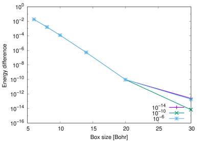
Figure 4: Energy difference in a CISD calculation from a simulation box of 40 Bohr with different IS thresholds of $10^{-14}$, $10^{-10}$ and $10^{-6}$. Due to the small energy differences at 20 and 30 Bohr compared to 40 Bohr these have been converged to $10^{-14}$ for all IS unlike the rest to $10^{-10}$. Like the exponential decay of the wave function an exponential decay of the energy contribution is seen irrespectively of the IS.

The difference at 30 Bohr does not lie on a straight line from the other points which is most likely due to the fact that we here are close to the convergence threshold of $10^{-14}$ and because the iterations in the SIAL are stopped based on the energy change from the previous iteration which does not decrease monotonically when the convergence threshold is very small.

V.2.2 Integral Screening

The number of two-electron integrals grows as $N_{orb}^{4}$ in Gaussian basis sets and these can therefore be problematic to store in memory or on disc if $N_{orb}$ is large. For large $N_{orb}$ the integrals will therefore have to be calculated on the fly when constructing the matrix elements in a traditional CI and the repeated calculation of integrals will become a bottleneck for very large basis sets.

The number of times an integral is calculated on the fly as a function of the simulation box for a regular CISD, an ISCISD and an ISCISD using the radial sparsity of the two-electron integrals are compared in Figure 5. The regular CI will recalculate both the trivially zero, in the FE-DVR basis, and numerically zero integrals for every matrix element while the ISCI will only recalculate these for every block of elements. If the number of electrons would scale with system size the difference between the regular CI and the ISCI would be significantly more pronounced due to the difference in scaling. Using the two-electron integral sparsity the scaling in the integral loop will be $N_{orb}^{2}$ and not $N_{orb}^{4}$ but even with the reduced scaling there is still a substantial numerical sparsity that can be exploited by rigorous IS.

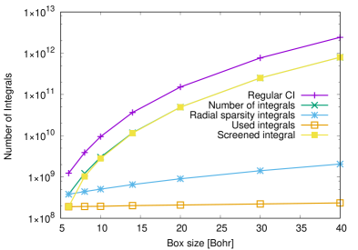
Figure 5: Number of integrals as a function of the simulation box size. Here the number of integrals are shown for a regular CISD calculation, an ISCISD and an ISCISD, where the radial sparsity of the FE-DVR basis set is used, are compared to the number of integrals used in the ISCI method and the number of screened integrals.

From Figure 6 it is seen that in the inner region half the integrals are screened away even though the construction of the orbitals in the SCF procedure destroys the sparsity of the FE-DVR basis in the inner region. Once the size of the box is increased the ratio of the screened integrals grows significantly and at 40 Bohrs less than $0.03$ percent of the integrals are used in the ISCI when the IS is $10^{-14}$. Even if the radial sparsity of the two-electron integrals is used only $11.5$ percent are used with a simulation box of 40 Bohrs.

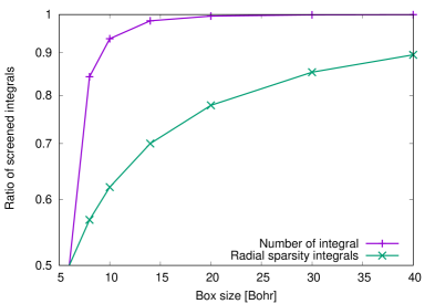
Figure 6: IS efficiency as a function of the size of the simulation box. The efficiency is here taken as the ratio between the number of screened integrals, and hence discharged integrals, and the total number of integrals both for an ISCISD and for an ISCISD using the two-electron integral sparsity of the FE-DVR basis.

For the vast majority of electronic structure calculations of atoms a simulation box of 40 Bohrs is not needed, however, once an external laser field is applied in order to study higher harmonic generation, photoionization and other processes where electrons move in the continuum a simulation box of 40 Bohrs is very small Larsson et al. (2016). For even larger simulation boxes the number of orbitals will typically be around $10^{3}$ to $10^{6}$ and here the benefits obtained by the IS procedure will be even more pronounced as can be seen from Figure 6. For such large basis sets it will no longer be possible to store all integrals and hence they will have to be calculated on the fly. Due to the numerous times an integral will have to be recalculated in a regular CI this becomes an insurmountable bottleneck and the regular CI is therefore not even able to solve the time-independent problem for small systems in the very large basis sets typically used in time-dependent simulations involving the continuum.

For large molecular systems we expect to see similar trends in the IS as a function of distance if local orbitals are used Høyvik et al. (2014, 2012). Here the screening efficiency will of course not be as rapid as seen in Figure 6 due to interactions within the molecule.

V.2.3 Floating point operations

As seen in Section V.2.2 the vast majority of the integrals can be screened away and since the ISCI only uses the integrals above the screening threshold in the $\sigma$-vector step this will result in a reduced scaling of the $\sigma$-vector step. In Figure 7 the number of floating point operations in the $\sigma$-vector step as a function of the size of the simulation box for a CISD, a CISD using the radial sparsity and an ISCISD calculation are compared. It is readily seen that the scaling of the ISCISD is lower than the CISD and also significantly lower than a CISD using the radial sparsity. Once the simulation box is extended to 40 Bohrs the regular CISD and the CISD using radial sparsity is using $10^{3}$ and $10$ times as many floating point operations as the ISCI, respectively. It is therefore obvious that for even larger simulation boxes just using the radial sparsity of the two-electron integrals in a CI calculation will not suffice.

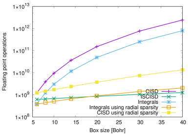
Figure 7: Floating point operations as a function of the size of the simulation box for a CISD, a CISD using radial sparsity and an ISCISD calculation along with the integral loops both with and without using the radial sparsity of the integrals.

The outer loop of the ISCI method is over all integrals and as can be seen in Figure 7 this loop will be the dominating step for the ISCI method. If the radial sparsity of the two-electron integrals is not used then the integral loop will only reduce the savings compared to the regular CI by around two thirds in this case. However, if the radial sparsity of the two-electron integrals is used, the integral loop will have a scaling of $N_{orb}^{2}$ and a significant reduction is observed. Despite this significant reduction in the scaling of the integral loop it is still more expensive than the $\sigma$-vector step in the ISCI approach when the size of the simulation box is increased.

The IS in the ISCI is directly translated into a screening of the floating point operation in the $\sigma$-vector step as can be seen by comparing Figures 6 and 8 since the floating point operations screening follows the IS closely. Here only $0.05$ percent of the floating points operations in the $\sigma$-vector step are carried out in the ISCISD compared to the CISD with a simulation box of 40 Bohrs and an IS threshold of $10^{-14}$. When the radial sparsity of the two-electron integrals is used, only $9.8$ percent of the $\sigma$-vector step have to be performed in the ISCI.

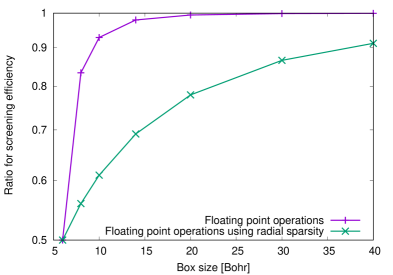
Figure 8: Floating point operations screening efficiency in the $\sigma$-vector step as a function of the size of the simulation box. The efficiency is here taken as the ratio between the floating point operations screened away in the ISCISD and the total floating point operations for the CISD and for a CISD using the two-electron integral sparsity of the FE-DVR basis.

The screening threshold has an impact on both the accuracy and efficiency of the floating point screening. In Figure 9 the floating point operations with different IS threshold are compared. Not surprisingly, the number of floating point operations in the $\sigma$-vector step is reduced when the IS threshold is increased. There is, however, no abrupt stop for integrals above a certain size depending on distance since there will always be integrals with large values within each FE and it is therefore only the long range interaction that is screened away when the size of the simulation box is increased.

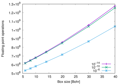
Figure 9: Comparison of the floating point operations for different IS thresholds as a function of the simulation box size.

These large integrals that reside locally in the FE-DVR basis set are essential in order to describe electron-electron interaction away from the atom or molecule once an external field is applied to the system. For electronic structure calculations the large integrals far away from the nuclei are only very weakly coupled to the system and mainly help to describe the tail of the wave function as seen from Figure 4. These integrals are also the reason why the tail of the wave function for the highest IS threshold of $10^{-6}$ also gives small energy contributions. Without any prior knowledge of the distance within the system these integrals will have to be included in the ISCI. If, however, the distance between orbitals in different GAS are known this can be used to perform additional IS which depends on distance. An additional distance dependent IS will give linear scaling in both the integral loop and the $\sigma$-vector step.

The reduced scaling in the $\sigma$-vector step in the ISCI is not restricted to CISD but goes for all order in the CI hierarchy as seen in Figure 10. When increasing the box size the curve for the floating point operations of the higher order ISCI will cross with a lower order curve of the regular CI due to the reduced scaling of all orders in the ISCI. At 14 Bohrs the floating point operations for the ISCISDTQ is similar to the regular CISDT despite the ISCISDTQ at this point has 968.765.625 coefficients and the CISDT 30.691.241 coefficients as seen from Table 1. Furthermore at 40 Bohrs the floating point operations for the regular CISD is more than three times that of the ISCISDT despite the ISCISDT having 287 times more coefficients than the regular CISD.

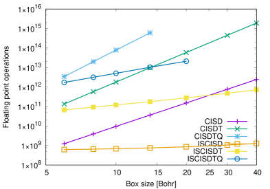
Figure 10: Comparison of the floating point operations in the $\sigma$-vector step between the CI and ISCI for different orders in the hierarchy.

V.2.4 Reduced scaling

The ISCI method gives reduced scaling, for spatially extended systems in local orbitals, for all orders of the CI hierarchy as can be seen in Figure 10. To obtain the scaling of the different orders of the ISCI method a simple fit of the floating point operations is performed. The fit is from the inner region and until 20 or 40 Bohrs to show that there is a reduction in the scaling. These fits are performed with an IS threshold of $10^{-14}$ and the energy is therefore not changed by this. Afterwards we analyse the gradual reduction of the scaling in the $\sigma$-vector step and show that this will become linear for sufficiently large systems. Finally a comparison of different IS thresholds is performed in order to show the interplay between the IS and the scaling.

In Figure 11 the exponent for the scaling along with a linear curve have been fitted to the floating point operations as a function of box size for the ISCISD. We see that the ISCISD, in this case, scales as $1.24\pm 0.01$, very close to linear scaling, when the curve is fitted from 6 to 40 Bohrs. With this low scaling for the ISCISD in the $\sigma$-vector step it is therefore also evident why the integral loop, which has a scaling of 2 when using the two-electron integral sparsity above a certain box size, becomes the dominant step.

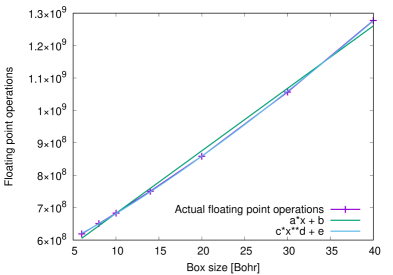
Figure 11: The exponent for the scaling and a linear curve have been fitted to the floating point operations as a function of box size for the ISCISD. The coefficients from the linear fit are $a=1.93\cdot 10^{7}$ and $b=4.90\cdot 10^{8}$ and for the exponent fit $c=7.48\cdot 10^{6}$, $d=1.24$ and $e=5.52\cdot 10^{8}$.

The low scaling of the ISCI continues to all orders of the CI hierarchy. The scaling going from the ISCISD to the ISCISDT, with the same fitting region, is only slightly increased to $1.48\pm 0.03$ as can be seen in Figure 12. Even though the scaling of the ISCISDT is lower than the scaling of the integral loop, even when using the two-electron integral sparsity, the prefactor will be dominant in the inner region but these curves will at some point cross when the size of the simulation box is increased sufficiently and then loop over the integrals will be the dominant one. For the ISCISDTQ the scaling is approximately quadratic, for a fit from 6 to 20 Bohrs, since the exponent is $1.98\pm 0.03$, see Figure 13, which is significantly lower than the usual scaling of CISDTQ which is $O^{4}V^{6}$.

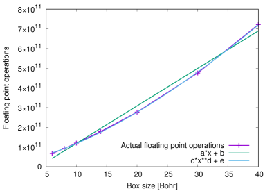
Figure 12: The exponent for the scaling and a linear curve have been fitted to the floating point operations as a function of box size for the ISCISDT. The coefficients from the linear fit are $a=1.90\cdot 10^{10}$ and $b=-7.18\cdot 10^{10}$ and for the exponent fit $c=2.97\cdot 10^{9}$, $d=1.48$ and $e=2.87\cdot 10^{10}$.

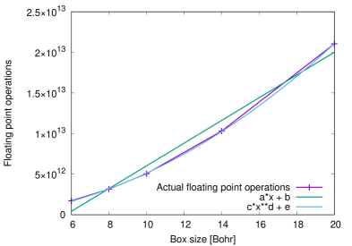
Figure 13: The exponent for the scaling and a linear curve have been fitted to the floating point operations as a function of box size for the ISCISDTQ. The coefficients from the linear fit are $a=1.40\cdot 10^{12}$ and $b=-7.98\cdot 10^{12}$ and for the exponent fit $c=5.68\cdot 10^{10}$, $d=1.98$ and $e=-2.93\cdot 10^{11}$.

The increase of the exponent with the excitation level in the ISCI is expectable since the scaling in CI grows as $O^{N}V^{N+2}$ and the decrease in the scaling in the ISCI is gradually reduced when the system size is increased. The reduction in scaling is accomplished without any prior knowledge about the structure of the CI-matrix, i.e., without using knowledge about the distance between orbitals, which can be used to screen large integrals which are centered far from the system. Such a distance dependent IS is often used to obtain linear scaling Sæbø and Pulay (1985); Hampel and Werner (1996); Ziółkowski et al. (2010); Schütz and Werner (2001); Flocke and Bartlett (2004); Pinski et al. (2015); Ettenhuber et al. (2010).

Usually when the system size is increased an increase in the floating point operations per FE in the $\sigma$-vector step, which depend on the scaling of the method, is expected. Due to the gradual reduction in scaling, until linear, the ISCI will instead approach a constant value.

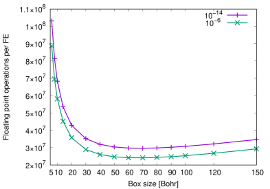
Figure 14: Floating point operations per FE for different box sizes with an IS cut-off of $10^{-14}$ and $10^{-6}$.

In Figure 14, a gradual reduction in the floating point operations per FE with system size can be seen. The gradual reduction is caused by the orbital rotation in the inner region, which destroys the sparsity of the FE-DVR basis, which makes the FE’s in the inner region significantly more expensive and the approach to a constant value is therefore not from below as normally seen. The floating point operations per FE therefore hits a minimum at around 70 Bohrs and then slightly increases again. With the lower IS threshold of $10^{-6}$ a reduction of 15-20 percent in the floating point operations in the $\sigma$-vector step is seen in this case.

V.2.5 Distribution of coefficients

The main problem in the ISCI is the number of coefficients. These are not screened since no prior knowledge about the CI-matrix is assumed. In Figure 15 the number of CI coefficients within a given range is plottet as a function of the size of the simulation box. The number of very small coefficients in Figure 15 is very dependent on the convergence threshold in the CI calculation. The convergence threshold for the energy in these calculations is $10^{-10}$. The plot in Figure 15 clearly shows that the larger the coefficients the less change in the number of these with distance. From around 14 Bohrs there is barely a change in the number of coefficients larger than $10^{-6}$ and at this distance the energy is converged to $5.2\times 10^{-7}$ which would be sufficient for most electronic structure calculations. For dynamics simulations the convergence in general have to be significantly stricter but for distances above 30-40 Bohrs it does appear possible to introduce sensible numerical approximations which do not effect the dynamics.

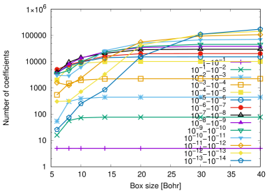
Figure 15: Number of coefficients in a given interval as a function of the size of the simulation box.

Here, approximation in the CI-vector similar to those done for the Hamiltonian in order to exploit the integral sparsity, can also be introduced which will significantly reduce the number of CI coefficients for large molecules and simulation boxes without compromising the accuracy of the calculations. By considering the sparsity of the CI-vector and a screening, the ISCI will be better able to handle higher excitations and large molecules in good basis sets simultaneously.

The long tail of small coefficients is almost completely independent of the IS threshold as can be seen from Figure 16 where the ratio between the number of CI coefficients below $10^{-14}$ and the total number of CI coefficients for different IS thresholds have been plotted. Since the number of small coefficients is practically the same for all IS thresholds we conclude that the long range contribution to the tail of the wave function comes from large integrals between local orbitals some distance away from the origin of the system.

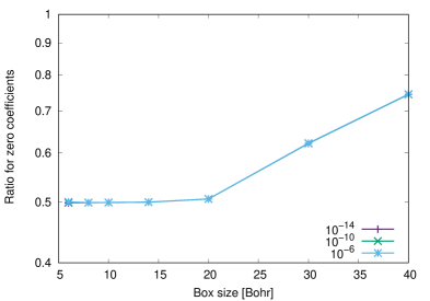
Figure 16: Ratio between the number of CI coefficients below $10^{-14}$ and the total number of CI coefficients for different IS thresholds of $10^{-6}$, $10^{-10}$ and $10^{-14}$.

The IS in the ISCI method can therefore still be numerically exact by letting the IS threshold be distance dependent. This would still give the tail for the wave function as seen in Figure 4 and at the same time allow for a reduction in the scaling to linear for any order in the ISCI and reduce the prefactor. The distance dependent IS can be combined with a screening of the CI coefficients this would make it possible to treat large systems using higher excitations.

VI Summary and prospects

We have presented a novel derivation of the well known CI equations which allows for an a priori integral screening (IS) of the integrals before the $\sigma$-vector step. The new method is dubbed the integral screened configuration interaction (ISCI) method. The IS appears naturally when the Hamiltonian is written in terms of normal- and spin-ordered and index restricted operators which is unlike the UGA Hamiltonian where the operators are written in terms of the generators of the unitary group.

By rewriting the Hamiltonian it is shown that the strings of second quantized operators in the $\sigma$-vector step are separable up to a sign. This separability allows for a construction of the $\sigma$-vector step where the outer loops are over the indices of the integrals in the Hamiltonian. Having the outer loops over the integrals allows for a very simple, efficient and rigorous a priori IS where only integrals above a predefined threshold are used in the $\sigma$-vector step. Such a procedure will automatically give a reduction in the scaling of the ISCI method for spatially extended systems in local basis sets. We here show that the scaling of the $\sigma$-vector step in the ISCI method gradually is reduced for all orders of the CI hierarchy when the system size grows until eventually a linear scaling is achieved.

Since the usual machinery from CI, such as the lexicographical scheme, does not appear to be directly applicable to the ISCI method we give a detailed description of the current way of solving these problems in the ISCI approach. Here we also show some of the 42 unique ways of contracting a non-relativistic Hamiltoian with the CI-vector and how each of these can be separately optimized. Furthermore we also show how the same code can be used to calculate density matrices.

A numerical example on Be is shown where the size of the simulation box is extended from 6 to 150 Bohrs and the scaling of the ISCI method is examined. We furthermore show that from a low IS threshold of $10^{-14}$ we can obtain a scaling for the ISCISD of $1.24\pm 0.01$, for the ISCISDT of $1.48\pm 0.03$ and finally for the ISCISDTQ of $1.98\pm 0.03$. We note that the scaling depends on the IS threshold so by increasing the IS threshold the scaling will be even further decreased. We also show that for sufficiently large simulation boxes the loop over the integrals, even when using the two-electron integral sparsity of the FE-DVR basis set, will be the dominant step for all orders of the ISCI method.

In the application part we discuss the effect of the IS for both electronic structure theory and for dynamics simulations in strong laser fields since the requirements here sometimes are different. We also show how the two-electron integral sparsity of the FE-DVR basis set can be exploited using the generalized-active-space (GAS) approach. Furthermore we lay out the path to linear scaling for all orders of the ISCI and discuss how to obtain distance dependent integral and coefficient screening in an efficient way that does not compromise the accuracy in neither electronic structure calculation nor in time-dependent simulations.

Currently the main aim of the method is accurate simulations of physical processes where one or more electrons move in the continuum for atoms and molecules in strong laser fields. Including both electron correlation and simulating electron processes involving the continuum is a major theoretical and numerical challenge and usually involves severe approximations in either the particle interaction, the description of the continuum, the initial and subsequent correlation level or combinations of these. With the ISCI method we aim for being able to treat up to two electrons in the continuum accurately. We also believe that the present type of IS would not only be of interest for time-dependent simulations of dynamics of electrons in the continuum but also suitable for electron structure theory since the electron-electron interaction at large distances is dominated by the local field. In electronic structure theory the rigorous IS will give a very good error control and in combination with the GAS will allow for low or linear scaling ISMRCI calculations which could serve as an alternative to the embedding schemes. The main problem with extending the method to very large systems is the lack of size-extensivity in truncated CI. In the near future we plan to interface the GASCI part with a quantum chemistry code which can provide local orbitals for large molecules to show the scaling properties of the ISCI for these kind of systems. Here we also plan to introduce the distance dependent integral and coefficient screening.

Appendix A The CAAB representation

The Creator Annihilator Alpha Beta (CAAB) representation was first introduced in the LUCIA code ols ; Olsen (2000) and has since been used in several other codes Sørensen et al. (2009, 2010); Sørensen and Olsen (2016); Sørensen et al. (2011). The CAAB operator in our implementation is similar to the one in LUCIA with the exception that we can vary the number of spin orbitals within the same GAS completely independent of each other. The CAAB operator is an abstract representation of a second quantized operator which can easily be manipulated on a computer and presents an extremely convenient way to setup the generalized active space (GAS). The representation of a CAAB operator with a GAS can be set in a matrix form with four rows, the creator $\alpha$, creator $\beta$, annihilator $\alpha$ and annihilator $\beta$, and NGAS column, where NGAS is the number of GAS. The entries in the matrix in the CAAB representation is the number second quantized operators in a given GAS.

As an example of the CAAB representation the $\hat{X}_{2,0,0}$ operator in two GAS is chosen. Here the first GAS will be the occupied space while the second will be the virtual space since we in this way will have a well-defined Fermi vacuum. The $\hat{X}_{2,0,0}$ operator in the CAAB representation, where the operator is called a type, is

$$CA\qquad 0\quad 1$$

$$CB\qquad 0\quad 1$$

$$AA\qquad 1\quad 0$$

$$AB\qquad 1\quad 0$$ (82)

where $CA$ stands for creation $\alpha$, $CB$ for creation $\beta$, $AA$ for annihilation $\alpha$ and $AB$ for annihilation $\beta$. In Eq. A it is seen that an electron with $\alpha$ and $\beta$ spin is excited from the occupied space to the virtual space by annihilation of an electron with $\alpha$ and $\beta$ spin in the occupied space and creation of an electron with $\alpha$ and $\beta$ spin in the virtual space. Splitting the virtual space into two, the $\hat{X}_{2,0,0}$ operator from Eq. A is split into four types

$$CA \qquad 0\quad 1\quad 0$$ (83)

$$CB \qquad 0\quad 1\quad 0$$

$$AA \qquad 1\quad 0\quad 0$$

$$AB \qquad 1\quad 0\quad 0$$

$$CA \qquad 0\quad 0\quad 1$$ (84)

$$CB \qquad 0\quad 1\quad 0$$

$$AA \qquad 1\quad 0\quad 0$$

$$AB \qquad 1\quad 0\quad 0$$

$$CA \qquad 0\quad 1\quad 0$$ (85)

$$CB \qquad 0\quad 0\quad 1$$

$$AA \qquad 1\quad 0\quad 0$$

$$AB \qquad 1\quad 0\quad 0$$

$$CA \qquad 0\quad 0\quad 1$$ (86)

$$CB \qquad 0\quad 0\quad 1$$

$$AA \qquad 1\quad 0\quad 0$$

$$AB \qquad 1\quad 0\quad 0$$

The splitting of the types in the CAAB representation is also visible in the $|\hat{X}_{2,0,0}\rangle\langle\hat{X}_{2,0,0}|\hat{H}|\hat{X}_{2,0,0}\rangle\langle\hat{X}_{2,0,0}|$ block when going from Figure 2 to Figure 3. In Figure 2 the matrix element $|\hat{X}_{2,0,0}\rangle\langle\hat{X}_{2,0,0}|\hat{H}|\hat{X}_{2,0,0}\rangle\langle\hat{X}_{2,0,0}|$ is a single block represented by the CAAB type in Eq. A while in Figure 3 $|\hat{X}_{2,0,0}\rangle\langle\hat{X}_{2,0,0}|\hat{H}|\hat{X}_{2,0,0}\rangle\langle\hat{X}_{2,0,0}|$ is split into four times four smaller blocks from the splitting of the $\hat{X}_{2,0,0}$ CAAB type into the four $\hat{X}_{2,0,0}$ CAAB types in Eqs. 83-86. Increasing the number of GAS will increase the number of blocks while at the same time reduce the size of the individual blocks which will help to give a good load balancing for a parallelization of the code since every block in the CI matrix is addressed individually. It is important to stress that using the CAAB representation of $\hat{X}_{2,0,0}$ in Eq. A or those in Eqs. 83-86 will give identical results and the only difference is how the algorithm performs the calculation.

For approximations with only a single electron in the continuum Bauch et al. (2014) the three GASs can be divided into occupied orbitals, unoccpied bound orbitals $(E<0)$ and continuum orbital $(E>0)$. Since only one electron should be in the continuum the $\hat{X}_{2,0,0}$ CAAB representation will then just consists of the types in Eqs. 83-85 since the type in Eq. 86 would place two electrons in the continuum. Since the continuum typically contains the vast majority of the orbitals removing the operator in Eq. 86 from the calculation will often reduce the computational effort by several magnitudes.

Connecting the CAAB representation of the Hamiltonian to the excitation and de-excitation operators in Eq. 28 can be done by a two-GAS setup where the occupied orbitals are in the first space and the unoccupied in the second. In this way all 8 terms from Eq. 28 can be distributed in the entries of the types

$$CA \qquad\hat{C}_{\alpha}^{dx}\quad\hat{C}_{\alpha}^{ex}$$ (87)

$$CB \qquad\hat{C}_{\beta}^{dx}\quad\hat{C}_{\beta}^{ex}$$

$$AA \qquad\hat{A}_{\alpha}^{ex}\quad\hat{A}_{\alpha}^{dx}$$

$$AB \qquad\hat{A}_{\beta}^{ex}\quad\hat{A}_{\beta}^{dx}$$

whereby any term in the Hamiltonian can be written. From the generic type in Eq. 87 any excitation or de-excitation term can easily be found, addressed and manipulated. The generalization of Eq. 87 to many GASs is simple as long as the occupied and virtual orbitals are in separate GASs and follow directly from the example of $\hat{X}_{2,0,0}$ above. Combining the index-restricted Hamiltonian in Eq. II.1 with the generic Hamiltonian type in Eq. 87 any term in the Hamiltonian can be written as shown in Eq. 28.

The manipulation of the types is the first step performed in any calculation where the non-zero blocks in the CI matrix are identified. Here we have two operations where the first is contraction and the second addition. In the $\sigma$-vector step in Eq. 9 all de-excitation terms in the Hamiltonian are contracted with the approximate eigenvector ${\mathbf{v}}$ while all the excitation terms in the Hamiltonian will add to ${\mathbf{v}}$. The result of the contraction and addition will give the linearly transformed approximate eigenvector ${\mathbf{\sigma}}$. In the CAAB representation of operators the application of

$$\hat{H}_{2,0,-2}^{2,1}\hat{v}_{3,0,-1}=\hat{\sigma}_{2,0,0}$$ (88)

in the $\sigma$-vector step is

$$CA \qquad 0\quad 0$$

$$\hat{H}_{2,0,-2}^{2,1}=\quad CB \qquad 1\quad 1$$ (89)

$$AA \qquad 0\quad 0$$

$$AB \qquad 0\quad 2$$

$$CA \qquad 0\quad 1$$

$$\hat{v}_{3,0,-1}=\quad CB \qquad 0\quad 2$$ (90)

$$AA \qquad 1\quad 0$$

$$AB \qquad 2\quad 0$$

$$CA \qquad 0\quad 1$$

$$\hat{\sigma}_{2,0,0}=\quad CB \qquad 0\quad 1$$ (91)

$$AA \qquad 1\quad 0$$

$$AB \qquad 1\quad 0$$

where $\hat{\sigma}_{2,0,0}$ results from the application of $\hat{H}_{2,0,-2}^{2,1}$ on $\hat{v}_{3,0,-1}$. The contraction of the $\hat{A}_{\beta}^{dx}$ term in $\hat{H}_{2,0,-2}^{2,1}$ with $\hat{v}_{3,0,-1}$ happens by subtracting the two in the $AB$ line in Eq. A with the two in the $CB$ line in Eq. A which are the two particle contractions. The hole contraction, which is the $\hat{C}_{\beta}^{dx}$ part of $\hat{H}_{2,0,-2}^{2,1}$, happens by subtraction of the first one in the $CB$ line in Eq. A with one of the two in the $AB$ line in Eq. A. The resulting CAAB operator for the Hamiltonian after the contraction is

$$CA \qquad 0\quad 0$$ (92)

$$CB \qquad 0\quad 1$$

$$AA \qquad 0\quad 0$$

$$AB \qquad 0\quad 0$$

and for $\hat{v}_{3,0,-1}$ is

$$CA \qquad 0\quad 1$$ (93)

$$CB \qquad 0\quad 0$$

$$AA \qquad 1\quad 0$$

$$AB \qquad 1\quad 0$$

where both now only contain excitation terms which are added to give $\hat{\sigma}_{2,0,0}$ in Eq. A. In this way all possible non-zero blocks in the CI matrix can quickly be found and tabulated. The algorithm can in this way be guided by which part of the $\sigma$-vector step should be calculated.

From these examples it is seen how a second quantized operator can be represented in the computer and how approximations easily can be introduced just by dividing the GAS appropriately and then eliminating the unwanted types. Furthermore the direct connection between the excitation and de-excitation operators in Eq. 28 and the types for the CAAB representation is shown. It is the types in the CAAB representation that is setup and manipulated in the first part of the algorithm in Section IV.3.1 and the types for a contraction is then passed down to the $\sigma$-vector step, shown in Section IV.3.2, where this is translated into one of the 42 loop structures and calculated.

References

- Kellner (1927a) G. W. Kellner, Z. Phys. 44, 91 (1927a).
- Kellner (1927b) G. W. Kellner, Z. Phys. 44, 110 (1927b).
- Hylleraas (1928) E. A. Hylleraas, Z. Phys. 48, 469 (1928).
- Shavitt (1998) I. Shavitt, Mol. Phys. 94, 3 (1998).
- Cremer (2013) D. Cremer, WIREs Comput. Mol. Sci. 3, 482 (2013).
- Møller and Plesset (1934) C. Møller and M. S. Plesset, Phys. Rev. 46, 618 (1934).
- F. Coester (1958) F. Coester, Nuc. Phys. 7, 421 (1958).
- F. Coester and H. Kümmel (1960) F. Coester and H. Kümmel, Nuc. Phys. 17, 477 (1960).
- Hohenberg and Kohn (1964) P. Hohenberg and W. Kohn, Phys. Rev. B 136, 864 (1964).
- Kohn and Sham (1965) W. Kohn and L. J. Sham, Phys. Rev. 140, 1133 (1965).
- Bartlett and Musial (2007) R. J. Bartlett and M. Musial, Rev. Mod. Phys. 79, 291 (2007).
- Lyakh et al. (2012) D. I. Lyakh, M. Musiał, V. F. Lotrich, and R. J. Bartlett, Chem. Rev. 112, 182 (2012).
- Miyagi and Madsen (2013) H. Miyagi and L. B. Madsen, Phys. Rev. A 87, 062511 (2013).
- Sato and Ishikawa (2013) T. Sato and K. L. Ishikawa, Phys. Rev. A 88, 023402 (2013).
- Miyagi and Madsen (2014) H. Miyagi and L. B. Madsen, Phys. Rev. A 89, 063416 (2014).
- Bauch et al. (2014) S. Bauch, L. K. Sørensen, and L. B. Madsen, Phys. Rev. A 90, 062508 (2014).
- Hochstuhl and Bonitz (2012) D. Hochstuhl and M. Bonitz, Phys. Rev. A 86, 053424 (2012).
- Hochstuhl et al. (2014) D. Hochstuhl, C. M. Hinz, and M. Bonitz, Eur. Phys. J. Special Topics 223, 177 (2014).
- Klamroth (2003) T. Klamroth, Phys. Rev. B 68, 245421 (2003).
- Krause et al. (2005) P. Krause, T. Klamroth, and P. Saalfrank, J. Chem. Phys. 123, 074105 (2005).
- Rohringer et al. (2006) N. Rohringer, A. Gordon, and R. Santra, Phys. Rev. A 74, 043420 (2006).
- Greenman et al. (2010) L. Greenman, P. J. Ho, S. Pabst, E. Kamarchik, D. A. Mazziotti, and R. Santra, Phys. Rev. A 82, 023406 (2010).
- Grimme and Waletzke (1999) S. Grimme and M. Waletzke, J. Chem. Phys. 111, 5645 (1999).
- Kleinschmidt et al. (2002) M. Kleinschmidt, J. Tatchen, and C. M. Marian, J. Comput. Chem. 23, 824 (2002).
- Chwee et al. (2008) T. S. Chwee, A. B. Szilva, R. Lindh, and E. A. Carter, J. Chem. Phys. 128, 224106 (2008).
- Chwee and Carter (2010) T. S. Chwee and E. A. Carter, J. Chem. Phys. 132, 074104 (2010).
- Anderson (1975) J. B. Anderson, J. Chem. Phys. 63, 1499 (1975).
- Lüchow and Anderson (2000) A. Lüchow and J. B. Anderson, Ann. Rev. Phys. Chem. 51, 501 (2000).
- Caballol and Malrieu (1992) R. Caballol and J.-P. Malrieu, Chem. Phys. Lett. 180, 543 (1992).
- Bunge (2006) C. F. Bunge, J. Chem. Phys. 125, 014107 (2006).
- Bunge and Carbó-Dorca (2006) C. F. Bunge and R. Carbó-Dorca, J. Chem. Phys. 125, 014108 (2006).
- Almora-Díaz (2014) C. X. Almora-Díaz, J. Chem. Phys. 140, 184302 (2014).
- Shephard et al. (2014a) R. Shephard, G. Gidofalvi, and S. R. Brozell, J. Chem. Phys. 141, 064105 (2014a).
- Shephard et al. (2014b) R. Shephard, G. Gidofalvi, and S. R. Brozell, J. Chem. Phys. 141, 064106 (2014b).
- Nakatsuji (2000) H. Nakatsuji, J. Chem. Phys. 113, 2949 (2000).
- Nakatsuji and Davidson (2001) H. Nakatsuji and E. R. Davidson, J. Chem. Phys. 115, 2000 (2001).
- Nakatsuji (2005) H. Nakatsuji, Phys. Rev. A 72, 062110 (2005).
- Sherrill and Schaefer III (1999) C. D. Sherrill and H. F. Schaefer III, Adv. Quant. Chem. 34, 143 (1999).
- Roos (1972) B. O. Roos, Chem. Phys. Lett. 15, 153 (1972).
- Paldus (1974) J. Paldus, J. Chem. Phys. 61, 5321 (1974).
- Shavitt (1977) I. Shavitt, Int. J. Quantum Chem.: Quantum Chem. Symp. 11, 131 (1977).
- Olsen et al. (1988) J. Olsen, B. O. Roos, P. Jørgensen, and H. J. Aa. Jensen, J. Chem. Phys. 89, 2185 (1988).
- Larsson et al. (2016) H. R. Larsson, S. Bauch, L. K. Sørensen, and M. Bonitz, Phys. Rev. A 93, 013426 (2016).
- Bauch et al. (2016) S. Bauch, H. R. Larsson, C. Hinz, and M. Bonitz, Phys. Rev. A 696, 012008 (2016).
- Chattopadhyay et al. (2015) S. Chattopadhyay, S. Bauch, and L. B. Madsen, Phys. Rev. A 92, 063423 (2015).
- Sørensen and Olsen (2016) L. K. Sørensen and J. Olsen, Mol. Phys. (2016), DOI: 10.1080/00268976.2016.1195926.
- Sørensen et al. (2011) L. K. Sørensen, J. Olsen, and T. Fleig, J. Chem. Phys. 134, 214102 (2011).
- Davidson (1975) E. R. Davidson, J. Comput. Phys. 17, 87 (1975).
- Lanczos (1950) C. Lanczos, J. Res. Natl. Bur. Stand. 45, 225 (1950).
- Helgaker et al. (2000) T. Helgaker, P. Jørgensen, and J. Olsen, Molecular Electronic-Structure Theory (John Wiley & Sons, Ltd, Chichester, 2000).
- Pulay (1983) P. Pulay, Chem. Phys. Lett. 100, 151 (1983).
- Sæbø and Pulay (1985) S. Sæbø and P. Pulay, Chem. Phys. Lett. 113, 13 (1985).
- Ziółkowski et al. (2010) M. Ziółkowski, B. Jansík, T. Kjærgaard, and P. Jørgensen, J. Chem. Phys. 133, 014107 (2010).
- Hampel and Werner (1996) C. Hampel and H. J. Werner, J. Chem. Phys. 104, 6286 (1996).
- Høyvik et al. (2014) I. Høyvik, K. Kristensen, T. Kjærgaard, and P. Jørgensen, Theoret. Chim. Acta 133, 1417 (2014).
- Høyvik et al. (2012) I. Høyvik, B. Jansík, and P. Jørgensen, J. Chem. Phys. 137, 224114 (2012).
- Jensen et al. (1996) H. J. Aa. Jensen, K. G. Dyall, T. Saue, and K. Fægri, J. Chem. Phys. 104, 4083 (1996).
- Duch (1985) W. Duch, Int. J. Quantum Chem.: Quantum Chem. Symp. 27, 59 (1985).
- Duch and Karwowski (1982) W. Duch and J. Karwowski, Int. J. Quantum Chem.: Quantum Chem. Symp. 22, 783 (1982).
- Wasilewski (1989) J. Wasilewski, Int. J. Quantum Chem.: Quantum Chem. Symp. 36, 503 (1989).
- Duch (1986) W. Duch, Grms or Graphical Representation of Model Spaces: Vol 1 Basics (Lecture Notes in Chemistry Vol. 42, Springer-Verlag, 1986).
- Sørensen (2016) L. K. Sørensen, (2016), unpublished.
- Sørensen (2010) L. K. Sørensen, General Order Coupled-Cluster in the 4-Component Framework, Dissertation, Mathematisch-Naturwissenschaftliche Fakultät, Heinrich-Heine-Universität Düsseldorf (2010), http://www.theochem.hhu.de/fileadmin/redaktion/Fakultaeten/Mathematisch-Naturwissenschaftliche_Fakultaet/Chemie/Theo_Chem/Abschlussarbeiten/sorensen.lasse.diss.pdf.
- (64) DIRAC, a relativistic ab initio electronic structure program, Release DIRAC14 (2014), written by T. Saue, L. Visscher, H. J. Aa. Jensen, and R. Bast. with contributions from V. Bakken, K. G. Dyall, S. Dubillard, U. Ekström, E. Eliav, T. Enevoldsen, E. Faßhauer, T. Fleig, O. Fossgaard, A. S. P. Gomes, T. Helgaker, J. K. Lærdahl, Y. S. Lee, J. Henriksson, M. Iliaš, Ch. R. Jacob, S. Knecht, S. Komorovský, O. Kullie, C. V. Larsen, H. S. Nataraj, P. Norman, G. Olejniczak, J. Olsen, Y. C. Park, J. K. Pedersen, M. Pernpointner, R. di Remigio, K. Ruud, P. Sałek, B. Schimmelpfennig, J. Sikkema, A. J. Thorvaldsen, J. Thyssen, J. van Stralen, S. Villaume, O. Visser, T. Winther, and S. Yamamoto (see http://www.diracprogram.org).
- Rescigno and McCurdy (2000) T. Rescigno and C. McCurdy, Phys. Rev. A 62, 032706 (2000).
- Park and Light (1986) T. J. Park and J. C. Light, J. Chem. Phys. 85, 5870 (1986).
- Beck et al. (2000) M. H. Beck, A. Jäckle, G. Worth, and H.-D. Meyer, Phys. Rev. 324, 1 (2000).
- Schütz and Werner (2001) M. Schütz and H. J. Werner, J. Chem. Phys. 114, 661 (2001).
- Flocke and Bartlett (2004) N. Flocke and R. J. Bartlett, J. Chem. Phys. 121, 10935 (2004).
- Pinski et al. (2015) P. Pinski, C. Riplinger, E. F. Valeev, and F. Neese, J. Chem. Phys. 143, 034108 (2015).
- Ettenhuber et al. (2010) P. Ettenhuber, P. Baudin, T. Kjærgaard, P. Jørgensen, and K. Kristensen, J. Chem. Phys. 133, 014107 (2010).
- (72) Program LUCIA, a general CI code written by J Olsen, University of Aarhus, with contributions from H. Larsen and M. P. Fülscher.
- Olsen (2000) J. Olsen, J. Chem. Phys. 113, 7140 (2000).
- Sørensen et al. (2009) L. K. Sørensen, T. Fleig, and J. Olsen, J. Phys. B 42, 165102 (2009).
- Sørensen et al. (2010) L. K. Sørensen, T. Fleig, and J. Olsen, Z. Phys. Chem. 224, 671 (2010).