First passage time and stochastic resonance of excitable systems

Abstract

We study noise induced thermally activated barrier crossing of a Brownian particle that hops in a periodic ratchet potential where the ratchet potential is coupled with a spatially uniform temperature. The viscous friction $\gamma$ is considered to decrease exponentially when the temperature $T$ of the medium increases ($\gamma=Be^{-AT}$) as proposed originally by Reynolds am10 . The results obtained in this work show that the mean first passage time of the particle is considerably lower when the viscous friction is temperature dependent than that of the case where the viscous friction is temperature independent. Using exact analytic solutions and via numerical simulations not only we explore the dependence for the mean first passage time of a single particle but also we study the dependence for the first arrival time of one particle out of many particles. Our result exhibits that the first arrival time decreases as the number of particles increases. We then explore the thermally activated barrier crossing rate of the system in the presence of time varying signal. In this case, the interplay between noise and sinusoidal driving force in the bistable system may lead the system into stochastic resonance provided that the random tracks are adjusted in an optimal way to the recurring external force. The dependence of signal to noise ratio $SNR$ as well as the power amplification ($\eta$) on model parameters is explored. $\eta$ as well as SNR depicts a pronounced peak at a particular noise strength $T$. The magnitude of $\eta$ is higher for temperature dependent $\gamma$ case. In the presence of $N$ particles, $\eta$ is considerably amplified as $N$ steps up showing the the weak periodic signal plays a vital role in controlling the noise induced dynamics of excitable systems.

I Introduction

Studying the mean first passage time (MFPT) of various physical problems is vital and has diverse applications in many disciplinary fields such as science and engineering. In most cases, the MFPT is usually defined as the amount of time that a given particle takes to surmount a certain threshold where the threshold can be specified as a certain boundary, potential barrier and specified state. Particularly if one considers a Brownian particle moving in a viscous medium, assisted by the thermal background kicks, the particle presumably crosses the potential barrier. The magnitude of its MFPT relies not only on the system parameters, such as the potential barrier height, but also it depends on the initial and boundary conditions. Understanding of such noise induced thermally activated barrier crossing problem is vital to get a better understanding of most biological problems am1 ; am2 ; am3 ; am4 ; am5 ; am6 ; am7 ; am8 . In the past, considering temperature independent viscous friction, the dependence of the mean first passage time (equivalently the escape rate) on model parameters has been explored for various model systems, see for example the work am8 ; am9 ; am24 . However experiment shows that the viscous friction $\gamma$ is indeed temperature dependent and it decreases as temperature increases. In this work we discuss the role of temperature on the viscous friction as well as on the MFPT by taking a viscous friction $\gamma$ that decreases exponentially when the temperature $T$ of the medium increases ($\gamma=Be^{-AT}$) as proposed originally by Reynolds am10 . It is shown that the MFPT is smaller in magnitude when $\gamma$ is temperature dependent than when it is temperature independent. This is plausible since the diffusion constant $D=T/\gamma\propto k_{B}Te^{AT}$ is valid when the viscous friction considered to be temperature dependent showing that the effect of temperature on the particle mobility is twofold. First, it directly assists the particle to surmount the potential barrier. In other words, the particle jumps the potential barrier at the expenses of the thermal kicks. Second, when temperature increases, the viscous friction gets attenuated and as a result the diffusibility of the particle increases.

The first passage time problem has also been extensively studied in many excitable systems such as chemical reaction, neural system and cardiac system am111 ; am11 ; am12 . Particularly in cardiac system, the intra-cellular calcium dynamics is responsible for a number of trigged arrhythmias am12 . As discussed in our previous work am12 , the abnormal calcium release at a single microdomain level can be studied via master equation, where the corresponding Fokker-Planck equation can be written with an effective bistable potential. The MFPT for a single Brownian particle to cross the effective potential then corresponds to the time it takes for $n$ channels to open at a single microdomain level. Thus, although in the present paper we consider a simplified ratchet potential, our study gives us a clue regarding the dynamics of calcium ions in the cardiac system. Moreover membrane depolarization occurs if the simulations happen on tissue level when $N$ microdomains interact. The First passage time for one of these $N$ microdomains to fire for the first time can be found by calculating the MFPT that one particle takes out of $N$ particle to cross the potential barrier.

Exposing excitable systems to time varying periodic forces may result in an intriguing dynamics where in this case the coordination of the noise with time varying force leads to the phenomenon of stochastic resonance (SR) am13 ; am14 provided that the noise induced hopping events synchronize with the signal. The phenomenon of stochastic resonance has obtained considerable interests because of its significant practical applications in a wide range of fields. SR depicts that systems enhance their performance as long as the thermal background noise is synchronized with time varying periodic signal. Since the innovative work of Benzi et. al. am13 , the idea of stochastic resonance has been broadened and implemented to many model systems am15 ; am16 ; am17 ; am18 ; am19 ; am20 ; am21 ; am22 ; am23 . Recently the occurrence of stochastic resonance for a Brownian particle as well as for extended system such as polymer has been reported by us am24 ; am25 . Our analysis revealed that, due to the flexibility that can enhance crossing rate and change in chain conformations at the barrier, the power amplification exhibits an optimal value at optimal chain lengths and elastic constants as well as at optimal noise strengths. However most of these studies considered a viscous friction which is temperature independent. In this work, considering temperature dependent viscous friction, we study how the power amplification behaves as one varies the model parameters. We first explore the stochastic resonance of a single particle and we then study the SR for many particle system by considering both temperature dependent and independent viscous friction cases.

The aim of this paper is to explore the crossing rate and stochastic resonance of a single as well as many Brownian particles in a piecewise linear bistable potential by considering both temperature dependent and independent viscous friction cases. Although a generic model system is considered, the present study helps to understand the dynamics of excitable systems and it is also vital for basic understanding of statistical physics. The MFPT at single particle level is extensively studied in the past see for example the work am9 . However, the role of temperature on viscosity as well as on MFPT has not been studied in detail and this will be the subject of the present paper. Particularly, in the presence of time varying signal, we study how the background temperature affects the viscosity as well as the signal to noise ratio $SNR$ and spectral density$\eta$. On the other hand, the first passage time statistics at ensemble ($N$ particles) level has been explored in many studies am11 ; am12 . However, to best of our knowledge, the role of time-varying signal as well as the role of temperature on $SNR$ and $\eta$ has not been studied in detail at the ensemble level. In this work, via numerical simulations and using the exact analytic results, we study stochastic resonance of $N$ particles.

To give you a brief outline, in this work first we study the MFPT of a single particle both for temperature dependent and independent viscous friction cases. The exact analytic results as well as the simulation results depict that the MFPT is considerably smaller when $\gamma$ is temperature dependent. In both cases the escape rate increases as the noise strength increases and decreases as the potential barrier increases. We then extend our study for $N$ particle systems. The First passage time for one of the $N$ particles to fire for the first time $T_{N}$ can be found both analytically (at least in the high barrier limit) and via numerical simulation for a bistable system. It is found that $T_{N}$ is considerably smaller when the viscous friction is temperature dependent. For both cases, $T_{N}$ decreases as the noise strength increases and as the potential barrier steps down. In high barrier limit, $T_{N}=T_{s}/N$ where $T_{s}$ is the MFPT for a single particle. In general as the number of particles $N$ increases, $T_{N}$ decreases.

We then study our model system in the presence of time varying signal. In this case the interplay between noise and sinusoidal driving force in the bistable system may lead the system into stochastic resonance. Analytically and via numerical simulations, we study how the signal to noise ratio (SNR) and power amplification ($\eta$) behave as a function of the model parameters. $\eta$ as well as SNR depicts a pronounced peak at particular noise strength $T$. The magnitude of $\eta$ is higher for temperature dependent $\gamma$ case. In the presence of many particles $N$, $\eta$ is considerably amplified as $N$ steps up, showing that the weak periodic signal plays a vital role in controlling the noise induced dynamics of excitable systems.

The rest of the paper is organized as follows. In section II, we present the model. In section III, by considering both temperature dependent and independent viscous friction cases, we explore the dependence for MFPT on model parameters for a single as well as many particle systems. The role of sinusoidal driving force on enhancing the mobility of the particle is studied in IV. Section V deals with Summary and Conclusion.

II The model

Let us consider a Brownian particle that walks in a piecewise linear potential with an external load $U(x)$, where the ratchet potential $U(x)$ is given by

$$U(x)=\left\{\begin{array}[]{ll}U_{0}\left({~{}x\over L_{0}}+1\right),&\text{if}~{}~{}~{}-L_{0}\leq x\leq{0};\\ U_{0}\left(-{x\over L_{0}}+1\right),&\text{if}~{}~{}~{}{0}\leq x\leq L_{0}.\end{array}\right.$$ (1)

Here $U_{0}$ and $2L_{0}$ denote the barrier height and the width of the ratchet potential, respectively. The potential exhibits its maximum value $U_{0}$ at $x={0}$ and its minima at $x=-L_{0}$ and $x=L_{0}$. The ratchet potential is coupled with a uniform temperature $T$ as shown in Fig. 1.

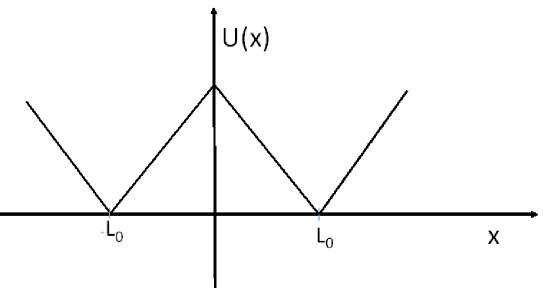
Figure 1: Schematic diagram for a Brownian particle in a piecewise linear potential. Due to the thermal background kicks, the particle ultimately surmounts the potential barrier.

For a Brownian particle that is arranged to undergo a random walk in a highly viscous medium, the dynamics of the particle is governed by Langevin equation am1 . The general stochastic Langevin equation, which is derived in the pioneering work of Petter Hänggi am2 , can be written as

$$\gamma{{dx}\over{dt}}=-\partial_{x}U-{(1-\epsilon)\gamma^{-1}}{\partial}_{x}(\gamma T)+\sqrt{2k_{B}\gamma T}\xi(t)$$ (2)

where $\gamma=\gamma(x)$ is the viscous friction, and $k_{B}$ is the Boltzmann’s constant am3 . The Itó and Stratonovich interpretations correspond to the case where $\epsilon=1$ and $\epsilon=1/2$, respectively while the case $\epsilon=0$ is known as the Hänggi a post-point or transform-form interpretation. At this point we want to stress that since we consider a uniform temperature profile, the expressions for thermodynamic quantities do not depend on the type of interpretation we use which implies the term ${(1-\epsilon)\over\gamma(x)}{\partial\over\partial x}(\gamma(x)T(x))$ can be omitted. Here after we adapt the Langevin equation

$$\gamma{dx\over dt} = -{\partial}_{x}U(x)+\sqrt{2k_{B}\gamma(x)T}\xi(t).$$ (3)

The viscous friction has an exponential temperature dependence

$$\gamma =Be^{-AT}, \text{if}~{}~{}~{}-L_{0}\leq x\leq{L_{0}}.$$ (4)

where $A$ and $B$ are constants. The random noise $\xi(t)$ is assumed to be Gaussian white noise satisfying the relations $\left\langle\xi(t)\right\rangle=0$ and $\left\langle\xi(t)\xi(t^{\prime})\right\rangle=\delta(t-t^{\prime})$ where $k_{B}$ and $B$ are considered to be unity.

In the high friction limit, the dynamics of the Brownian particle is governed by

$${\partial P(x,t)\over\partial t}={\partial\over\partial x}\left[{U^{\prime}(x)\over\gamma}P(x,t)+{\partial\over\partial x}\left({T\over\gamma}P(x,t)\right)\right]$$ (5)

where $P(x,t)$ is the probability density of finding the particle at position $x$ and time $t$. Here $U^{\prime}(x)={d\over dx}U$. At stationary state $J(x)=-\left[{U^{\prime}(x)\over\gamma}P_{s}(x)+{\partial\over\partial x}\left({T\over{\gamma}}P_{s}(x)\right)\right]$.

The diffusion constant $D={{k_{B}T}\over{\gamma}}=k_{B}Te^{AT}$ is valid when viscous friction to be temperature dependent showing that the effect of temperature on the particles’ mobility is twofold. First, it directly assists the particles to surmount the potential barrier; i. e. particles jump the potential barrier at the expenses of the thermal kicks. Second, when temperature increases, the viscous friction gets attenuated and as a result the diffusibility of the particle increases. Various experimental studies also showed that the viscosity of the medium tends to decrease as the temperature of the medium increases. This is because increasing the temperature steps up the speed of the molecules, and this in turn creates a reduction in the interaction time between neighboring molecules. As a result, the intermolecular force between the molecules decreases and hence the magnitude of the viscous friction decreases. Next we look at the dependence of the first passage time on the model parameters.

Hereafter, all the figures are plotted using the following dimensionless parameters: temperature ${\bar{T}}(x)=T(x)/T_{c}$, barrier height ${\bar{U}_{0}}=U_{0}/T_{c}$ and length ${\bar{x}}=x/L_{0}$. Moreover, all equations will be expressed in terms of the dimensionless parameters and for brevity we drop all the bars hereafter.

III The Mean first passage time of a single and many non-interacting particles

III.1 Mean first passage time for a single Brownian particle

We consider a single Brownian particle which is initially placed on the local minimum of a linear bistable potential as shown in Fig. 1. Due to the thermal background kicks, the particle presumably crosses the potential barrier. The magnitude of the crossing rate of the particle strictly relies on the barrier height and noise strength as well as on the length of the ratchet potential.

The mean first passage time $T_{s}$ for Brownian particle that walks on the ratchet potential can be found via

$$T_{s}=\int_{-L_{0}}^{L_{0}}dxe^{U(x)\over T}\int_{-L_{0}}^{x}dz{e^{-U(z)\over T}\over h}$$ (6)

where $h={T\over\gamma}$ am26 . If one imposes a reflecting boundary condition at $x=-L_{0}$ and absorbing boundary condition at $x=L_{0}$, Eq. (6) converges to

$$T_{s}=T_{1}+T_{2}$$ (7)

where

$$T_{1} = \int_{-L_{0}}^{0}dxe^{U^{1}(x)\over T}\int_{-L_{0}}^{x}dz{e^{-U^{1}(z)\over T}\over h}$$ (8)

$$= {L_{0}^{2}[T(-1+e^{U_{0}\over T})-U_{0}]\over U_{0}^{2}}e^{-AT}$$

and

$$T_{2} = \int_{0}^{L_{0}}dxe^{U^{2}(x)\over T}\int_{-L_{0}}^{0}dz{e^{-U^{1}(x)\over T}\over h}+$$ (9)

$$\int_{0}^{L_{0}}dxe^{U^{2}(x)\over T}\int_{0}^{L_{0}}dz{e^{-U^{2}(z)\over T}\over h}$$

$$= {{L_{0}^{2}[U_{0}+T(-3+3\cosh[{U_{0}\over T}]-\sinh[{U_{0}\over T}])]}\over{U_{0}^{2}}}e^{-AT}$$

where $U^{1}(x)=U_{0}\left({x\over L_{0}}+1\right)$ and $U^{2}(x)=U_{0}\left({{-x}\over L_{0}}+1\right)$. After some algebra we find

$$T_{s}={4TL_{0}^{2}e^{-AT}\left(-1+\cosh[{U_{0}\over T}]\right)\over U_{0}^{2}}.$$ (10)

Equation (10) is an exact analytic expression and its validity is justified using numerical simulations. In high barrier limit $U_{0}\to\infty$, $T_{s}$ approaches

$$T_{s}={2TL_{0}^{2}e^{-AT}e^{{U_{0}\over T}}\over U_{0}^{2}}.$$ (11)

For temperature independent viscous friction ($A=0$), one retrieves

$$T_{s}={4TL_{0}^{2}\left(-1+\cosh[{U_{0}\over T}]\right)\over U_{0}^{2}}.$$ (12)

In high barrier limit $U_{0}\to\infty$, $T_{s}$ approaches

$$T_{s}={2TL_{0}^{2}e^{{U_{0}\over T}}\over U_{0}^{2}}.$$ (13)

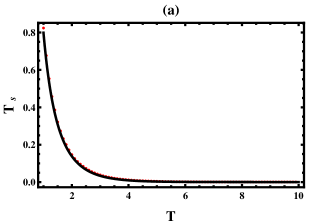
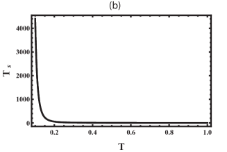
Figure 2: (Color online)(a) The mean first passage time $T_{s}$ as a function of $T$ for the parameter values of $A=1.0$, $U_{0}=1.0$ and $L_{0}=1.0$. (b) The mean first passage time $T_{s}$ as a function of $T$ for the parameter values of $A=1.0$, $U_{0}=2.0$ and $L_{0}=1.0$. In the figures the red dotted line is evaluated numerically while the solid line is plotted using the exact analytic expression (Eq. 10).

The exact analytic results are justified via numerical simulations by integrating the Langevin equation (3) (employing Brownian dynamics simulation). In the simulation, a Brownian particle is initially situated in one of the potential wells. Then the trajectories for the particle is simulated by considering different time steps $\Delta t$ and time length $t_{max}$. In order to ensure the numerical accuracy, up to $10^{8}$ ensemble averages have been obtained

Via numerical simulations as well as using the exact analytic expression, we first plot the MFPT for temperature dependent viscous friction case ($A=1$) as shown in Figs. 2a and 2b. In the figure the red dotted line is evaluated numerically while the solid line is plotted using the exact analytic expression (Eq. 10). The figure depicts that $T_{s}$ monotonically decreases as the background temperature increases. In the small regime of $T$ (See Fig. 2b), $T_{s}$ decays exponentially. Exploiting Eq. (10), one can see that the MFPT is considerably higher when the viscous friction is temperature dependent ($A=1$) than constant $\gamma$ case ($A=0$). As the barrier height increases, $T_{s}$ increases.

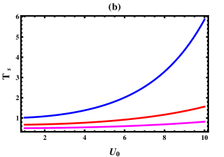
Figure 3: (Color online)(a) The mean first passage time $T_{s}$ as a function of $U_{0}$ for fixed values of $A=1.0$ (variable $\gamma$ case), $T=2.0$, $T=3.0$, $T=4.0$ and $L_{0}=1.0$ from top to bottom, respectively. (b) The mean first passage time $T_{s}$ as a function of $U_{0}$ for the parameter values of $A=0$ (constant $\gamma$ case), $T=2.0$, $T=3.0$, $T=4.0$ and $L_{0}=1.0$ from top to bottom, respectively.

In Figs. 3a and 3b, the mean first passage time $T_{s}$ is plotted as a function of $U_{0}$ for the parameter values of $T=2.0$, $T=3.0$, $T=4.0$ and $L_{0}=1.0$ from top to bottom, respectively. Fig. 3a represents the constant $\gamma$ while Fig. 3b shows the temperature dependent $\gamma$ cases. The figure depicts that $T_{s}$ decreases monotonically as the background temperature increases. The same figure depicts also that $T_{s}$ increases as the barrier height $U_{0}$ steps up.

It is important to note that most of the previous studies of thermally activated barrier crossing rate considered only temperature invariance viscous friction case. In reality, it is well know that the mean first passage time of a Brownian particle tends to depend on the intensity of the background temperature. However in liquid or glassy medium, the viscosity tends to decrease when the intensity of the background temperature increases. This is because an increase in temperature of the medium brings more agitation to the molecules in the medium, and hence increases their speed. This speedy motion of the molecules creates a reduction in interaction time between neighboring molecules. In turn, at macroscopic level, there will be a reduction in the intermolecular force. Consequently, as the temperature of the viscous medium decreases, the viscous friction in the medium decreases which implies that the mobility of the particle considerably increases (MFPT decreases) when the temperature of the medium increases. The main message here is that the effect of temperature on the viscous friction is significantly high and cannot be avoided unlike the previous studies.

III.2 Mean first passage time of many Brownian particles

Let us now consider the First passage time for one of the $N$ particles to cross the potential barrier for the first time. Studying such physical problem is vital and has been extensively studied in many excitable model systems such as cardiac systems. Most of these studies have considered temperature independent viscous friction. In this section we explore further how the temperature of the medium affects the viscosity as well as the the first passage time.

First let us numerically evaluate the first passage time distribution for a single and many particle systems. This gives us a qualitative clue on how the first passage time behaves because the first passage time is given by $T=\int_{0}^{t}t^{\prime}P_{i}(t^{\prime})dt^{\prime}$ where $P_{i}(t^{\prime})$ is the first time distribution of the $i^{th}$ particle. In Fig. 4, the first passage time distribution of a single particle $P_{i}(t)$ as a function of $t$ is depicted for $U_{0}=1.0$ and $L_{0}=1.0$. In the figure the $A=0.0$ (temperature independent $\gamma$) and $A=1.0$ (temperature dependent $\gamma$) cases are shown in the red and green lines respectively. Compared to the constant $\gamma$ case, the figure depicts that the peak of the first time distribution gets higher, and its location shifts to the left when the viscous friction is temperature dependent. On the other hand, the plot for the first time distribution $P_{N}(t^{\prime})$ for one of the $N$ particles to fire is shown in Fig. 5a (constant viscous friction case) and Fig. 5b (temperature dependent viscous friction case). As $N$ increases, the peak of the first passage time distribution decreases revealing that the firing time for one particle (out of the $N$ particles) decreases as $N$ increases.

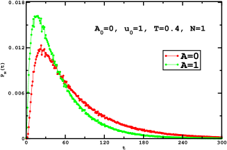
Figure 4: (Color online) The first passage time distribution $P_{i}(t)$ as a function of $t$ for $N=1$ and for the parameter values of $U_{0}=1.0$ and $L_{0}=1.0$. The plots for $A=0$ and $A=1.0$ cases are shown in the red and green lines, respectively.

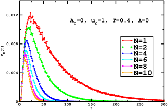
(a)

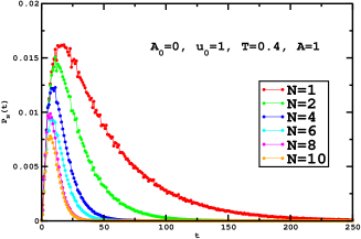
(b)

Figure 5: (Color online) The first passage time distribution $P_{N}(t)$ as a function of $t$ for different values of $N$. We use parameter values of $U_{0}=1.0$ and $L_{0}=1.0$. Figures (a) and (b) show the distributions for the cases $A=0$ and $A=1$, respectively.

In the high barrier limit, the first passage time distribution $P_{i}(t)$ is computable as discussed in many litterateurs. To begin with, the Fourier transform of first passage time distribution is the characteristic function $\Phi(k,y)$ is given by

$$\Phi(k,y)=\left\langle exp(ikT)\right\rangle=\sum_{n=0}^{\infty}{(ik)^{n}\over n!}T_{n}(y).$$ (14)

Let us define an integral Kernel $K(y,z^{\prime})$ as

$$K(y,z^{\prime})=\int_{y}^{0}dx{1\over h(x){\mathscr{P}}_{s}(x)}\int_{-\infty}^{x}dz{\mathscr{P}}_{s}(z)\delta(z-z^{\prime}).$$ (15)

Here ${\mathscr{P}}_{s}(x)$ denotes the equilibrium probability distribution. Then the characteristic function $\Phi(k,y)$ is derived as

$$\Phi(k,y) = 1+ik\int_{\infty}^{0}dz^{\prime}K(y,z^{\prime})+$$ (16)

$$(ik)^{2}\int_{\infty}^{0}dz_{1}\int_{\infty}^{0}dz_{2}K(y,z_{1})K(z_{1},z_{2})+\cdots$$

In the high barrier limit, one gets

$$\Phi(k,y)=\sum_{n=0}^{\infty}{(ikT_{s})^{n}}={i\over i+kT_{s}}.$$ (17)

The inverse Fourier transform of $\Phi(k,y)$ is the first passage distribution $P_{i}(t)$, and after some algebra we get

$$P_{i}(t)={e^{{-t\over T_{s}}}\over T_{s}}$$ (18)

where $T_{s}$ is the MFPT for a single particle.

Once we compute $P_{i}(t)$, the first passage time distribution for one particle to cross the barrier out a given $N$ particles can be evaluated using

$$P_{N}(t)=\sum_{i-1}^{N}P_{i}(t)\prod_{j\neq i}(1-k_{j}(t))$$ (19)

where

$$k_{j}(t)=\int_{0}^{t}dt^{\prime}P_{j}(t^{\prime}).$$ (20)

After some algebra we find

$$P_{N}(t)={e^{{-t\over T_{N}}}\over T_{N}}.$$ (21)

The first arrival time $T_{N}$, i. e. the time for one of the particles first to cross the potential barrier, is calculated via

$$T_{N}=\int_{0}^{t}t^{\prime}P_{N}(t^{\prime})dt^{\prime}.$$ (22)

For such a case, Eq. (22) reduces to

$$T_{N}={T_{s}\over N}={{2TL_{0}^{2}e^{-AT}e^{U_{0}\over T}}\over{NU_{0}^{2}}}.$$ (23)

Exploiting Eq. (23) one can see that as the temperature increases, $T_{N}$ decreases exponentially while as the barrier height $U_{0}$ increases, the MFPT decreases. We also note that as the number of particles increases $T_{N}$ decreases.

The mean first passage time $T_{N}$ as a function of $T$ is depicted in Fig. 6a for the parameter values of $U_{0}=2.0$, $N=1.0$, $N=2$, $N=3.0$ and $L_{0}=1.0$ from top to bottom, respectively. The viscous friction is considered to be temperature dependent. In Fig. 6b, the mean first passage time $T_{N}$ as a function of $T$ is plotted for the parameter values of $U_{0}=2.0$, $N=1.0$, $N=2$, $N=3.0$ and $L_{0}=1.0$ from top to bottom, respectively considering temperature independent viscous friction. As depicted in the figures, $T_{N}$ decreases as the noise strength increases and when the number of particle increases.

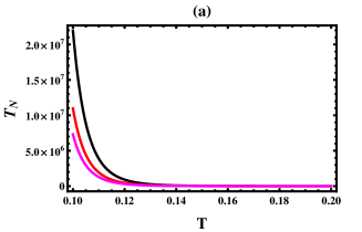
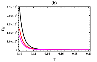
Figure 6: (Color online)(a) The mean first passage time $T_{N}$ as a function of $T$ for the parameter values of $U_{0}=2.0$, $N=1.0$, $N=2$, $N=3.0$ and $L_{0}=1.0$ from top to bottom, respectively for a variable $\gamma$ case. (b) The mean first passage time $T_{N}$ as a function of $T$ for the parameter values of $U_{0}=2.0$, $N=1.0$, $N=2$, $N=3.0$ and $L_{0}=1.0$ from top to bottom, respectively for a constant $\gamma$ case.

IV Stochastic resonance for a single and many non-interacting particles

In the presence of time varying signal, the interplay between noise and sinusoidal driving force in the bistable system may lead the system into stochastic resonance, provided that the random tracks are adjusted in an optimal way to the recurring external force. Various studies have used different quantities to study the SR of systems that are driven by a time varying signal. These includes signal to noise ration (SNR), spectral power amplification ($\eta$), the mean amplitude, as well as the residence-time destitution, which all exhibit a pronounced peak at a certain noise strength as long as the noise induced hopping events are synchronized with the signal. In this section we study the dependence SNR and $\eta$ on the model parameters by considering a continuous diffusion dynamics and provide a new way to look at the SR on the system.

In the presence of a time varying periodic signal $A_{0}\cos(\Omega t)$, the Langevin equation that governs the dynamics of the system is given by

$$\gamma{dx\over dt} = -{\partial U\over\partial x}+A_{0}\cos(\Omega t)+\sqrt{2k_{B}\gamma T}\xi(t).$$ (24)

where $A_{0}$ and $\Omega$ are the amplitude and angular frequency of the external signal respectively. Eq. 24 is numerically simulated for both small and large barrier heights. The first passage time distribution $P_{i}(t)$ shows the resonance profile at the right frequency match.

Before exploring how the signal to noise ratio as well as spectral amplification behaves on the model parameters, first let us explore the dependence of the first passage time distribution on system parameters numerically by integrating Eq. 24. Figure (7) shows the first time distribution function $P_{N}(t)$ as a function of time for $U_{0}=1.0$, $T=0.4$ and $A=0$. In Figs. 7a, 7b and 7c, the number of particles is fixed at $N=1$, $N=4$ and $N=8$, respectively. To compare with, we have plotted the distributions both in the presence of signal $A_{0}=1.0$ (red solid line) and in the absence of signal $A_{0}=0.0$ (green solid line). Only in the presence of signal that the the distributions shows the points of resonances. As the number of particles increase the number of local maxima fades out.

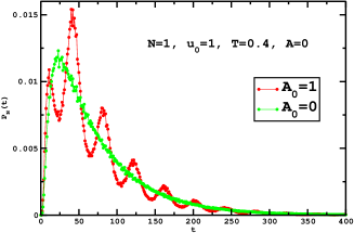
(a)

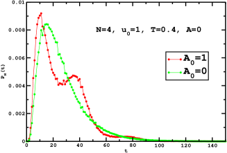
(b)

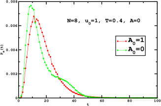
(c)

Figure 7: (Color online) The first passage time distribution $P_{N}(t)$ as a function of time for the parameter values of $U_{0}=1.0$, and $A=0$. The red and green lines are plotted when the external signal is turned on and off, respectively. In Figs. (a),(b) and (c), $N$ is fixed as $N=1$, $N=4$ and $N=8$, respectively.

The resonance profile can be observed better by looking at the relative ratios of the first passage time distribution functions with and without external periodic signal, i. e. taking the ratios of green and red lines in Fig. 8. It turned out that the ratio of the distribution is independent of the number of particles in the system as shown in Fig. 8a for single particle case and Fig. 8b for many particles case.

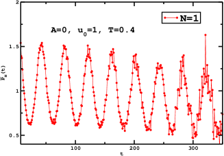
(a)

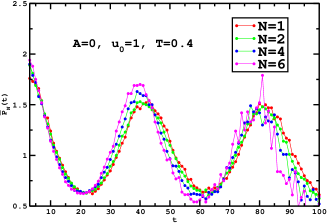
(b)

Figure 8: (Color online) The ratio of the first passage time distribution functions $\bar{P}_{N}(t)$. (a) The number of particle is fixed as $N=1$. (b) In the figure, $N$ is fixed as $N=1$, $N=2$, $N=4$ and $N=6$.

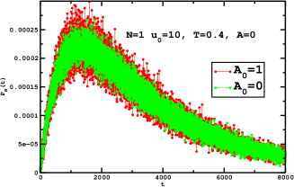
(a)

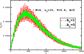
(b)

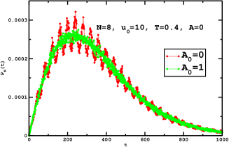
(c)

Figure 9: (Color online) The first passage time distribution $P_{N}(t)$ as a function of time in high barrier limit. In the figure, the parameters are fixed as $U_{0}=10.0$ and $A=0$. Figs. (a), (b) and (c) are plotted by considering one, four and eight particles, respectively.

In high barrier limit we see more peaks. In Figs. 9a, 9b and 9c, we plot the first passage time distribution time in high barrier limit. In the figures, the number of particles is fixed as $N=1$, $N=4$ and $N=8$, respectively. To compare with, we have plotted the distributions both in the presence of signal $A_{0}=1.0$ (red solid line) and in the absence of signal $A_{0}=0.0$ (green solid line). Only in the presence of signal that the the distributions shows the points of resonances.

To observe more the effect of the temperature dependence of $\gamma$ on the SR we have plotted the first passage time distribution functions in the presence of external force when $A=0$ and $A=1$ in the limit of small barrier height as shown in Fig. 10. In Figs. 10a, 10b and 10c, the number of particles is fixed as $N=1$, $N=4$ and $N=8$, respectively. The figures shows that the resonance is more pronounced when $\gamma$ is temperature dependent.

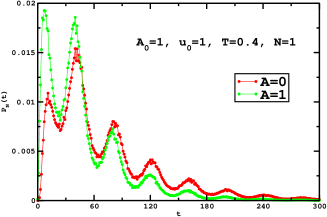
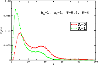
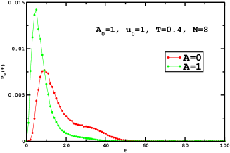
Figure 10: (Color online) The first passage time distribution $P_{i}(t)$ as a function of time in small barrier limit. In the figure, the parameters are fixed as $U_{0}=10.0$ and $A=0$. Figs. (a), (b) and (c) are plotted by considering one, four and eight particles, respectively.

IV.1 Signal to noise ratio

The signal to noise ratio can be studied via two state model. Employing two state model approach am14 , two discrete states $x(t)=\pm L_{0}$ are considered. Let us denote $n_{+}$ and $n_{-}$ to be the probability to find the particle in the right ($L_{0}$) and in the left ($−L_{0}$) sides of the potential wells, respectively. In the presence time varying signal, the master equation that governs the time evolution of $n_{\pm}$ is given by

$${\dot{n}}_{\pm}(t)=−W_{\pm}(t)n_{\pm}+W_{\mp}(t)n_{\mp}$$ (25)

where $W_{+}(t)$ and $W_{-}(t)$ corresponds to the time dependent transition probability towards the right ($L_{0}$) and the left (−$L_{0}$) sides of the potential wells. The time dependent rate am14 takes a simple form

$$W_{\pm}(t)=R\exp\left[\pm{L_{0}A_{0}\over U_{0}T}\cos(\Omega t)\right]$$ (26)

where $R$ is the Kramers rate for the particle in the absence of periodic force $A_{0}=0$. For sufficiently small amplitude, one finds the signal to noise ratio to be

$$SNR=N\pi R\left({L_{0}A_{0}e^{-T}\over U_{0}T}\right)^{2}$$ (27)

when $\gamma$ is temperature dependent and

$$SNR=N\pi R\left({L_{0}A_{0}\over U_{0}T}\right)^{2}$$ (28)

when $\gamma$ is constant. Here the rate can be found by substituting

$$R=N/T_{s}.$$ (29)

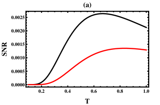
Figure 11: (Color online)(a) The $SNR$ as a function of $T$ for the parameter values of $A_{0}=0.1$, $U_{0}=2.5$, $U_{0}=2.0$ and $L_{0}=1.0$ from top to bottom, respectively for a variable gamma case. (b) The $SNR$ as a function of $T$ for the parameter values of $A_{0}=0.1$, $U_{0}=2.0$, $N=1.0$, $N=2$, $N=3.0$, $N=4$ and $L_{0}=1.0$ from top to bottom, respectively for a constant gamma case.

Before we explore how the SNR behaves as a function of $N$, we introduce additional dimensionless parameter: ${\bar{A}_{0}}=A_{0}L_{0}/U_{0}$, and for brevity we drop the bar hereafter. Fig. 11a depicts the plot for the SNR as a function of $T$ for the parameter values of $A_{0}=0.1$, $U_{0}=2.5$ and $U_{0}=2.0$ and $L_{0}=1.0$ from top to bottom, respectively for a variable gamma case. The SNR exhibits monotonous noise strength dependence revealing a peak at an optimal noise strength $T_{opt}$. $T_{opt}$ steps down as $A_{0}$ decreases. In Fig. 11b, the SNR as a function of $T$ is plotted for the parameter values of $U_{0}=2.0$, $N=1.0$, $N=2$, $N=3.0$, $N=4$ and $L_{0}=1.0$ from bottom to top, respectively for a constant gamma case and $A_{0}=0.1$. As shown in the figures the SNR increases with $N$.

IV.2 The power amplification factor

To gain more understanding of the SR of the Brownian particle, we consider the linear response of the particle to the small driving forces. Following the same approach as our previous work am24 , in the linear response regime, we find the power amplification power as

$$\eta=\left({\langle X^{2}\rangle}\over T\right)^{2}{{4R^{2}}\over{4R^{2}+\Omega^{2}}}$$ (30)

where $\left\langle X^{2}\right\rangle=\int X^{2}e^{{-U_{0}\over T}}dX/\int e^{{-U_{0}\over T}}dX$. In our case after some algebra we find

$$\left\langle X^{2}\right\rangle={L_{0}^{2}(-2T^{2}+e^{U_{0}/T}(2T^{2}-2TU_{0}+U_{0}^{2}))\over{U_{0}^{2}(-1+e^{U_{0}/T})}}$$ (31)

and as usual the rate $R=N/T_{s}$ where $T_{s}$ is given by Eq. (10) (variable $\gamma$) or Eq. (12) (constant $\gamma$).

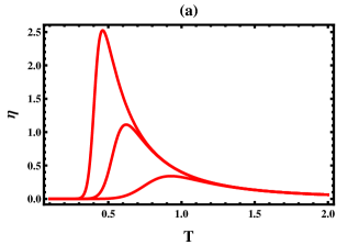
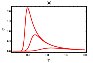
Figure 12: (Color online)(a) $\eta$ as a function of $T$ for the parameter values of $U_{0}=4$, $\Omega=0.004$, $\Omega=0.04$ and $\Omega=0.4$ from top to bottom, respectively for a variable $\gamma$ case. (b) $\eta$ as a function of $T$ for the parameter values of $U_{0}=4$, $\Omega=0.004$, $\Omega=0.04$ and $\Omega=0.4$ from top to bottom, respectively for a constant $\gamma$ case.

The spectral amplification $\eta$ as a function of $T$ is plotted in Fig. 12a for the parameter values of $U_{0}=4$, $\Omega=0.004$, $\Omega=0.04$ and $\Omega=0.4$ from top to bottom, respectively for a variable $\gamma$ case. The figure depicts that $\eta$ exhibits a pronounced peak at a particular $T_{opt}$. As $\Omega$ increases $\eta$ steps down and $T_{opt}$ shifts to the right. This is reasonable since resonance occurs when ${1\over T_{s}}=\pi\Omega$. As $\Omega$ steps up, $T_{s}$ should decreases in order to keep the resonance condition. However $T_{s}$ decreases only when $T$ increases. In Fig. 12b, we plot $\eta$ as a function of $T$ for the parameter values of $U_{0}=4$, $\Omega=0.004$, $\Omega=0.04$ and $\Omega=0.4$ from top to bottom, respectively for a constant $\gamma$ case. The same figures exhibits that the SNR is considerably lower for temperature dependent viscous friction case.

On the other hand for many particle cases $\eta$ as a function of $T$ is depicted in Fig. 13a for the parameter values of $U_{0}=4.0$, $\Omega=0.004$, $N=10$, $N=5$ and $N=1$ from top to bottom, respectively for a variable $\gamma$ case. The figure clearly exhibits that $\eta$ steps up as $N$ increases. The figure depicts that $\eta$ exhibits a pronounced peak at a particular $T_{opt}$. As $N$ increases $\eta$ steps up and $T_{opt}$ shifts to the left. This is plausible since resonance occurs when ${N\over T_{s}}=\pi\Omega$. Here since $\Omega$ is fixed, as $N$ increases, $T_{s}$ should increases to obey the resonance condition. However $T_{s}$ increases, only when $T$ decreases. In Fig 13b we plot $\eta$ as a function of $T$ for the parameter values of $U_{0}=4.0$, $\Omega=0.004$, $N=10$, $N=5$ and $N=1$ from top to bottom, respectively for a constant $\gamma$ case. The same figure exhibits that the peak of $\eta$ is smaller in comparison to that of variable $\gamma$ case.

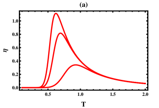
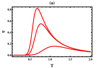
Figure 13: (Color online)(a) $\eta$ as a function of $T$ for the parameter values of $U_{0}=4.0$, $\Omega=0.004$, $N=10$, $N=5$ and $N=1$ from top to bottom, respectively for a variable $\gamma$ case. (b) $\eta$ as a function of $T$ for the parameter values of $U_{0}=4.0$, $\Omega=0.004$, $N=10$, $N=5$ and $N=1$ from top to bottom, respectively for a constant $\gamma$ case.

V Summary and conclusion

In the present work, a generic model system is presented which helps to understand the dynamics of excitable systems such neural and cardiovascular systems. The role of noise on the first passage time is investigated in detailed. Particularly, the role of temperature on the viscous friction as well as on the MFPT is explored by considering a viscous friction $\gamma$ that decreases exponentially when the temperature $T$ of the medium increases ($\gamma=Be^{-A}$) as proposed originally by Reynolds am10 . We show that the MFPT is smaller in magnitude when $\gamma$ is temperature dependent than temperature independent $\gamma$ case which is reasonable because the diffusion constant $D=T/\gamma=k_{B}Te^{T}$ is valid when viscous friction to be temperature dependent showing that the effect of temperature on the particle mobility is considerably high.

In this work first we study the MFPT of a single particle both for temperature dependent and independent viscous friction cases. The exact analytic result as well as the simulation results depict that the MFPT is considerably smaller when $\gamma$ is temperature dependent. In both cases the escape rate increases as the noise strength increases and decreases as the potential barrier increases. We then extend our study for $N$ particle systems. The first passage time $T_{N}$ for one particle out of $N$ particles to cross the potential barrier can be studied both analytically at least in the high barrier limit and via numerical simulation for any cases. It is found that $T_{N}$ is considerably smaller when the viscous friction is temperature dependent. For both cases, $T_{N}$ decreases as the noise strength increases and as the potential barrier steps down. In high barrier limit, $T_{N}=T_{s}/N$ where $T_{s}$ is the MFPT for a single particle. In general as the number of particles increases, $T_{N}$ decreases.

We then study our model system in the presence of time varying signal. In this case the interplay between noise and sinusoidal driving force in the bistable system may lead the system into stochastic resonance. Via numerical simulations and analytically, we study how the signal to noise ratio (SNR) and power amplification ($\eta$) behave as a function of the model parameters. $\eta$ as well as SNR depicts a pronounced peak at particular noise strength $T$. The magnitude of $\eta$ is higher for temperature dependent $\gamma$ case. In the presence of $N$ particle, $\eta$ is considerably amplified as $N$ steps up showing the the weak periodic signal plays a vital role in controlling the noise induced dynamics of excitable system

In conclusion, in this work, we explore the crossing rate and stochastic resonance of a single as well as many Brownian particles that move in a piecewise linear bistable potential by considering both temperature dependent and independent viscous friction cases. Although a generic model system is considered, the present study helps to understand the dynamics of excitable systems such neural and cardiovascular systems.

Acknowledgment.— We would like to thank Mulugeta Bekele for the interesting discussions we had. MA would like to thank Mulu Zebene for the constant encouragement.

References

- (1) H.A. Kramer. Physica 7, 284 (1940).
- (2) P. H¨anggi, P. Talkner and M. Borkovec, Rev. Mod. Phys. 62, 251 (1990).
- (3) P.J. Park and W. Sung, J. Chem. Phys. 111, 5259 (1999).
- (4) S. Lee and W. Sung, Phys. Rev. E 63, 021115 (2001).
- (5) P. H¨anggi, F. Marchesoni and P. Sodano, Phys. Rev. Lett. 60, 2563 (1988).
- (6) F. Marchesoni, C. Cattuto and G. Costantini, Phys. Rev. B, 57, 7930 (1998).
- (7) P. H¨anggi and F. Marchesoni, Rev. Mod. Phys. 81, 387 (2009).
- (8) K.L. Sebastian and Alok K.R. Paul, Phys. Rev. E 62, 927 (2000).
- (9) M. Bekele, G. Ananthakrishna, N. Kumar - Physica A 270, 149 (1999).
- (10) O. Reynolds, Phil Trans Royal Soc London 177, 157 (1886).
- (11) B. Lindnera, J. Garcia-Ojalvob, A. Neimand, L. Schimansky-Geier, Phys. Reports 392, 321 (2004).
- (12) W. Chen, M. Asfaw , Y. Shiferaw, Biophys J 102, 461 (2012).
- (13) M. Asfaw, E. A. Lacalle, Y. Shiferaw, Plos One, 8, e62967 (2013).
- (14) R. Benzi, G. Parisi, A. Sutera and A. Vulpiani, Tellus 34, 10 (1982).
- (15) L. Gammaitoni, P. H¨anggi, P. Jung and F. Marchesoni, Rev. Mod. Phys. 70, 223 (1998).
- (16) A. Neiman and W. Sung, Phys. Lett. A 223, 341 (1996).
- (17) P. Jung, U. Behn, E. Pantazelou, and F. Moss, Phys. Rev. A 46, R1709 (1992).
- (18) J. F. Lindner, B. K. Meadows, W. L. Ditto, M. E. Inchiosa, and A. R. Bulsara, Phys. Rev. Lett. 75, 3 (1995); Phys. Rev. E 53, 2081 (1996).
- (19) F. Marchesoni, L. Gammaitoni, and A. R. Bulsara, Phys. Rev. Lett. 76, 2609 (1996).
- (20) I. E. Dikshtein, D. V. Kuznetsov, and L. Schimansky-Geier, Phys. Rev. E. 65, 061101 (1996).
- (21) I. Goychuk and P. Hanggi, Phys. Rev. Lett. 91, 070601 (2003).
- (22) H. Yasuda et al., Phys. Rev. Lett. 100, 118103 (2008).
- (23) J. M. G. Vilar and J. M. Rubi, Phys. Rev. Lett. 78, 2886 (1997).
- (24) J. F. Lindner, M. Bennett, and K. Wiesenfeld, Phys. Rev. E 73, 031107
- (25) M. Asfaw and W. Sung, EPL 90, 3008 (2010).
- (26) M. Asfaw, Phys. Rev. E 82, 021111 (2010).
- (27) C. W. Gardiner. Handbook of Stochastic Methods for Physics, Chemistry and the Natural Sciences. Springer, Berlin, (1984).