Sooner than Expected: Hitting the Wall of Complexity in Evolution
Abstract
In evolutionary robotics an encoding of the control software, which maps sensor data (input) to motor control values (output), is shaped by stochastic optimization methods to complete a predefined task. This approach is assumed to be beneficial compared to standard methods of controller design in those cases where no a-priori model is available that could help to optimize performance. Also for robots that have to operate in unpredictable environments, an evolutionary robotics approach is favorable. We demonstrate here that such a model-free approach is not a free lunch, as already simple tasks can represent unsolvable barriers for fully open-ended uninformed evolutionary computation techniques. We propose here the “Wankelmut” task as an objective for an evolutionary approach that starts from scratch without pre-shaped controller software or any other informed approach that would force the behavior to be evolved in a desired way. Our focal claim is that “Wankelmut” represents the simplest set of problems that makes plain-vanilla evolutionary computation fail. We demonstrate this by a series of simple standard evolutionary approaches using different fitness functions and standard artificial neural networks as well as continuous-time recurrent neural networks. All our tested approaches failed. We claim that any other evolutionary approach will also fail that does per-se not favor or enforce modularity and does not freeze or protect already evolved functionalities. Thus we propose a hard-to-pass benchmark and make a strong statement for self-complexifying and generative approaches in evolutionary computation. We anticipate that defining such a “simplest task to fail” is a valuable benchmark for promoting future development in the field of artificial intelligence, evolutionary robotics and artificial life.
Keywords: Evolutionary Computation, Complexity, Artificial Neural Networks, CTRNN, Agent-Based Model, Stochastic Optimization
I Introduction
Robots are used more and more frequently in inherently unpredictable outdoor environments: Aerial search, rescue drones, deep-diving underwater AUVs and even extra-terrestrial explorative probes. It is impossible to program autonomous robots for those tasks in a way that one a-priori accommodates for all possible events that might occur during such missions. Thus, on-line and on-board learning, conducted for example by evolutionary computation and machine learning, becomes a significant aspect in those systems [1, 2, 3, 4]. Evolutionary Robotics has become a promising field of research to push forward the robustness, flexibility, and adaptivity of autonomous robots which combines the software technologies of machine learning, evolutionary computation, and sensorimotor control with the physical embodiment of the robot in its environment.
We claim here that evolutionary robotics operating without a-priori knowledge can fail easily because it suddenly hits an obscured “wall of complexity” with the current state of the art of unsupervised learning. While extremely simple (trivial) tasks evolve well with almost every approach that was tested in literature, already slightly more difficult tasks make all methods fail that are not a-priori tailored to the properties of the given task. As is well-known, there is no free lunch in optimization techniques [5]. The more specificly an optimizer is tailored to a specific problem, the more probable it is that it will fail for other types of problems. Thus, only open-ended, uninformed evolutionary computation will allow for generality in problem solving as required in long-term autonomous operations in unpredictable environments. For example, most studies in literature that have evolved complex tasks of cooperation and coordination in robots used pre-structured software controllers [6, 7] while most studies that have evolved robotic controllers in an uninformed open-ended way produced only simple behaviors, such as coupled oscillators that generate gaits in robots [8, 9, 10, 11] including simple reactive gaits [12], homing, collision avoidance, area coverage, collective pushing/pulling, and similar straight-forward tasks [13].
We hypothesize that one reason for the lack of success of evolving solutions for complex tasks, is the improbable emergence of internal modularity [14] in software controllers using open-ended evolution without explicitly enabling the evolution of modules. In an evolutionary approach it is possible to push towards modularity by pre-defining a certain topology of Artificial Neural Networks (ANNs) [15], by allowing to evolve a potentially unlimited number of modules within a pre-defined modular ANN structure [16, 17], or by switching between tasks on the time-scale of generations [18], which can then also be improved by imposing costs for links between neurons [19]. However, if modularity is not pre-defined and not explicitly encouraged by a designer, then a modular software controller will not emerge from scratch even if modularity is directly required by the task. While nature was capable of evolving highly layered, modularized and complex brain structures [20] by starting from scratch, evolutionary computation fails to achieve similar progress within reasonable time.
To support our claim we have searched for the most simple task that leads to failure of plain-vanilla uninformed unsupervised evolutionary computation starting from a 100% randomized control software without any interference (guidance) by a designer during evolution and without any a-priori mechanism or impetus to favor self-modularization. An easy way to define such a task is to construct it from two simple but conflicting tasks which are both easily evolvable in isolation for almost any evolutionary computation and machine learning approach of today. However, we require that the behavior that solves task 1 is the inverse of the behavior that solves task 2 (e.g., positive and negative phototaxis). Hence, once one behavior has been evolved the other behavior needs to be added together with an action selection mechanism. We have proposed a task that operates in one-dimensional space and as it is shown in the paper, it can be solved by a very simple pseudo-code and also by hand-coded ANNs. Compared to the classification scheme of [21] an agent, that solves the Wankelmut task, would be placed between vehicle #4 and vehicle #5 concerning the complexity of its behavior. Given that it operates in a one-dimensional space introduces a relation to vehicle #1. We anticipate that searching to define a “most simple task to fail” is a valuable effort for promoting future development in the fields of artificial intelligence, evolutionary robotics, and artificial life.
For simplicity we suggests simple plain-vanilla ANNs as an evolvable runtime control software in combination with genetic algorithms [22] or evolution strategies [23] as an unsupervised adaptation mechanism. For our benchmark defined here we accept either large fully connected and randomized ANNs as initialization as well as ANNs implementations that allow restructuring (adding and removing of nodes and connections) as a starting point. However, we consider all implementations that have special implementations to facilitate or favor modular networks as “inapplicable for our focal research question” because the main challenge in our benchmark task is to evolve modularization from scratch as an emergent solution to the task.
II Our Benchmark Task
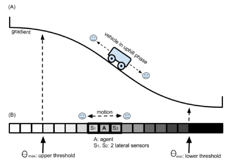
For the sake of simplicity we restrict ourselves to a very simple task that is hard to evolve in an open-ended, uninformed, and unguided way. As shown in Fig. 1, we assume an agent that moves in an environment expressing one single quality factor (e.g., height, water or air pressure, luminance, temperature) and which has to evolve a behavior that first makes the agent move uphill in this environmental gradient.
In the “uphill-walk” phase of the experiment the agent always should move in the direction of the sensor that reports the higher value of the focal quality factor. As soon as the agent reaches an area of sufficiently high quality (above a threshold ) the agent should switch its behavioral mode and start to seek areas of low environmental quality. In this “downhill-walk” phase the agent should always move towards the side where its sensor reports the lowest environmental quality value. After the agent has reached a sufficiently low quality area (below a threshold ) the agent should switch back to the “uphill-walk” behavior again.
We call the behavior that we aim to evolve “Wankelmut”, a term that expresses in German a character trait that always switches between two different goals as soon as one of the goals was reached. A "Wankelmut" agent is never satisfied and thus does not decide for one thing and does not stick with it. It is a variant of “the grass looks always greener on the other side”, a commonly found personality feature found in natural agents (from humans to animals) and, despite its negative perception in many cultural moral systems, has its benefits. It keeps the agent going, being explorative, curious and, never satisfied. That is exactly the desired behavior of an autonomous probe on a distant planet that needs to be explored.
In summary, the task is to follow an environmental gradient up and down in an alternating way, hence maximizing the coverage (monitoring, observation, patrolling) the areas between and . There are many examples that were evolved by natural selection [24]. In social insects (ants, termites, wasps, honeybees), foragers have first to go out of the nest and after they encountered food they switch their behavior and go back to the nest. After they have unloaded the food to other nest workers they go outwards to forage again [25]. Often environmental cues and gradients are involved in the homing and in the foraging behaviors (sun compass, nest scent, pheromone marks) and are exploited differently by the workers in the outbound behavioral state compared to the inbound behavioral state [26]. Other biological sources of inspiration are animals following a diurnal rhythm (day-walkers and night-walkers). In an engineering context the rhythm might be imposed by energy recharging cycles, water depths, or aerial heights in transportation tasks by underwater vehicles or aerial drones.
Figure 1B shows that we de-complexified the benchmark task to a one-dimensional cellular space of cells in which always one cell of index is occupied by the agent which has state . The environmental gradient is produced by the Gauss error function
| (1) |
whereby the quality of every cell is modeled as
| (2) |
In every time step , the agent has access to two lateral sensor readings which are modeled as
| (3) |
and
| (4) |
The agent changes its position based on these sensor readings:
| (5) |
whereby the agent’s position is restricted by the boundaries of the simulated world. Its motion () is restricted to a maximum of 1 step to the left or to the right of the agent’s current position.
Initially the agent is in uphill state which means it should move uphill. If the agent’s local then the state is changed to downhill and if the agent’s local then the agent’s state is changed back to uphill.
III Known solutions
The Wankelmut task is actually very simple to solve, as it is just a greedy uphill walk in combination with a greedy downhill walk complemented by a threshold-dependent switch.
A simple algorithm, such as the python-like pseudo code in Fig. 2 solves the task with a few lines of code in the desired reactive and optimal way. We used this code to calculate the “maximum reachable fitness” in our quantitative analysis section. The variable state and the constant theta define the agent’s own state and the thresholds at which it should switch from one behavior to the other and vice versa. The two variables S_l and S_r hold the current sensor values at the left and at the right side of the agent and report values between and . The function set-actuators() drives the robot to the left with positive numbers and to the right with negative numbers used as the only argument. In our study we use this simple hand-coded solution as a reference and investigate how close the evolved control software gets to the fitness values achieved by this simple but optimal solution.
# the agent’s initialization is executed at the beginning

def agent_init():
  state=1     # state: +1 is uphill, -1 is downhill state
  theta=0.95  # thresholds are at .05 and .95 (symmetrical setting)

# the agent’s action procedure is executed every time step

def agent_act():
  if (S_l*state)>(S_r*state):
    set-actuators(state)
  else:
    set-actuators(state*-1)
  if (mean(S_l,S_r)*state)>theta:
    state=state*-1
It is noteworthy that this reactive solution of the Wankelmut task would operate in gradients of any shape and size in an optimal way as long as gradients are strictly monotone between the two points and . While we used a sigmoid-type non-linear gradient by using the Gauss error function, our hand-coded solution, presented as pseudo-code in Fig. 2, works optimally also in linear gradients of any size and steepness.
IV Evolvable Agent Controllers
Hand-Coded Artificial Neural Network
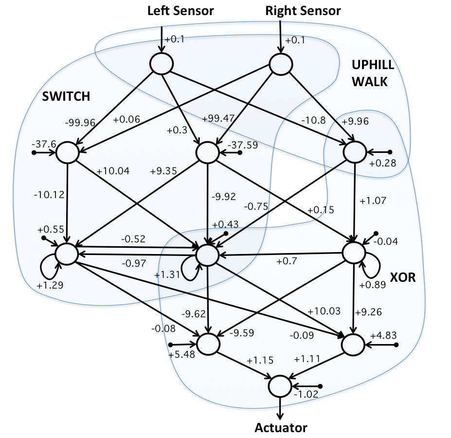
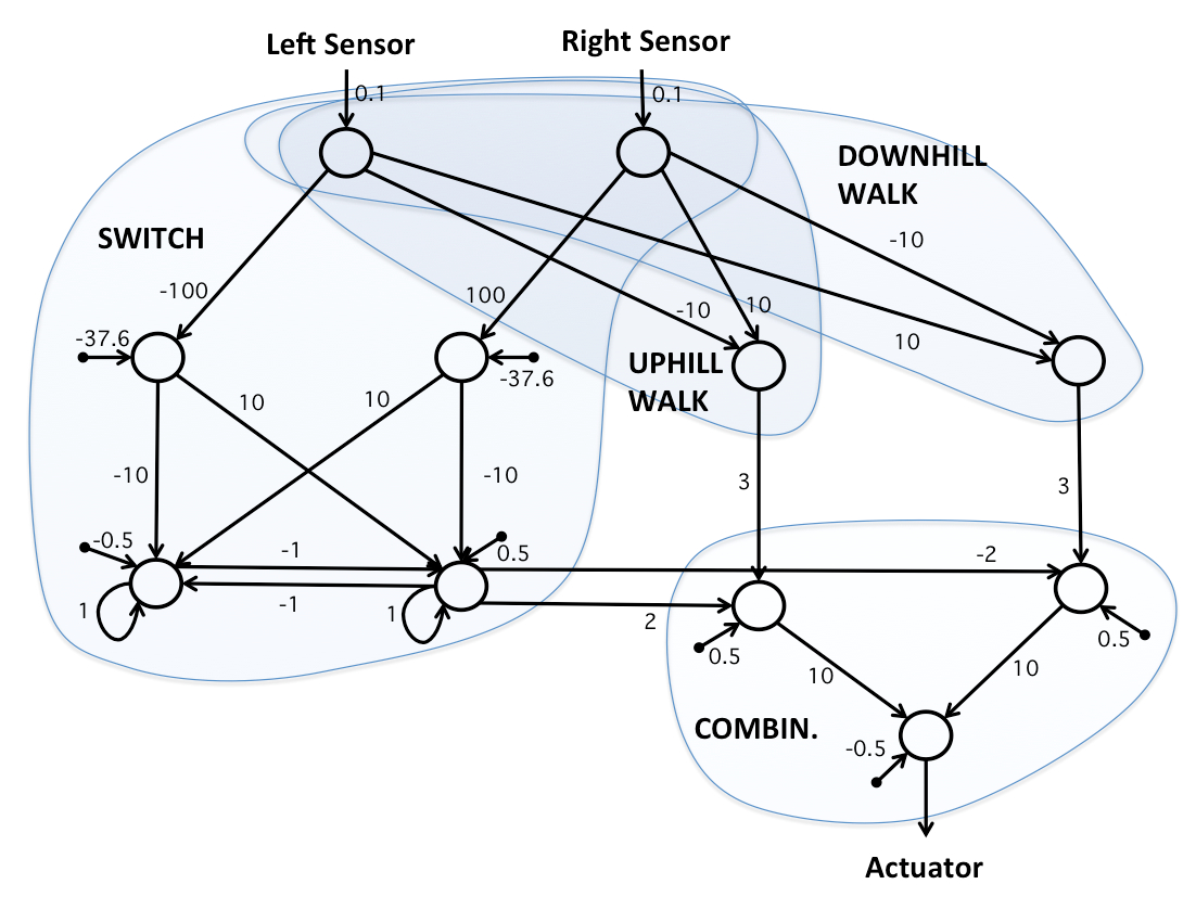
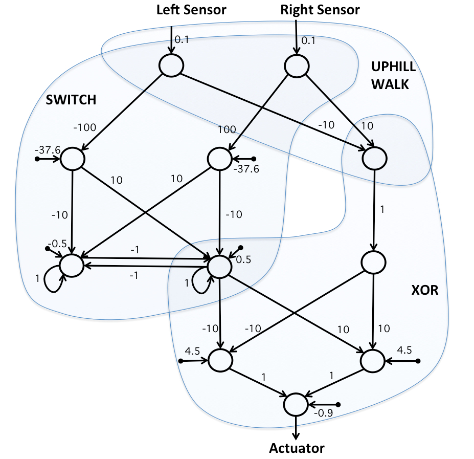
In order to make sure that the topology of our neural networks that are evolved is sufficient for solving the problem, we designed hand-coded neural networks. For the activation function, we used a sigmoid function: . Fig. 3 shows two example hand-coded neural networks. In Fig. 3, an uphill and a downhill walk subnetworks and a switch subnetwork are designed. The switch keeps the current state of the controller and when the inputs pass the thresholds, it switches to the other state. Finally in the last subnetwork, the information from the switch is used to choose between uphill and downhill walk. Fig. 3, has a slightly different design where the output of the switch and an uphill walk subnetworks are combined by using a logical xor subnetwork. The number of the nodes in both networks are the same, however, the number of weights used in the second example is lower. The topology of the neural network to be evolved is chosen in a way that it covers the second hand-coded network. The number of the nodes chosen for the CTRNN network to be evolved is chosen so that it covers both networks.
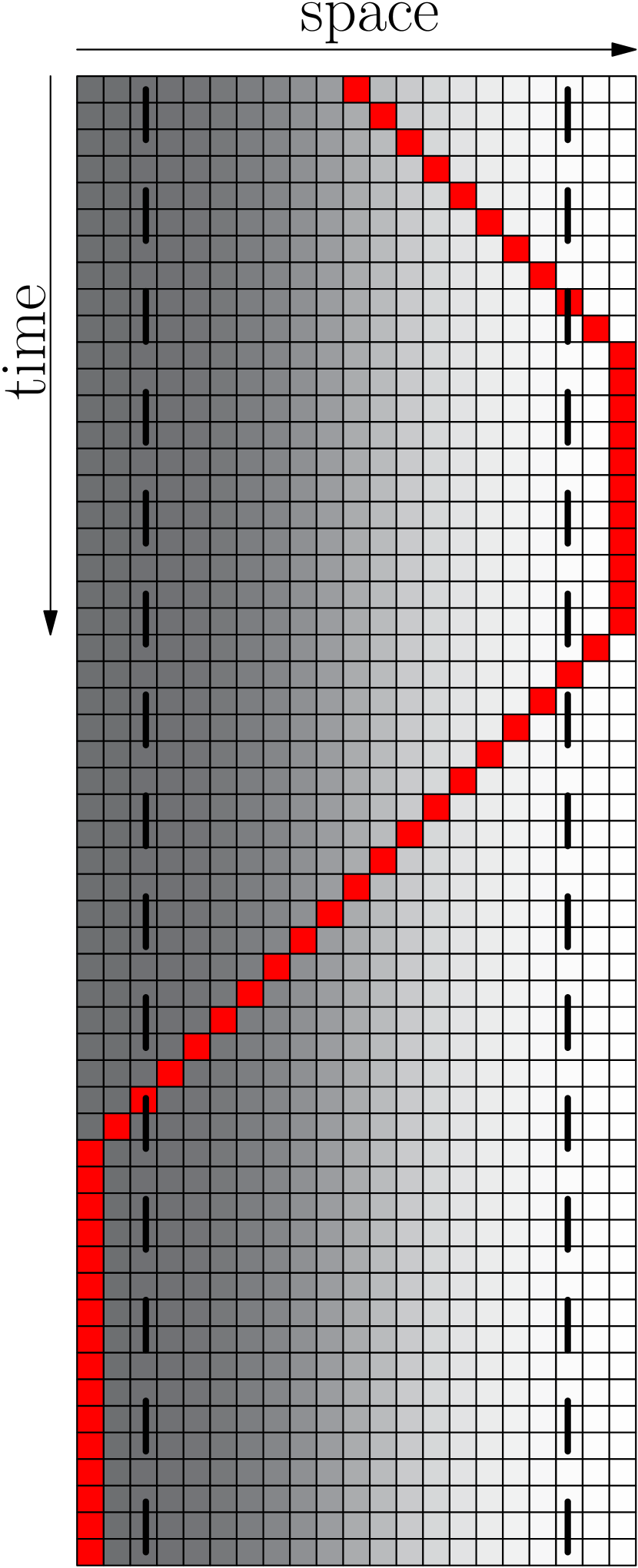
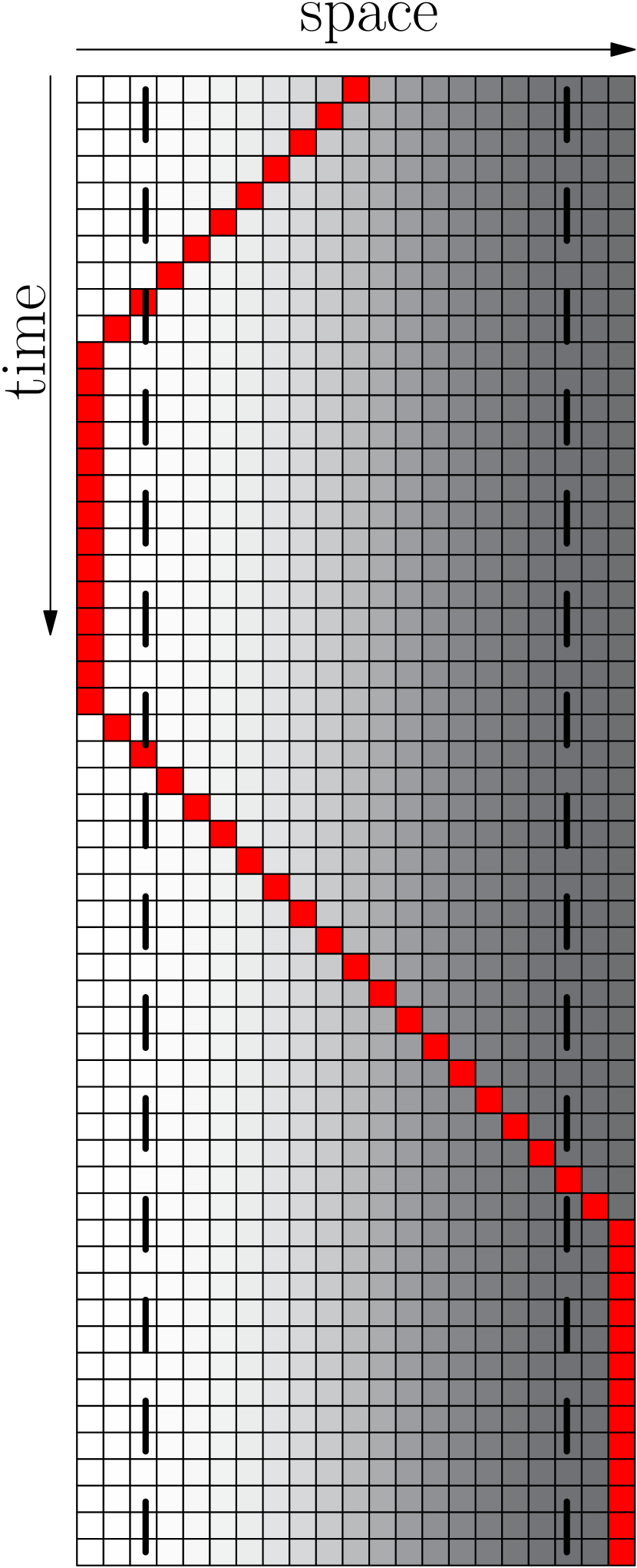
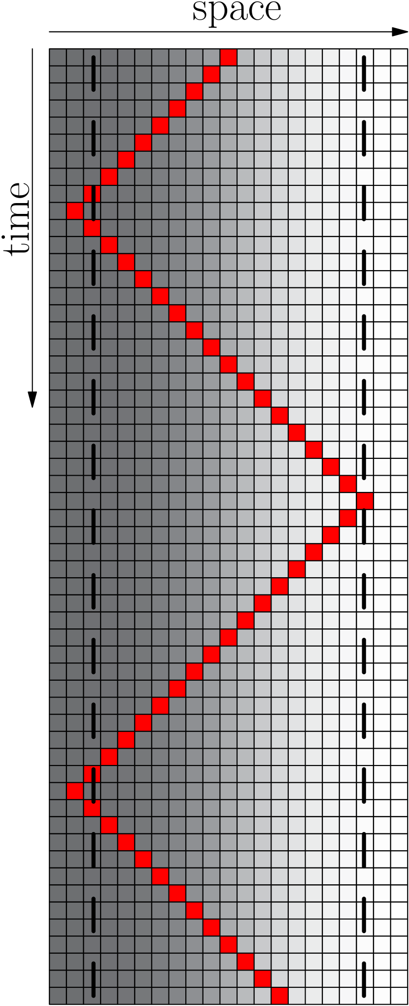
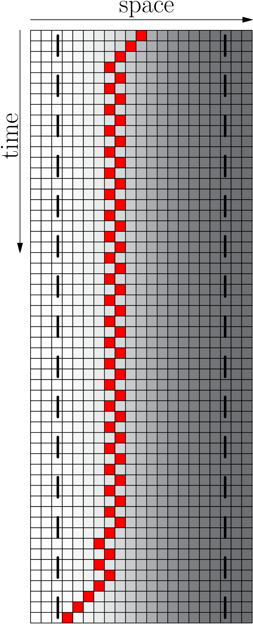
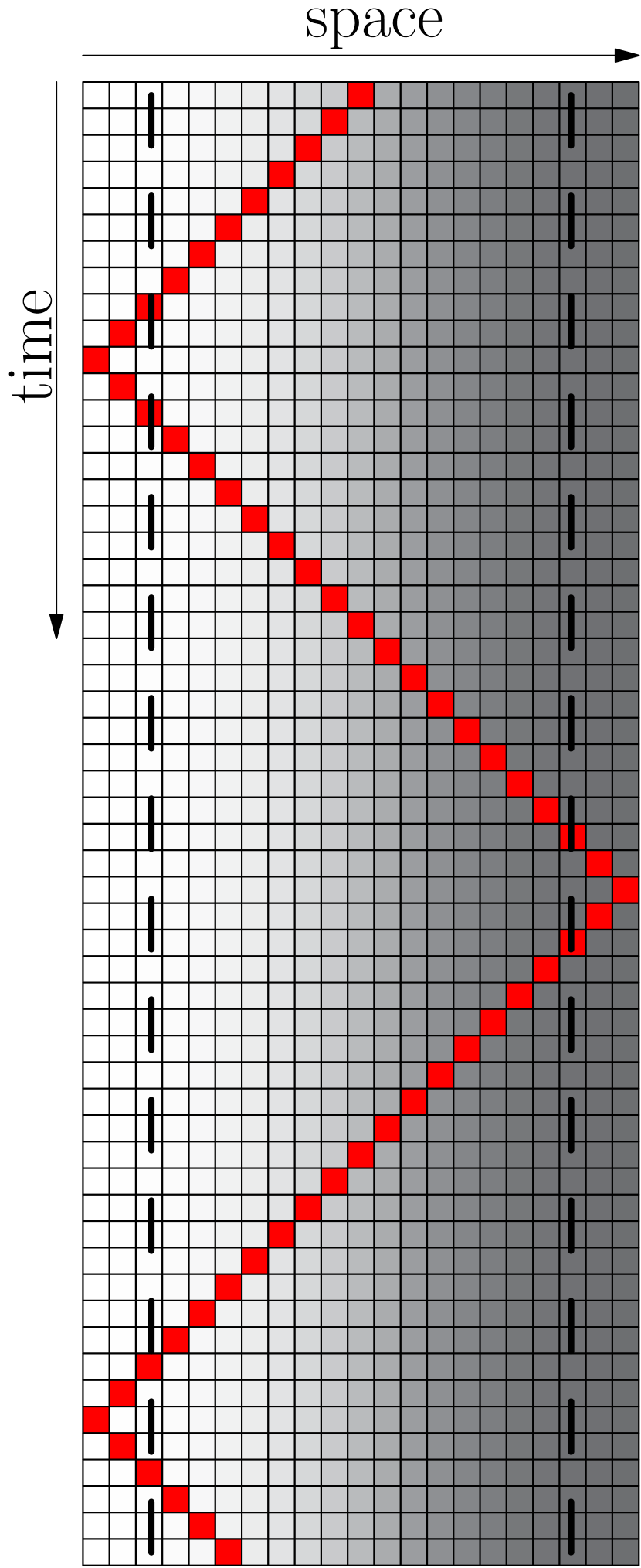
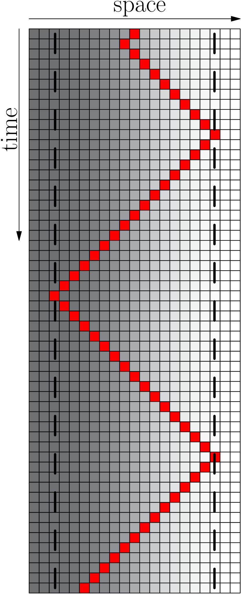
The behaviors of an agent controlled by both networks are the same. The behaviors in two different environments are demonstrated in Fig. 11 , 11. Fig. 11, shows the behavior when the quality of the environment is increasing from left to right. Fig. 11, shows the behavior when the quality of the environment is decreasing (The quality of the environments are represented in gray-scales).
I Simple Artificial Neural Network
Our simple approach made use of recurrent artificial neural networks. The used activation function is a sigmoid function: . We had 11 neurons with two in the input layer, three in a first hidden layer, another three in a second hidden layer, two in the third hidden layer, and one in the output layer. Each neuron in the second hidden layer had a link to itself (loop) and an input link from each of the neighboring nodes in addition to the links from the nodes in the previous layer. Weights were randomly initialized with random uniform distribution from the interval .
II Continuous-Time Recurrent Neural Networks
In a second approach we used Continuous-Time Recurrent Neural Networks (CTRNNs) which are Hopfield continuous networks with unrestricted weights matrix inspired by biological neurons [27]. A neuron in the network was of the following general form:
| (6) |
where was the state of the th neuron, was the neuron’s time constant, was the weight of the connection from the th to th neuron, was a bias term, was a gain term, was an external input, and was the standard logistic output function.
The weights were randomly initialized. By considering the study of the parameter space structure of CTRNN by [28], the values of the s were set based on the weights in a way that the richest possible dynamics were achieved. We used 11 nodes where two nodes received the sensor inputs and one node was used as the output node determining the direction of the movement (right/left).
III How we expect that evolution to solve the Wankelmut task
Although the task might seem to be solved in a straight forward way, a number of different strategies can be taken by an optimal controller. Also notice that we tested our agents in two types of environments in the following: One environment with the maximum at the left hand side and another environment with the maximum at the right hand side.
An intuitive solution is a controller that can go uphill or downhill along the gradient with a 1-bit internal memory for determining the current required movement strategy (uphill or downhill). The internal memory switches its state when the sensor values reach the extremes (defined thresholds). The initial state of the memory should indicate the uphill movement. Hence, a controller requires only this 1-bit internal memory. The comparison between the instant values of the sensors then determines the actual direction of the movement in each step. We would consider such a solution as a “correct” solution, as it basically resembles the pseudo-code given in Fig. 2. We assume that our chosen topology of the ANNs allow in principle to evolve the required behavior based on one internal binary state variable. Our simple ANN was a recurrent network and had two hidden layers with three nodes each. These two hidden layers should have provided enough options to evolve an independent (modular) uphill and downhill controller in combination with a 1-bit memory and an action selection mechanism. Similarly, for the CTRNN approach we have used nine neurons and any topology between them is allowed.
Another solution to solve the task can be done in the following way: The controller starts by deciding about the initial direction of the agent’s movement to the right or left depending on the initial sensor value. In the following it continues a blind movement (i.e., not considering the directional information of the sensor inputs) until extreme sensor values are perceived and then switches the direction of the agent. Also here an internal 1-bit state variable is required to keep the direction of the agent’s movement.
There is even another solution possible. As our environment does not change in size, the controller does not even need to consider the sensor values at any time except the first time step: In this strategy, the robot has to initially classify the environment and then the remaining task can be completed correctly by choosing one of two “pre-programmed” trajectories. In this solution, the sensor information is only used at the first time step but instead, a more complicated memory (more than 1-bit) is needed to maintain the oscillatory movement between the two extremes. This is not a maximally reactive solution meaning that it partially replaces reactivity to sensor inputs with other mechanisms; i.e., using extra memory and pre-programmed behaviors. Such a solution would not work in the way we expect it to work in other environments (e.g., changed size of the gradient). Such a controller might achieve the optimal fitness in our evolutionary runs, but a post-hoc test in a slightly different environment would identify that it generates sub-optimal behavior. Thus, it does not represent a valid solution for the Wankelmut task. A post-hoc test that detects such a solution could be done by changing the size or the steepness of the environmental gradient or by using a Gaussian function (bell curve) instead of the Gauss error function (erf) with randomized starting positions: In this case the agent should oscillate only in the left or in the right half of the environment, depending on its starting position, to implement a true reactive solution to the Wankelmut task.
Other solution strategies can also concern the switching condition, for example the switching may occur based on the extreme values of the sensors (defined thresholds), the difference between the two sensor values, or the fact that at the boundaries of the arena, the sensor values may not change even if the agent attempts to keep moving in the same direction, as we do not allow the agent to leave the arena.
Here, we are interested in controllers which are maximally reactive, meaning that they base their behaviors on the reacting to sensor values instead of scheduling pre-programmed trajectories. The usage of memory in such controllers is minimized since memory is replaced by reactivity to sensors wherever it is possible. In our case, a valid controller is expected to need a sort of 1-bit memory (that is not replaceable by reactivity to sensors) to keep track of the direction of its movement. Solutions that use extra memory for scheduling their pre-programmed trajectories are considered invalid.
We are aware that the “creativity” of evolutionary computation cuts both ways. It can surprise by “cheap tricks” that maximize fitness without producing the desired agent behavior. Post-hoc, such a result is usually considered to be an attribute of bad fitness function design [29]. Therefore, we define several fitness functions and have tested two software control techniques (ANN and CTRNN) using each fitness function in 30 evolutionary runs per setting as it is described in the following quantitative analysis section.
V Quantitative analysis
I Fitness Evaluation
In the experiments reported here, we have used different fitness regimes based on the number of the correct switches and the positioning of the agents. In order to define the different fitness regimes, three types of rewards are considered:
-
•
Rewarding for switch: rewarding point for every correct switch: , where is the number of correct switches over the whole period of the experiment.
-
•
Cumulative rewarding for positions: rewarding based on the state and the environmental quality of the positions of the agent accumulated over the whole period of the experiment:
. That means that an agent in uphill mode () is rewarded the current environmental quality of its position and an agent in downhill mode () is rewarded the current quality multiplied by -1. In consequence, agents in uphill mode are rewarded positively for locating themselves in high-quality regions and agents in downhill model for locating themselves in low-quality regions. -
•
Instant rewarding for final position: rewarding based on the state and the environmental quality of the final position of the agent: , where is the period of experiment. In this case, the reward is given for the final position of the agent. The exact value of the reward depends on the final state of the agent, but in any case a higher reward is given if the agent is closer to the next correct switch. That means, if the agent is in the uphill mode, a higher reward is given if it is higher up the hill and if it is in the downhill mode, a higher reward is given if it is more down the hill.
By giving different weights to the three types of the rewards, the fitness function is defined as follows:
| (7) |
where , , and are parameters of the fitness function representing the weights for every type of the rewards.
In this study, the following fitness regimes are investigated:
-
1.
Switch: , rewarding only for correct switches.
-
2.
Cumulative , only cumulative rewarding for positions.
-
3.
Instant+Switch: , rewarding for correct switches as well as instant rewarding for final position.
-
4.
Cumulative+Switch: , rewarding for correct switches as well as cumulative rewarding for positions over the whole period.
II Evolving Solutions in Various Scenarios
In the following, we were using a number of evolutionary setups (scenarios) and investigated the resulted controllers achieved by evolution in each setup. Two different controller types, ANN and CTRNN were used. In all the scenarios, every controller ran for 250 time-steps unless otherwise stated. Results were pooled from 30 independent runs for each scenario.
We used a simple genetic algorithm [22] with proportionate selection based on fitness and elitism of one. The population size was set to 150 and we ran for 300 generations. A genome for the ANN consisted of 41 genes each encoding a connection weight between the nodes. The weights are randomly initialized between . A genome in the CTRNN consisted of 121 genes for the weights of the connections, 11 genes for the values of and 11 genes for the values of every node. The weights and values are randomly initialized in the range of and respectively. The values of s are set based on the weights such that the richest possible dynamics is achieved, as described in [28]. We did not use a recombination operator. In ANN, the weights are mutated with a rate of where a random value in is added to the weight. In CTRNN the mutation rate if for weights and a random and are mutated at a time. The values are changed in the range of for weights and , and in the range of for . Table 1 summarizes the evolutionary parameters.
| parameter | ANN | parameter | CTRNN |
|---|---|---|---|
| population size | 150 | population size | 150 |
| number of genes | 41 | number of genes (weights) | 121 |
| number of genes () | 11 | ||
| number of genes () | 11 | ||
| init. range (weight) | init. range (weight) | ||
| init. range () | |||
| init. range () | as in [28] | ||
| mutation rate | 0.3 | mutation rate (weights) | 0.1 |
| mutation rate (, ) | a random one at a time |
II.1 Single Environment vs. Double Environment, Mean fitness versus Minimum Fitness
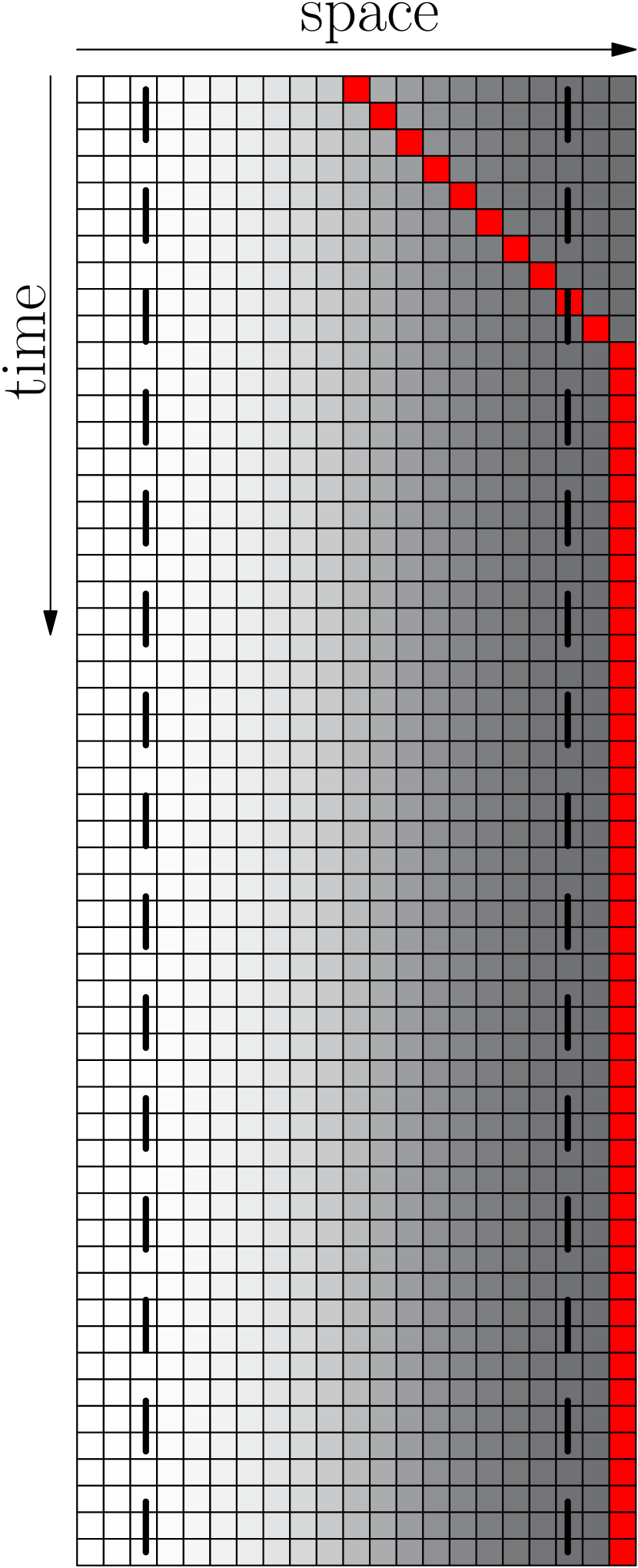
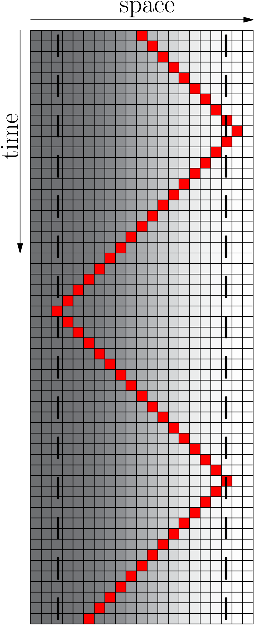
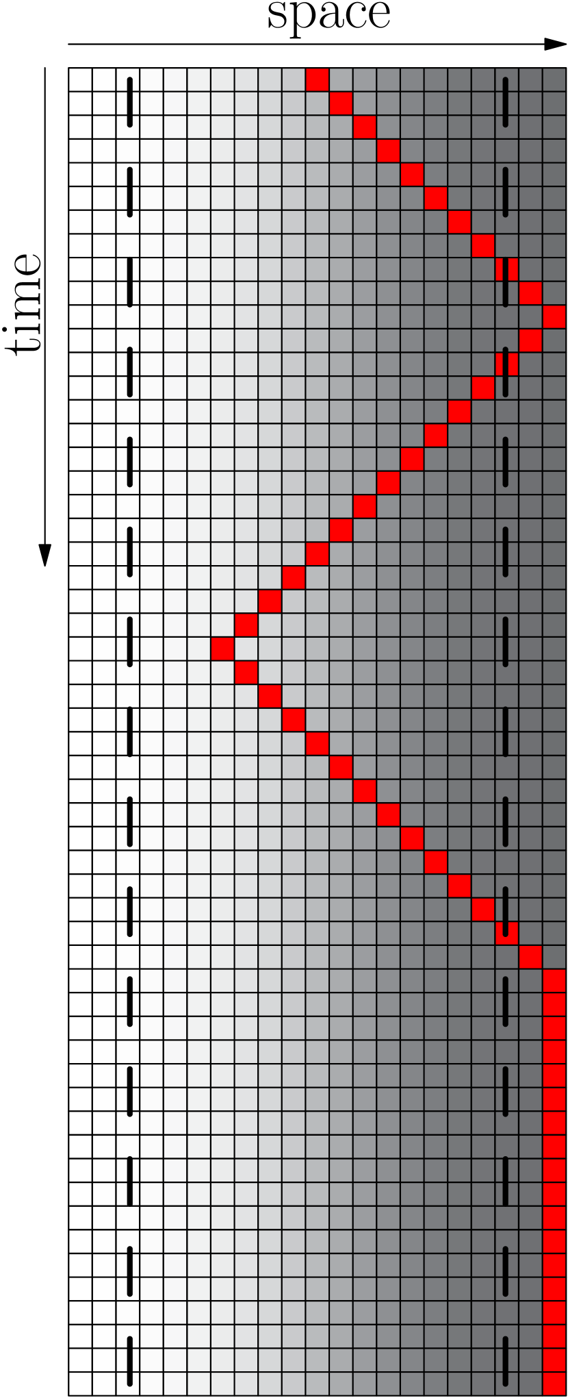
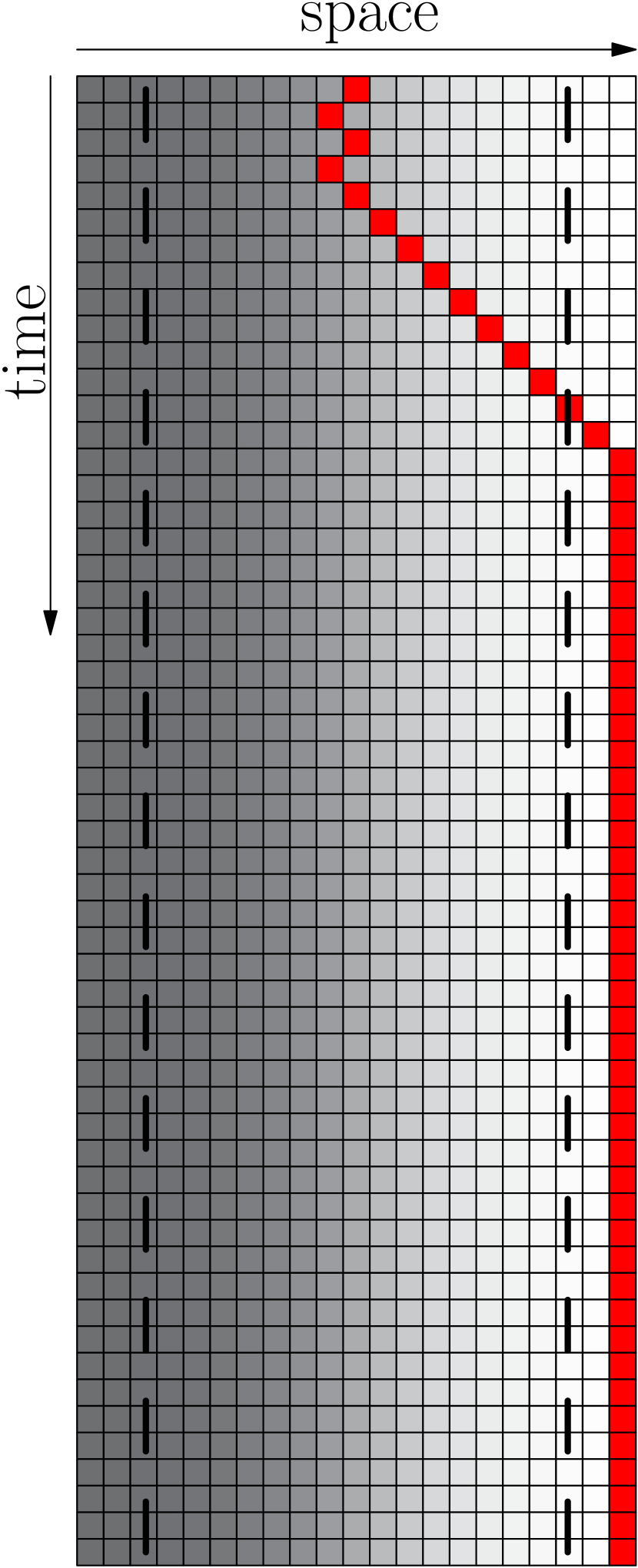
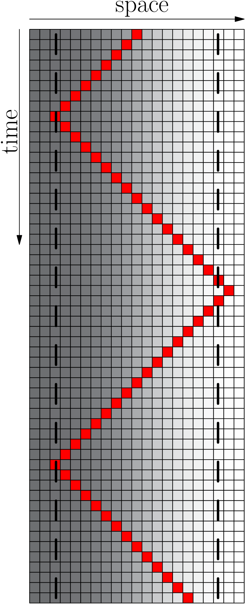
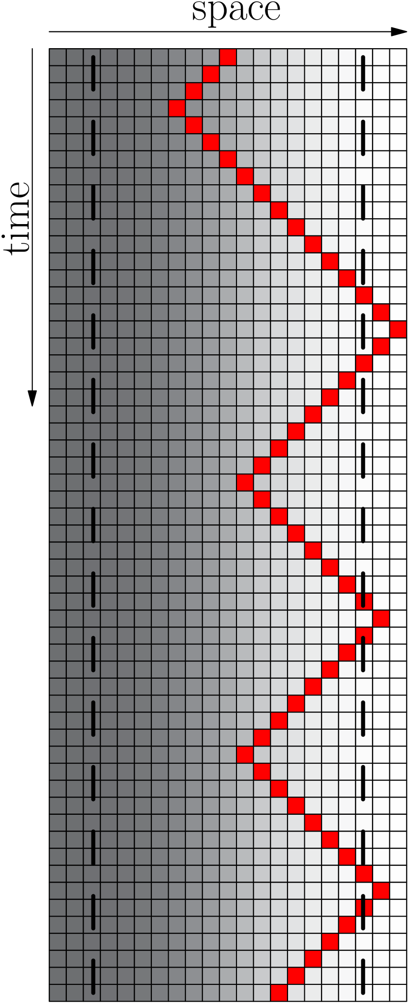
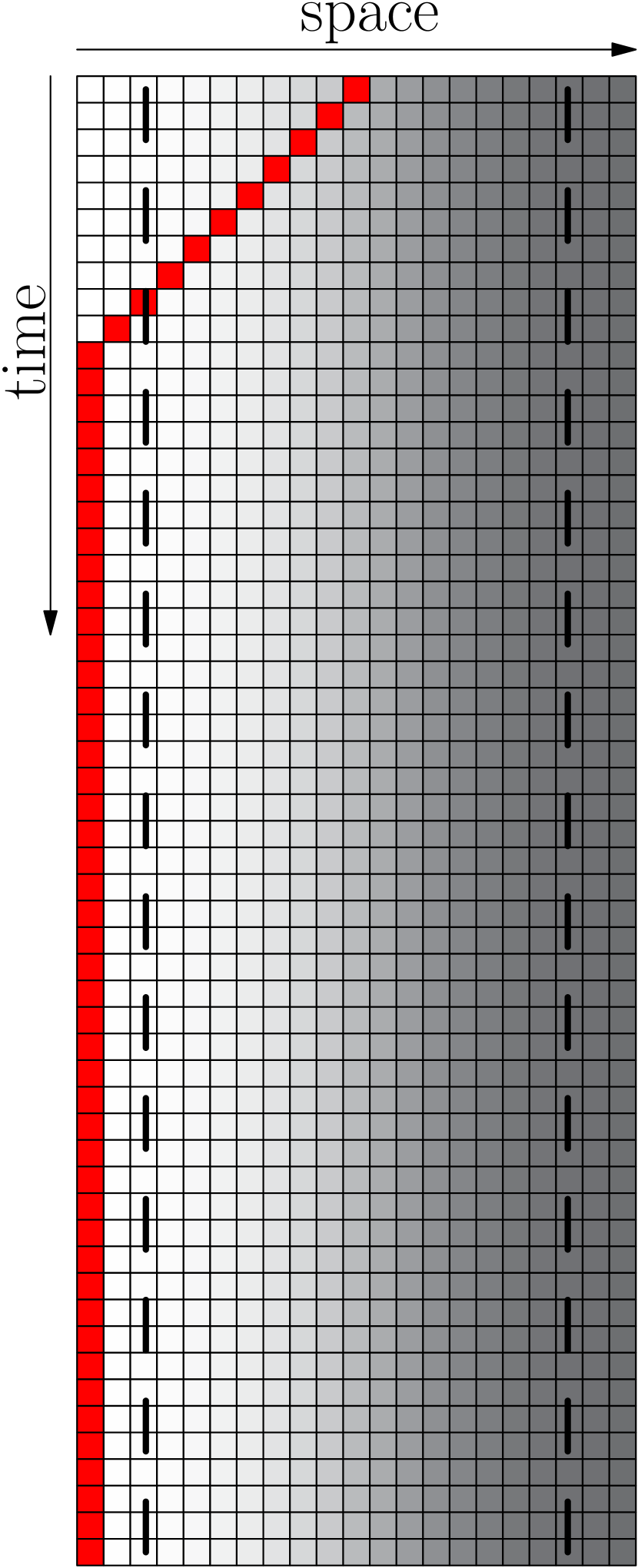
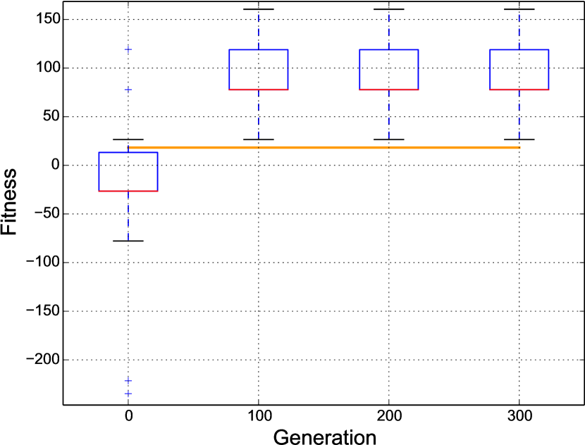
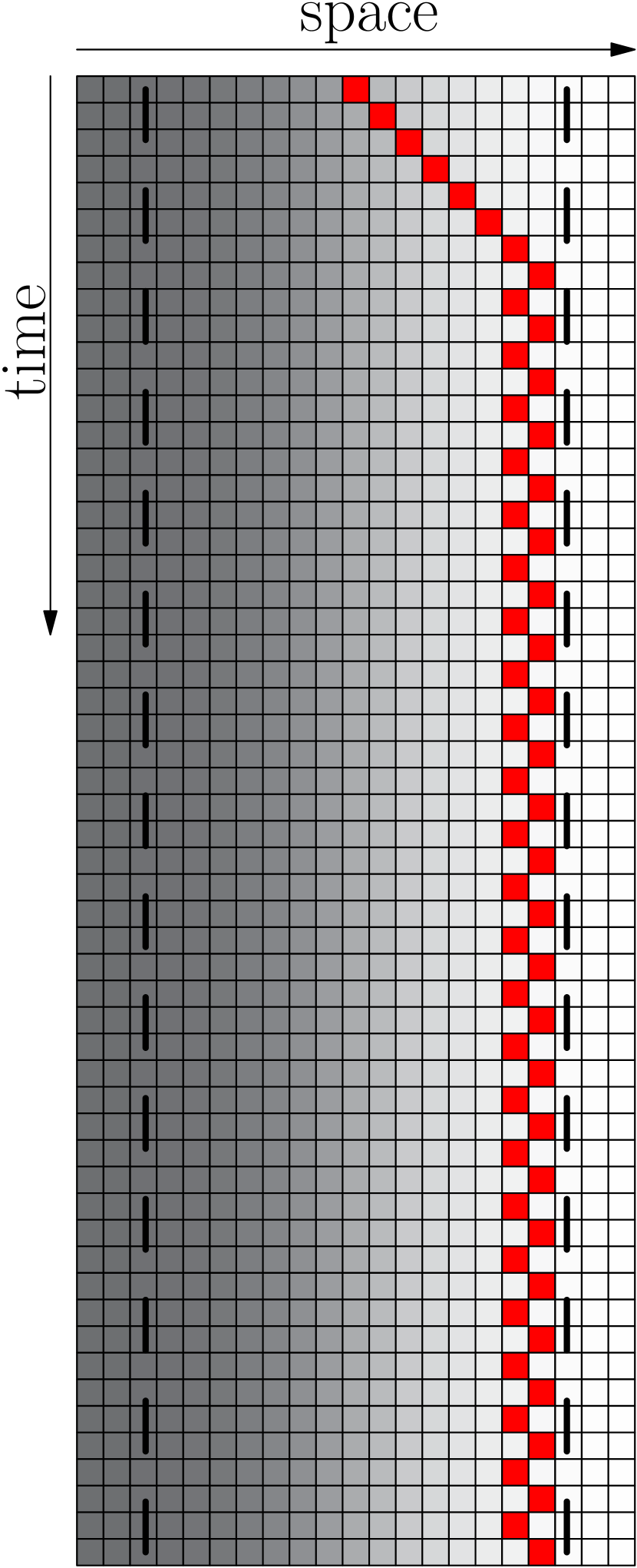
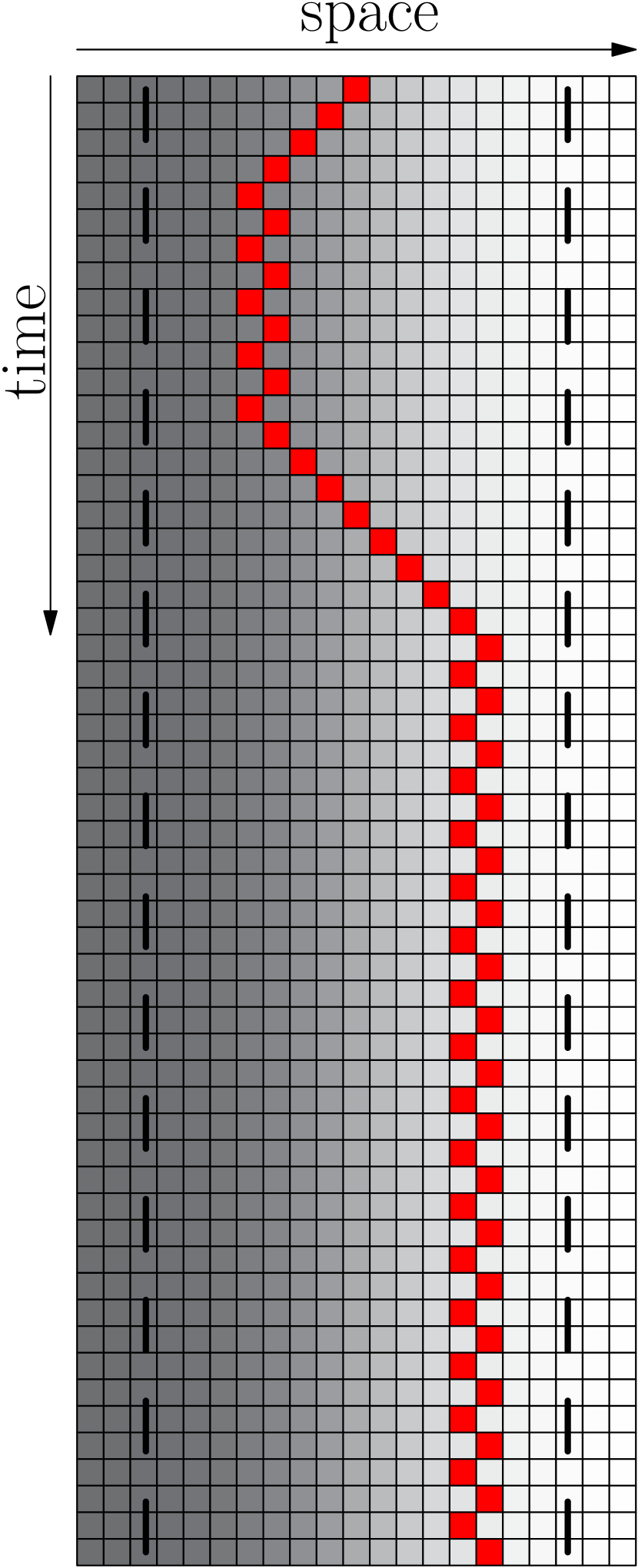
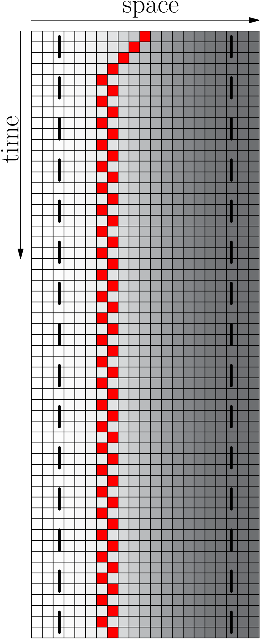
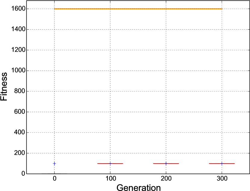
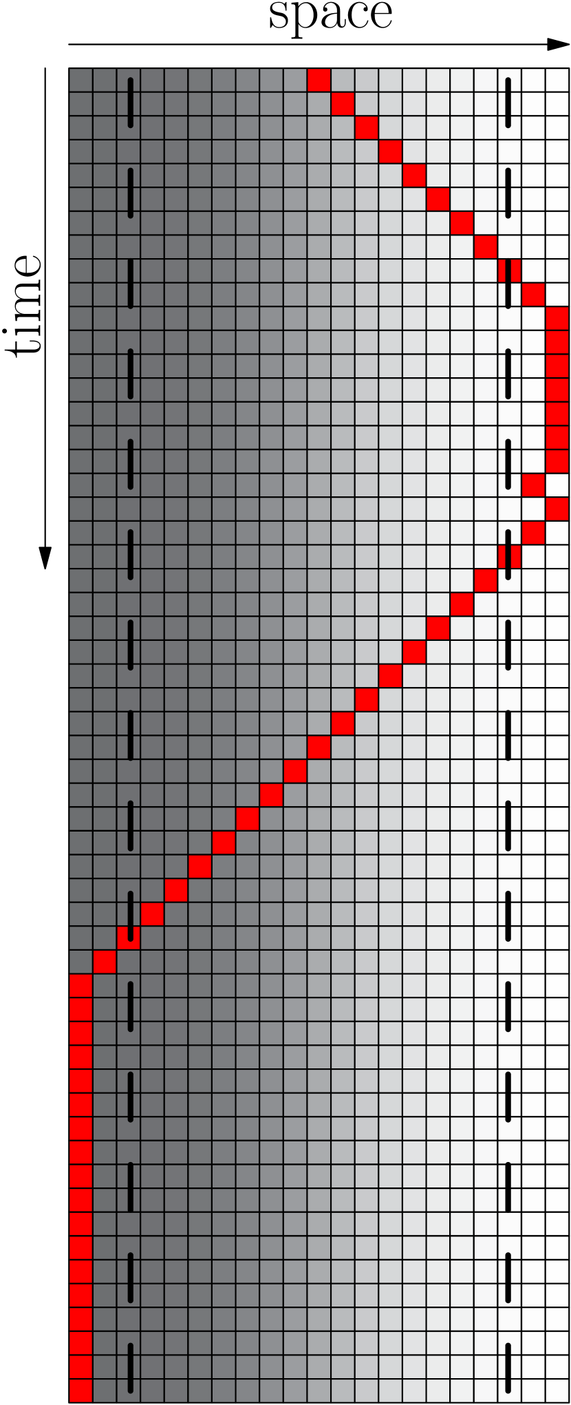
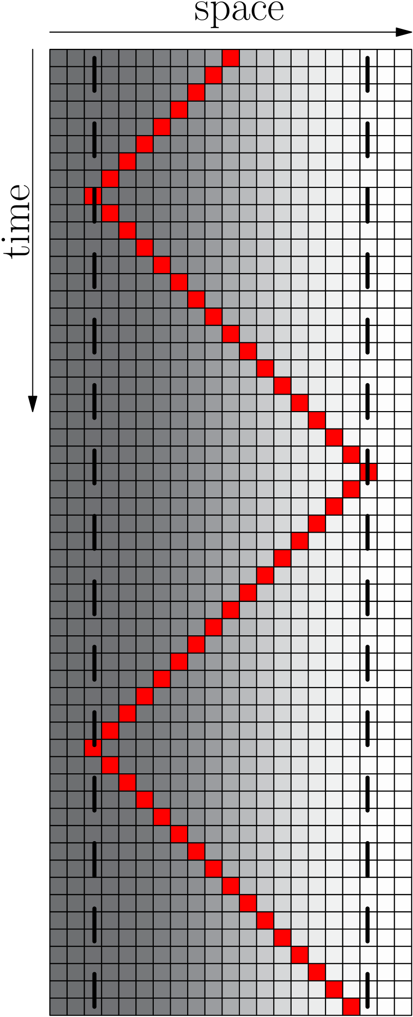
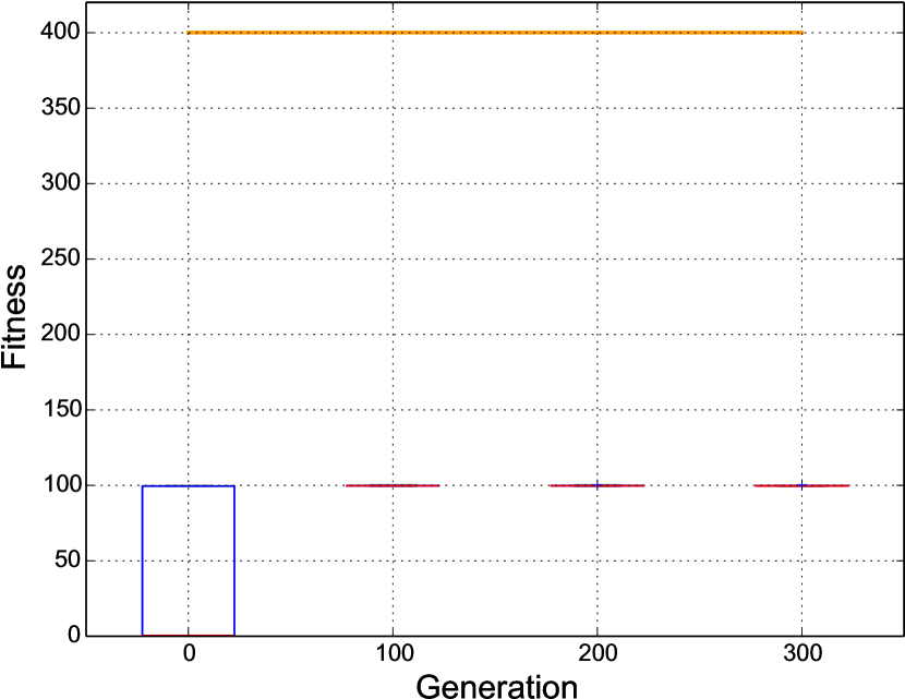
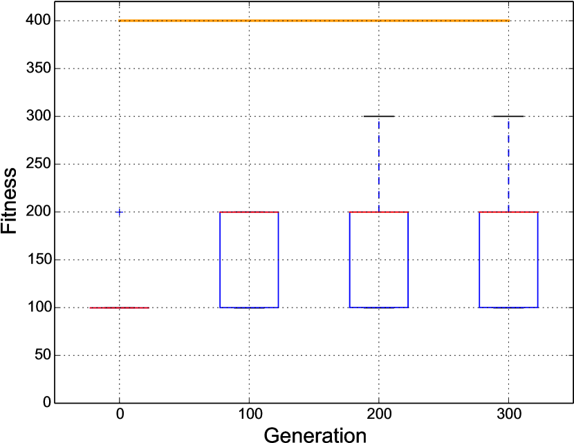
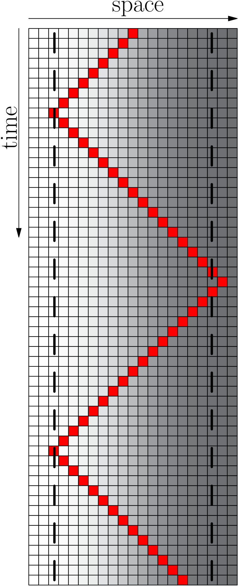
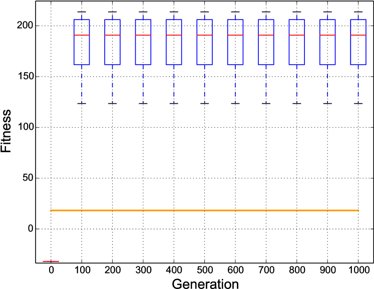
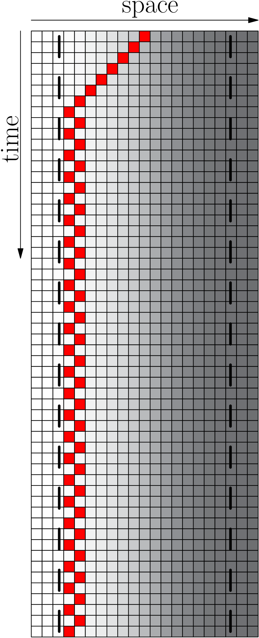
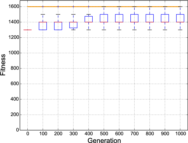
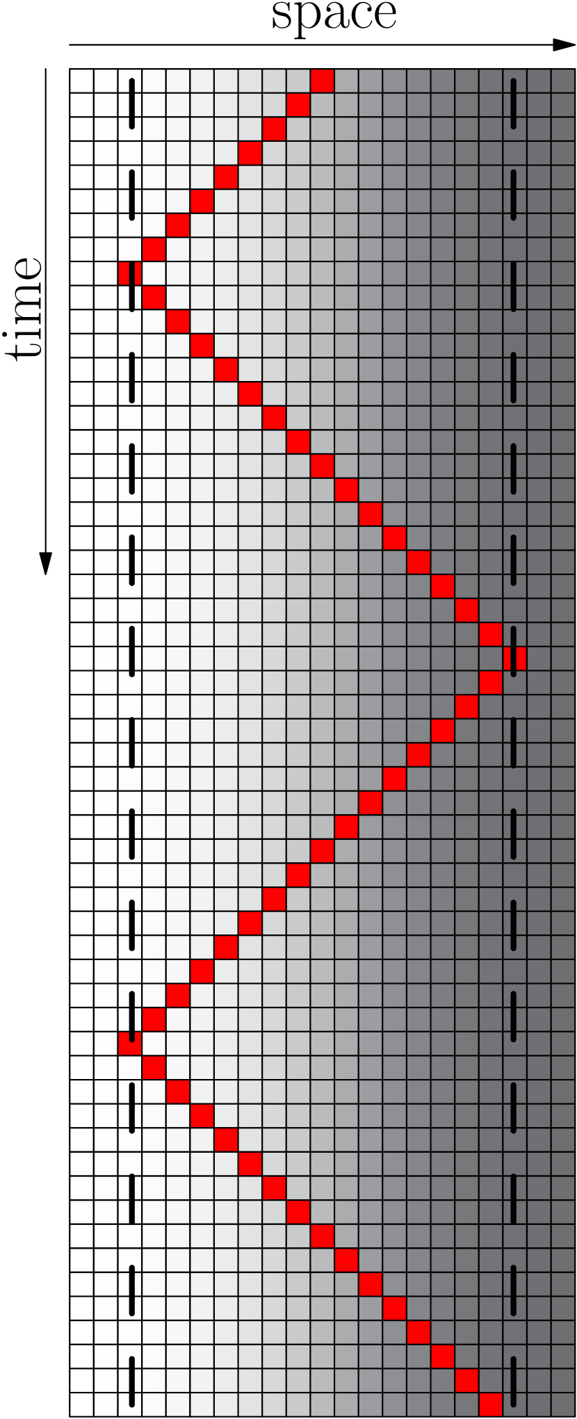
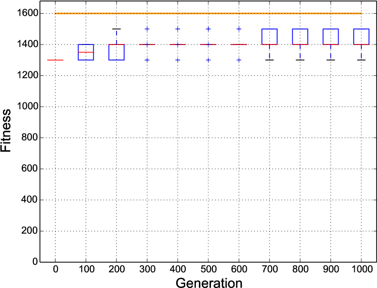
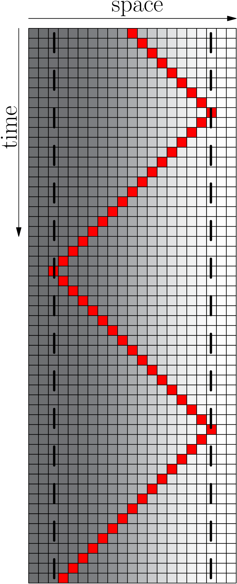
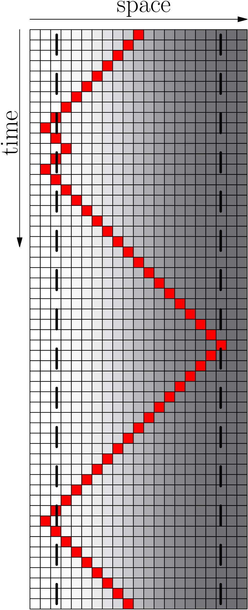
At first we evaluated the performance of evolution in a fixed environment, like it is depicted in Fig. 1. We found that evolution could quickly converge to a sort of pre-programmed trajectory (see Fig. 4 and Fig. 4) that achieved very high fitness (see Fig. 4 and Fig. 4) but was non-reactive as it was not considering sensor inputs in the wanted way: A post-hoc test of the best evolved genomes in a flipped environment, where the gradient pointed to the other side, was failed by both evolved controller types, clearly indicating that no reactive Wankelmut behavior has evolved (see Fig. 4 and Fig. 4). The trajectories in both post-hoc runs show some difference to the runs in the environment that was used in evolution, this indicates that some sensor-input was affecting the behavior but not in the desired way: The agents still started off in the wrong direction and also the oscillations ceased after some time.
As this approach was not yielding the wanted reactive Wankelmut behavior, we decided to evaluate each individual genome twice: One time the gradient pointed uphill to the left and one time it pointed uphill to the right side. The fitness function in all the three scenarios used the Switch fitness regime which is described as .
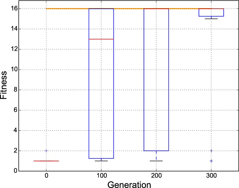
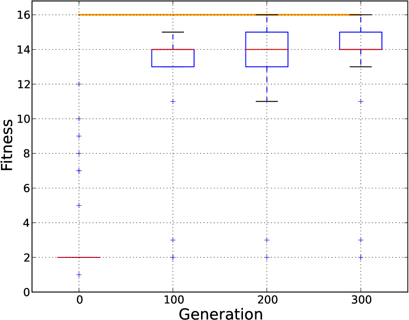
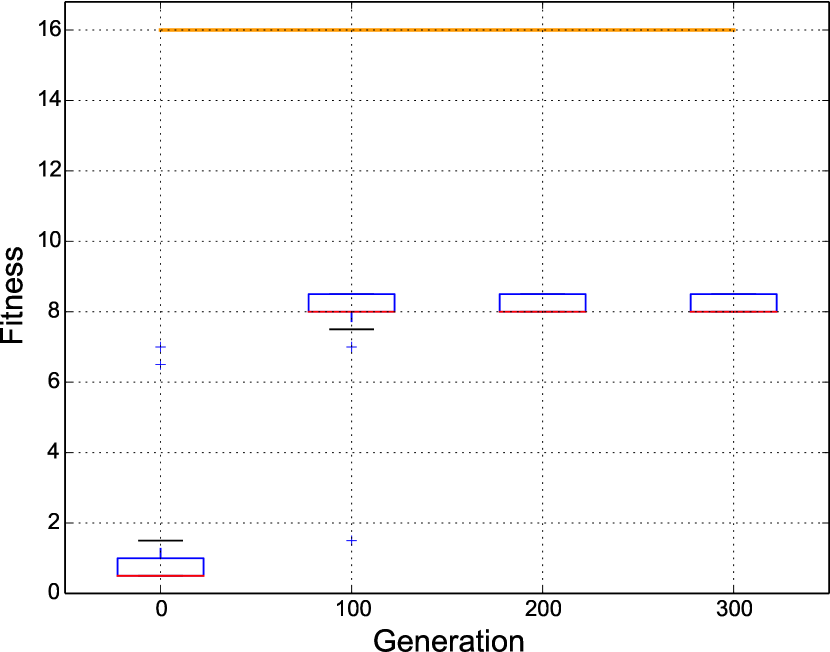
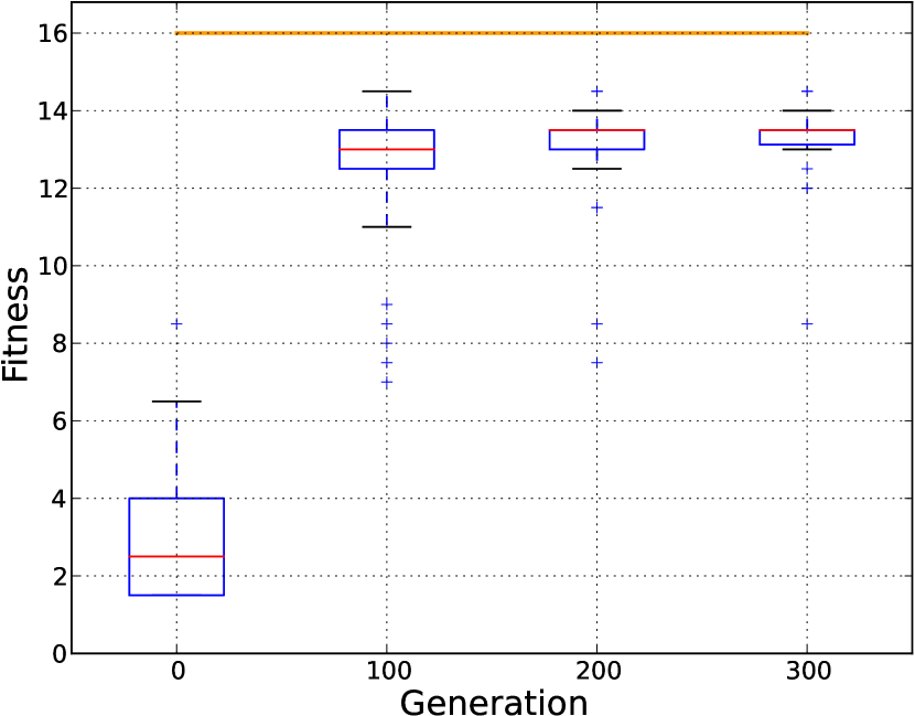
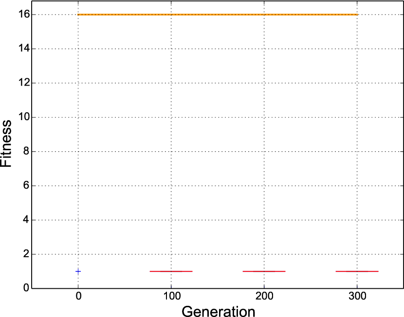
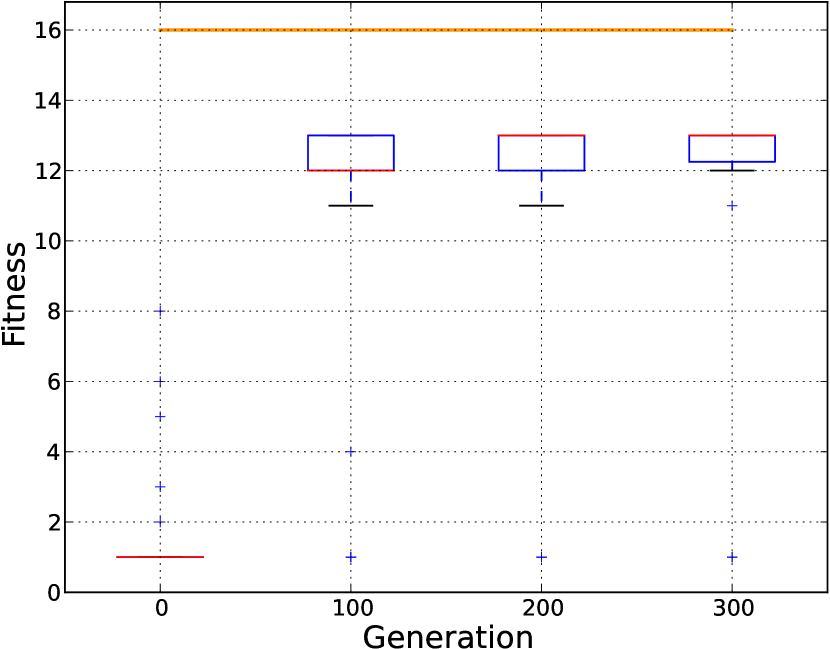
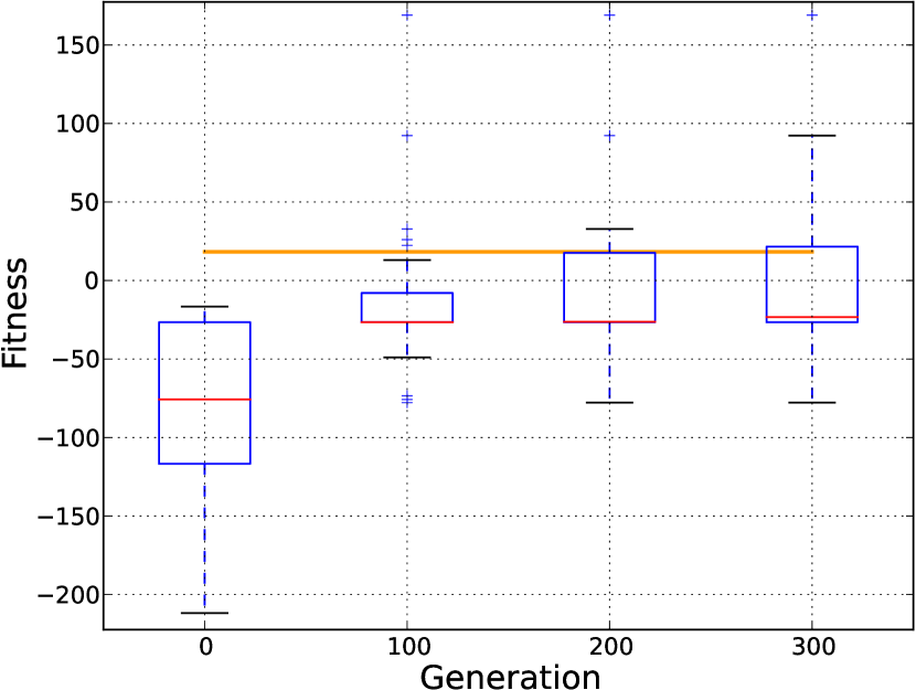
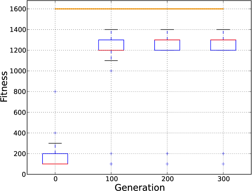
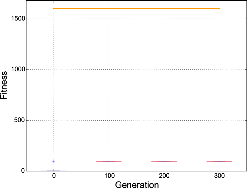
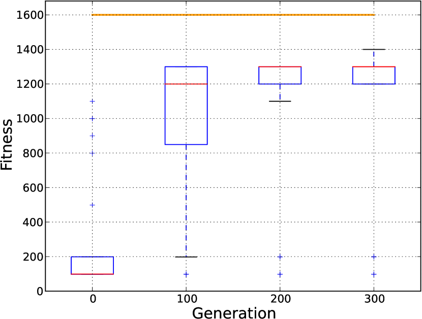
We evaluated two methods of associating a fitness value to each genome from these two evaluations: First, we calculated the arithmetic mean value of both runs and, as a second variant, we took the minimum value of both runs. In consequence, a good genome had to perform well in both environments, in the “minimum”-fitness function the selection was even harsher then in the “mean” variant. We found that the “minimum” variant of selection showed the higher selection pressure on evolving reactive control (compare Fig. 5 and Fig. 6): With the minimum-fitness regime the controllers had it harder to gather high fitness values, as they had to perform well in both environments, preventing evolution from “just considering on one of the two environments". We hoped that this would support the evolution of reactive control. As Fig. 6 to Fig. 6 show, it still did not produce the desired reactive Wankelmut behavior in the long run. Based on those findings, we used the double-environment evaluation with a minimum-of-both-run fitness function for all further quantitative analysis in this study, in order to maximize the selection pressure towards reactivity of the evolved controller.
II.2 Cumulative fitness regime
In another attempt to help the evolutionary algorithm to develop good reactive controllers we decided to reward genomes purely with cumulative fitness. The idea behind this was that every single step in the correct direction would be paying off in evolution. We assumed that, on the one hand, bootstrapping problems are minimized this way and, on the other hand, early reactive turns into the correct directions are rewarded even if they do not reach the switching threshold places initially. In this scenario, the fitness was computed by the Cumulative fitness regime described as
We found that the idea of cumulative fitness for every step was exceptionally bad. To our surprise both controller types managed to even outperform significantly the hand-coded “optimal” controller (see Fig. 7 and Fig. 7). Looking at the trajectories revealed that the evolutionary algorithm had found a “cheap trick” to maximize this purely cumulative fitness function without evolving the desired task: The controllers approached the threshold areas, thus gained the maximum reward without having to switch the behavior. They kept this place for the rest of the run. This cheap trick was found for both controllers, ANNs (see Fig. 7 and Fig. 7) and also by CTRNNs (see Fig. 7 and Fig. 7) in a less effective way. In both cases they actively avoided to behave like the desired reactive Wankelmut controller by avoiding to cross the threshold places.
II.3 Instant+Switch fitness regime
In order to prevent the “cheap trick” deadlock for evolution we discovered in the previous section, we again revised our fitness function to the Instant+Switch reward setting: We again rewarded for every correct switch the agent performed and, instead of a cumulative reward every time step, we rewarded the final (one instant) position of the agent. This way, bootstrapping problems could also be mediated as again movement in the right direction without reaching the threshold place for switching the behavior would be rewarded but it did not pay out to keep the position just before triggering the switch.The fitness function used here can be described as .
The highest fitness values in this setting were achieved by a CTRNNs (see Fig. 8). However this was again achieved by just quickly zig-zagging across the world without reacting to the environmental situation: The agents started off into the wrong direction (see Fig. 8 and Fig. 8) in one environmental setting. Evolved ANNs did not at all develop highly rewarded behaviors in this setting (see Fig. 8). However the best ANN genome evolved in principle parts of the desired behaviors for the first period of time: They started off in both environments into the correct direction and executed the behavioral switch one time but never closed the cycle back again (see Fig. 8 and Fig. 8). Overall, the desired reactive Wankelmut behavior was never fully evolved in neither one of the controller types.
II.4 Cumulative+Switch fitness regime
In a final attempt to achieve the desired behavior we also tested the Cumulative+Switch fitness regime where the controller was rewarded cumulatively for positioning of the agent over time as well as significant rewards for the correct switches were given. The fitness function can be described as .
Introducing the additional rewarding for correct switches prevented the evolutionary algorithm from falling into the “cheap trick” local optimum it did when it was only rewarded cumulatively per step. The results were almost similar to the ones obtained from the previous Instant+Switch regime: CTRNNs did not evolve anything close to the desired reactive Wankelmut behavior (see Fig. 9) and ANNs evolved again the first switching of behaviors but failed to evolve the switch back. (see Fig. 9 and Fig. 9). CTRNNs achieved again some significant reward by oscillating in both environments in a non-reactive oscillatory behavior (see Fig. 9 and Fig. 9), like they have evolved already in most of the other evolution regimes.
In another attempt to enforce reactivity of the evolved controller and considering the evolved solutions shown above, we tried to push the evolution towards more reactivity of the controllers. Thus, the evolutionary experiment was repeated with only 56 time-steps per evaluation (see Fig. 10). Again, CTRNNs evolved a higher fitness (Fig. 10) than ANNs (Fig. 10). However, this was still achieved with non-reactive fast oscillations (see Fig. 10 and Fig. 10). The ANN evolved into a behavior that oscillated in one environment although starting in the wrong direction initially (see Fig. 10. In the second environment, the best agent progressed very slowly towards the threshold place and no switch back was observed there Fig. 10).
The resulting controllers were also tested in a post-evaluation to check for reactive behaviors. This was done with a different environment that had maximum quality in the middle and two minima, one at the left end and one at the right end. Agents were tested in two evaluations with one initially positioning the robot at the left end and the second one with initially positioning the robot at the right end. While some controllers managed to operate reasonably in one of the two evaluations (oscillating between the initial position and the middle place), none of them did so for both starting places. Hence, we conclude that also in this experiment we did not see the correct controller that solves the Wankelmut task in a reactive way.
III Evolving a Hand-coded Network
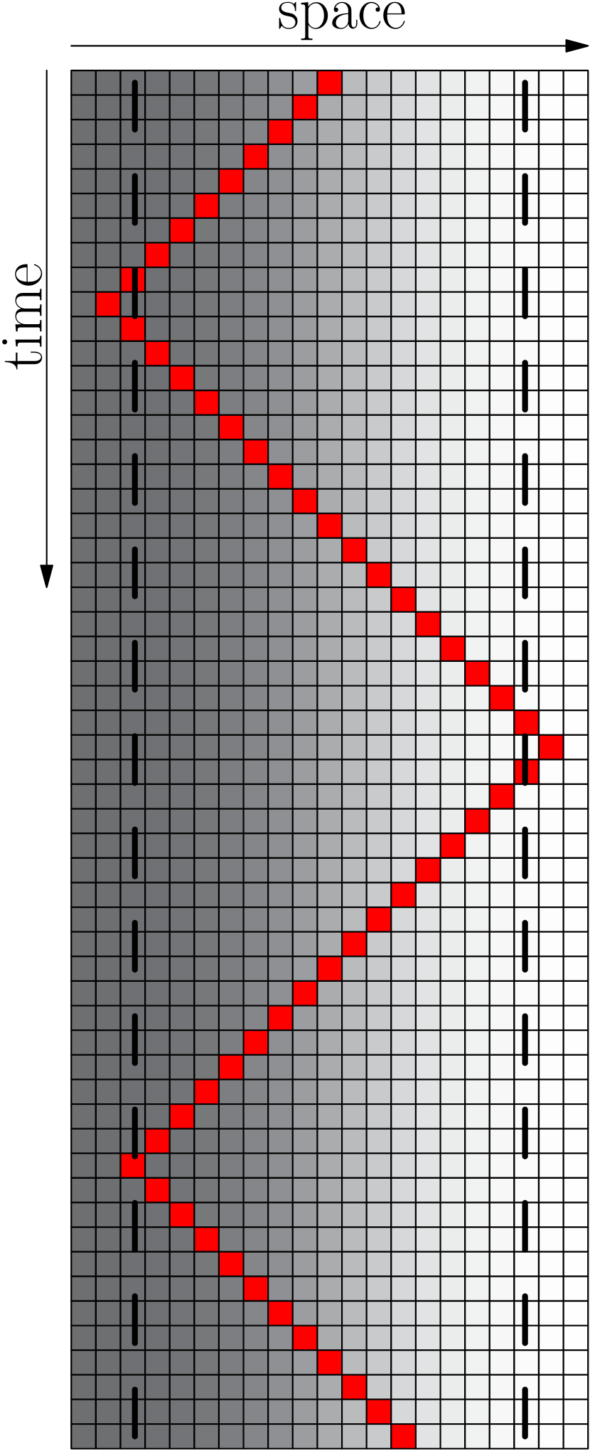
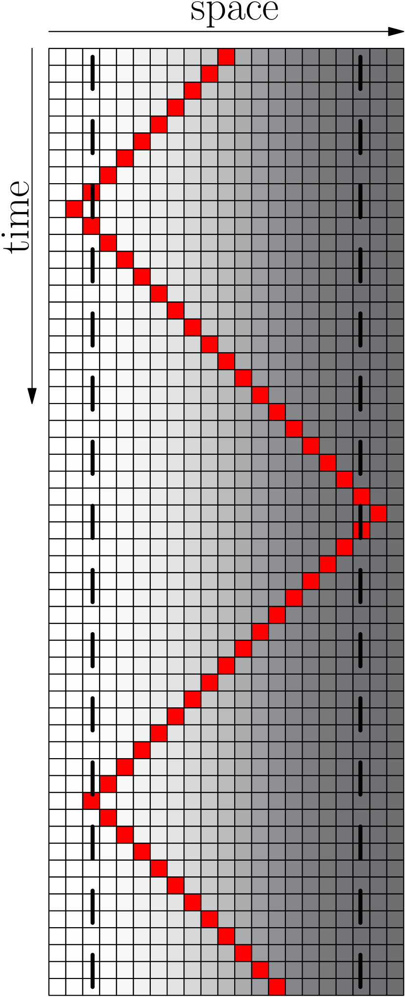
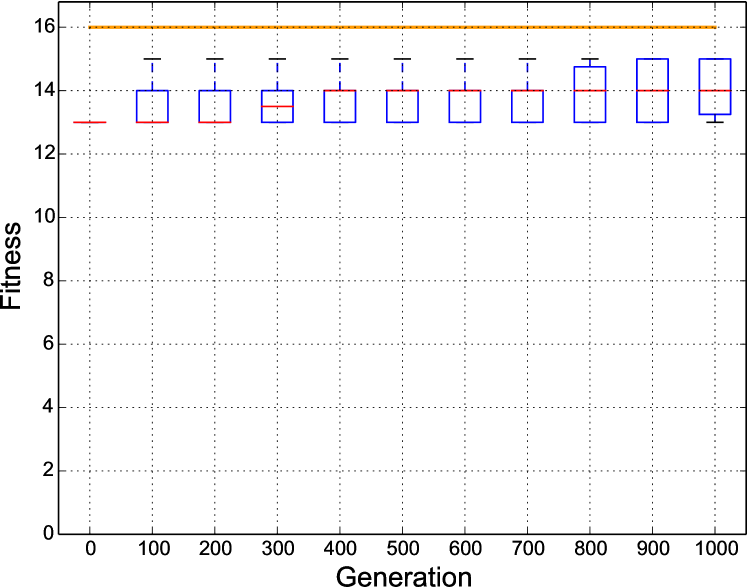
One of the hand-coded ANNs along with its behavior in the two environments is represented in Fig. 11 - 11. Although the agent is reactive and switches after passing the thresholds in each side, the behavior is not optimal: the agent had a delay in switching when it passes the thresholds at the environment represented in Fig. 11. In an attempt to get a perfect behavior, we initialized an ANN described in section I with the weights of the hand-coded ANN and used the fitness functions to evolve the network. Fig. 12 - 15 represent the results of the evolution for our different fitness regimes. Fig. 11 - 11 represent the best evolved network and its behaviors in both environments. As it is shown in the figures, evolution has flattened the network by giving values to additional links between the nodes and consequently, the evolved ANN demonstrates an optimal behavior.
VI Discussion and Conclusion
We have proposed the Wankelmut task which is a very simple task. In the Wankelmut task, we evolve a controller that switches between two alternative conflicting tasks. Yet, there is no prioritizing between the two subtasks and therefore it is not of the type of a subsumption architecture. It is also not repeatedly alternating between two subtasks since the switching between the two tasks is based on the environmental clues. The simplicity of the pseudo-code shown in Fig. 2 clearly demonstrates the simplicity of the required controller that implements an optimal, flexible, and reactive Wankelmut agent.
Our results indicate that plain-vanilla evolving ANNs easily can evolve the reactive uphill walk (see Fig. 4). However switching to the opposite behavior (downhill motion) and then flipping back was not found by any of our approaches, regardless what fitness regime we used and regardless what substrate we used for evolution (ANN or CTRNN). In all tested fitness regimes the desired behavior did not evolve. In one of these fitness regimes (Cummulative regime) evolution found a “cheap trick” to maximize the fitness with a surprising behavior, however, the desired reactive Wankelmut behavior did not evolve there.
In order to prove that the task is solvable by the encoding that we have used here, we designed two hand-coded ANNs that solve the task. However, the hand-coded networks demonstrated a behavior that is quite good but not optimal. To further improve this, we then evolved one of the hand-coded ANNs and achieved the optimal behavior showing that the encoding covers the solution and the evolution can evolve the behavior when it is searching in the vicinity of the solution (Fig.11).
We speculate that learning the downhill behavior “destroys” the already learned network structure for performing the uphill walk behavior. Thus, to evolve a combination of both would require a specific evolutionary framework that is designed to generate modules, store (freeze) useful modules and to combine them. However, such a functionality seems not to evolve from itself in our system in an emergent way.
Given that the hand-coded solution is very simple, a tree-based approach with exhaustive search or a genetic programming (GP) approach [30] is expected to be able to find the desired behavior. However we would expect also here to hit the same "wall of complexity", as controllers that require a bit more complexity overwhelm the exhaustive tree-search, while the existing local optima, that already fooled the ANN+Evo approach and the CTRNN+Evo approach, will also fool the stochastic GP search in a similar way. This remains to be tested in future experiments.
We point out that the target of evolving controllers for the Wankelmut task from scratch requires to evolve a behavioral switch. However, evolution of such a switch represents a hen-egg problem. The switch is useless without the two motion-modules (subnets) for uphill and downhill motion, while those sub-modules are useless without the switch.
In addition, we want to stress the fact that a similar behavior could be exerted by just switching the environment in an oscillatory way. This is not the same as our envisioned Wankelmut behavior, as our behavior is intrinsically switching its behavioral pattern in reaction to a stable environment. So it is intrinsic dynamics exhibited in a global stable environment and not a fixed (stable) behavioral pattern in a globally dynamic environment.
The Wankelmut task might also prove to be an interesting benchmark for more sophisticated methods that push towards modularization. Examples are Artificial Epigenetic Networks as reported by [31]: They used the coupled inverted pendulums benchmark [32] which requires the concurrent evolution of several behaviors similar to the Wankelmut task. However, the control of coupled inverted pendulums is more complex than the simple world of Wankelmut. Other methods alternate between different tasks on evolutionary time-scales [18] and there are methods that, in addition, also impose costs on connections between nodes in neural networks [19]. Other interesting approaches either pre-determine or push towards modularity [15]. The approach of HyperNEAT was tested for its capability to generate modular networks with a negative result in the sense that modularity was not automatically generated [33]. [34] reports modularity by imposing different selection pressures to different parts of the network.
In fact we propose here two challenges for the scientific community at once:
-
1.
The first challenge is to find the most simple uninformed evolutionary computation algorithm that can solve the Wankelmut task presented here. Then the community can search for the next simple task that shows to be unsolvable for this new algorithm. This will yield iterative progress in the field.
-
2.
The Wankelmut task is the simplest task found so far (concerning required memory size, number of modules, dimensionality of the world it operates in, etc.). Still, there might be even simpler tasks that already break plain-vanilla uninformed evolutionary computation, so we also pose the challenge to search for such simpler benchmark tasks.
It should be noted that there is no evidence that such walls of complexity are consistent in a way that breaking one wall may cause a new wall at a different position. This is quite similar to the reasoning behind the “no free lunch” theorem. Theoretically, an optimization algorithm cannot be optimal for all tasks. However, neither natural nor artificial evolution achieve in general optimal solutions. Instead, especially natural, evolution has proven to be a great heuristic for which the walls might be fixed in a certain place but definitely far away from the wall for state-of-the-art artificial evolution. Hence, we should try to search for that one heuristic that allows us to push all walls of many different tasks as far as possible forward (while still accepting the implications of no free lunch).
We think that either dismissing all pre-informed methods or finding minimally pre-informed methods to solve the Wankelmut task is important. Natural evolution has produced billions of billions of reactive and adaptive behaviors of organisms much more complex than the Wankelmut task and it has achieved this without any information that promoted self-complexification and self-modularization. In contrast, the evolutionary process started from scratch and developed all of that due to evolution-intrinsic forces. We think that this can be a lesson for evolutionary computation: studying how an uninformed process that is neither pre-fabricated towards complexification or modularization and which is not specifically rewarded for complexification or modularization can still yield complex solutions. Nature has shown it and evolutionary computation and biologists together should find out how this was achieved. Maybe this would then be not “evolutionary computation" anymore but rather “artificial evolution" a real valid, yet still simple model of natural evolution.
Author Contributions
T.S., P.Z., H.H. contributed to the writing of the paper in equal parts. T.S. had the initial idea of the problem study, defined the main problem statement, programmed the initial cellular simulator used in this study, and produced the schematic drawing (Fig. 1). P.Z. programmed the CTRNN code, hand-coded ANNs, parts of the analysis scripts, and scripts for the box plots. H.H. programmed the ANN code and the evolutionary code, parts of the analysis scripts, and the ‘asymptote’ script used to produce the trajectory figures. The numerical analysis and interpretation of results was a joint effort of all authors.
Funding
T.S. was supported by the EU FP7-FET PROACTIVE grant #601074 (ASSISIbf). P.Z. and H.H. were supported by the EU H2020-FET PROACTIVE grant #640959 (flora robotica).
Acknowledgments
We thank Dr. Jürgen Stradner for his early investigations of the problem (data not used here) and Dr. Ronald Thenius for his input of Artificial Neural Networks.
References
- [1] Richard S. Sutton and Andrew G. Barto. Reinforcement Learning: An Introduction. MIT Press, Cambridge, MA, USA, 1998.
- [2] Josh C. Bongard. Evolutionary robotics. Communications of the ACM, 56(8):74–83, 2013.
- [3] Mikhail Prokopenko. Grand challenges for computational intelligence. Frontiers in Robotics and AI, 1(2), 2014.
- [4] Agoston E. Eiben and Jim Smith. From evolutionary computation to the evolution of things. Nature, 521:476–482, 2015.
- [5] David H Wolpert and William G Macready. No free lunch theorems for optimization. Evolutionary Computation, IEEE Transactions on, 1(1):67–82, 1997.
- [6] Davide Marocco and Stefano Nolfi. Origins of communication in evolving robots. In From Animals to Animats 9: Proceedings of the Eighth International Conference on Simulation of Adaptive Behavior, volume 4095 of LNCS, pages 789–803. Springer-Verlag, 2006.
- [7] Stefano Nolfi and Dario Floreano. Evolutionary Robotics: The Biology, Intelligence, and Technology of Self-Organizing Machines. MIT Press, 2000.
- [8] Karl Sims. Evolving 3D morphology and behavior by competition. In R. Brooks and P. Maes, editors, Artificial Life IV, pages 28–39. MIT Press, 1994.
- [9] Jeff Clune, Benjamin E. Beckmann, Charles Ofria, and Robert T. Pennock. Evolving coordinated quadruped gaits with the HyperNEAT generative encoding. In Proceedings of the 2009 IEEE Congress on Evolutionary Computation (CEC), pages 2764–2771. IEEE, 2009.
- [10] P. Zahadat, D.J. Christensen, S.D. Katebi, and K. Stoy. Sensor-coupled fractal gene regulatory networks for locomotion control of a modular snake robot. In Proc. the 10th Int. Symposium on Distributed Autonomous Robotic Systems, pages 517–530, 2010.
- [11] Heiko Hamann, Jürgen Stradner, Thomas Schmickl, and Karl Crailsheim. A hormone-based controller for evolutionary multi-modular robotics: From single modules to gait learning. In Proceedings of the IEEE Congress on Evolutionary Computation (CEC’10), pages 244–251, 2010.
- [12] Payam Zahadat, Thomas Schmickl, and Karl Crailsheim. Evolving reactive controller for a modular robot: Benefits of the property of state-switching in fractal gene regulatory networks. In Tom Ziemke, Christian Balkenius, and John Hallam, editors, From Animals to Animats 12, volume 7426 of Lecture Notes in Computer Science, pages 209–218. Springer Berlin Heidelberg, 2012.
- [13] Dario Floreano and Laurent Keller. Evolution of adaptive behaviour in robots by means of darwinian selection. PLoS Biol, 8(1):1–8, 01 2010.
- [14] Hod Lipson. Principles of modularity, regularity, and hierarchy for scalable systems. In In GECCO Workshop on Modularity, Regularity, and Hierarchy in Evolutionary Computation, pages 125–128, 2004.
- [15] Stefano Nolfi. Using emergent modularity to develop control systems for mobile robots. Adaptive Behavior, 5:343–363, 1996.
- [16] Joseba Urzelai, Dario Floreano, Marco Dorigo, and Marco Colombetti. Incremental robot shaping. Connection Science, 10(3-4):341–360, 1998.
- [17] Richard J. Duro, José Antonio Becerra, and J. Santos. Behavior reuse and virtual sensors in the evolution of complex behavior architectures. Theory in Biosciences, 120(3-4):188–206, 2001.
- [18] Nadav Kashtan and Uri Alon. Spontaneous evolution of modularity and network motifs. Proc. Natl. Acad. Sci. U. S. A., 102(39):13773–13778, 2005.
- [19] Jeff Clune, Jean-Baptiste Mouret, and Hod Lipson. The evolutionary origins of modularity. Proceedings of the Royal Society B, 280(1755):20122863, 2013.
- [20] T. Shallice. From Neuropsychology to Mental Structure. Cambridge U. Press, 1988.
- [21] Valentino Braitenberg. Vehicles: experiments in synthetic psychology. MIT Press, Cambridge, MA, 1984.
- [22] John H. Holland. Adaptation in Natural and Artificial Systems. Univ. Michigan Press, Ann Arbor, MI, 1975.
- [23] Ingo Rechenberg. Evolutionsstrategie. Optimierung technischer Systeme nach Prinzipien der biologischen Evolution. Frommann Holzboog, 1973.
- [24] Charles Darwin. On the Origin of Species By Means of Natural Selection. John Murray, London, 1859.
- [25] Thomas Dyer Seeley. The wisdom of the hive: the social physiology of honey bee colonies. Havard University Press, Cambridge, Massachusetts, London, England, 1995.
- [26] Scott Camazine, Jean-Louis Deneubourg, Nigel R. Franks, James Sneyd, Guy Theraulaz, and Eric Bonabeau. Self-Organizing Biological Systems. Princeton Univ. Press, 2001.
- [27] Ken Ichi Funahashi and Yuichi Nakamura. Approximation of dynamical systems by continuous time recurrent neural networks. Neural Networks, 6(6):801–806, 1993.
- [28] Randall D. Beer. Parameter space structure of continuous-time recurrent neural networks. Neural Comput., 18(12):3009–3051, December 2006.
- [29] Andrew L. Nelson, Gregory J. Barlow, and Lefteris Doitsidis. Fitness functions in evolutionary robotics: A survey and analysis. Robotics and Autonomous Systems, 57:345–370, 2009.
- [30] John R. Koza. Genetic Programming: On the Programming of Computers by Means of Natural Selection. MIT Press, 1992.
- [31] A. P. Turner, L. S. D. Caves, S. Stepney, A. M. Tyrrell, and M. A. Lones. Artificial epigenetic networks: Automatic decomposition of dynamical control tasks using topological self-modification. IEEE Transactions on Neural Networks and Learning Systems, 2016.
- [32] Heiko Hamann, Thomas Schmickl, and Karl Crailsheim. Coupled inverted pendulums: A benchmark for evolving decentral controllers in modular robotics. In Natalio Krasnogor and Pier Luca Lanzi, editors, Proceedings of the 13th Annual Genetic and Evolutionary Computation Conference, GECCO 2011, pages 195–202. ACM, 2011.
- [33] Jeff Clune, Benjamin E. Beckmann, Philip K. McKinley, and Charles Ofria. Investigating whether hyperNEAT produces modular neural networks. In GECCO, pages 635–642, 2010.
- [34] Josh C. Bongard. Spontaneous evolution of structural modularity in robot neural network controllers: artificial life/robotics/evolvable hardware. In Proceedings of the 13th annual conference on Genetic and evolutionary computation, GECCO ’11, pages 251–258, New York, NY, USA, 2011. ACM.
Figures