Performance Impact of Idle Mode Capability on Dense Small Cell Networks

Abstract

Very recent studies showed that in a fully loaded dense small cell network (SCN), the coverage probability performance will continuously decrease with the network densification. Such new results were captured in IEEE ComSoc Technology News with an alarming title of “Will Densification Be the Death of 5G?”. In this paper, we revisit this issue from more practical views of realistic network deployment, such as a finite number of active base stations (BSs) and user equipments (UEs), a decreasing BS transmission power with the network densification, and so on. Particularly, in dense SCNs, due to an oversupply of BSs with respect to UEs, a large number of BSs can be put into idle modes without signal transmission, if there is no active UE within their coverage areas. Setting those BSs into idle modes mitigates unnecessary inter-cell interference and reduces energy consumption. In this paper, we investigate the performance impact of such BS idle mode capability (IMC) on dense SCNs. Different from existing work, we consider a realistic path loss model incorporating both line-of-sight (LoS) and non-line-of-sight (NLoS) transmissions. Moreover, we obtain analytical results for the coverage probability, the area spectral efficiency (ASE) and the energy efficiency (EE) performance for SCNs with the BS IMC and show that the performance impact of the IMC on dense SCNs is significant. As the BS density surpasses the UE density in dense SCNs, the coverage probability will continuously increase toward one, addressing previous concerns on “the death of 5G”. Finally, the performance improvement in terms of the EE performance is also investigated for dense SCNs using practical energy models developed in the Green-Touch project.

I Introduction

Dense small cell networks (SCNs), comprised of remote radio heads, metrocells, picocells, femtocells, relay nodes, etc., have attracted significant attention as one of the most promising approaches to rapidly increase network capacity and meet the ever-increasing data traffic demands [1]. Indeed, the orthogonal deployment of dense SCNs within the existing macrocell networks [2], i.e., small cells and macrocells operating on different frequency spectrum (Small Cell Scenario #2a [2]), has been selected as the workhorse for capacity enhancement in the 4th-generation (4G) and the 5th-generation (5G) networks, developed by the 3rd Generation Partnership Project (3GPP) [3]. In this paper, we focus on the analysis of these dense SCNs with an orthogonal deployment in the existing macrocell networks.

In the seminal work of Andrews, Baccelli, and Ganti [4], a conclusion was reached: the density of base stations (BSs) would not affect the coverage probability performance in interference-limited and fully-loaded wireless networks, where the coverage probability is defined as the probability that the signal-to-interference-plus-noise ratio (SINR) of a typical user equipment (UE) is above a SINR threshold $\gamma$. Consequently, the area spectral efficiency (ASE) performance in $\textrm{bps/Hz/km}^{2}$ would scale linearly with the network densification [4], which forecasts a bright future for dense SCNs in 4G and 5G. The intuition of such conclusion is that the increase in the interference power caused by a denser network would be exactly compensated by the increase in the signal power due to the reduced distance between transmitters and receivers. This coverage probability behavior predicted in [4] is shown in Fig. 1.

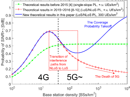
Fig. 1: Theoretical performance comparison of the coverage probability when the SINR threshold $\gamma=0$ dB. Note that all the results are obtained using practical 3GPP channel models [6, 7], which will be introduced in details later. Moreover, the BS density regions for the 4G and 5G networks have been illustrated in the figure, considering that the typical BS density of the 4G SCNs is in the order of tens of $\textrm{BSs/km}^{2}$ [2, 3].

However, it is important to note that such conclusion was obtained with considerable simplifications on the network condition and propagation environment. For example, all BSs were assumed to be active and a single-slop path loss model was used. It would be interesting to investigate whether the conclusion still holds in real-world environment featuring more complicated BS behaviors and radio propagation environment.

To this end, a few noteworthy studies have been carried out recently to revisit the network performance analysis of dense SCNs using more practical propagation models. In [8], the authors considered a multi-slope piece-wise path loss function, while in [9], the authors modeled line-of-sight (LoS) and non-line-of-sight (NLoS) transmissions as probabilistic events for a millimeter wave communication scenario. In our recent work [10], we further considered both piece-wise path loss functions and probabilistic LoS and NLoS transmissions. The above new studies demonstrated that when the BS density is larger than a threshold $\lambda^{*}$, the coverage probability will continuously decrease as the SCN becomes denser. The intuition behind such result is that the interference power increases faster than the signal power in dense SCNs due to the transition of a large number of interference paths from NLoS (usually with a large path loss exponent) to LoS (usually with a small path loss exponent). Such new results were later captured in IEEE ComSoc Technology News with an alarming title of “Will Densification Be the Death of 5G?” [11]. Fig. 1 shows the coverage probability result in [8, 9, 10], where $\lambda^{*}$ is around 20 $\textrm{BSs/km}^{2}$. The key message is that, when deploying dense SCNs, an increased BS density may lead to worse network performance, and hence the future of 5G is shrouded in darkness.

In this paper, we will take another look at “the death of 5G” from more practical views of realistic network deployment, such as a finite number of active BSs and UEs, a decreasing BS transmission power with the network densification, and so on. Particularly, since the UE density is finite in practical networks, a large number of BSs in dense SCNs could switch off their transmission modules and thus enter idle modes, if there is no active UE within their coverage areas. Setting those BSs to idle modes can mitigate unnecessary inter-cell interference and reduce energy consumption [5, 12, 13, 14]. In other words, by dynamically muting idle BSs, the interference suffered by UEs from always-on control channels, e.g., synchronization and broadcast channels, and data channels can be reduced, thus improving UEs’ coverage probability. This idle mode feature at BSs is referred to as the idle mode capability (IMC) hereafter. Furthermore, the energy efficiency (EE) of SCNs with the IMC can be significantly enhanced because (i) BSs without any active UE can be temporarily put into idle modes with low energy consumption, and (ii) every active BS usually benefits from high-SINR and thus energy-efficient links with its associated UEs due to the BS diversity gain [5], i.e., each UE selects the serving BS with the highest SINR from a surplus of BSs in dense SCNs. It is very important to note that a BS in idle mode may still consume a non-negligible amount of energy, thus impacting the EE of SCNs. In this paper, we use a practical power model developed in the Green-Touch project [15] to evaluate the EE performance in realistic scenarios. Such power model will be formally introduced later.

In this paper, we investigate for the first time the performance impact of the IMC on dense SCNs considering LoS and NLoS transmissions. As an example to demonstrate such impact, our results with a UE density of $300\thinspace\textrm{UEs/km}^{2}$ (a typical UE density in 5G [3]) are compared with the existing results in Fig. 1. The performance impact of the IMC on the coverage probability is shown to be significant. As the BS density surpasses the UE density in future dense and ultra-dense SCNs [3], thus creating a surplus of BSs, the coverage probability will continuously increase toward one, addressing the critical issue of coverage probability decrease that may cause “the death of 5G” shown in Fig. 1. Such performance behavior of the coverage probability increasing toward one in dense SCNs, is referred to as the Coverage Probability Takeoff hereafter. The intuition behind the Coverage Probability Takeoff is that beyond a certain BS density threshold, the interference power will be less than that of the case with all BSs being active thanks to the BS IMC, plus the signal power will continuously rise due to the BS diversity gain, thus leading to a better SINR performance as the network evolves into a dense one.

Compared with existing work, the main contributions of this paper are:

• Analytical results are obtained for the coverage probability and the ASE performance of SCNs with the BS IMC using a general path loss model incorporating both LoS and NLoS transmissions. Note that existing work on the IMC only treated a single-slope path loss model, where a UE is always associated with its nearest BS [5, 13], while our work considers more practical path loss models with probabilistic LoS and NLoS transmissions, where UEs may connect to a farther BS with a LoS path.

• A lower bound, an upper bound and an approximate expression of the active BS density are derived for SCNs with the IMC, considering practical path loss models with probabilistic LoS and NLoS transmissions.

• The performance improvement in terms of the EE is also investigated for dense SCNs using practical energy models developed in the Green-Touch project [15] and practical 3GPP propagation models with Rician fading, correlated shadow fading, etc.

The rest of this paper is structured as follows. Section II provides a brief review of related work. Section III describes the system model featuring the BS IMC. Section IV presents our theoretical results on the coverage probability, the ASE, the EE and the active BS density, with their applications in two 3GPP special cases. The numerical results are discussed in Section V, with remarks shedding new light on the issue of “the death of 5G”. The conclusions are drawn in Section VI.

II Related Work

In stochastic geometry, BS positions are typically modeled as a Homogeneous Poisson Point Process (HPPP) on the plane, and closed-form expressions of coverage probability can be found for some scenarios in single-tier cellular networks [4] and multi-tier cellular networks [17]. The major conclusion in [4, 17] is that neither the number of cells nor the number of cell tiers changes the coverage probability in interference-limited fully-loaded wireless networks.

Recently, a few noteworthy studies have been carried out to further investigate the network performance analysis for dense and ultra-dense SCNs under more practical propagation models. As discussed in Section I, the authors of [8, 9, 10] found that the coverage probability performance will start to decrease when the BS density is sufficiently large. The intuition behind this result is that as the BS density becomes larger than a threshold, the interference power increases faster than the signal power due to the transition of a large number of interference paths from NLoS to LoS.

However, all of the above work did not consider an important factor: as the BS density increases, a large number of BSs can be put into idle mode without signal transmission, if there is no active UE within their coverage areas. This is a new network behavior arising from the surplus of BSs with respect to UEs, i.e., it may happen that a significant number of BSs may not have any active UE in their coverage areas during certain time periods. Therefore, such BSs could mute their transmission to mitigate unnecessary inter-cell interference and reduce energy consumption [5, 12, 13, 18, 14].

Up to now, the limited existing work that did consider the IMC, only treated a simplistic single-slope path loss model for homogeneous SCNs [5, 12, 13, 18] or for the co-channel deployment of heterogeneous networks [14]. Such path loss assumption is not practical for realistic SCNs and may yield misleading conclusions reading the network performance, as addressed in [8, 9, 10].

Motivated by the above observations, in this paper, we investigate for the first time the performance impact of the IMC on dense SCNs considering probabilistic LoS and NLoS transmissions. Note that compared with our previous work that also considered probabilistic LoS and NLoS transmissions [10], this paper present new contributions as follows,

• Our previous work [10] corroborates “the death of 5G” [11] by considering probabilistic LoS and NLoS transmissions and an infinite number of UEs in the network. However, in this work, we present new theoretical results that can mitigate “the death of 5G” by considering a finite number of UEs exploited by the BS IMC.

• The new theoretical work in this paper compared with [10] is that a lower bound, an upper bound and an approximate expression of the active BS density are derived for SCNs with the IMC, considering practical path loss models with probabilistic LoS and NLoS transmissions.

• Moreover, compared with [10], the performance improvement in terms of the EE is also investigated in this paper.

III System Model

We consider a downlink (DL) cellular network with BSs deployed on a plane according to a homogeneous Poisson point process (HPPP) $\Phi$ with a density of $\lambda$ $\textrm{BSs/km}^{2}$. Active UEs are Poisson distributed in the considered DL network with a density of $\rho$ $\textrm{UEs/km}^{2}$. Here, we only consider active UEs in the network because non-active UEs do not trigger data transmission, and thus they are ignored in our analysis. Note that the total UE number in cellular networks should be much higher than the number of the active UEs, but at a certain time slot and on a certain frequency band, the active UEs with data traffic demands are not too many. As discussed in Section I, a typical density of the active UEs in 5G should be around $300\thinspace\textrm{UEs/km}^{2}$ [3].

In our previous work [10, 19] and other related work [8, 9], $\rho$ was assumed to be infinite or considerably larger than $\lambda$ so that each BS has at least one associated UE in its coverage. In this work, we impose no such constraint on $\rho$, and hence a BS with the IMC will enter an idle mode if there is no UE connected to it, which reduces interference to neighboring UEs as well as energy consumption of the network. Since UEs are randomly and uniformly distributed in the network, we assume that the active BSs also follow an HPPP distribution $\tilde{\Phi}$ [5, 12, 13, 18], the density of which is denoted by $\tilde{\lambda}$ $\textrm{BSs/km}^{2}$. Note that $\tilde{\lambda}\leq\lambda$, and $\tilde{\lambda}\leq\rho$ since one UE is served by at most one BS. Obviously, a larger $\rho$ requires more active BSs with a larger $\tilde{\lambda}$ to serve the active UEs.

It is very important to note that, up to now, there is no theoretical proof showing that the active BSs should follow an HPPP since the activation of each BS depends on the UE distribution in its vicinity. Having said that, the HPPP assumption has been widely used in the literature, such as [5, 12, 13, 18]. Indeed, later we will present simulation results backing up our theoretical findings based on the HPPP assumption, where the computational engines for the computer simulations and theoretical analyses follow different principles. More specifically, in our simulations, no assumption was made on the distribution of the active BSs. They are generated according to the UEs’ selection. In contrast, the HPPP assumption was only used to obtain the analytical results. This methodology has also been used in [5, 12, 13, 18]. The intuition of this conclusion is that since no clustering behavior of UEs and no correlation among UEs’ channels have been considered in the analysis, the activation and deactivation of each BS is uniformly and randomly distributed across the entire network, which leads to the HPPP assumption.

Following [19, 10], we adopt a very general path loss model, in which the path loss $\zeta\left(r\right)$ as a function of $r$ is segmented into $N$ pieces written as

$$\zeta\left(r\right)=\begin{cases}\zeta_{1}\left(r\right),&\textrm{when }0\leq r\leq d_{1}\\ \zeta_{2}\left(r\right),&\textrm{when }d_{1}<r\leq d_{2}\\ \vdots&\vdots\\ \zeta_{N}\left(r\right),&\textrm{when }r>d_{N-1}\end{cases},$$ (1)

where each piece $\zeta_{n}\left(r\right),n\in\left\{1,2,\ldots,N\right\}$ is modeled as

$$\zeta_{n}\left(r\right)=\begin{cases}\begin{array}[]{l}\zeta_{n}^{\textrm{L}}\left(r\right)=A_{n}^{{\rm{L}}}r^{-\alpha_{n}^{{\rm{L}}}},\\ \zeta_{n}^{\textrm{NL}}\left(r\right)=A_{n}^{{\rm{NL}}}r^{-\alpha_{n}^{{\rm{NL}}}},\end{array}&\begin{array}[]{l}\textrm{LoS Prob.:}\leavevmode\nobreak\ \textrm{Pr}_{n}^{\textrm{L}}\left(r\right)\\ \textrm{NLoS Prob.:}\leavevmode\nobreak\ 1-\textrm{Pr}_{n}^{\textrm{L}}\left(r\right)\end{array},\end{cases}$$ (2)

where

• $\zeta_{n}^{\textrm{L}}\left(r\right)$ and $\zeta_{n}^{\textrm{NL}}\left(r\right),n\in\left\{1,2,\ldots,N\right\}$ are the $n$-th piece path loss functions for the LoS transmission and the NLoS transmission, respectively,

• $A_{n}^{{\rm{L}}}$ and $A_{n}^{{\rm{NL}}}$ are the path losses at a reference distance $r=1$ for the LoS and the NLoS cases, respectively,

• $\alpha_{n}^{{\rm{L}}}$ and $\alpha_{n}^{{\rm{NL}}}$ are the path loss exponents for the LoS and the NLoS cases, respectively.

In practice, $A_{n}^{{\rm{L}}}$, $A_{n}^{{\rm{NL}}}$, $\alpha_{n}^{{\rm{L}}}$ and $\alpha_{n}^{{\rm{NL}}}$ are constants obtainable from field tests [6, 7].

Moreover, $\textrm{Pr}_{n}^{\textrm{L}}\left(r\right)$ is the $n$-th piece LoS probability function that a transmitter and a receiver separated by a distance $r$ has a LoS path, which is assumed to be a monotonically decreasing function with regard to $r$. Such assumption has been confirmed by existing measurement studies [6, 7]. For convenience, $\left\{\zeta_{n}^{\textrm{L}}\left(r\right)\right\}$ and $\left\{\zeta_{n}^{\textrm{NL}}\left(r\right)\right\}$ are further stacked into piece-wise functions written as

$$\zeta^{Path}\left(r\right)=\begin{cases}\zeta_{1}^{Path}\left(r\right),&\textrm{when }0\leq r\leq d_{1}\\ \zeta_{2}^{Path}\left(r\right),&\textrm{when }d_{1}<r\leq d_{2}\\ \vdots&\vdots\\ \zeta_{N}^{Path}\left(r\right),&\textrm{when }r>d_{N-1}\end{cases},$$ (3)

where the string variable $Path$ takes the value of “L” and “NL” for the LoS and the NLoS cases, respectively.

Besides, $\left\{\textrm{Pr}_{n}^{\textrm{L}}\left(r\right)\right\}$ is stacked into a piece-wise function as

$$\textrm{Pr}^{\textrm{L}}\left(r\right)=\begin{cases}\textrm{Pr}_{1}^{\textrm{L}}\left(r\right),&\textrm{when }0\leq r\leq d_{1}\\ \textrm{Pr}_{2}^{\textrm{L}}\left(r\right),&\textrm{when }d_{1}<r\leq d_{2}\\ \vdots&\vdots\\ \textrm{Pr}_{N}^{\textrm{L}}\left(r\right),&\textrm{when }r>d_{N-1}\end{cases}.$$ (4)

Note that the generality and the practicality of the adopted path loss model (1) have been well established in [10]. In more detail, this model is consistent with the ones adopted in the 3GPP [6], [7], and includes those models considered in [8] and [9] as its special cases.

In this paper, we assume a practical user association strategy (UAS), in which each UE is connected to the BS with the smallest path loss (i.e., with the largest $\zeta\left(r\right)$) to the UE [9, 10]. Note that in our previous work [19] and some other existing work, e.g., [4, 8], it was assumed that each UE should be associated with its closest BS. Such assumption is not appropriate for the considered path loss model in (1), because in practice a UE should connect to a BS offering the largest received signal strength. Such BS does not necessarily have to be the nearest one to the UE, and it could be a farther one with a strong LoS path.

Moreover, we assume that each BS/UE is equipped with an isotropic antenna, and that the multi-path fading between a BS and a UE is modeled as independently identical distributed (i.i.d.) Rayleigh fading [8, 9, 10]. Note that a practical 3GPP model with distance-dependent Rician fading [7] and correlated shadow fading [6] will also be considered and simulated in Section V to show their minor impact on our conclusions. More specifically,

• We adopt a practical Rician fading defined in the 3GPP [7], where the $K$ factor in dB scale (the ratio between the power in the direct path and the power in the other scattered paths) is modeled as $K[\textrm{dB}]=13-0.03r$, where $r$ is the distance in meter.

• We consider a practical correlated shadow fading defined in 3GPP [6], where the shadow fading in dB is modeled as zero-mean Gaussian random variables, e.g., with a standard deviation of 10 dB. The correlation coefficient between the shadow fading values associated with two different BSs is denoted by $\tau$, e.g., $\tau=0.5$ in [6].

IV Main Results

In this section, we study the performance of SCNs in terms of the coverage probability, the ASE and the EE by considering the performance of a typical UE located at the origin $o$.

IV-A The Coverage Probability

First, we investigate the coverage probability that the typical UE’s SINR is above a designated threshold $\gamma$:

$$p^{\textrm{cov}}\left(\lambda,\gamma\right)=\textrm{Pr}\left[\mathrm{SINR}>\gamma\right],$$ (5)

where the SINR is computed by

$$\mathrm{SINR}=\frac{P\zeta\left(r\right)h}{I_{\textrm{agg}}+P_{{\rm{N}}}}.$$ (6)

Here, $h$ is the channel gain, which is modeled as an exponentially distributed random variable (RV) with a mean of one (due to our consideration of Rayleigh fading mentioned above), $P$ and $P_{{\rm{N}}}$ are the BS transmission power and the additive white Gaussian noise (AWGN) power at each UE, respectively, and $I_{\textrm{agg}}$ is the cumulative interference given by

$$I_{\textrm{agg}}=\sum_{i:\,b_{i}\in\tilde{\Phi}\setminus b_{o}}P\beta_{i}g_{i},$$ (7)

where $b_{o}$ is the BS serving the typical UE, and $b_{i}$, $\beta_{i}$ and $g_{i}$ are the $i$-th interfering BS, the path loss from $b_{i}$ to the typical UE and the multi-path fading channel gain associated with $b_{i}$, respectively. Note that when all BSs are assumed to be active, the set of all BSs $\Phi$ should be used in the expression of $I_{\textrm{agg}}$ [8, 9, 10]. Here, in (7), only the active BSs in $\tilde{\Phi}\setminus b_{o}$ inject effective interference into the network, where $\tilde{\Phi}$ denotes the set of the active BSs. In other words, the BSs in idle modes are not taken into account in the analysis of $I_{\textrm{agg}}$.

Based on the path loss model in (1) and the adopted UAS, we present our result of $p^{\textrm{cov}}\left(\lambda,\gamma\right)$ in Theorem 1.

Theorem 1.

Considering the path loss model in (1) and the presented UAS, the probability of coverage $p^{{\rm{cov}}}\left(\lambda,\gamma\right)$ can be derived as

$$p^{{\rm{cov}}}\left(\lambda,\gamma\right)=\sum_{n=1}^{N}\left(T_{n}^{{\rm{L}}}+T_{n}^{{\rm{NL}}}\right),$$ (8)

where $T_{n}^{{\rm{L}}}=\int_{d_{n-1}}^{d_{n}}{\rm{Pr}}\left[\frac{P\zeta_{n}^{{\rm{L}}}\left(r\right)h}{I_{{\rm{agg}}}+P_{{\rm{N}}}}>\gamma\right]f_{R,n}^{{\rm{L}}}\left(r\right)dr$, $T_{n}^{{\rm{NL}}}=\int_{d_{n-1}}^{d_{n}}{\rm{Pr}}\left[\frac{P\zeta_{n}^{{\rm{NL}}}\left(r\right)h}{I_{{\rm{agg}}}+P_{{\rm{N}}}}>\gamma\right]f_{R,n}^{{\rm{NL}}}\left(r\right)dr$, and $d_{0}$ and $d_{N}$ are defined as $0$ and $+\infty$, respectively. Moreover, $f_{R,n}^{{\rm{L}}}\left(r\right)$ and $f_{R,n}^{{\rm{NL}}}\left(r\right)$ $\left(d_{n-1}<r\leq d_{n}\right)$, are represented by

$$f_{R,n}^{{\rm{L}}}\left(r\right)=\exp\left(-\int_{0}^{r_{1}}\left(1-{\rm{Pr}}^{{\rm{L}}}\left(u\right)\right)2\pi u\lambda du\right)\exp\left(-\int_{0}^{r}{\rm{Pr}}^{{\rm{L}}}\left(u\right)2\pi u\lambda du\right){\rm{Pr}}_{n}^{{\rm{L}}}\left(r\right)2\pi r\lambda,$$ (9)

and

$$f_{R,n}^{{\rm{NL}}}\left(r\right)=\exp\left(-\int_{0}^{r_{2}}{\rm{Pr}}^{{\rm{L}}}\left(u\right)2\pi u\lambda du\right)\exp\left(-\int_{0}^{r}\left(1-{\rm{Pr}}^{{\rm{L}}}\left(u\right)\right)2\pi u\lambda du\right)\left(1-{\rm{Pr}}_{n}^{{\rm{L}}}\left(r\right)\right)2\pi r\lambda,$$ (10)

where $r_{1}$ and $r_{2}$ are given implicitly by the following equations as

$$r_{1}=\underset{r_{1}}{\arg}\left\{\zeta^{{\rm{NL}}}\left(r_{1}\right)=\zeta_{n}^{{\rm{L}}}\left(r\right)\right\},$$ (11)

and

$$r_{2}=\underset{r_{2}}{\arg}\left\{\zeta^{{\rm{L}}}\left(r_{2}\right)=\zeta_{n}^{{\rm{NL}}}\left(r\right)\right\}.$$ (12)

In addition, ${\rm{Pr}}\left[\frac{P\zeta_{n}^{{\rm{L}}}\left(r\right)h}{I_{{\rm{agg}}}+P_{{\rm{N}}}}>\gamma\right]$ and ${\rm{Pr}}\left[\frac{P\zeta_{n}^{{\rm{NL}}}\left(r\right)h}{I_{{\rm{agg}}}+P_{{\rm{N}}}}>\gamma\right]$ are respectively computed by

$${\rm{Pr}}\left[\frac{P\zeta_{n}^{{\rm{L}}}\left(r\right)h}{I_{{\rm{agg}}}+P_{{\rm{N}}}}>\gamma\right]=\exp\left(-\frac{\gamma P_{{\rm{N}}}}{P\zeta_{n}^{{\rm{L}}}\left(r\right)}\right)\mathscr{L}_{I_{{\rm{agg}}}}^{{\rm{L}}}\left(\frac{\gamma}{P\zeta_{n}^{{\rm{L}}}\left(r\right)}\right),$$ (13)

where $\mathscr{L}_{I_{{\rm{agg}}}}^{{\rm{L}}}\left(s\right)$ is the Laplace transform of $I_{{\rm{agg}}}$ for LoS signal transmission evaluated at $s$, which can be further written as

$$\mathscr{L}_{I_{{\rm{agg}}}}^{{\rm{L}}}\left(s\right)=\exp\left(-2\pi\tilde{\lambda}\int_{r}^{+\infty}\frac{{\rm{Pr}}^{{\rm{L}}}\left(u\right)u}{1+\left(sP\zeta^{{\rm{L}}}\left(u\right)\right)^{-1}}du\right)\exp\left(-2\pi\tilde{\lambda}\int_{r_{1}}^{+\infty}\frac{\left[1-{\rm{Pr}}^{{\rm{L}}}\left(u\right)\right]u}{1+\left(sP\zeta^{{\rm{NL}}}\left(u\right)\right)^{-1}}du\right),$$ (14)

and

$${\rm{Pr}}\left[\frac{P\zeta_{n}^{{\rm{NL}}}\left(r\right)h}{I_{{\rm{agg}}}+P_{{\rm{N}}}}>\gamma\right]=\exp\left(-\frac{\gamma P_{{\rm{N}}}}{P\zeta_{n}^{{\rm{NL}}}\left(r\right)}\right)\mathscr{L}_{I_{{\rm{agg}}}}^{{\rm{NL}}}\left(\frac{\gamma}{P\zeta_{n}^{{\rm{NL}}}\left(r\right)}\right),$$ (15)

where $\mathscr{L}_{I_{{\rm{agg}}}}^{{\rm{NL}}}\left(s\right)$ is the Laplace transform of $I_{{\rm{agg}}}$ for NLoS signal transmission evaluated at $s$, which can be further written as

$$\mathscr{L}_{I_{{\rm{agg}}}}^{{\rm{NL}}}\left(s\right)=\exp\left(-2\pi\tilde{\lambda}\int_{r_{2}}^{+\infty}\frac{{\rm{Pr}}^{{\rm{L}}}\left(u\right)u}{1+\left(sP\zeta^{{\rm{L}}}\left(u\right)\right)^{-1}}du\right)\exp\left(-2\pi\tilde{\lambda}\int_{r}^{+\infty}\frac{\left[1-{\rm{Pr}}^{{\rm{L}}}\left(u\right)\right]u}{1+\left(sP\zeta^{{\rm{NL}}}\left(u\right)\right)^{-1}}du\right).$$ (16)

Proof:

The proof is very similar to that for Theorem 1 in [10]. Hence, we omit the proof here for brevity. The comparison between Theorem 1 in [10] and the proposed theorem will be explained in the sequel. ∎

From Theorem 1 and comparing it with the main result in [10], which was derived for the case with all BSs being active, it is important to note that:

• The impact of the serving BS selection on the coverage probability is measured by (9) and (10), the expressions of which are based on $\lambda$, not on $\tilde{\lambda}$. This is the same as Theorem 1 of [10].

• The impact of $I_{\textrm{agg}}$ on the coverage probability is measured by (14) and (16). Since only the active BSs emit effective interference into the considered SCN, the expressions of (14) and (16) are thus based on $\tilde{\lambda}$, not on $\lambda$. This is different from Theorem 1 of [10].

• The derivation of $\tilde{\lambda}$ is non-trivial, and it will be treated later in the following subsections.

Besides, from Theorem 1, we can draw an important intuition summarized in Lemma 2.

Lemma 2.

$p^{\textrm{cov}}\left(\lambda,\gamma\right)$ with the BS IMC is larger than that with all BSs being active.

Proof:

See Appendix A. ∎

IV-B The Area Spectral Efficiency

Similar to [10, 19], we also investigate the area spectral efficiency (ASE) performance in $\textrm{bps/Hz/km}^{2}$, which is defined as

$$A^{{\rm{ASE}}}\left(\lambda,\gamma_{0}\right)=\tilde{\lambda}\int_{\gamma_{0}}^{+\infty}\log_{2}\left(1+\gamma\right)f_{\mathit{\Gamma}}\left(\lambda,\gamma\right)d\gamma,$$ (17)

where $\gamma_{0}$ is the minimum working SINR for the considered SCN, and $f_{\mathit{\Gamma}}\left(\lambda,\gamma\right)$ is the probability density function (PDF) of the SINR observed at the typical UE at a particular value of $\lambda$. Based on the definition of $p^{{\rm{cov}}}\left(\lambda,\gamma\right)$ in (5), which is the complementary cumulative distribution function (CCDF) of SINR, $f_{\mathit{\Gamma}}\left(\lambda,\gamma\right)$ can be computed by

$$f_{\mathit{\Gamma}}\left(\lambda,\gamma\right)=\frac{\partial\left(1-p^{{\rm{cov}}}\left(\lambda,\gamma\right)\right)}{\partial\gamma}.$$ (18)

Regarding $A^{{\rm{ASE}}}\left(\lambda,\gamma_{0}\right)$, it is important to note that:

• Unlike [10, 19], in this work, $\tilde{\lambda}$ is used in the expression of $A^{{\rm{ASE}}}\left(\lambda,\gamma_{0}\right)$ because only the active BSs make an effective contribution to the ASE.

• The ASE defined in this paper is different from that in [8], where a constant rate based on $\gamma_{0}$ is assumed for the typical UE, no matter what the actual SINR value is. The definition of the ASE in (17) can better capture the dependence of the transmission rate on SINR, but it is less tractable to analyze, as it requires one more fold of numerical integral compared with [8].

• Previously in Subsection IV-A, we have obtained a conclusion from Theorem 1: $p^{\textrm{cov}}\left(\lambda,\gamma\right)$ with the BS IMC should be better than that with all BSs being active in dense SCNs due to $\tilde{\lambda}\leq\lambda$. Here from (17), we may arrive at an opposite conclusion for $A^{{\rm{ASE}}}\left(\lambda,\gamma_{0}\right)$. The reasons are addressed as follows,

  • In practice, there is a finite number of active UEs in the network, and thus some BSs can be put to sleep in ultra-dense SCNs. As a result, the spatial reuse factor of spectrum in an ultra-dense SCN is fundamentally limited by the UE density $\rho$, and not by the BS density $\lambda$. The extreme case happens where there is one UE per cell, thus there cannot be more active BS than UEs.

  • However, if we assume that an infinite number of active UEs in the network to activate all existing BSs, then the spatial reuse factor of spectrum is then limited by the BS density $\lambda$.

  • In the former case, the inter-cell interference is severely bounded/mitigated thanks to the less aggressive reuse factor of spectrum (i.e., in ultra-dense SCNs, the UE density $\rho$ is relatively small compared with the BS density $\lambda$, and thus many BS are put to sleep), which leads to an enhanced performance per UE. However, the ASE is smaller than that of the latter case. This is because less cells are active to reuse the spectrum. Note that the ASE scales linearly with the spatial reuse factor of spectrum. Thus, a head-to-head comparison of the ASE with an infinite number of UEs and that with a finite number of UEs is not fair.

  • To sum up, the takeaway message should not be that the IMC generates an inferior ASE in dense SCNs. The key advantage of the BS IMC is that the per-UE performance should increase with the network densification, which is a good performance metric when considering a realistic finite number of UEs.

IV-C The Energy Efficiency

Deploying dense SCNs poses some concerns in terms of energy consumption. Hence, the energy efficiency (EE) of dense SCNs should be carefully considered to allow for their sustainable deployments. When evaluating the BS energy consumption, it is very important to note that a BS in idle mode may still consume a non-negligible amount of energy, thus impacting the EE of SCNs. In order to study realistic 5G networks, here we use a practical power model developed in the Green-Touch project [15]. This power model estimates the power consumption of a cellular BS, and is based on tailored modeling principles and scaling rules for each BS component i.e., power amplifier, analogue front-end, digital base band, digital control and backhaul interface and power supply. Moreover, it includes different optimized idle modes and provides a large flexibility, i.e., multiple BS types are available, which can be configured with multiple parameters, such as bandwidth, transmit power, number of antenna chains, system load, duplex mode, etc. Among the provided idle modes in the Green-Touch project, we consider the Green-Touch slow idle mode and the Green-Touch shut-down mode, where most components of an idle BS are deactivated. Note that these two modes are the most energy-efficient ones defined by the Green-Touch project [15].

Here, the total power of each idle SCN BS and that of each active SCN BS are respectively denoted by $P_{{\rm{IMC}}}^{{\rm{TOT}}}\left(\lambda\right)$ and $P_{{\rm{ACT}}}^{{\rm{TOT}}}\left(\lambda\right)$, then we can define the EE in the unit of bits/J for the considered SCN as

$$EE\left(\lambda,\gamma_{0}\right)=\frac{A^{{\rm{ASE}}}\left(\lambda,\gamma_{0}\right)\times BW}{\tilde{\lambda}P_{{\rm{ACT}}}^{{\rm{TOT}}}\left(\lambda\right)+\left(\lambda-\tilde{\lambda}\right)P_{{\rm{IMC}}}^{{\rm{TOT}}}\left(\lambda\right)},$$ (19)

where the area spectral efficiency $A^{{\rm{ASE}}}\left(\lambda,\gamma_{0}\right)$ is obtained from (17) and $BW$ denotes the system bandwidth in Hz.

It is important to note that $EE\left(\lambda,\gamma_{0}\right)$ should depend on $\tilde{\lambda}$. More specifically, in the numerator of $EE\left(\lambda,\gamma_{0}\right)$, we have $A^{{\rm{ASE}}}\left(\lambda,\gamma_{0}\right)$, which scales linearly with respect to $\tilde{\lambda}$, as shown in (17). Having said that, we would like to clarify that $\tilde{\lambda}$ is a function of $\lambda$, as will be addressed in the following Subsections. Therefore, we believe that $\lambda$ is a more fundamental variable than $\tilde{\lambda}$, and thus we use $\lambda$ instead of $\tilde{\lambda}$ in $EE\left(\lambda,\gamma_{0}\right)$.

It is also important to note that in practice $P_{{\rm{IMC}}}^{{\rm{TOT}}}\left(\lambda\right)$ and $P_{{\rm{ACT}}}^{{\rm{TOT}}}\left(\lambda\right)$ should depend on the BS density $\lambda$ because the BS transmission power decreases with the network densification [3]. Nevertheless, in previous subsections, we assume that the BS transmission power $P$ is independent of $\lambda$ in (6) because (i) it brings convenient expressions for our main results; and (ii) it has a minor impact on the ASE performance for dense SCNs, since the 4G/5G network is interference limited and thus the BS transmission power $P$ can be removed from both the numerator and the denominator in the SINR expression (6).

From the results of $p^{{\rm{cov}}}\left(\lambda,\gamma\right)$, $A^{{\rm{ASE}}}\left(\lambda,\gamma_{0}\right)$ and $EE\left(\lambda,\gamma_{0}\right)$, respectively presented in (5), (17) and (19), we can now analyze these performance measures for the considered SCN. The key step to do so is to accurately derive $\tilde{\lambda}$, i.e., the active BS density, which will be addressed in the following subsections.

IV-D A Lower Bound of $\tilde{\lambda}$

In [5], the authors derived an approximate expression of $\tilde{\lambda}$ based on the distribution of the Voronoi cell size assuming that each UE should be associated with the nearest BS. The main result in [5] is as follows,

$$\tilde{\lambda}^{{\rm{minDis}}}\approx\lambda\left[1-\frac{1}{\left(1+\frac{\rho}{q\lambda}\right)^{q}}\right]\overset{\triangle}{=}\lambda_{0}\left(q\right),$$ (20)

where $\tilde{\lambda}^{{\rm{minDis}}}$ is the active BS density under the assumption that each UE should connect to its nearest BS. An empirical value of 3.5 was suggested for $q$ in [5]. The approximation was shown to be very accurate in existing work [5, 13, 14] assuming a nearest-distance UAS. In this work, a more realistic signal strength based UAS is adopted, and thus the corresponding result in [5] cannot be directly applied to Theorem 1. Instead, we need to derive $\tilde{\lambda}$ for the adopted UAS considering probabilistic LoS and NLoS transmissions, which will be addressed step by step in the following subsections.

First, in Theorem 3, we propose that $\tilde{\lambda}^{{\rm{minDis}}}$ in (20) is a lower bound of $\tilde{\lambda}$.

Theorem 3.

Based on the path loss model in (1) and the presented UAS, $\tilde{\lambda}$ can be lower bounded by

$$\tilde{\lambda}\geq\tilde{\lambda}^{{\rm{minDis}}}\overset{\triangle}{=}\tilde{\lambda}^{{\rm{LB}}}.$$ (21)

Proof:

See Appendix B. ∎

Intuitively speaking, the proof of Theorem 3 states that from a typical UE’s point of view, the equivalent BS density of the considered UAS based on probabilistic LoS and NLoS transmissions should be larger than that of the nearest-distance UAS based on single-slope path loss transmissions. In other words, the existence of LoS BSs provides more candidate BSs for a typical UE to connect with, and thus the equivalent BS density increases for each UE. Since a larger $\lambda$ always leads to a larger $\tilde{\lambda}$ due to a higher BS diversity, we have $\tilde{\lambda}\geq\tilde{\lambda}^{{\rm{minDis}}}$. As discussed before, the exact expression of $\tilde{\lambda}^{{\rm{minDis}}}$ is still unknown up to now, but it can be well approximated by $\lambda_{0}\left(q\right)$ shown in (20). The tightness of $\tilde{\lambda}^{{\rm{LB}}}$ will be verified using numerical results in Section V.

IV-E An Upper Bound of $\tilde{\lambda}$

Next, we propose an upper bound of $\tilde{\lambda}$ in Theorem 4.

Theorem 4.

Based on the path loss model in (1) and the presented UAS, $\tilde{\lambda}$ can be upper bounded by

$$\tilde{\lambda}\leq\lambda\left(1-Q^{{\rm{off}}}\right)\overset{\triangle}{=}\tilde{\lambda}^{{\rm{UB}}},$$ (22)

where

$$Q^{{\rm{off}}}=\underset{r_{{\rm{max}}}\rightarrow+\infty}{\lim}\sum_{k=0}^{+\infty}\left\{{\rm{Pr}}\left[w\nsim b\right]\right\}^{k}\frac{\lambda_{\Omega}^{k}e^{-\lambda_{\Omega}}}{k!},$$ (23)

where $\lambda_{\Omega}=\rho\pi r_{{\rm{max}}}^{2}$, and ${\rm{Pr}}\left[w\nsim b\right]$ represents the probability that a UE $w$ is not associated with BS $b$ and it can be computed by

$${\rm{Pr}}\left[w\nsim b\right]=\int_{0}^{r_{{\rm{max}}}}{\rm{Pr}}\left[\left.w\nsim b\right|r\right]\frac{2r}{r_{{\rm{max}}}^{2}}dr,$$ (24)

and

$${\rm{Pr}}\left[\left.w\nsim b\right|r\right] = \left[F_{R}^{{\rm{L}}}\left(r\right)+F_{R}^{{\rm{NL}}}\left(r_{1}\right)\right]{\rm{Pr}}^{{\rm{L}}}\left(r\right)$$ (25)

$$+\left[F_{R}^{{\rm{L}}}\left(r_{2}\right)+F_{R}^{{\rm{NL}}}\left(r\right)\right]\left[1-{\rm{Pr}}^{{\rm{L}}}\left(r\right)\right],$$

where $F_{R}^{{\rm{L}}}\left(r\right)=\int_{0}^{r}f_{R}^{{\rm{L}}}\left(u\right)du$, $F_{R}^{{\rm{NL}}}\left(r\right)=\int_{0}^{r}f_{R}^{{\rm{NL}}}\left(u\right)du$, and $r_{1}$ and $r_{2}$ are defined in (11) and (12), respectively.

Proof:

See Appendix C. ∎

Intuitively speaking, the proof of Theorem 4 checks a disk area $\Omega$ centered on a typical BS (with a radius of $r_{{\rm{max}}}$ and $r_{{\rm{max}}}\rightarrow+\infty$ in (23)), and calculate the probability that there is no UE inside $\Omega$ connecting to this typical BS, i.e., the probability $Q^{{\rm{off}}}$ that the typical BS should enter an idle mode. In the computation of $Q^{{\rm{off}}}$, we ignore the serving BS correlation between nearby UEs inside $\Omega$, i.e., the correlation that a UE $k$ not associated with BS $b$ may imply a nearby UE $k^{\prime}$ also not associated with BS $b$ with a large probability. This might be caused by another BS $b^{\prime}$ located in the vicinity of BS $b$. Therefore, here we under-estimate $Q^{{\rm{off}}}$, which leads to an over-estimation of $\tilde{\lambda}$ as $\lambda\left(1-Q^{{\rm{off}}}\right)$ in (22). The tightness of $\tilde{\lambda}^{{\rm{UB}}}$ will be verified using numerical results in Section V.

IV-F The Proposed Approximation of $\tilde{\lambda}$

Considering the good tightness of the lower bound $\tilde{\lambda}^{{\rm{LB}}}$ to be shown in Section V, and the fact that the approximate expression of $\tilde{\lambda}^{{\rm{LB}}}$ is an increasing function with respect to $q$, we propose Proposition 5 to obtain an approximate value of $\tilde{\lambda}$.

Proposition 5.

Based on the path loss model in (1) and the adopted UAS, we propose to approximate $\tilde{\lambda}$ by

$$\tilde{\lambda}\approx\lambda_{0}\left(q^{*}\right),$$ (26)

where $3.5\leq q^{*}\leq\underset{x}{\arg}\left\{\lambda_{0}\left(x\right)=\tilde{\lambda}^{{\rm{UB}}}\right\}$ and $\tilde{\lambda}^{{\rm{UB}}}$ is computed from (22).

Note that the range of $q^{*}$ in Proposition 5 is obtained according to the derived lower bound $\tilde{\lambda}^{{\rm{LB}}}$ and the upper bound $\tilde{\lambda}^{{\rm{UB}}}$ presented in Theorem 3 and Theorem 4, respectively. Apparently, the value of $q^{*}$ depends on the specific forms of the path loss model given by (3) and (4). Hence, $q^{*}$ should be numerically found for specific path loss models in consideration. Fortunately, with the deterministic bounds of $q^{*}$ characterized in Proposition 5, the value of $q^{*}$ can be efficiently found using offline computation based on the bisection method [20] by minimizing the difference between the approximate results of $\tilde{\lambda}$ in (26) and the simulated ones. Such difference should be accounted and averaged over all possible values of $\lambda$ because $\lambda_{0}\left(q^{*}\right)$ also varies with $\lambda$. The average difference can be measured by, e.g., the mean squared error (MSE), giving rise to the search of $q^{*}$ based on the minimum MSE (MMSE) criterion.

IV-G The 3GPP Special Cases

As a special case to show our analytical results, following [10], we consider a two-piece path loss and a linear LoS probability functions defined by the 3GPP [6, 7]. Specifically, we use the path loss function $\zeta\left(r\right)$, defined in the 3GPP as [6]

$$\zeta\left(r\right)=\begin{cases}\begin{array}[]{l}A^{{\rm{L}}}r^{-\alpha^{{\rm{L}}}},\\ A^{{\rm{NL}}}r^{-\alpha^{{\rm{NL}}}},\end{array}&\begin{array}[]{l}\textrm{{LoS:}\leavevmode\nobreak\ }\textrm{Pr}^{\textrm{L}}\left(r\right)\\ \textrm{{NLoS:}\leavevmode\nobreak\ }1-\textrm{Pr}^{\textrm{L}}\left(r\right)\end{array}\end{cases},$$ (27)

together with a linear LoS probability function of $\textrm{Pr}^{\textrm{L}}\left(r\right)$, defined in the 3GPP as [7]

$$\textrm{Pr}^{\textrm{L}}\left(r\right)=\begin{cases}\begin{array}[]{l}1-\frac{r}{d_{1}},\\ 0,\end{array}&\begin{array}[]{l}0<r\leq d_{1}\\ r>d_{1}\end{array}\end{cases},$$ (28)

where $d_{1}=300$ m [7]. Considering the general path loss model presented in (1), the combined path loss model presented in (27) and (28) can be deemed as a special case of (1) with the following substitution: $N=2$, $\zeta_{1}^{\textrm{L}}\left(r\right)=\zeta_{2}^{\textrm{L}}\left(r\right)=A^{{\rm{L}}}r^{-\alpha^{{\rm{L}}}}$, $\zeta_{1}^{\textrm{NL}}\left(r\right)=\zeta_{2}^{\textrm{NL}}\left(r\right)=A^{{\rm{NL}}}r^{-\alpha^{{\rm{NL}}}}$, $\textrm{Pr}_{1}^{\textrm{L}}\left(r\right)=1-\frac{r}{d_{1}}$, and $\textrm{Pr}_{2}^{\textrm{L}}\left(r\right)=0$. For clarity, this 3GPP special case is referred to as 3GPP Case 1 in the sequel. As justified in [10], we mainly use 3GPP Case 1 to generate the numerical results in Section V, because it provides tractable results for $\left\{f_{R,n}^{Path}\left(r\right)\right\}$ and $\left\{\mathscr{L}_{I_{{\rm{agg}}}}^{Path}\left(s\right)\right\}$ in (9)-(16) of Theorem 1.

Moreover, as another application of our analytical work and to demonstrate that our conclusions have general significance, we consider another widely used LoS probability function, which is a two-piece exponential function defined in the 3GPP as [6, 10]

$$\textrm{Pr}^{\textrm{L}}\left(r\right)=\begin{cases}\begin{array}[]{l}1-5\exp\left(-R_{1}/r\right),\\ 5\exp\left(-r/R_{2}\right),\end{array}&\begin{array}[]{l}0<r\leq d_{1}\\ r>d_{1}\end{array}\end{cases},$$ (29)

where $R_{1}=156$ m, $R_{2}=30$ m, and $d_{1}=\frac{R_{1}}{\ln 10}$ [6]. For clarity, this combined case with both the path loss function and the LoS probability function coming from [6] is referred to as 3GPP Case 2 hereafter. Moreover, to make 3GPP Case 2 more practical than 3GPP Case 1, we further consider distance-dependent Rician fading [7] and correlated shadow fading [6] in 3GPP Case 2. The details can be found in the last paragraph of Section III. Due to the great difficulty in obtaining the analytical results for 3GPP Case 2, we will investigate 3GPP Case 2 using simulation in Section V, and show that similar conclusions like those for 3GPP Case 1 can also be drawn for 3GPP Case 2.

V Simulation and Discussion

In this section, we investigate network performance and use numerical results to validate the accuracy of our analysis. According to Tables A.1-3, A.1-4 and A.1-7 of [6] and [7], we adopt the following parameters for 3GPP Case 1: $\alpha^{{\rm{L}}}=2.09$, $\alpha^{{\rm{NL}}}=3.75$, $A^{{\rm{L}}}=10^{-10.38}$, $A^{{\rm{NL}}}=10^{-14.54}$, $BW=10$ MHz, $P=24$ dBm, $P_{{\rm{N}}}=-95$ dBm (including a noise figure of 9 dB at each UE). Besides, the UE density $\rho$ is set to $100\thinspace\textrm{UEs/km}^{2}$, $300\thinspace\textrm{UEs/km}^{2}$ and $600\thinspace\textrm{UEs/km}^{2}$ to represent a SCN with a low, medium and high traffic load, respectively [3].

To evaluate the impact of different path loss models on our conclusions, we have also investigated the results for a single-slope path loss model that does not differentiate LoS and NLoS transmissions [4]. In such path loss model, one path loss exponent $\alpha$ is defined, the value of which is assumed to be $\alpha=\alpha^{{\rm{NL}}}=3.75$. Note that in this single-slope path loss model, the active BS density is assumed to be $\lambda_{0}\left(3.5\right)$, shown in (20) [5].

V-A The Results of $\tilde{\lambda}$ for 3GPP Case 1

For 3GPP Case 1, the simulated results on the active BS density, i.e., $\tilde{\lambda}$, for various values of $\rho$ are shown in Fig. 2. As can be seen from Fig. 2, more BSs will be activated with the network densification. However, the value of $\tilde{\lambda}$ caps at $\rho$, because one UE can activate at most one BS for its service.

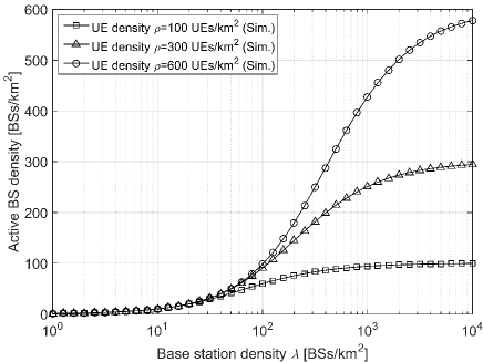
Fig. 2: The active BS density $\tilde{\lambda}$ with various values of $\rho$ for 3GPP Case 1.

Considering Proposition 5, we conduct a bisection search to numerically find the optimal $q^{*}$ for the approximate $\tilde{\lambda}$. Based on the MMSE criterion proposed in Subsection IV-F, we obtain $q^{*}=4.73$, $q^{*}=4.18$ and $q^{*}=3.97$ for the cases of $\rho=100\thinspace\textrm{UEs/km}^{2}$, $\rho=300\thinspace\textrm{UEs/km}^{2}$ and $\rho=600\thinspace\textrm{UEs/km}^{2}$, respectively. In Figs. 3, 4 and 5, we show the average errors on the estimated values of $\tilde{\lambda}$ based on $\tilde{\lambda}^{{\rm{UB}}}$, $\tilde{\lambda}^{{\rm{LB}}}$, and $\lambda_{0}\left(q^{*}\right)$. Note that in these figures, all results are compared against the simulation results shown in Fig. 2, which form the baseline results with zero errors. Also note that as discussed in Subsection IV-B, the exact expression of $\tilde{\lambda}^{{\rm{LB}}}$ is still unknown up to now, but it can be well approximated by $\lambda_{0}\left(3.5\right)$, presented in (20). Hence, the results of $\lambda_{0}\left(3.5\right)$ are displayed in Fig. 4 to represent an lower bound of $\tilde{\lambda}$.

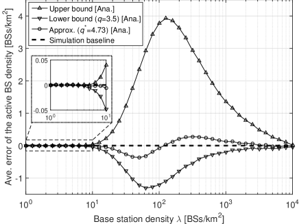
Fig. 3: The average error of the active BS density for 3GPP Case 1 ($\rho=100\,\textrm{UEs/km}^{2}$).

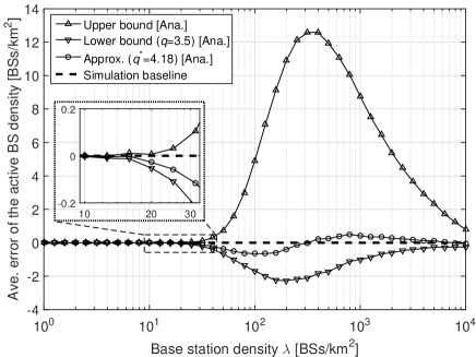
Fig. 4: Average error of the active BS density for 3GPP Case 1 ($\rho=300\,\textrm{UEs/km}^{2}$).

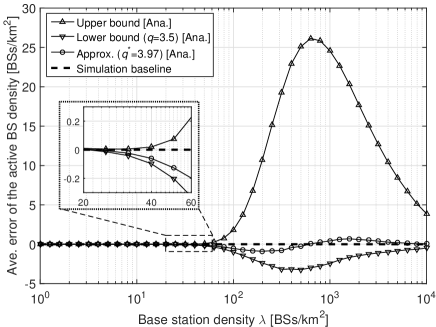
Fig. 5: Average error of the active BS density for 3GPP Case 1 ($\rho=600\,\textrm{UEs/km}^{2}$).

As an example, from Fig. 4 for $\rho=300\thinspace\textrm{UEs/km}^{2}$, we can draw the following conclusions:

• The proposed upper bound $\tilde{\lambda}^{{\rm{UB}}}$ and lower bound $\tilde{\lambda}^{{\rm{LB}}}$ are valid according to the simulation results. More specifically, $\tilde{\lambda}^{{\rm{UB}}}$ and $\tilde{\lambda}^{{\rm{LB}}}$ are always larger (showing positive errors) and smaller (showing negative errors) than the simulation baseline results, respectively.

• $\tilde{\lambda}^{{\rm{UB}}}$ is tighter than $\tilde{\lambda}^{{\rm{LB}}}$ when $\lambda$ is relatively small, e.g., when $\lambda<30\,\textrm{BSs/km}^{2}$.

• $\tilde{\lambda}^{{\rm{LB}}}$ is much tighter than $\tilde{\lambda}^{{\rm{UB}}}$ for dense and ultra-dense SCNs, e.g., $\lambda>100\,\textrm{BSs/km}^{2}$.

• The maximum error associated with $\lambda_{0}\left(q^{*}\right)$ is smaller than those of $\tilde{\lambda}^{{\rm{UB}}}$ and $\tilde{\lambda}^{{\rm{LB}}}$, e.g., when $\rho=300\thinspace\textrm{UEs/km}^{2}$ and $q^{*}=4.18$, the maximum error resulting from $\lambda_{0}\left(q^{*}\right)$ is around $\pm$0.5 $\textrm{BSs/km}^{2}$, while those given by $\tilde{\lambda}^{{\rm{UB}}}$ and $\tilde{\lambda}^{{\rm{LB}}}$ are around 12 $\textrm{BSs/km}^{2}$ and -2 $\textrm{BSs/km}^{2}$, respectively. Hence, $\lambda_{0}\left(q^{*}\right)$ gives a better estimation on $\tilde{\lambda}$ than both $\tilde{\lambda}^{{\rm{UB}}}$ and $\tilde{\lambda}^{{\rm{LB}}}$.

V-B Validation of Theorem 1 for 3GPP Case 1

In Fig. 6, we show the results of $p^{\textrm{cov}}\left(\lambda,\gamma\right)$ when $\rho=300\,\textrm{UEs/km}^{2}$ and $\gamma=0\,\textrm{dB}$, with $q^{*}=4.18$ plugged into Proposition 5. As discussed in Section III, $\rho=300\,\textrm{UEs/km}^{2}$ is a typical density of active UEs in 5G [3], which will be used to evaluate network performance in the following subsections. Note that in our numerical results here and in the following subsections, the proposed analysis is given by Theorem 1 and Proposition 5 with $q^{*}=4.18$. As a benchmark, we also display the results for $\rho=+\infty\,\textrm{UEs/km}^{2}$ with all BSs being active.

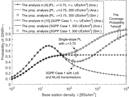
Fig. 6: The coverage probability $p^{\textrm{cov}}\left(\lambda,\gamma\right)$ vs. $\lambda$ for 3GPP Case 1 ($\gamma=0\,\textrm{dB}$, $\rho=300\,\textrm{UEs/km}^{2}$ and $q^{*}=4.18$).

As one can observe, our analytical results well match the simulation results, which validates the accuracy of our analysis. In fact, Fig. 6 is essentially the same as Fig. 1, except that the results for the single-slope path loss model with $\rho=300\,\textrm{UEs/km}^{2}$ are also plotted here for a complete view of the performance behavior. Moreover, Fig. 6 confirms the key observations presented in Section I:

• For the single-slope path loss model with $\rho=+\infty\,\textrm{UEs/km}^{2}$, the coverage probability approaches a constant for dense SCNs, as reported in [4]. As $\rho$ approaches infinity, all BSs are active. Thus, this scenario corresponds to a network condition that does not require the IMC, i.e., the fully loaded network.

• For 3GPP Case 1 with $\rho=+\infty\,\textrm{UEs/km}^{2}$, and when the network is dense enough, i.e., $\lambda>20\,\textrm{BSs/km}^{2}$, the coverage probability decreases as $\lambda$ increases due to the NLoS to LoS transition of interference paths [10], leading to a faster increase of the interference power compared with the signal power.

• For both path loss models with $\rho=300\,\textrm{UEs/km}^{2}$, the coverage probability performance continuously increases toward one, i.e., the Coverage Probability Takeoff. This shows the benefits of the IMC in dense SCNs, as discussed in Sections I and IV.

V-C The ASE Performance for 3GPP Case 1

In Fig. 7, we plot the results of $A^{\textrm{ASE}}\left(\lambda,\gamma_{0}\right)$ when $\rho=300\,\textrm{UEs/km}^{2}$ and $\gamma_{0}=0\,\textrm{dB}$, with $q^{*}=4.18$ plugged into Proposition 5.

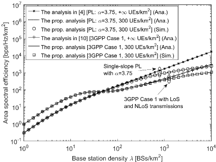
Fig. 7: The ASE $A^{\textrm{ASE}}\left(\lambda,\gamma_{0}\right)$ vs. $\lambda$ for 3GPP Case 1 ($\gamma_{0}=0\,\textrm{dB}$, $\rho=300\,\textrm{UEs/km}^{2}$ and $q^{*}=4.18$).

From Fig. 7, we can draw the following conclusions:

• For 3GPP Case 1, the ASE suffers from a slow growth or even a slight decrease when $\lambda\in\left[20,200\right]\,\textrm{BSs/km}^{2}$ because of the interference transition from NLoS to LoS [10]. Such performance degradation has also been confirmed in Fig. 6.

• After such BS density region of interference transition, for both path loss models with $\rho=300\,\textrm{UEs/km}^{2}$ and the BS IMC, the ASEs monotonically grow as $\lambda$ increases in dense SCNs, but with noticeable performance gaps compared with those with $\rho=+\infty\,\textrm{UEs/km}^{2}$.

• As discussed in Section IV, the takeaway message should not be that the IMC generates an inferior ASE in dense SCNs. Instead, since there is a finite number of the active UEs in the network, some BSs are put to sleep and thus the spatial spectrum reuse in practice is fundamentally limited by $\rho$. The key advantage of the BS IMC is that the per-UE performance should increase with the network densification as exhibited in Fig. 6.

V-D The Performance of 3GPP Case 2

In this subsection, we investigate the performance for 3GPP Case 2 with an alternative path loss model, Rician fading and correlated shadow fading, which have been discussed in Subsection IV-G. Due to the complex modeling of 3GPP Case 2, it is difficult to obtain the analytical results for 3GPP Case 2. Hence, we conduct simulation to investigate 3GPP Case 2 and the results are plotted in Fig. 8. As one can observe from Fig. 8, all the conclusions in Subsections V-B and V-C are qualitatively valid for Fig. 8. Only some quantitative deviations exists, which shows the usefulness of our theoretical analysis to predict the performance trend for dense SCNs with the BS IMC.

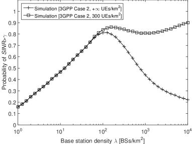
(a) The coverage probability $p^{\textrm{cov}}\left(\lambda,\gamma\right)$ vs. $\lambda$.

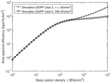
(b) The ASE $A^{\textrm{ASE}}\left(\lambda,\gamma_{0}\right)$ vs. $\lambda$.

Figure 8: Performance for 3GPP Case 2 ($\gamma=0\,\textrm{dB}$ and $\rho=300\,\textrm{UEs/km}^{2}$).

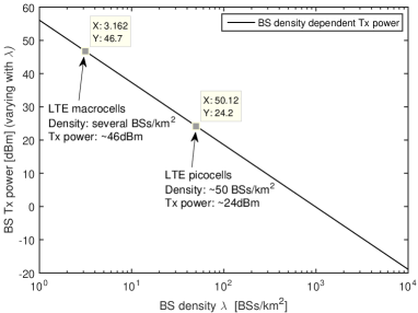
(a) The BS density dependent transmission power in dBm.

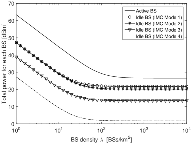
(b) The BS density dependent total power in dBm.

Figure 9: The BS density dependent power configuration.

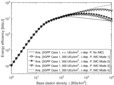
(a) The EE $EE\left(\lambda,\gamma_{0}\right)$ vs. $\lambda$ for 3GPP Case 1.

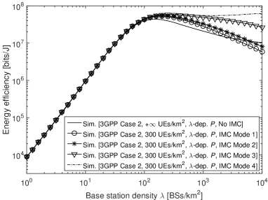
(b) The EE $EE\left(\lambda,\gamma_{0}\right)$ vs. $\lambda$ for 3GPP Case 2.

Figure 10: The EE performance with the BS density dependent power configuration and various IMC modes.

V-E The EE Performance

As discussed in Subsection IV-C, since we consider the realistic EE performance, we should acknowledge the fact that modern telecommunication systems usually work in the interference limited regime and the BS transmission power $P$ should vary with $\lambda$. In this section, we formulate $P$ using the practical power model presented in [3]. Specifically, the transmit power of each BS is configured such that it provides a signal-to-noise-ratio (SNR) of $\eta_{0}=15$ dB at the edge of the average coverage area for a UE with NLoS transmissions, which corresponds to the worst-case path loss. In addition, the distance from a cell-edge UE to its serving BS with an average coverage area is calculated by $r_{0}=\sqrt{\frac{1}{\lambda\pi}}$, which is the radius of an equivalent disk-shaped coverage area with an area size of $\frac{1}{\lambda}$. Therefore, the worst-case pathloss is given by $A^{{\rm{NL}}}r_{0}^{-\alpha^{{\rm{NL}}}}$ and the required transmission power to enable a $\eta_{0}$ dB SNR for this case can be computed as [3]

$$P\left(\lambda\right) = \frac{10^{\frac{\eta_{0}}{10}}P_{{\rm{N}}}}{A^{{\rm{NL}}}r_{0}^{-\alpha^{{\rm{NL}}}}}.$$ (30)

In Fig. 9(a), we plot the BS density dependent transmission power in dBm to illustrate this realistic power configuration when $\eta_{0}=15$ dB. Note that our modeling of $P$ is very practical, covering the cases of macrocells and picocells recommended in the 3GPP Long-Term Evolution (LTE) networks. More specifically, the typical BS densities of LTE macrocells and picocells are respectively several $\textrm{BSs/km}^{2}$ and around 50 $\textrm{BSs/km}^{2}$ [21]. As a result, the typical $P$ of macrocell BSs and picocells BSs are respectively assumed to be 46 dBm and 24 dBm in the 3GPP standards [21], which match well with our modeling of $P$ in Fig. 9(a).

As a result of (30), $P_{{\rm{IMC}}}^{{\rm{TOT}}}\left(\lambda\right)$ and $P_{{\rm{ACT}}}^{{\rm{TOT}}}\left(\lambda\right)$ in (19) are calculated numerically using the Green-Touch power model [15], and the results are displayed in Fig. 9(b) assuming a future SCN BS model in year 2020 and a 10 MHz bandwidth. From this figures, we can draw the following observations:

• The total power of each active BS, i.e., $P_{{\rm{ACT}}}^{{\rm{TOT}}}\left(\lambda\right)$, is always larger than that of each idle BS, i.e., $P_{{\rm{IMC}}}^{{\rm{TOT}}}\left(\lambda\right)$, because some BS component(s) will be deactivated to save energy consumption when a BS enters an idle mode.

• As mentioned in Subsection IV-C, we consider the Green-Touch slow idle mode and the Green-Touch shut-down mode to characterize $P_{{\rm{IMC}}}^{{\rm{TOT}}}\left(\lambda\right)$, which are represented by IMC Mode 1 and IMC Mode 2, respectively. In comparison, IMC Mode 2 consumes less energy than IMC Mode 1 as shown in Fig. 9(b).

• Following [3], we also consider two futuristic idle modes to further characterize $P_{{\rm{IMC}}}^{{\rm{TOT}}}\left(\lambda\right)$, where their energy consumption is 15% (IMC Mode 3) or 1% (IMC Mode 4) of that of the Green-Touch slow idle mode (IMC Mode 1). The former mode (IMC Mode 3) accounts less energy consumption than the Green-Touch shut-down mode (IMC Mode 2), and the latter mode (IMC Mode 4) assumes that a BS consumes almost nothing.

Based on the results of $P_{{\rm{IMC}}}^{{\rm{TOT}}}\left(\lambda\right)$ and $P_{{\rm{ACT}}}^{{\rm{TOT}}}\left(\lambda\right)$ displayed in Fig. 9(b), in Fig. 10 we plot the EE performance for 3GPP Case 1 and Case 2 when $\rho=+\infty\,\textrm{UEs/km}^{2}$ without the IMC and $\rho=300\,\textrm{UEs/km}^{2}$ with various IMC modes.

Here, Fig. 10(a) shows our analytical results for 3GPP Case 1 based on the ASE performance exhibited in Subsection V-C, while Fig. 10(b) displays our simulation results for 3GPP Case 2 based on the ASE performance discussed in Subsection V-D. Although 3GPP Case 2 is more realistic than 3GPP Case 1, as one can observe from Fig. 10(a) and Fig. 10(b), the EE performance shows the same trend in both figures, only with some quantitative deviations. Again, this indicates the usefulness of our theoretical analysis to predict the network performance trend for dense SCNs with the BS IMC.

As discussed in Subsection IV-C, $\tilde{\lambda}$ represents the active BS density, which is a function of $\lambda$ due to the BS IMC. Hence, $\lambda$ is used as the x-axis instead of $\tilde{\lambda}$ in Fig. 10.

From Fig. 10, we can draw the following conclusions:

• As predicted in Subsection V-C, the baseline scheme with $\rho=+\infty\,\textrm{UEs/km}^{2}$, where all BSs are active, is the least energy efficient scheme for most BS densities, because each BS suffers from a diminishing EE return with the network densification due to the deteriorating performance of the coverage probability as the BS density increases (see Fig. 6). Such deteriorating performance is caused by the interference path transition from NLoS to LoS as discussed in previous sections.

• On the other hand, the EE performance of various IMC modes benefits from the Coverage Probability Takeoff, which improves the performance of each active BS as the SCN densifies, and thus the IMC scheme outperforms the baseline scheme in terms of the EE. When comparing the EE performance of different IMC modes, it can be seen that the lower the power consumption in the idle mode exhibited in Fig. 9(b), the larger the EE of such IMC mode.

• When using the Green-Touch slow idle mode (IMC Mode 1) and the Green-Touch shut-down mode (IMC Mode 2), the EE first increases and then decreases with the network densification. This decrease is because the increase in the ASE provided by the Coverage Probability Takeoff is not large enough to compensate the increase in power consumption that the dense network brings about, mostly because idle BSs following the Green-Touch power models still consume a non-negligible amount of energy. Nevertheless, the schemes with the IMC are superior to the baseline scheme. In more detail, when $\lambda=10^{3}\,\textrm{BSs/km}^{2}$, the Green-Touch slow idle mode (IMC Mode 1) and the Green-Touch shut-down mode (IMC Mode 2) can achieve EE performance of $17.2\,\textrm{Mbits/J}$ and $20.2\,\textrm{Mbits/J}$, respectively, which are around two times the EE of the baseline scheme, i.e., $9.95\,\textrm{Mbits/J}$.

• When considering the EE of the futuristic IMC Mode 3 and IMC Mode 4, the above trend starts changing. For IMC Mode 3, the EE is always larger than that of the baseline scheme across all BS densities, as BSs consume much less energy in this idle mode. For IMC Mode 4, idle BSs barely consume any energy, and thus the above trend fundamentally alters, i.e., as the network evolves into an ultra-dense one, the EE continuously increases. As a result, when $\lambda=10^{3}\,\textrm{BSs/km}^{2}$, IMC Mode 3 and IMC Mode 4 can achieve EE performance of $29.6\,\textrm{Mbits/J}$ and $33.6\,\textrm{Mbits/J}$, respectively, which triple that of the baseline scheme, i.e., $9.95\,\textrm{Mbits/J}$. This help us to conclude that idle mode schemes similar to IMC Mode 4 are needed to ensure an energy-efficient deployment of dense SCNs in 5G and beyond.

V-F Future Work of Ultra-Dense SCNs

In this subsection, we indicate several research directions for ultra-dense SCNs:

• It would be good to study a proportional fair (PF) scheduler in ultra-dense networks [22]. Currently, in stochastic geometry analyses, usually a typical UE is randomly chosen for the performance analysis, which implies that a round Robin (RR) scheduler is employed in each BS. However, in the 3GPP performance evaluations, the typical UE is not chosen randomly and a PF scheduler is often used as an appealing scheduling technique to smartly serve UEs that can offer a better system throughput than the RR scheduler.

• It would be good to study the near-field effect in the context of ultra-dense networks. In particular, the Rayleigh distance as investigated in [23], should be considered in the extremely ultra-dense networks because the BS-to-UE distance becomes very small as the network densifies.

• A very recent discovery shows the 5G network capacity might decrease to zero if the antenna height difference between BSs and UEs is non-zero [24]. Hence, it is of great interest to study whether the BS IMC can help to mitigate such network capacity crash.

• It would be good to study a non-uniform distribution of BSs with some constraints on the minimum BS-to-BS distance [25]. In stochastic geometry analyses, BSs are usually assumed to be uniformly deployed in the interested network area. However, in the 3GPP performance evaluations, small cell clusters are often considered, and it is forbidden to place any two BSs too close to each other. Such assumption is in line with the realistic network planning to avoid strong inter-cell interference.

• It would be good to study ultra-dense networks in new emerging network scenarios, such as heterogeneous networks [26], distributed networks [27], high mobility applications [28, 29], device to device (D2D) communications [30, 31, 32], body area networks [33], unmanned aerial vehicles [34], etc.

VI Conclusion

In this paper, we have studied the performance impact of the IMC on dense SCNs considering probabilistic LoS and NLoS transmissions. The impact is significant on the coverage probability performance, i.e., as the BS density surpasses the UE density, the coverage probability continuously increases toward one in dense SCNs (the Coverage Probability Takeoff), addressing the critical issue of coverage probability decrease that may lead to “the death of 5G”.

Two important conclusions have been drawn from our study: (i) the active BS density with the mentioned probabilistic LoS and NLoS path loss model is lower-bounded by that with a simplistic single-slope path loss model derived in [5], and (ii) such lower bound, shown in [5], is tight, especially for dense SCNs. This shows a simple way of studying the IMC in dense SCNs.

Moreover, from our studies based on practical power models of the Green-Touch project and realistic 3GPP propagation models, we conclude that idle mode schemes similar to IMC Mode 4 are needed to ensure an energy-efficient deployment of dense SCNs in 5G and beyond.

Appendix A: Proof of Lemma 2

To prove Lemma 2, first we would like to emphasize the insights or the proof sketch of Theorem 1 as follows. In (8), $T_{n}^{{\rm{L}}}$ and $T_{n}^{{\rm{NL}}}$ are the components of the coverage probability for the case when the signal comes from the $n$-th piece LoS path and for the case when the signal comes from the $n$-th piece NLoS path, respectively. The calculation of $T_{n}^{{\rm{L}}}$ is based on (9) and (13), which are explained in the sequel.

• In (9), $f_{R,n}^{{\rm{L}}}\left(r\right)$ characterizes the geometrical density function of the typical UE with no other LoS BS and no NLoS BS providing a better link to the typical UE than its serving BS (a BS with the $n$-th piece LoS path).

• In (13), $\exp\left(-\frac{\gamma P_{{\rm{N}}}}{P\zeta_{n}^{{\rm{L}}}\left(r\right)}\right)$ is the probability that the signal power exceeds the noise power by a factor of at least $\gamma$, and $\mathscr{L}_{I_{{\rm{agg}}}}^{{\rm{L}}}\left(\frac{\gamma}{P\zeta_{n}^{{\rm{L}}}\left(r\right)}\right)$ (further computed by (14)) is the probability that the signal power exceeds the aggregate interference power by a factor of at least $\gamma$.

• Since $h$ follows an exponential distribution, the product of the above probabilities yields the probability that the signal power exceeds the sum power of the noise and the aggregate interference by a factor of at least $\gamma$.

The calculation of $T_{n}^{{\rm{NL}}}$ is based on (10) and (15). The interpretation of (10) and (15) are similar to that for the calculation of $T_{n}^{{\rm{L}}}$.

Hence, Lemma 2 is valid because:

• For $p^{\textrm{cov}}\left(\lambda,\gamma\right)$ with the BS IMC and that with all BSs being active, (9) and (10) are the same, indicating an increasing signal power as $\lambda$ grows. This is because that as $\lambda$ increases, to achieve the same $f_{R,n}^{{\rm{L}}}\left(r\right)$ in (9) or $f_{R,n}^{{\rm{NL}}}\left(r\right)$ in (10), $r$ has to be reduced, meaning that the typical UE will connect to a nearer BS with a larger signal power.

• For $p^{\textrm{cov}}\left(\lambda,\gamma\right)$ with the BS IMC, $\tilde{\lambda}$ is plugged into (14) and (16), while for $p^{\textrm{cov}}\left(\lambda,\gamma\right)$ with all BSs being active, $\lambda$ was used in (14) and (16) [10]. The former case is able to generate a larger $p^{\textrm{cov}}\left(\lambda,\gamma\right)$ than the latter one, since $\tilde{\lambda}\leq\lambda$ and $\exp\left(-x\right)$ is a decreasing function with respect to $x$ in (14) and (16). The intuition is that the aggregate interference power of the former case with the BS IMC is less than that of the latter case without, since $\mathscr{L}_{I_{{\rm{agg}}}}^{{\rm{L}}}\left(\frac{\gamma}{P\zeta_{n}^{{\rm{L}}}\left(r\right)}\right)$ in (14) and $\mathscr{L}_{I_{{\rm{agg}}}}^{{\rm{NL}}}\left(\frac{\gamma}{P\zeta_{n}^{{\rm{NL}}}\left(r\right)}\right)$ in (16) capture the impact of the aggregate interference on $p^{\textrm{cov}}\left(\lambda,\gamma\right)$, as discussed above.

Appendix B: Proof of Theorem 3

For clarity, the main idea of our proof is summarized as follows:

• We will prove that from a typical UE’s point of view, the equivalent BS density of the considered UAS based on probabilistic LoS and NLoS transmissions is larger than that of the nearest-distance UAS based on single-slope path loss transmissions.

• Considering such increased equivalent BS density and the fact that a larger $\lambda$ always leads to a larger $\tilde{\lambda}$ due to a higher BS diversity, we can conclude that $\tilde{\lambda}\geq\tilde{\lambda}^{{\rm{minDis}}}$.

First, let us consider a baseline scenario that all BSs only have NLoS links to UEs. In such scenario, the nearest-distance UAS is a reasonable one and the active BS density should be characterized by $\tilde{\lambda}^{{\rm{minDis}}}$ [5].

Next, for the proposed scenario with probabilistic LoS and NLoS transmissions, we consider a typical UE $k$ and an arbitrary BS $b$ located at a distance $r$ from UE $k$. Due to probabilistic LoS and NLoS transmissions, such BS $b$ can be virtually split into two probabilistic BSs, i.e., a LoS BS $b^{{\rm{L}}}$ to UE $k$ with a probability of $\textrm{Pr}^{\textrm{L}}\left(r\right)$ and a NLoS BS $b^{{\rm{NL}}}$ to UE $k$ with a probability of $\left(1-\textrm{Pr}^{\textrm{L}}\left(r\right)\right)$. Compared with the baseline scenario that all BSs only have NLoS links to UEs, the equivalent distance from the NLoS BS $b^{{\rm{NL}}}$ to UE $k$ remains to be $r$, while that from the LoS BS $b^{{\rm{L}}}$ to UE $k$ can be calculated as $r_{1}=\underset{r_{1}}{\arg}\left\{\zeta^{{\rm{NL}}}\left(r_{1}\right)=\zeta^{{\rm{L}}}\left(r\right)\right\}$, which is shown in (11). The calculation of $r_{1}$ is straightforward because it finds an equivalent position for the LoS BS $b^{{\rm{L}}}$ as if the LoS transmission is replaced with a NLoS one. Since a LoS transmission is always stronger than a NLoS one, we have $r_{1}<r$.

Consequently, in a disk area centered on UE $k$ with a radius of $r_{1}$, the equivalent BS number is increased by at least $\textrm{Pr}^{\textrm{L}}\left(r\right)$, which is a non-negative value. Due to the arbitrary value of $r_{1}$, from a typical UE’s point of view, the equivalent BS density of the considered UAS based on probabilistic LoS and NLoS transmissions is larger than that of the nearest-distance UAS based on single-slope path loss transmissions. In other words, the existence of LoS BSs provides more candidate BSs for a typical UE to connect with, and thus the equivalent BS density increases for each UE.

Finally, we can conclude that $\tilde{\lambda}\geq\tilde{\lambda}^{{\rm{minDis}}}\approx\lambda_{0}\left(q\right)$, because a larger $\lambda$ leads to a larger $\tilde{\lambda}$ due to a higher BS diversity.

Appendix C: Proof of Theorem 4

For clarity, the main idea of our proof is summarized as follows:

• First, we derive an conditional probability that an arbitrary UE $w$ is not associated with an arbitrary BS $b$ conditioned on the distance between UE $w$ and BS $b$ being $r$. Such conditional probability is denoted by ${\rm{Pr}}\left[\left.w\nsim b\right|r\right]$.

• Next, we derive an unconditional probability that an arbitrary UE $w$ is not associated with an arbitrary BS $b$ by performing an integral over $r$ considering the uniform distribution of UEs in the considered network. Such unconditional probability is denoted by ${\rm{Pr}}\left[w\nsim b\right]$.

• Finally, we derive a lower bound of the probability that every UE is not associated with an arbitrary BS $b$, so that BS $b$ should switch off its transmission. The lower bound of the BS deactivation probability is then translated to an upper bound of the active BS density, i.e., $\tilde{\lambda}$.

For convenience, the PDF of the distance between a typical UE and its serving BS, i.e., $\left\{f_{R,n}^{\textrm{L}}\left(r\right)\right\}$ and $\left\{f_{R,n}^{\textrm{NL}}\left(r\right)\right\}$ are stacked into piece-wise functions written as

$$f_{R}^{Path}\left(r\right)=\begin{cases}f_{R,1}^{Path}\left(r\right),&\textrm{when }0\leq r\leq d_{1}\\ f_{R,2}^{Path}\left(r\right),&\textrm{when }d_{1}<r\leq d_{2}\\ \vdots&\vdots\\ f_{R,N}^{Path}\left(r\right),&\textrm{when }r>d_{N-1}\end{cases},$$ (31)

where the string variable $Path$ takes the value of “L” and “NL” for the LoS and the NLoS cases, respectively.

Based on $f_{R}^{Path}\left(r\right)$, we define the cumulative distribution function (CDF) of $r$ as

$$F_{R}^{Path}\left(r\right)=\int_{0}^{r}f_{R}^{Path}\left(v\right)dv.$$ (32)

In addition, we define the sum of $F_{R}^{{\rm{L}}}\left(r\right)$ and $F_{R}^{{\rm{NL}}}\left(r\right)$ as $F_{R}\left(r\right)=F_{R}^{{\rm{L}}}\left(r\right)+F_{R}^{{\rm{NL}}}\left(r\right)$, which is the CDF of the UE association distance of the presented UAS. Obviously, we have $F_{R}\left(+\infty\right)=1$. Then, ${\rm{Pr}}\left[\left.w\nsim b\right|r\right]$ can be calculated by (25) because ${\rm{Pr}}\left[\left.w\nsim b\right|r\right]$ should be the sum of the probabilities of the following two events that lead to the event $\left[\left.w\nsim b\right|r\right]$:

• The first term of (25): The link between UE $w$ and BS $b$ is a LoS one with a probability of ${\rm{Pr}}^{{\rm{L}}}\left(r\right)$ while UE $w$ is associated with another LoS/NLoS BS that is stronger than BS $b$ with a probability of $\left[F_{R}^{{\rm{L}}}\left(r\right)+F_{R}^{{\rm{NL}}}\left(r_{1}\right)\right]$, with $F_{R}^{{\rm{L}}}\left(r\right)$ and $F_{R}^{{\rm{NL}}}\left(r_{1}\right)$ corresponding to the cases of a stronger LoS BS and a stronger NLoS BS, respectively;

• The second term of (25): The link between UE $w$ and BS $b$ is a NLoS one with a probability of $\left[1-{\rm{Pr}}^{{\rm{L}}}\left(r\right)\right]$ while UE $w$ is associated with another LoS/NLoS BS that is stronger than BS $b$ with a probability of $\left[F_{R}^{{\rm{L}}}\left(r_{2}\right)+F_{R}^{{\rm{NL}}}\left(r\right)\right]$, with $F_{R}^{{\rm{L}}}\left(r_{2}\right)$ and $F_{R}^{{\rm{NL}}}\left(r\right)$ corresponding to the cases of a stronger LoS BS and a stronger NLoS BS, respectively.

Next, for an arbitrary BS $b$, we suppose that all its candidate UEs are randomly distributed in a disk $\Omega$ centered on BS $b$ with a radius of $r_{\textrm{max}}>0$. Then, for an arbitrary UE $w$ inside the disk $\Omega$, ${\rm{Pr}}\left[w\nsim b\right]$ can be computed by (24), where $\frac{2r}{r_{\textrm{max}}^{2}}$ is the distribution density function with respect to $r$ for UE $w$ [4], because UEs are assumed to be uniformly distributed.

Finally, the number of candidate UEs inside disk $\Omega$, denoted by $K$, should follow a Poisson distribution with a parameter of $\lambda_{\Omega}=\rho\pi r_{\textrm{max}}^{2}$. Thus, the probability mass function (PMF) of $K$ can be written as [35]

$$f_{K}\left(k\right)=\frac{\lambda_{\Omega}^{k}e^{-\lambda_{\Omega}}}{k!},\quad k\in\left\{0,1,2,\dots,\right\}.$$ (33)

Hence, the probability that BS $b$ should be muted, i.e., no UE is associated with BS $b$, can be computed by (23).

It is very important to note that (23) ignores the correlation between nearby UEs inside disk $\Omega$, i.e., a UE $k$ not associated with BS $b$ may imply that a nearby UE $k^{\prime}$ should have a large probability of also not connecting with BS $b$, due to the possible existence of a high-link-quality BS near UEs $k$ and $k^{\prime}$. Therefore, $Q^{{\rm{off}}}$ under-estimates the probability that BS $b$ should be muted, and thus the active BS density $\tilde{\lambda}$ can be upper-bounded by $\lambda\left(1-Q^{{\rm{off}}}\right)$, which concludes our proof.

References

- [1] CISCO, “Cisco visual networking index: Global mobile data traffic forecast update (2015-2020),” Feb. 2016.
- [2] 3GPP, “TR 36.872: Small cell enhancements for E-UTRA and E-UTRAN - Physical layer aspects,” Dec. 2013.
- [3] D. L pez-P rez, M. Ding, H. Claussen, and A. Jafari, “Towards 1 Gbps/UE in cellular systems: Understanding ultra-dense small cell deployments,” IEEE Communications Surveys Tutorials, vol. 17, no. 4, pp. 2078–2101, Jun. 2015.
- [4] J. Andrews, F. Baccelli, and R. Ganti, “A tractable approach to coverage and rate in cellular networks,” IEEE Transactions on Communications, vol. 59, no. 11, pp. 3122–3134, Nov. 2011.
- [5] S. Lee and K. Huang, “Coverage and economy of cellular networks with many base stations,” IEEE Communications Letters, vol. 16, no. 7, pp. 1038–1040, Jul. 2012.
- [6] 3GPP, “TR 36.828: Further enhancements to LTE Time Division Duplex for Downlink-Uplink interference management and traffic adaptation,” Jun. 2012.
- [7] Spatial Channel Model AHG, “Subsection 3.5.3, Spatial Channel Model Text Description V6.0,” Apr. 2003.
- [8] X. Zhang and J. Andrews, “Downlink cellular network analysis with multi-slope path loss models,” IEEE Transactions on Communications, vol. 63, no. 5, pp. 1881–1894, May 2015.
- [9] T. Bai and R. Heath, “Coverage and rate analysis for millimeter-wave cellular networks,” IEEE Transactions on Wireless Communications, vol. 14, no. 2, pp. 1100–1114, Feb. 2015.
- [10] M. Ding, P. Wang, D. L pez-P rez, G. Mao, and Z. Lin, “Performance impact of LoS and NLoS transmissions in dense cellular networks,” IEEE Transactions on Wireless Communications, vol. 15, no. 3, pp. 2365–2380, Mar. 2016.
- [11] J. Andrews and A. Gatherer, “Will densification be the death of 5G?” IEEE ComSoc Technology News, May 2015.
- [12] Z. Luo, M. Ding, and H. Luo, “Dynamic small cell on/off scheduling using stackelberg game,” IEEE Communications Letters, vol. 18, no. 9, pp. 1615–1618, Sept 2014.
- [13] C. Li, J. Zhang, and K. Letaief, “Throughput and energy efficiency analysis of small cell networks with multi-antenna base stations,” IEEE Transactions on Wireless Communications, vol. 13, no. 5, pp. 2505–2517, May 2014.
- [14] T. Zhang, J. Zhao, L. An, and D. Liu, “Energy efficiency of base station deployment in ultra dense hetnets: A stochastic geometry analysis,” IEEE Wireless Communications Letters, vol. 5, no. 2, pp. 184–187, Apr. 2016.
- [15] C. Desset, B. Debaillie, and F. Louagie, “Flexible Power Model of Future Base Stations: System Architecture Breakdown and Parameters,” Green Touch.
- [16] M. Ding, D. L pez-P rez, G. Mao, and Z. Lin, “Study on the idle mode capability with LoS and NLoS transmissions,” IEEE Globecom 2016, pp. 1–6, Dec. 2016.
- [17] H. S. Dhillon, R. K. Ganti, F. Baccelli, and J. G. Andrews, “Modeling and analysis of K-tier downlink heterogeneous cellular networks,” IEEE Journal on Selected Areas in Communications, vol. 30, no. 3, pp. 550–560, Apr. 2012.
- [18] M. D. Renzo, W. Lu, and P. Guan, “The intensity matching approach: A tractable stochastic geometry approximation to system-level analysis of cellular networks,” IEEE Transactions on Wireless Communications, vol. 15, no. 9, pp. 5963–5983, Sep. 2016.
- [19] M. Ding, D. L pez-P rez, G. Mao, P. Wang, and Z. Lin, “Will the area spectral efficiency monotonically grow as small cells go dense?” IEEE GLOBECOM 2015, pp. 1–7, Dec. 2015.
- [20] R. L. Burden and J. D. Faires, Numerical Analysis (3rd Ed.). PWS Publishers, 1985.
- [21] 3GPP, “TR 36.814: Further advancements for E-UTRA physical layer aspects,” Mar. 2010.
- [22] A. H. Jafari, D. L pez-P rez, M. Ding, and J. Zhang, “Study on scheduling techniques for ultra dense small cell networks,” Vehicular Technology Conference (VTC Fall), 2015 IEEE 82nd, pp. 1–6, Sep. 2015.
- [23] S. Wu, C. X. Wang, e. H. M. Aggoune, M. M. Alwakeel, and Y. He, “A non-stationary 3-D wideband twin-cluster model for 5G massive MIMO channels,” IEEE Journal on Selected Areas in Communications, vol. 32, no. 6, pp. 1207–1218, Jun. 2014.
- [24] M. Ding and D. L pez-P rez, “Please Lower Small Cell Antenna Heights in 5G,” IEEE Globecom 2016, pp. 1–6, Dec. 2016.
- [25] M. Ding, D. L pez-P rez, G. Mao, and Z. Lin, “Microscopic analysis of the uplink interference in FDMA small cell networks,” IEEE Trans. on Wireless Communications, vol. 15, no. 6, pp. 4277–4291, Jun. 2016.
- [26] T. Zhang, J. Zhao, L. An, and D. Liu, “Energy efficiency of base station deployment in ultra dense HetNets: A stochastic geometry analysis,” IEEE Wireless Communications Letters, vol. 5, no. 2, pp. 184–187, Apr. 2016.
- [27] X. Ge, S. Tu, G. Mao, C. X. Wang, and T. Han, “5G ultra-dense cellular networks,” IEEE Wireless Communications, vol. 23, no. 1, pp. 72–79, Feb. 2016.
- [28] X. Ge, J. Ye, Y. Yang, and Q. Li, “User mobility evaluation for 5G small cell networks based on individual mobility model,” IEEE Journal on Selected Areas in Communications, vol. 34, no. 3, pp. 528–541, Mar. 2016.
- [29] R. Arshad, H. ElSawy, S. Sorour, T. Y. Al-Naffouri, and M. S. Alouini, “Handover management in dense cellular networks: A stochastic geometry approach,” 2016 IEEE International Conference on Communications (ICC), pp. 1–7, May 2016.
- [30] J. Liu, Y. Kawamoto, H. Nishiyama, N. Kato, and N. Kadowaki, “Device-to-device communications achieve efficient load balancing in LTE-advanced networks,” IEEE Wireless Communications, vol. 21, no. 2, pp. 57–65, Apr. 2014.
- [31] J. Liu, N. Kato, J. Ma, and N. Kadowaki, “Device-to-device communication in LTE-Advanced networks: A survey,” IEEE Communications Surveys Tutorials, vol. 17, no. 4, pp. 1923–1940, Fourth-quarter 2015.
- [32] J. Liu, H. Nishiyama, N. Kato, and J. Guo, “On the outage probability of device-to-device-communication-enabled multichannel cellular networks: An RSS-threshold-based perspective,” IEEE Journal on Selected Areas in Communications, vol. 34, no. 1, pp. 163–175, Jan. 2016.
- [33] W. Sun, Y. Ge, Z. Zhang, and W. C. Wong, “An analysis framework for interuser interference in IEEE 802.15.6 body sensor networks: A stochastic geometry approach,” IEEE Transactions on Vehicular Technology, vol. 65, no. 10, pp. 8567–8577, Oct. 2016.
- [34] A. Fotouhi, M. Ding, and M. Hassan, “Dynamic base station repositioning to improve performance of drone small cells,” 2016 IEEE Globecom Workshops, pp. 1–6, Dec. 2016.
- [35] J. G. Proakis, Digital Communications (4th Ed.). New York: McGraw-Hill, 2000.