The reconstruction of sound speed in the Marmousi model by the boundary control method

Abstract

We present the results on numerical testing of the Boundary Control Method in the sound speed determination for the acoustic equation on semiplane. This method for solving multidimensional inverse problems requires no a priory information about the parameters under reconstruction. The application to the realistic Marmousi model demonstrates that the boundary control method is workable in the case of complicated and irregular field of acoustic rays. By the use of the chosen boundary controls, an ‘averaged’ profile of the sound speed is recovered (the relative error is about $10-15\%$). Such a profile can be further utilized as a starting approximation for high resolution iterative reconstruction methods.

Key words: acoustics, inverse problem, modelling

1 Introduction

The Boundary Control Method (BCM) is ab initio approach to multidimensional inverse problems based on ideas and results of control theory, asymptotic methods (for propagation of discontinuities), functional analysis, and geometry: see (Belishev, 1988, 1997, 2007) and references therein. Its simple and clear mathematical background makes the method of rather general scope. In particular, the BCM is developed for acoustics (Belishev, 1988), electrodynamics (Belishev and Glasman, 2001), Shrödinger equation (Avdonin and Belishev, 2005), 1D Dirac system (Belishev and Mikhailov, 2014), 1D two-velocity system (Belishev and Ivanov, 2005), reconstruction of Riemannian manifolds (Belishev, 1997, Belishev and Demchenko, 2011), metric graphs (Belishev and Vakulenko, 2006), and other dynamic systems.

The BCM provides time optimal step-by-step reconstruction procedure, which requires no ad hoc assumptions about the sound speed profile. It works in the case of data given on a part of the domain boundary. Variants of BCM are developed and numerically tested for different problems in (Belishev et al., 1997, Belishev and Gotlib, 1999, Pestov et al., 2010, 2012, Pestov, 2012, 2014, Oksanen, 2013).

There exist another (not optimal) direct reconstruction methods which are numerically (and experimentally) tested: see (Kabanikhin and Shishlenin, 2004, Kabanikhin et al., 2005, Kabanikhin and Shishlenin, 2011, Belina and Klibanov, 2008, 2012) and references therein. A time optimal and data optimal approach by V. G. Romanov (Romanov, 1996) is not implemented and tested yet.

The goal of this paper is to provide a concise and transparent outline of dynamic variant of BCM for the acoustic equation and discuss recent numerical results on the sound speed reconstruction in several test cases. A rigorous and detailed exposition of the method can be found in the reviews (Belishev, 1997, 2007). Previous results on numerical testing of the same BCM version for the wave equation are published in (Belishev et al., 1997, Belishev and Gotlib, 1999) and (Belishev et al., 2016).

We consider a dynamic system governed by the acoustic equation in a domain $\Omega\subset{\bf R}^{n}$ ($n\geq 2$) with the boundary $\Gamma$:

$$\left[\partial_{t}^{2}-c^{2}\Delta\right]u=0 \rm in\,\,\Omega\times(0,T)$$ (1)

$$u\big{|}_{t=0}=\partial_{t}u\big{|}_{t=0}=0 \rm in\,\,\Omega$$ (2)

$$u\big{|}_{\Sigma^{T}}=f.$$ (3)

Here $t$ is a time, $x=(x^{1},\dots,x^{n})\in{\bf R}^{n}$ are Cartesian coordinates, $c=c(x)>0$ is a speed of sound, $\Sigma^{T}:=\Gamma\times[0,T]$. A solution (wave) $u=u^{f}(x,t)$ describes a perturbation of the acoustic pressure in the medium caused by a boundary source (control) $f$ acting from $\Gamma$ during the probing time $T$. An ‘input $\rightarrow$ output’ correspondence of the system is realized by a response operator $R^{T}:f\mapsto\partial_{\nu}u^{f}|_{\Sigma^{T}}$ ($\nu$ is the outward normal to $\Gamma$).

Let $R^{2T}$ be the response operator of the same system (1)–(3) with the double probing time $2T$. Due to the finiteness of the wave propagation speed, operator $R^{2T}$ is determined by the values of $c$ in the near-boundary subdomain $\Omega^{T}$ filled up with waves at the moment $t=T$, and does not depend on the behavior of $c$ in $\Omega\backslash\Omega^{T}$. Such a local character of the dependence motivates the following relevant statement of the inverse problem: given $R^{2T}$ recover the speed $c$ in the subdomain $\Omega^{T}$.

To solve this problem, the BCM exploits certain subtle properties of the waves. The principal role is played by a completeness of waves, which is interpreted in control theory as a boundary controllability of the system (1)–(3). Also, the geometrical optics is used for extracting information about the medium from the wave field jumps propagating through $\Omega$ and being detected on $\Gamma$. The crucial point is that, for the given controls $f,g$, the integrals of the form $\int_{\Omega}\mathrm{d}x\,c^{-2}u^{f}u^{g}$ are determined by the inverse data, i.e., can be computed via operator $R^{2T}$. These facts enable the external observer to recover the images of waves on the space-time surface $\Sigma^{T}$. Roughly speaking, an image is just a wave written in the ray coordinates, which are associated with the acoustic rays orthogonal to $\Gamma$. Along with the wave images, the observer can recover images of the Cartesian coordinate functions and, thus, determine the connection between the Cartesian and ray coordinates. Such a connection easily determines the sound speed $c$ in $\Omega^{T}$ that solves the inverse problem. In the paper, we propose the procedure, which recovers $c$ in a ray tube $B^{T}_{\sigma}\subset\Omega$ covered by acoustic rays, which emanate from a part $\sigma\subset\Gamma$. In capacity of the inverse data, the response $R^{2T}f$ on the controls $f$ acting on $\sigma$, is used.

The paper is organized as follows. In the first three sections we introduce the reader to main notions and known results, which form a ’language‘ of the boundary control method. In Section 2 we describe a convenient and natural system of semigeodesic coordinates. In Section 3 the notions of control theory are applied to the dynamic system (1)–(3). In Section 4 we use the of geometric optics formulas for propagation of discontinuities to derive the amplitude formula, which is a main computational device of BCM. In Section 5 we combine all findings and provide step-by-step reconstruction procedure for the speed of sound. Finally, in Section 6 some numerical results of application of BCM to several test cases are presented and discussed.

2 Geometry

2.1 Metric

The speed of sound $c$ determines a $c$-metric in $\Omega$ with the distance between points

$$\tau(x,y):=\text{inf}\int\limits_{x}^{y}\,\frac{\mathrm{d}l}{c}\,,$$ (4)

where the infimum is taken over all smooth curves connecting $x$ and $y$, $\mathrm{d}l$ is a length element in ${\bf R}^{n}$. In dynamics, $\tau(x,y)$ coincides with the travel time needed for a wave initiated at $x$ to reach $y$. The geodesics of the $c$-metric are the curves realizing the infimum in (4).

Let $\sigma\subseteq\Gamma$ be an open set at the boundary. In what follows, unless otherwise specified, we assume that $\sigma$ is fixed. The travel time needed for a wave initiated on $\sigma$ to reach a point $x\in\Omega$ is called an eikonal:

$$\tau_{\sigma}(x):=\min_{y\in\sigma}\,\tau(y,x).$$ (5)

Fix a $\xi\geq 0$. The level set of the eikonal

$$\Gamma^{\xi}_{\sigma}:=\left\{x\in\Omega\mid\tau_{\sigma}(x)=\xi\right\}$$ (6)

is a wave front surface that bounds (together with $\Gamma$) a subdomain filled by waves, which move into $\Omega$ from $\sigma$, at $t=\xi$,

$$\Omega^{\xi}_{\sigma}:=\left\{x\in\Omega\mid\tau_{\sigma}(x)<\xi\right\}.$$ (7)

In the case $\sigma=\Gamma$ we simplify the notation and write $\tau,\,\Gamma^{\xi},\,\Omega^{\xi}$.

2.2 Ray coordinates

Fix a point $\gamma\in\sigma$. Let $x(\gamma,\xi)$ be the endpoint of the geodesic curve in $c$-metric (ray) starting from $\gamma$ orthogonally to $\sigma$ and parametrized by its $c$-length $\xi$. For $T>0$, all such rays starting from $\sigma$ cover a subdomain (tube)

$$B^{T}_{\sigma}:=\bigcup_{\gamma\in\sigma}\bigcup_{0\leq\xi\leq T}x(\gamma,\xi).$$

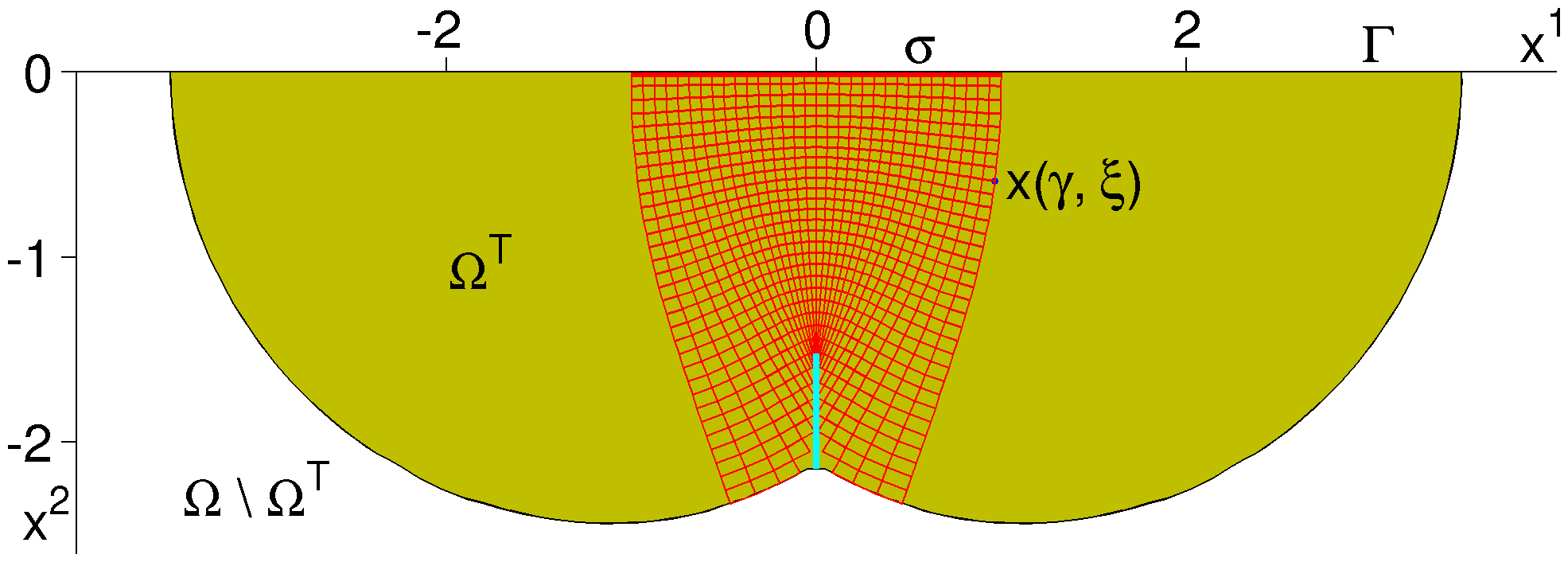
Figure 1: A typical simple geometry of rays on semiplane: domain $\Omega^{T}$ (fill), semigeodesic coordinates $x(\gamma,\xi)$ (mesh), cut locus (vertical line). The speed of sound $c(x)$ is taken from Section 6.1 with $\sigma=\{x\in\Gamma\mid|x^{1}|<1\}$, $T=2.5$.

We say $\sigma$ to be a bottom of the tube. A typical picture of the ray field in the case of the semiplane is shown in Fig. 1, here $\Omega=\{x\mid x^{2}<0\}$, $\Gamma=\{x\mid x^{2}=0\}$, $\sigma=\{x\in\Gamma\mid|x^{1}|<1\}$, and speed of sound $c(x)$ is taken from Section 6.1.

If $T$ is sufficiently small then the ray family is regular: only one ray passes through any point in $B^{T}_{\sigma}$. In this case, to each $x\in B^{T}_{\sigma}$ we preassign the pair $(\gamma,\xi)$ such that $x=x(\gamma,\xi)$. This pair is called the semigeodesic (ray) coordinates of $x$.

The connection between the ray and Cartesian coordinates can be easily calculated by solving the Euler-Lagrange equations for functional (4): if $x=x(\gamma,\xi)=\left(x^{1}(\gamma,\xi),\dots,x^{n}(\gamma,\xi)\right)$ then

$$\frac{\partial x^{k}}{\partial\xi}=c^{2}\,v^{k},\quad\frac{\partial v^{k}}{\partial\xi}=-\frac{1}{c}\,\frac{\partial c}{\partial x^{k}}\,,\qquad\xi>0$$

with the initial data $x(\gamma,0)=\gamma$ and $v(\gamma,0)=-\nu/c$.

For large enough $T$’s, the ray field in the tube may loose regularity. In particular, the so called multiple points, which are connected with $\sigma$ through more than one ray, may appear. A set

$$\omega_{\sigma}:=\overline{\{x\in B^{T}_{\sigma}\,|\,\,x\,\,{\rm is\,\,\,multiple}\}}$$

(the bar means a closure in ${\bf R}^{n}$) is said to be a separation set (cut locus). The remarkable fact is that the cut locus is ‘small’: its volume equals zero. Therefore the semigeodesic coordinates can be used almost everywhere in $B^{T}_{\sigma}$. In particular, if $\sigma=\Gamma$, one can use them almost everywhere in $\Omega$.

2.3 Screen and images

The important characteristic of the ray field is its divergence, which plays a role of amplitude factor in geometric optics formulas for propagation of wave discontinuities. Fix a point $\gamma\in\sigma$ and denote $\sigma_{\varepsilon}(\gamma,0)$ the intersection of $\sigma$ with a ball of small radius $\varepsilon$ centered at $\gamma$. Consider a tube $B^{T}_{\varepsilon}(\gamma)$ with the bottom $\sigma_{\varepsilon}(\gamma,0)$, and let $\sigma_{\varepsilon}(\gamma,\xi):=B^{T}_{\varepsilon}(\gamma)\cap\Gamma^{\xi}_{\sigma}$. The function of the ray coordinates

$$J(\gamma,\xi):=\lim_{\varepsilon\rightarrow 0}\,\frac{\text{mes}\,\sigma_{\varepsilon}(\gamma,\xi)}{\text{mes}\,\sigma_{\varepsilon}(\gamma,0)}$$ (8)

is called a divergence at point $x(\gamma,\xi)$. Here $\rm mes$ is the Euclidean surface measure (area) in ${\bf R}^{n}$.

The divergence determines a function

$$\beta(\gamma,\xi):=\left[\frac{J(\gamma,\xi)J(\gamma,0)}{c(x(\gamma,\xi))c(x(\gamma,0))}\right]^{\frac{1}{2}}\,,$$

which is related with the Jacobian of the passage from the ray to Cartesian coordinates (Babich and Buldyrev, 1991).

Let $f(x)$ be a function given in the tube $B^{T}_{\sigma}$. A function $\tilde{f}$ of the ray coordinates defined on a screen $\Sigma^{T}_{\sigma}:=\sigma\times[0,T]$ by

$$\tilde{f}(\gamma,\xi):=\beta(\gamma,\xi)\,f(x(\gamma,\xi))\,,\qquad(\gamma,\xi)\in\Sigma^{T}_{\sigma}$$ (9)

is called an image of $f$. This definition will be motivated later in section 4.3.

3 Boundary controllability

3.1 Spaces and operators

The dynamic system (1)–(3) can be attributed with spaces and operators as it is customary in control theory.

The space $\mathcal{F}^{T}:=L_{2}(\Sigma^{T})$ of the square-summable boundary controls with the inner product

$$\left(f,g\right)_{\mathcal{F}^{T}}:=\int_{\Sigma^{T}}{\mathrm{d}\Gamma}\,{\mathrm{d}t}\,f(\gamma,t)\,g(\gamma,t)$$ (10)

($\mathrm{d}\Gamma$ is the Euclidean surface element on $\Gamma$) is called an outer space of the system. It contains an increasing family of subspaces

$$\mathcal{F}^{T,\xi}:=\left\{f\in\mathcal{F}^{T}\mid f(\cdot,t)=0,\,\,\,0\leq t\leq T-\xi\right\},\quad 0\leq\xi\leq T$$

formed by the delayed controls. Also, we deal with the subspaces of controls acting from $\sigma$:

$$\mathcal{F}^{T,\xi}_{\sigma}:=\left\{f\in\mathcal{F}^{T,\xi}\mid\text{supp}\,f\subset\Sigma^{T}_{\sigma}\right\},\qquad 0\leq\xi\leq T\,.$$

The space of waves ${\mathcal{H}}:=L_{2}(\Omega;c^{-2}\mathrm{d}x)$ with the product

$$\left(v,w\right)_{{\mathcal{H}}}:=\int\limits_{\Omega}\mathrm{d}x\,c^{-2}(x)\,v(x)\,w(x)$$ (11)

is said to be an inner space. It contains a family of subspaces

$$\mathcal{H}^{\xi}_{\sigma}:=\left\{v\in{\mathcal{H}}^{T}\mid\text{supp}\,v\subseteq\overline{\Omega}^{\xi}_{\sigma}\right\},\qquad 0\leq\xi\leq T\,.$$

Since the waves propagate with the speed $c$, for any control $f\in\mathcal{F}^{T,\xi}_{\sigma}$ the corresponding wave $u^{f}(\cdot,T)$ is supported in the subdomain $\Omega^{\xi}_{\sigma}$, so that $u^{f}(\cdot,T)$ turns out to be an element of the subspace $\mathcal{H}^{\xi}_{\sigma}$.

An ‘input $\rightarrow$ state’ correspondence in the system is described by the control operator $W^{T}:\mathcal{F}^{T}\rightarrow{\mathcal{H}}$,

$$W^{T}f:=u^{f}(\cdot,T)\,.$$

By the above mentioned finiteness of the wave propagation speed, the relation

$$W^{T}\mathcal{F}^{T,\xi}_{\sigma}\subseteq\mathcal{H^{\xi}_{\sigma}}\,,\qquad 0\leq\xi\leq T$$

is valid.

An ‘input $\rightarrow$ output’ correspondence is realized by the response operator $R^{T}:\mathcal{F}^{T}\rightarrow\mathcal{F}^{T}$,

$$R^{T}f:=\partial_{\nu}u^{f}\big{|}_{\Sigma^{T}}$$

defined on the smooth enough controls vanishing at $t=0$. Let us notify: if a control $f$ acts from $\sigma$, the response $R^{T}f$ is assumed to be observed on the whole boundary $\Gamma$ (not only on $\sigma$). However, by the finiteness of $c(x)$, such a response is supported on the part $\Gamma\cap\Omega^{T}_{\sigma}$, i.e., vanishes far from $\sigma$.

A connecting operator $C^{T}:\mathcal{F}^{T}\rightarrow\mathcal{F}^{T}$,

$$C^{T}:=(W^{T})^{\ast}W^{T}$$

relates the metrics of the inner and outer spaces: for any $f,g\in\mathcal{F}^{T}$, one has

$$(u^{f}(\cdot,T),u^{g}(\cdot,T))_{\mathcal{H}}=(W^{T}f,W^{T}g)_{\mathcal{H}}=(C^{T}f,g)_{\mathcal{F}^{T}}.$$ (12)

3.2 Wave products

The role of the connecting operator stands out due to the following remarkable fact: the result of action of $C^{T}$ can be expressed in explicit form via the response operator as follows.

Take a control $f\in\mathcal{F}^{T}$. Extend it from the time interval $(0,T)$ to $(0,2T)$ by oddness with respect to $t=T$:

$$f_{-}(\gamma,t):=\left\{\begin{array}[]{rc}f(\gamma,t),&\quad 0<t<T\\ -f(\gamma,2T-t),&\quad T<t<2T\end{array}\right\}.$$ (15)

Then define a ‘double control’

$$F(\gamma,t)\,:=\,\frac{1}{2}\,\int\limits_{0}^{t}\mathrm{d}t^{\prime}\,f_{-}(\gamma,t^{\prime})\,,\qquad 0<t<2T\,.$$

Let $u^{F}$ be a solution to the system (1)–(3) with the final moment $t=2T$. As it is shown in (Belishev, 1997), the equality

$$(C^{T}f)(\gamma,t)=\partial_{\nu}u^{F}(\gamma,t)-\partial_{\nu}u^{F}(\gamma,2T-t)\,=$$

$$=\,\left(R^{2T}F\right)(\gamma,t)-\left(R^{2T}F\right)(\gamma,2T-t)\,,\qquad 0\leq t\leq T$$ (16)

holds, where $R^{2T}$ is the corresponding response operator.

The external observer operates at the boundary, can set controls and create waves into the domain but he/she cannot see the waves themselves. Nevertheless, by (12) and (16) the observer is able to determine inner products of these invisible waves through the measurements on the boundary!

As a consequence, for any family of controls $\{f_{\alpha}\}\subset\mathcal{F}^{T}$, one can determine the Gram matrix of the corresponding waves $u^{f_{\alpha}}(\cdot,T)$:

$$A_{\alpha\beta}:=\left(u^{f_{\alpha}}(\cdot,T),u^{f_{\beta}}(\cdot,T)\right)_{\mathcal{H}}\overset{(\ref{Cop})}{=}\left(C^{T}{f_{\alpha}},{f_{\beta}}\right)_{\mathcal{F}^{T}}\overset{(\ref{C^T via R^2T})}{=}$$

$$=\int\limits_{\Sigma^{T}}\mathrm{d}t\,\mathrm{d}\Gamma\,\left[\left(R^{2T}F_{\alpha}\right)(\gamma,t)-\left(R^{2T}F_{\alpha}\right)(\gamma,2T-t)\right]\,f_{\beta}(\gamma,t)\,.$$ (17)

One more option is to determine the products of waves and harmonic functions. Let a function $a=a(x)$ satisfy $\Delta a=0$ in $\Omega^{T}$. A simple integration by parts provides the equality

$$\left(a,u^{f}(\cdot,T)\right)_{\mathcal{H}}=\int\limits_{\Sigma^{T}}\mathrm{d}t\,\mathrm{d}\Gamma\,(T-t)\,\left[a(\gamma)(R^{T}f)(\gamma,t)-\partial_{\nu}a(\gamma)\,f(\gamma,t)\right]\,,$$ (18)

which represents the product via the response operator, see (Belishev, 1997).

3.3 Dual system

The dynamic system

$$\left[\partial_{t}^{2}-c^{2}\Delta\right]v=0 \rm in\,\,\Omega\times(0,T)$$ (19)

$$v\big{|}_{t=T}=0,\quad\partial_{t}v\big{|}_{t=T}=y \rm in\,\,\Omega$$ (20)

$$v\big{|}_{\Sigma^{T}}=0$$ (21)

with $y\in{\mathcal{H}}$ is called dual to the system (1)–(3). Its solution $v=v^{y}(x,t)$ describes a wave, which is produced by a velocity perturbation $y$ and propagates (in the reversed time) in the domain with the rigidly fixed boundary. The value $\partial_{\nu}v^{y}|_{\Sigma^{T}}$ is proportional to a force, which appears as a result of interaction between the wave and the boundary at a point $\gamma$ at a moment $t$.

It is useful to introduce an observation operator $O^{T}:{\mathcal{H}}\to\mathcal{F}^{T}$ associated with the dual system and mapping the perturbation $y$ to the force observed at the screen $\Sigma^{T}$,

$$O^{T}y:=\partial_{\nu}v^{y}\big{|}_{\Sigma^{T}}.$$ (22)

There is an important relation between solutions $u^{f}$ and $v^{y}$ that motivates the term ‘dual’. For any boundary control $f\in\mathcal{F}^{T}$ and perturbation $y\in\mathcal{H}$ the following equality holds:

$$(u^{f}(\cdot,T),y)_{\mathcal{H}}=(f,\partial_{\nu}v^{y})_{\mathcal{F}^{T}}.$$ (23)

By the definition of the operators, it is equivalent to $(W^{T}f,y)_{\mathcal{H}}=(f,O^{T}y)_{\mathcal{F}^{T}}$ that implies $(W^{T})^{\ast}=O^{T}$. Hence, for the connecting operator (12) we get

$$C^{T}\,=\,O^{T}W^{T}\,.$$ (24)

3.4 Wave bases

Let us choose a function $y$ supported in subdomain $\Omega^{T}_{\sigma}$. Consider a boundary control problem: find a control $f$ acting from $\sigma$ such that the wave $u^{f}$ satisfies

$$u^{f}(\cdot,T)\,=\,y\,.$$

In other words, the question is whether we can manage the shape of waves from the boundary. The answer is the following. For any $y\in\mathcal{H}^{T}_{\sigma}$ and arbitrarily small $\varepsilon>0$ one can find a control $f\in\mathcal{F}^{T}_{\sigma}$ such that

$$\|y-u^{f}(\cdot,T)\|_{\mathcal{H}}^{2}=\int\limits_{\Omega^{T}_{\sigma}}\mathrm{d}x\,c^{-2}(x)\,|y(x)-u^{f}(x,T)|^{2}<\varepsilon.$$

In control theory, this property of system (1)–(3) is referred to as an approximate boundary controllability. It means that the set of waves produced from the boundary is reach enough to approximate functions. In other terms, the set $\{u^{f}(\cdot,T)\,|\,\,f\in{\mathcal{F}^{T}_{\sigma}}\}$ is complete in ${\mathcal{H}^{T}_{\sigma}}$.

Controllability is the fact of affirmative character for inverse problems: the very general principle of system theory claims that the richer is the set of states of a dynamical system, which the external observer can create by means of controls, the richer is information about the system which the observer can extract from the external measurements.

One more important consequence of controllability is the existence of wave bases. Let $\{f_{\alpha}\}\subset\mathcal{F}^{T}_{\sigma}$ be a complete and linearly independent family of controls. A completeness means that any $f\in\mathcal{F}^{T}_{\sigma}$ can be approximated by the family elements, i.e., one can expand $f\approx\sum\limits_{\alpha=1}^{N}\lambda^{N}_{\alpha}f_{\alpha}$ with arbitrary precision by the proper choice of the coefficients $\lambda^{N}_{\alpha}$ and a finite $N$. Owing to the controllability, the corresponding family of waves $u_{\alpha}:=u^{f_{\alpha}}(\cdot,T)$ turns out to be complete in $\mathcal{H}^{T}_{\sigma}$, i.e., any $y\in\mathcal{H}^{T}_{\sigma}$ can be approximated as

$$y\,\approx\,\sum\limits_{\alpha=1}^{N}c^{N}_{\alpha}\,u_{\alpha}\,.$$ (25)

It is the family $\{u_{\alpha}\}$ which we call a wave basis.

As it is well known, the optimal least-squares approximation in (25) is provided by the coefficients $c^{N}_{\alpha}$ which satisfy the Gram linear system

$$\sum\limits_{\alpha=1}^{N}A_{\beta\alpha}c^{N}_{\alpha}\,=\,b_{\beta},\quad A_{\alpha\beta}=(u_{\alpha},u_{\beta})_{\mathcal{H}},\quad b_{\beta}=(y,u_{\beta})_{\mathcal{H}},\quad\beta=1,\dots N.$$ (26)

For the given family $\{f_{\alpha}\}$, the matrix entries can be found via the response operator: see (17). Also, if $y=a(x)$ is harmonic, one can determine $b_{\beta}$ by (18). Such an option will play a crucial role in solving the inverse problem.

4 Geometric optics

4.1 Propagation of discontinuities

The well known fact is that discontinuous controls generate discontinuous waves. The discontinuities of waves propagate along the acoustic rays, and their jumps can be expressed in explicit form by means of formulas of geometric optics.

Choose on $\sigma$ a control $f$ and fix a parameter $\xi\in(0,T)$. Consider the discontinuous control

$$f_{\xi}(\gamma,t):=\left\{\begin{array}[]{rr}0,&\quad 0\leq t<T-\xi\\ f(\gamma,t),&\quad T-\xi\leq t\leq T\end{array}\right\},$$ (29)

which has a jump $f(\gamma,T-\xi)$ at $t=T-\xi$. This jump initiates a jump of the wave $u^{f}$, which propagates along the rays into the domain. At the final moment $t=T$ the wave jump is placed on the forward front surface $\Gamma^{\xi}_{\sigma}\cap B^{T}_{\sigma}$, its amplitude being equal to

$$\lim_{\tau\rightarrow\xi-0}u^{f_{\xi}}(x(\gamma,\tau),T)=\left[\frac{c(x(\gamma,\xi))J(\gamma,0)}{c(x(\gamma,0))J(\gamma,\xi)}\right]^{\frac{1}{2}}f(\gamma,T-\xi).$$ (30)

Such relations are well known as the geometric optics formulae, see e.g. (Babich and Buldyrev, 1991). As they show, up to a geometric factor $[...]^{\frac{1}{2}},$ the wave jump reproduces the shape of the control jump. Let us remark that (30) is valid only in the ‘regular’ part of the tube $B^{T}_{\sigma}$, i.e., outside the cut locus.

4.2 Jumps in dual system

Assume $\sigma$ and $T$ to be such that the ray field is regular in the tube $B^{T}_{\sigma}$. Take a smooth function $y\in\mathcal{H}^{T}_{\sigma}$ and fix a $\xi\in(0,T)$. Let $y^{\xi}$ and $y^{\xi}_{\perp}$ be the truncated functions defined by

$$y^{\xi}(x):=\left\{\begin{array}[]{rl}y(x),&\quad x\in\Omega^{\xi}\\ 0,&\quad x\in\Omega\backslash\Omega^{\xi}\end{array}\right\},\qquad y^{\xi}_{\perp}(x):=y(x)-y^{\xi}(x).$$ (33)

These functions have the jump discontinuities at the wave front surface $\Gamma^{\xi}_{\sigma}$. On the front, the obvious relation holds: $y^{\xi}_{\perp}(x(\gamma,\xi+0))=y(x(\gamma,\xi))$.

Now, put $\partial_{t}v\big{|}_{t=T}=y^{\xi}_{\perp}$ in (20) for the dual system. Such a discontinuous perturbation produces a wave $v^{y^{\xi}_{\perp}}$, which has a discontinuous velocity. In particular, there is a jump of $v^{y^{\xi}_{\perp}}_{t}$ at the surface $B^{T}_{\sigma}\cap\Gamma^{t}_{\sigma}$, which flies (in the inverted time, as $t$ varies from $T$ to $T-\xi$) towards the boundary along the rays. This jump reaches the boundary at the points $x(\gamma,0)=\gamma\in\sigma$ at the moment $t=T-\xi$. It produces the jump of the force, whose amplitude is also calculated by geometric optics:

$$\partial_{\nu}v^{y^{\xi}_{\perp}}(\gamma,T-\xi-0)=\left[\frac{J(\gamma,t)J(\gamma,0)}{c(x(\gamma,t))c(x(\gamma,0))}\right]^{\frac{1}{2}}\,y(x(\gamma,\xi))\,.$$ (34)

This equality can be derived from (30) and the duality relation (23). It is the formula (34), which motivates the use of the factor $\beta$ in (9).

4.3 Amplitude formula

Combining the definitions (22) and (9), the relation (34) takes the form

$$\left[O^{T}y^{\xi}_{\perp}\right](\gamma,T-\xi-0)=\beta(\gamma,\xi)\,y(x(\gamma,\xi))=\tilde{y}(\gamma,\xi),\qquad(\gamma,\xi)\in\Sigma^{T}_{\sigma}\,.$$

With regard to the obvious equalities $y=y^{T},\,y^{\xi}_{\perp}=y^{T}-y^{\xi}$, one can rewrite the latter representation in the form

$$\tilde{y}(\gamma,\xi)=\left[O^{T}(y^{T}-y^{\xi})\right](\gamma,T-\xi-0),\qquad(\gamma,\xi)\in\Sigma^{T}_{\sigma}\,.$$ (35)

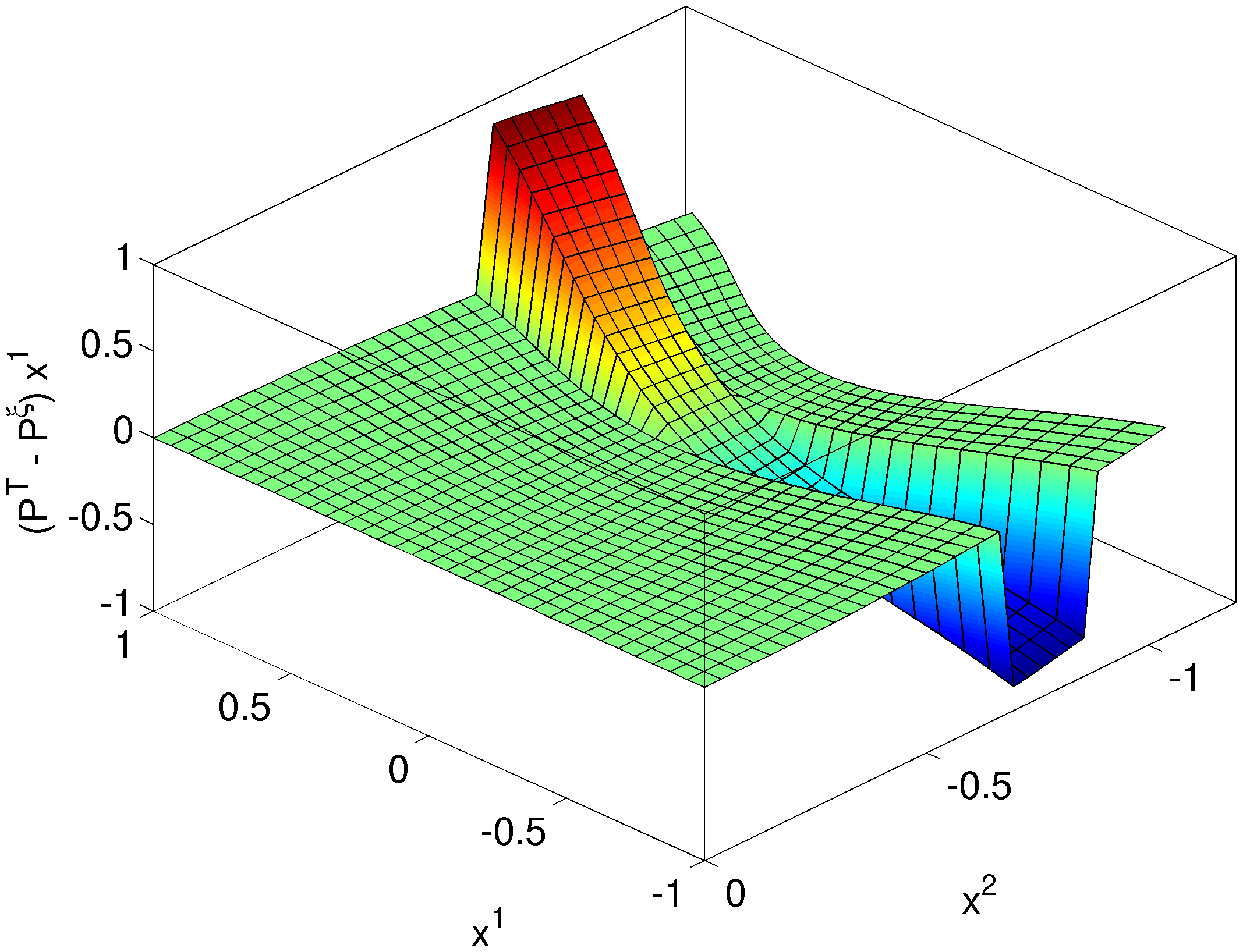
Figure 2: Projection $(x^{1})^{\xi}_{\perp}=(x^{1})^{T}-(x^{1})^{\xi}$, $T=1$, $\xi=0.75$, and $c(x)$ from Section 6.1.

It represents the image of function as a collection of amplitudes of the wave jumps, which pass through the medium and are observed on the screen: see Fig. 2.

Let $\{f_{\alpha}^{T}\}$ and $\{f_{\alpha}^{\xi}\}$ be the control families, which are complete in $\mathcal{F}^{T}_{\sigma}$ and $\mathcal{F}^{T,\xi}_{\sigma}$ respectively, $\{u_{\alpha}^{T}\}$ and $\{u_{\alpha}^{\xi}\}$ the corresponding wave bases in $\mathcal{H}^{T}_{\sigma}$ and $\mathcal{H}^{\xi}_{\sigma}$. The controllability property enables one to represent the truncated functions by (25)

$$y^{T}\,=\,\lim_{N\to\infty}\sum\limits_{\alpha=1}^{N}c^{T,\,N}_{\alpha}\,u^{T}_{\alpha}\,,\qquad y^{\xi}\,=\,\lim_{N\to\infty}\sum\limits_{\alpha=1}^{N}c^{\xi,\,N}_{\alpha}\,u^{\xi}_{\alpha}$$ (36)

with the coefficients determined by the linear systems (26). Substituting the expansions (36) for $y^{T}$ and $y^{\xi}$ to (35), we easily get

$$\tilde{y}(\gamma,\xi)=\left[\lim_{N\to\infty}\sum\limits_{\alpha=1}^{N}\,\left(c^{T,\,N}_{\alpha}\,O^{T}u^{T}_{\alpha}-c^{\xi,\,N}_{\alpha}\,O^{T}u^{\xi}_{\alpha}\right)\right](\gamma,T-\xi-0)\,.$$

By (24), we have $O^{T}u^{f}=C^{T}f$ and, hence, arrive at the representation

$$\tilde{y}(\gamma,\xi)=\left[\lim_{N\to\infty}\sum\limits_{\alpha=1}^{N}\,\left(c^{T,\,N}_{\alpha}\,C^{T}f^{T}_{\alpha}-c^{\xi,\,N}_{\alpha}\,C^{T}f^{\xi}_{\alpha}\right)\right](\gamma,T-\xi-0),\qquad(\gamma,\xi)\in\Sigma^{T}_{\sigma},$$

which is called an amplitude formula (AF). It is the relation, which is the main computational device of the BCM.

4.4 Visualizing waves and harmonic functions

Take a control $f\in\mathcal{F}^{T}$. The wave $u^{f}$ has the part $u^{f}(\cdot,T)\big{|}_{B^{T}_{\sigma}}$, which is a function on the tube. Such a function has an image on the screen $\Sigma^{T}_{\sigma}$. For this image the amplitude formula provides

$$\widetilde{\left[u^{f}(\cdot,T)\right]}(\gamma,\xi)\,=\left[\lim_{N\to\infty}\sum\limits_{\alpha=1}^{N}\,\left(c^{T,\,N}_{\alpha}\,C^{T}f^{T}_{\alpha}-c^{\xi,\,N}_{\alpha}\,C^{T}f^{\xi}_{\alpha}\right)\right](\gamma,T-\xi-0),$$ (37)

where $(\gamma,\xi)\in\Sigma^{T}_{\sigma}$ and the coefficients satisfy the linear systems of the form (26)

$$\sum\limits_{\alpha=1}^{N}A^{s}_{\beta\alpha}c^{s,N}_{\alpha}\,=\,b^{s}_{\beta},\qquad\beta=1,\dots N,\qquad s=T,\,\xi$$ (38)

with the matrices

$$A^{s}_{\alpha\beta}\overset{(\ref{Gram general})}{=}\int\limits_{\Sigma^{T}_{\sigma}}\mathrm{d}t\,\mathrm{d}\Gamma\,\left[\left(R^{2T}F^{s}_{\alpha}\right)(\gamma,t)-\left(R^{2T}F^{s}_{\alpha}\right)(\gamma,2T-t)\right]\,f^{s}_{\beta}(\gamma,t)$$ (39)

and the right hand sides

$$b^{s}_{\beta}\,=\,\left(u^{f}(\cdot,T),u^{s}_{\beta}\right)_{\mathcal{H}}\overset{(\ref{Gram general})}{=}\int\limits_{\Sigma^{T}_{\sigma}}\mathrm{d}t\,\mathrm{d}\Gamma\,\left[\left(R^{2T}F^{s}_{\beta}\right)(\gamma,t)-\left(R^{2T}F^{s}_{\beta}\right)(\gamma,2T-t)\right]\,f(\gamma,t)\,.$$ (40)

Now, let a function $a=a(x)$ satisfy $\Delta a=0$ in $\Omega$ and $a\big{|}_{B^{T}_{\sigma}}$ be its part in the tube. Then the amplitude formula provides

$$\tilde{a}(\gamma,\xi)\,=\,\left[\lim_{N\to\infty}\sum\limits_{\alpha=1}^{N}\,\left(c^{T,\,N}_{\alpha}\,C^{T}f^{T}_{\alpha}-c^{\xi,\,N}_{\alpha}\,C^{T}f^{\xi}_{\alpha}\right)\right](\gamma,T-\xi-0),$$ (41)

where $(\gamma,\xi)\in\Sigma^{T}_{\sigma}$ and the coefficients satisfy the linear systems (38) with the same matrices $A^{s}_{\alpha\beta}$ given by (39) but the right hand sides of the form

$$b^{s}_{\beta}\,=\,\left(a,u^{s}_{\beta}\right)_{\mathcal{H}}\overset{(\ref{(a, u^f)})}{=}\,\int\limits_{\Sigma^{T}}\mathrm{d}t\,\mathrm{d}\Gamma\,(T-t)\,\left[a(\gamma)(R^{T}f^{s}_{\beta})(\gamma,t)-\partial_{\nu}a(\gamma)\,f^{s}_{\beta}(\gamma,t)\right]\,.$$ (42)

The external observer applies the controls $f_{\alpha}$ on the boundary part $\sigma$ and measures the response $R^{2T}f_{\alpha}$. As the representations (37)–(42) show, such measurements suffice to recover the images of waves and harmonic functions on the screen $\Sigma^{T}_{\sigma}$. In the BCM such an option is referred to as a visualization.

5 BCM reconstruction

5.1 How BCM works

To recover $c$ in the tube $B^{T}_{\sigma}$ we summarize the previous mathematical considerations to show how the BCM actually works.

A central object of the BCM is the dual dynamic system (19)–(21). It is the acoustic equation with the same speed of sound $c(x)$ as in normal dynamic system (1)–(3) but it is considered in inverted time, with zero Dirichlet boundary conditions on $\Gamma$, with zero initial value of a solution $v^{y}|_{t=T}=0$ at time instance $t=T$, and with some given initial value of time derivative of a solution $\partial_{t}v^{y}|_{t=T}=y(x)$. If the initial data $y(x)$ have a jump discontinuity then well known exact result (34) of geometric optics can be used to relate an amplitude of the jump in normal derivative of the solution $\partial_{\nu}v^{y}|_{\Sigma^{T}}$ with the amplitude of the jump in $y(x)$. Thus, using projections (33) of harmonic functions $(1,x^{1},x^{2},\dots,x^{n})$ on subdomains $\Omega^{\xi}$ filled by waves at different time instances $\xi$ as the discontinuous initial data $y(x)$ we may, by means of measurements of the normal derivative $\partial_{\nu}v^{y}|_{\Sigma^{T}}$ at points on the domain boundary $\Gamma$, extract information about values of the harmonic functions inside the domain $\Omega^{T}$ at points connected by the geodesic lines (acoustic rays) with the observation points on $\Gamma$. In this way the semigeodesic coordinates and hence a speed of sound inside $\Omega^{T}$ can be recovered. The questions are: how to prepare the required discontinuous initial data for the dual dynamic system, and how to calculate the normal derivative of its solution at different times on the boundary $\Gamma$ as only normal dynamic system is at out disposal.

For the first task we make use of the property of approximate controllability of the dynamic system which means that any square-integrable function $y(x)$ can be represented with any prescribed accuracy as a superposition of wave solutions $u^{f_{\alpha}}(\cdot,T)$ produced by some (full) set of boundary controls $f_{\alpha}$. To find the expansion coefficients for the harmonic functions the linear systems (26) have to be solved whose matrix consists of scalar products of the wave solutions and the right hand sides consist of scalar products of the wave solutions and the functions being expanded. The remarkable fact is that all these internal scalar products can be calculated exactly from some external data available on the domain boundary, see the expressions (39) and (42). In the result, by means of the controls $f_{\alpha}$ acting on the boundary we create the required projections of harmonic functions on subdomains $\Omega^{\xi}$ filled by waves at different time instances $\xi$.

For the second task we make use of another remarkable fact. If we take a wave solution produced by a boundary control $f$ as initial value for time derivative $\partial_{t}v^{y}|_{t=T}=y=u^{f}(\cdot,T)$ in the dual dynamic system then normal derivative of the solution $\partial_{\nu}v^{y}|_{\Sigma^{T}}$ can be obtained measuring the response of the normal dynamic system on some double boundary control $F$ related to the control $f$ in a simple manner, see (24) and (16).

Finally, combining together all tricks we come to so called amplitude formula (41) which allows us to calculate the images of harmonic functions in a tube covered by direct rays from measurements of normal derivative of wave solutions produced by some (full) set of boundary controls $f_{\alpha}$ and their double counterparts $F_{\alpha}$.

For a point $x=(x^{1},\dots,x^{n})\in{\bf R}^{n}$, we consider its $k$-th component as a function of $x$ and write $x^{k}(x)$. These coordinate functions are harmonic: $\Delta x^{k}(\cdot)=0$. By $1(\cdot)$ we denote the function equal to $1$ identically; it is also harmonic. All these functions have the images, which can be recovered by the amplitude formula. The following procedure just exploits such an option.

Step 1.   Fix a $\xi<T$. Choose the families of controls $\{f_{\alpha}^{T}\}$ and $\{f_{\alpha}^{\xi}\}$, which are complete in $\mathcal{F}^{T}_{\sigma}$ and $\mathcal{F}^{T,\xi}_{\sigma}$ respectively. Applying (41) and (42), find the images

$$\tilde{x}^{k}(\gamma,\xi)=\beta(\gamma,\xi)x^{k}(x(\gamma,\xi)),\,\,\,k=1,\dots,n;\quad\,\tilde{1}(\gamma,\xi)=\beta(\gamma,\xi)\,.$$

Step 2.  Varying $\xi$, find the images $\tilde{x}^{k}$ on the whole $\Sigma^{T}_{\sigma}$. Thereby, the connection between the ray and Cartesian coordinates is revealed and given by the correspondence:

$$\Sigma^{T}_{\sigma}\ni(\gamma,\xi)\mapsto x(\gamma,\xi)=\left(\frac{\tilde{x}^{1}(\gamma,\xi)}{\tilde{1}(\gamma,\xi)},\dots,\frac{\tilde{x}^{n}(\gamma,\xi)}{\tilde{1}(\gamma,\xi)}\right)\in B^{T}_{\sigma}\,.$$

So, the external observer recovers the tube in $\Omega$.

Step 3.  Differentiation with respect to $\xi$ corresponds to differentiation along the ray in the tube that implies

$$c(x(\gamma,\xi))=\left\{\sum_{k=1}^{n}\left[\frac{\partial{x^{k}\left(x(\gamma,\xi)\right)}}{\partial{\xi}}\right]^{2}\right\}^{\frac{1}{2}},\qquad(\gamma,\xi)\in\Sigma^{T}_{\sigma}\,.$$ (43)

The pairs $\{x(\gamma,\xi),c(x(\gamma,\xi))\}$ for all $(\gamma,\xi)\in\Sigma^{T}_{\sigma}$ constitute the graph of $c$ in $B^{T}_{\sigma}$. Thus, $c|_{B^{T}_{\sigma}}$ is determined.

Remark.   Our procedure recovers the speed of sound in the ray tube, excluding the cut locus. The controls $f_{\alpha}$ prospecting the tube are supported on its bottom $\sigma$ but the response $R^{2T}f_{\alpha}$ has to be measured on a wider part $\Omega^{T}_{\sigma}\cap\Gamma$ of the boundary. There is a version which recovers $c|_{B^{T}_{\sigma}}$ via $R^{2T}f_{\alpha}$ given on $\sigma$ only: see (Belishev et al., 2016), section 4.1. However, it is problematic for numerical implementation.

5.2 Choice of controls

The BCM uses the boundary controls $f_{\alpha}$, which are continuous, vanish at $t=0$, and constitute a complete system in the proper space. We construct a basis of boundary controls by direct product of spatial and temporal bases, $f_{\alpha}(\gamma,t)=\phi_{l}(\gamma)\,\psi_{m}(t)$, $\alpha=l+mN_{\gamma}$, where $l={0:N_{\gamma}-1}$, $m={0:N_{t}-1}$, and the basis dimension is $N=N_{\gamma}N_{t}$.

In case of semiplane we can keep under control only a part of the boundary and thus have to use localized spatial basis functions. The simplest and good choice is conventional trigonometric basis localized to interval [-1, 1] by an exponential cutoff multiplier (Belishev et al., 2016). The commonly used in FEA tent functions are another convenient choice which has several advantages: the simplicity of hardware implementation and the same spatial scale of all basis elements. Moreover, the tent functions are also very suitable for construction of the temporal basis since all basis functions (and corresponding solutions) can be obtained from the first one just by delays in time. However, the tent functions have discontinuous derivative and the rate of convergence of conventional numerical methods for generation of synthetic inverse data is low.

To overcome this difficulty we have used a smooth tent-like function,

$$\theta(z)=\frac{d}{\Delta}\,\ln\left[\frac{\cosh\left(\frac{2\Delta-z}{2d}\right)\cosh\left(\frac{z}{2d}\right)}{\cosh^{2}\left(\frac{\Delta-z}{2d}\right)}\right]/\left[1-\exp\left(-\frac{\Delta}{d}\right)\right],$$

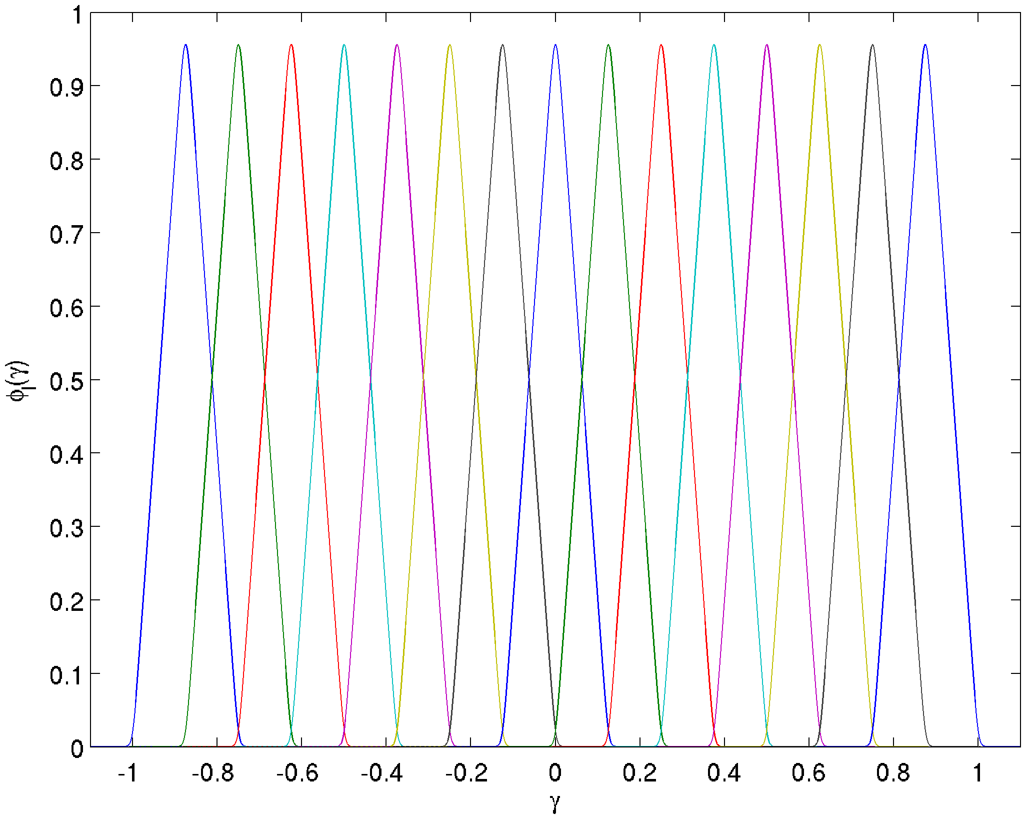
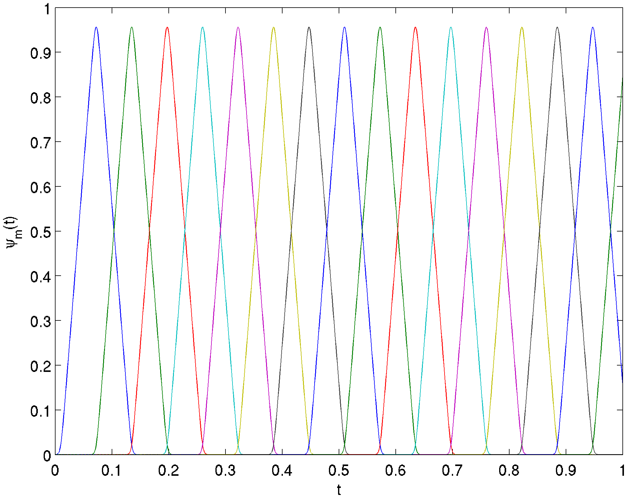
Figure 3: Basis of boundary controls: 15 spatial functions $\phi_{l}(\gamma)$ on interval $[-1,1]$ (top), and 16 temporal functions $\psi_{m}(t)$ on interval $[0,T]$ with $T=1$ (bottom). In both cases $d=\Delta/32$.

where $z$ is an independent variable ($\gamma$ or $t$), $2\Delta$ is the triangle base, and $d$ is a smoothing parameter (when $d\rightarrow 0$ function $\theta(z)$ gets a triangular shape). The spatial functions on interval $\gamma\in[a,b]$ are $\phi_{l}(\gamma)=\theta(\gamma-a-l\Delta)$, where $\Delta=(b-a)/(N_{\gamma}+1)$. The temporal functions on interval $t\in[0,T]$ are $\psi_{m}(t)=\theta(t-\delta-m\Delta)$, where $\Delta=T/N_{t}$, and $\delta$ is a small offset to ensure a negligible value of $\theta(0)$. Such simple and translationally invariant basis shown in Fig. 3 considerably reduces computational resources needed for BCM reconstruction.

5.3 Regularization

In BCM we expand discontinuous projections $a^{\xi}=P^{\xi}a$ over smooth wave solutions $u^{\xi}_{\alpha}(\cdot,T)$ and thus have to observe the Gibbs oscillations. The basis functions have a finite resolution of order of spatial and temporal scales of the tent-like functions. All scales below the minimum ones are unreachable, therefore we average a result of expansion $g(\gamma,t)$ over that minimum scales by convolution with some kernel $K(\gamma,\xi)$,

$$\langle g\rangle(\gamma,t):=\int\limits_{-\infty}^{+\infty}\mathrm{d}t^{\prime}\int\limits_{-\infty}^{+\infty}\mathrm{d}\gamma^{\prime}K(\gamma-\gamma^{\prime},t-t^{\prime})\,g(\gamma^{\prime},t^{\prime}).$$ (44)

In our implementation the kernel $K(\gamma-\gamma^{\prime},t-t^{\prime})$ is a product of conventional Gaussian kernels both for spatial and temporal variables. Such procedure efficiently removes the Gibbs oscillations and thus de facto accelerates convergence of the expansions. The values of standard deviations in Gaussian kernels should match the minimum spatial and temporal scales of the boundary controls to efficiently smooth out the Gibbs oscillations.

Due to unavoidable errors in matrix elements and right hand sides of linear systems, the expansion coefficients $c^{\xi,\,N}_{\alpha}$ also contain errors amplified by ill-conditioned matrix $A$. In some cases we have to use Tikhonov (or other) regularization to reduce additional fake oscillations caused by errors in expansion coefficients. The value of the regularization parameter is selected to satisfy a desired tolerance for residual of the linear systems.

6 Numerical testing

We have performed detailed tests of quality of the BCM reconstruction on semiplane (with trigonometric spatial basis) in (Belishev et al., 2016). The method have demonstrated a good accuracy of reconstruction of $c(x)$ (of order of several percents in most part of the recovered domain) in cases of regular field of acoustic rays.

The goal of the following tests is to try the method with the tent-like spatial basis functions and in case of irregular realistic field of acoustic rays (Marmousi model).

For each delayed control $f^{\xi}_{\alpha}(\gamma,t)$ and its double version $F^{\xi}_{\alpha}(\gamma,t)$, we have to find a solution of the direct problem (1)-(3) and to measure the system’s reaction at the boundary $\Gamma$. For this purpose, we have implemented an universal semidiscrete central-upwind third order accurate numerical scheme with WENO reconstruction suggested in (Kurganov et al., 2001).

The reaction data are then used in the procedure described in Section 5.1 to reconstruct a speed of sound $c(x)$. The procedure is simple and efficient, essentially it involves a calculation of quadratures (double sums) for scalar products and a solution of the resulting linear systems by standard LAPACK routines.

6.1 Case 1

We take a speed of sound $c(x)=\rho(x)^{-\frac{1}{2}}$ produced by the density of medium,

$$\rho(x^{1},x^{2})=1+a\,g_{1}(x^{1})\,g_{2}(x^{2}),$$

$$\quad g_{k}(x^{k})=\exp{\left[-\frac{\left(x^{k}-\bar{x}^{k}\right)^{2}}{2\Delta_{k}^{2}}\right]},$$

where $a=1$, $\bar{x}^{1}=0$, $\bar{x}^{2}=-0.5$, $\Delta_{1}=0.5$, $\Delta_{2}=0.5$.

The boundary control is applied on a part of the boundary $\gamma\in(-1,1)$ with probing time $T=1$. The field of acoustic rays shown in Fig. 1 is regular in the prospected domain. The basis of controls is composed from $N_{\gamma}=15$ tent-like spatial functions and $N_{t}=16$ tent-like temporal functions. The dimension of each basis is selected to obtain a desired spatial resolution and accuracy of reconstruction.

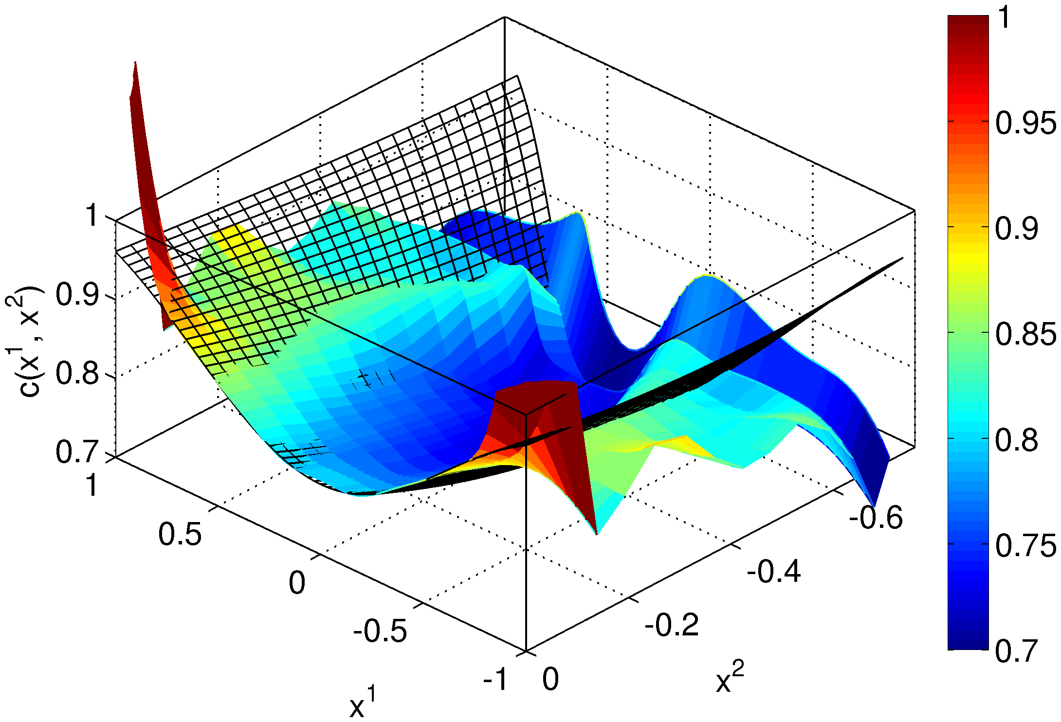
Figure 4: Test 1. Top - exact (mesh) and recovered (surface) values of speed of sound $c(x)$, bottom - map of relative errors (in percents) of the recovered values of $c(x)$ in cartesian coordinates.

The exact and recovered values of speed of sound $c(x)$ are shown in the top panel of Fig. 4 while the relative errors of reconstruction are shown in the bottom panel of the figure. The parameter of Tikhonov regularization for all linear systems is $\varepsilon=1{\cdot}10^{-6}$, and standard deviations of Gaussian kernels in (44) for $(\gamma,t)$ are $\sigma_{\gamma}=0.125$ and $\sigma_{t}=0.0625$. We observe that in most part of the domain covered by direct rays from the active boundary interval $\sigma$ the relative error does not exceed a few percents. However, as expected, the reconstruction error grows towards the lateral borders of the recovered domain and for large values of $\xi\approx T$. This is the effect of degraded quality of harmonic functions projections produced by controls acting from the boundary.

6.2 Case 2

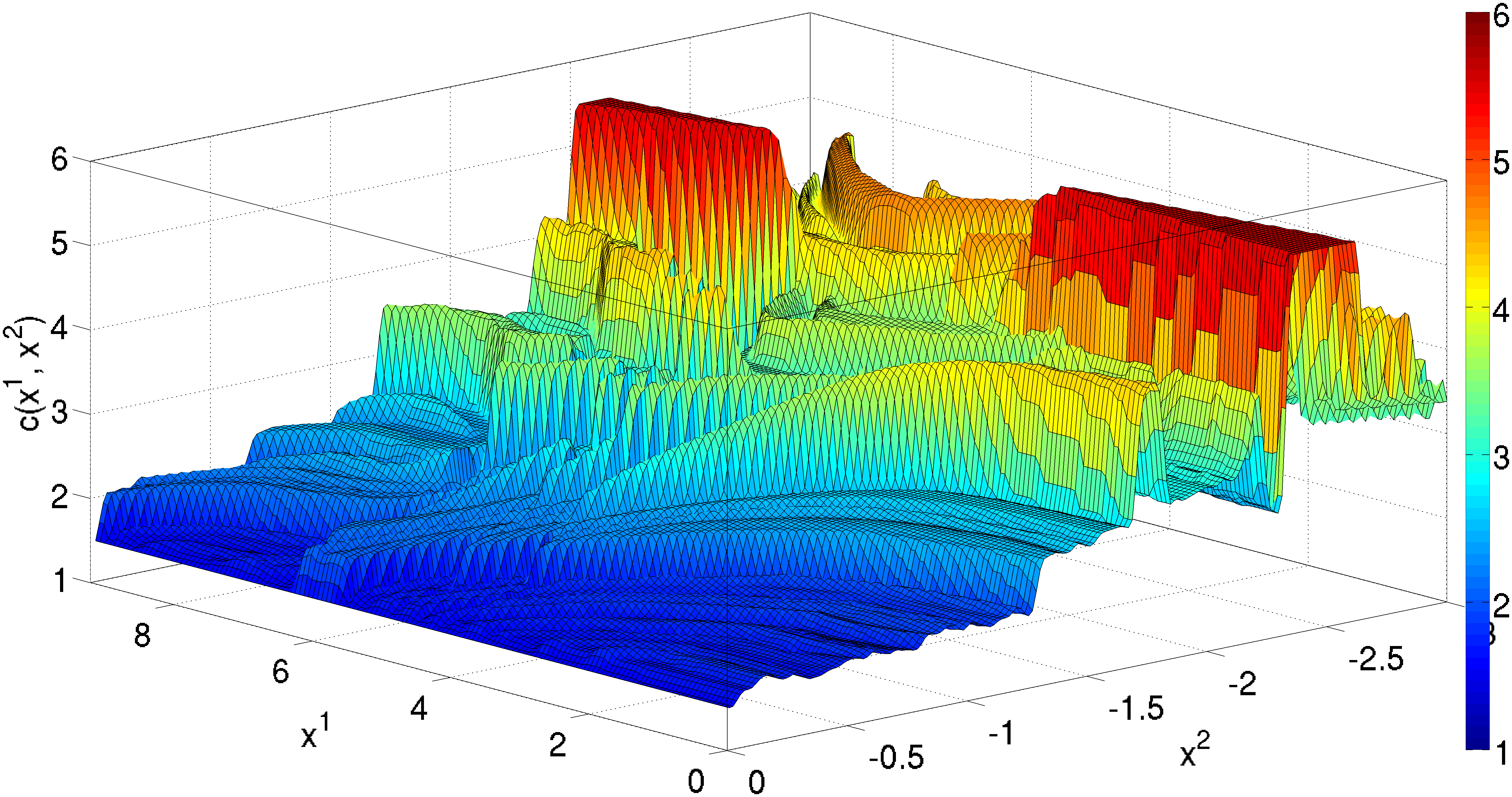
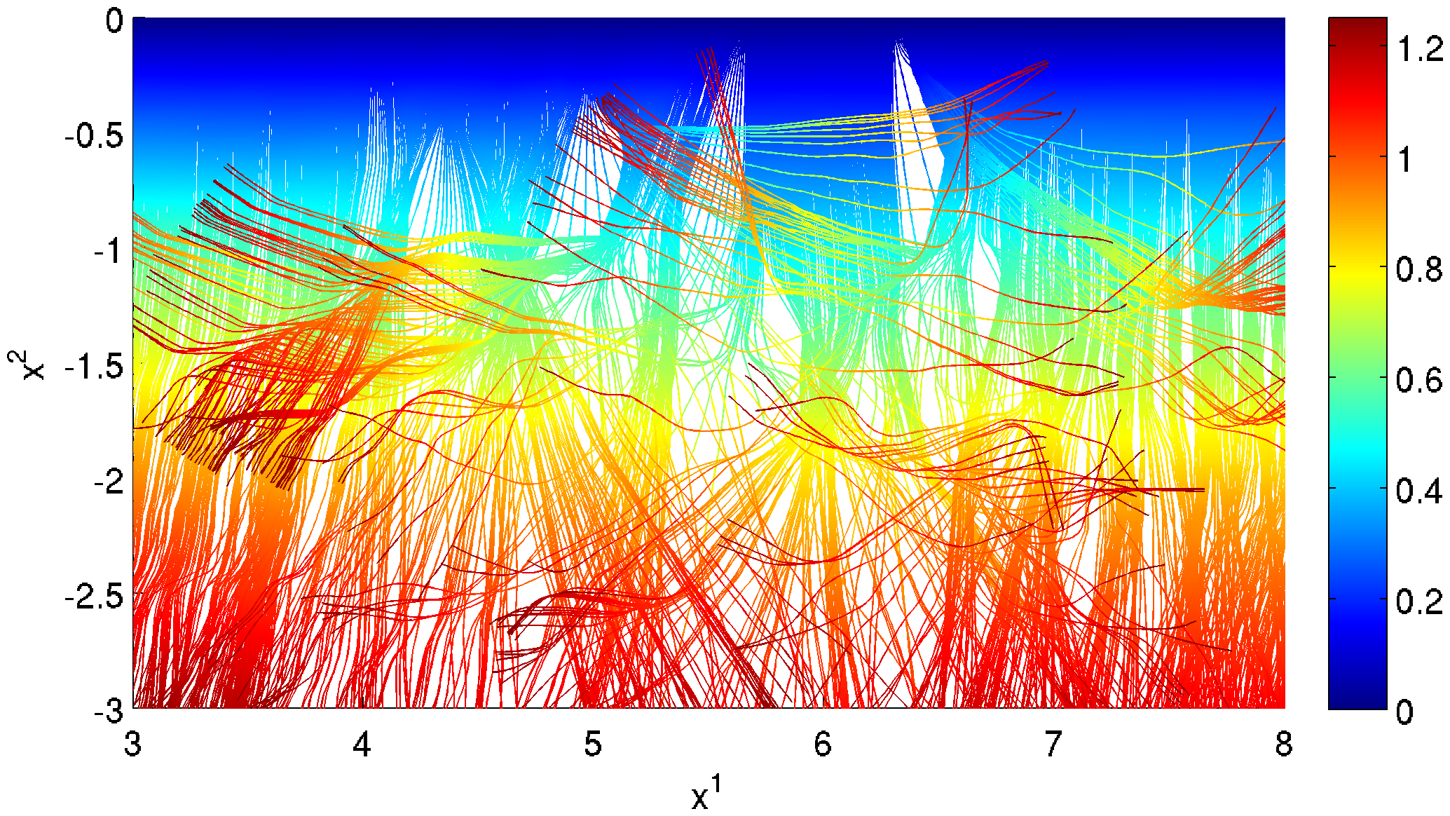
Figure 5: Test 2. Top - speed of sound in the smoothed Marmousi model, bottom - field of acoustic rays $x(\gamma,\xi)$ emanating orthogonally from $\sigma$ with probing time $T=1.25$ s.

For the second test we have selected a speed of sound from famous Marmousi model which has extremely complicated and irregular field of acoustic rays, see the bottom panel of Fig. 5. The original discontinuous and spiky Marmousi speed data were slightly smoothed out by convolution with a short scale bump kernel for better accuracy of numerical simulations of inverse data. We also smoothly extended the original speed of sound to a larger spatial domain to test the BCM reconstruction on the whole domain with Marmousi data. The resulting speed of sound (without the extension) is shown in the top panel of Fig. 5. The Marmousi density data were not used in our one-parameter acoustic equation.

The boundary control is done on a part of the boundary $\gamma\in(0,9.2)$ km with probing time $T=1.25$ s which is enough to prospect the domain up to $3$ km below the boundary. The basis of controls is composed from $N_{\gamma}=31$ tent-like spatial functions and $N_{t}=32$ tent-like temporal functions. The standard deviations of Gaussian kernels are $\sigma_{\gamma}=0.2875$ km and $\sigma_{t}=0.0390625$ s.

It is obvious that resolution of the given basis is not enough to reconstruct sharp features of Marmousi model. As expected, in such case the BCM procedure recovers an averaged profile of the speed of sound, see the top panels of Fig. 6 and Fig. 7. To understand the reason of large reconstruction errors at depths with $x^{2}<-2$ km we also performed so called pseudo-reconstruction, see the bottom panels of Fig. 6 and Fig. 7. It means the same reconstruction procedure of Section 5.1 but with all scalar products (in linear systems) evaluated by more accurate internal quadratures (11) instead of external ones (10). We see that pseudo-reconstruction has a similar accuracy at small to moderate depths but it is much more accurate at large depths. This can be explained as follows. The condition number of matrices $A^{\xi}$ (39) grows as $\xi^{4}$, and it reaches values of order $10^{5}-10^{6}$ at $\xi\sim T$. The errors of the expansion coefficients $c^{\xi,\,N}$ are the errors of the right hand sides $b^{\xi}$ multiplied on the condition number of $A^{\xi}$. For large depths of recovering the accuracy of external scalar products is not enough to provide accurate values of expansion coefficients and (after all reconstruction steps) speed of sound.

The relative errors of the recovered speed of sound are shown in Fig. 8. We see that in the most part of the prospected domain the relative errors do not exceed $10-15\%$. The BCM procedure provides a reasonable accuracy even for extremely irregular field of acoustic rays.

7 Conclusion

In the present work we have investigated practical capabilities of the Boundary Control Method applied to acoustic equation on semiplane. This ab initio and direct reconstruction method does not require any a priory information about the recovered parameters of a dynamic system. To solve inverse problem, the BCM exploits subtle and rigorous properties of the dynamic system.

The BCM reconstruction procedure is simple and efficient, essentially it involves calculation of quadratures for matrix elements (double sums) and solving linear systems by standard LAPACK routines. The method may require additional regularization (e.g. by Tikhonov) of the linear systems and smoothing (e.g. by convolution with some kernel) of the Gibbs oscillations arising in expansions of projections of harmonic functions over wave solutions. The preparation of synthetic inverse data for BCM is rather CPU time consuming since we have to solve the direct problem for $2^{8}-2^{12}$ boundary controls with a good accuracy.

The condition number of matrices $A^{\xi}$ composed from scalar products of wave solutions produced by set of boundary controls quickly grows with the probing time $\xi\in[0,T]$. This effect is manifestation of ill-posedness of the inverse problem and it imposes a practical limit on the maximum depth of reconstruction of speed of sound. To increase the depth of reconstruction we have to reduce errors in system’s reaction data and/or decrease the number of active boundary controls (the matrix dimension). The use of sliding support $\sigma$ allows to decrease the number of boundary controls without degradation of spatial resolution of the basis.

The application of BCM to realistic model of speed of sound by Marmousi has confirmed that the method is able to work in cases with extremely complicated and irregular field of acoustic rays.

The number and shape of boundary controls determine the spatial resolution of the reconstruction procedure. The BCM demonstrates ability to work with low number of boundary controls – in such case it recovers an ‘averaged’ profile that can be further used as a ‘zero order’ starting approximation for high resolution iterative reconstruction methods.

8 Acknowledgments

I. B. I. was greatly supported by his wife and partly by Volks-Wagen Foundation. M. I. B. was supported by the grant RFBR 14-01-00535A and by Volks-Wagen Foundation. All authors acknowledge partial support within the contract 2-53-04-SKIF/NIR/16-SPbSU.

9 Figures

Figure 6: Test 2. The speed of sound in Marmousi model: top - normal reconstruction (${\epsilon=1\cdot 10^{-5}}$), bottom - pseudo-reconstruction (${\epsilon=5\cdot 10^{-7}}$). The exact values of $c(x)$ in both panels are shown by mesh.

Figure 7: Test 2. The profiles of speed of sound in Marmousi model: top - normal reconstruction (${\epsilon=1\cdot 10^{-5}}$), bottom - pseudo-reconstruction (${\epsilon=5\cdot 10^{-7}}$). The exact values are shown by solid lines, the recovered values are shown by dots.

Figure 8: Test 2. The map of relative errors of speed of sound in percents: top - normal reconstruction (${\epsilon=1\cdot 10^{-5}}$), bottom - pseudo-reconstruction (${\epsilon=5\cdot 10^{-7}}$).

References

- Avdonin and Belishev (2005) S. A. Avdonin and M. I. Belishev. Dynamical inverse problem for the shrödinger equation (the bc-method). Amer. Math. Soc. Transl. Ser., 2:214, 2005.
- Babich and Buldyrev (1991) V. M. Babich and V. S. Buldyrev. Short Wave Length Diffraction Theory (Asymptotic Methods). Heidelberg: Springer, 1991.
- Belina and Klibanov (2008) L. Belina and M. V. Klibanov. A globally convergent numerical method for a coefficient inverse problem. SIAM J. Sci. Comp., 31:478–509, 2008.
- Belina and Klibanov (2012) L. Belina and M. V. Klibanov. Approximate Global Convergence and Adaptivity for Coefficient Inverse Problems. Springer, 2012.
- Belishev (1988) M. I. Belishev. An approach to multidimensional inverse problems for the wave equation. Sov. Math. Dokl., 36:481–484, 1988.
- Belishev (1997) M. I. Belishev. Boundary control in reconstruction of manifolds and metrics. Inverse Problems, 13:R1–R45, 1997.
- Belishev (2007) M. I. Belishev. Recent progress in the boundary control method. Inverse Problems, 23:R1–R67, 2007.
- Belishev and Demchenko (2011) M. I. Belishev and M. N. Demchenko. Time-optimal reconstruction of riemannian manifold via boundary electromagnetic measurements. J. Inverse Ill-Posed Probl., 19(2):167–188, 2011.
- Belishev and Glasman (2001) M. I. Belishev and A. K. Glasman. Dynamical inverse problem for the maxwell system: recovering the velocity in a regular zone (the bc-method). St Petersburg Math. J., 12:279–316, 2001.
- Belishev and Gotlib (1999) M. I. Belishev and V. Y. Gotlib. Dynamical variant of the bc-method: theory and numerical testing. J. Inverse Ill-Posed Probl., 7(3):221–240, 1999.
- Belishev and Ivanov (2005) M. I. Belishev and S. A. Ivanov. Recovering the parameters of the system of the connected beams from the dynamical boundary data. Zapiski Nauch. Semin. POMI., 324:20–42, 2005.
- Belishev and Mikhailov (2014) M. I. Belishev and V. S. Mikhailov. Inverse problem for a one-dimensional dynamical dirac system (bc-method). Inverse Problems, 30(12):125013, 2014.
- Belishev and Vakulenko (2006) M. I. Belishev and A. F. Vakulenko. Inverse problems on graphs: recovering the tree of strings by the bc-method. J. Inverse Ill-Posed Probl., 14(1):29–46, 2006.
- Belishev et al. (1997) M. I. Belishev, V. Y. Gotlib, and S. A. Ivanov. The bc-method in multidimensional spectral inverse problem: theory and numerical illustrations. ESAIM Control Optim. Calc. Var., 2:307–327, 1997.
- Belishev et al. (2016) M. I. Belishev, I. B. Ivanov, I. V. Kubyshkin, and V. S. Semenov. Numerical testing in determination of sound speed from a part of boundary by the bc-method. J. of Inv. and Ill-posed Probl., 23(5), 2016.
- Kabanikhin and Shishlenin (2004) S. I. Kabanikhin and M. A. Shishlenin. Boundary control and gel’fand-levitan-krein methods in inverse acoustic problem. J. Inverse Ill-Posed Probl., 12(2):125–144, 2004.
- Kabanikhin and Shishlenin (2011) S. I. Kabanikhin and M. A. Shishlenin. Numerical algorithm for two-dimensional inverse acoustic problem based on gel’fand-levitan-krein equation. J. Inverse Ill-Posed Probl., 18(9):979–995, 2011.
- Kabanikhin et al. (2005) S. I. Kabanikhin, A. D. Satybaev, and M. A. Shishlenin. Direct Methods of Solving Multidimensional Inverse Hyperbolic Problems. VSP, 2005.
- Kurganov et al. (2001) A. Kurganov, S. Noelle, and G. Petrova. Semidiscrete central-upwind schemes for hyperbolic conservation laws and hamilton–jacobi equations. SIAM Journal on Scientific Computing, 23(3):707–740, 2001.
- Oksanen (2013) L. Oksanen. Solving an inverse obstacle problem for the wave equation by using the boundary control method. Inverse Problems, 29(3):035004, 2013.
- Pestov et al. (2010) L. Pestov, V. Bolgova, and O. Kazarina. Numerical recovering of a density by the bc-method. Inverse Probl. and Imaging, 4(4):701–712, 2010.
- Pestov et al. (2012) L. Pestov, V. Bolgova, and A. Danilin. Numerical recovering of a speed of sound by the bc-method in 3d. In Acoustical Imaging, volume 31 of Acoustical Imaging, pages 201–209. 2012.
- Pestov (2012) L. N. Pestov. Inverse problem of determining absorption coefficient in the wave equation by bc method. J. Inverse Ill-Posed Probl., 20(1):103–110, 2012.
- Pestov (2014) L. N. Pestov. On determining an absorption coefficient and a speed of sound in the wave equation by the bc method. J. Inverse Ill-Posed Probl., 22(2):245–250, 2014.
- Romanov (1996) V. G. Romanov. A local version of a numerical method for solving an inverse problem. Siberian Math. J., 37(4):797–810, 1996.