Discrete Sums of Geometric Brownian Motions, Annuities and Asian Options

Abstract.

The discrete sum of geometric Brownian motions plays an important role in modeling stochastic annuities in insurance. It also plays a pivotal role in the pricing of Asian options in mathematical finance. In this paper, we study the probability distributions of the infinite sum of geometric Brownian motions, the sum of geometric Brownian motions with geometric stopping time, and the finite sum of the geometric Brownian motions. These results are extended to the discrete sum of the exponential Lévy process. We derive tail asymptotics and compute numerically the asymptotic distribution function. We compare the results against the known results for the continuous time integral of the geometric Brownian motion up to an exponentially distributed time. The results are illustrated with numerical examples for life annuities with discrete payments, and Asian options.

1. Introduction

The valuation and risk management of annuities are important topics in the actuarial science. There is a wide variety of contractual annuity payoffs, ranging from fixed payouts to variable annuities, possibly with guaranteed benefits features. The pricing and valuation of such contracts have been considered in the actuarial literature, under different choices of equity price, mortality and interest rate models [18, 25, 35, 10, 33]. Most of the theoretical work on variable annuities in the literature is in a continuous-time setting, although in practice these instruments are defined and simulated in discrete time. We note that discrete time models have been also considered in the actuarial literature [21]. In this paper we will work in a discrete time setting, and will compare our results with the continuous time approximation.

We will consider in this paper the case of a fixed payout annuity under the geometric Brownian motion model for the equity returns. The interest rates will be assumed to be constant and deterministic, and the mortality will be described by a geometric distribution. This setting is of interest both from a theoretical point of view, and as a simple starting point for building more complicated and realistic models. The geometric Brownian motion model for equities prices (the Black-Scholes model) is the simplest model available in the literature. The lognormal model (Independent Lognormal ILN) is also one of the recommended models in the American Academy of Actuaries report, and is used for generating pre-packaged economic scenarios (see [2], Appendix 2.). This model can be extended by adding stochastic volatility, modeled either as a diffusion or using a regime-switching approach.

Under the lognormal returns equity model, the present value of a fixed coupon annuity can be related to the sum of geometric Brownian motions (GBM) sampled on a discrete time points. The distributional properties of this quantity, both in a discrete and continuous time setting, have been widely studied in the mathematical finance and actuarial literature, see [13, 15] for overviews. Consider for example a stochastic annuity which pays a constant coupon $C$ at regular times with time step size $\tau$. Furthermore, assume that the payments are made from a portfolio containing an asset with value process $U_{t}$ which is stochastic and follows a geometric Brownian motion:

(1) $$U_{t}=e^{\sigma W_{t}+(m-\frac{1}{2}\sigma^{2})t},$$

where $W_{t}$ is a standard Brownian motion starting from $0$ at time $0$, and $\sigma,m$ are real parameters. $U_{t}$ represents the value at time $t$ of one unit of currency invested at time zero into the asset (for example stocks), which has normally distributed log-returns.

The present value of the annuity, assumed to pay $n$ coupons at times $t_{i}$, is

(2) $$S_{n}=\sum_{i=1}^{n}D_{t_{i}}\frac{C}{U_{t_{i}}},$$

where $D_{t_{i}}$ are discount factors. This quantity is a random variable and represents the liability, or amount of currency required at time zero in order to be able to pay the annuity cash flows. We are interested in the shape of the probability density of $S_{n}$, and especially in the tails of this distribution, which give the probabilities of extreme values of the liability represented by the annuity payments. If the discounting rate $r$ is constant and deterministic, the discount factors are exponential $D_{t_{i}}=e^{-rt_{i}}$ and the annuity value $S_{n}$ is proportional to the sum of a geometric Brownian motion sampled on discrete times $t_{i}$

(3) $$\tilde{S}_{n}=\sum_{i=1}^{n}e^{-\sigma W_{t_{i}}+(\frac{1}{2}\sigma^{2}-m)t_{i}},$$

where we redefined $m+r\to m$.

A related quantity appears in the problem of pricing Asian options with discrete sampling, which are derivatives linked to the average of the price of an asset $S_{t}$

(4) $$A_{n}=\frac{1}{n}\sum_{i=1}^{n}S_{t_{i}},$$

under the assumption that $S_{t}$ follows a geometric Brownian motion

(5) $$S_{t}=S_{0}e^{\sigma W_{t}+(m-\frac{1}{2}\sigma^{2})t}.$$

Here $W_{t}$ is a standard Brownian motion, and $\sigma,m$ are the volatility and drift of the asset.

If the averaging times are uniformly distributed and the time step is sufficiently small, the time average (4) can be approximated by the continuous time average

(6) $$A_{n}=\frac{1}{t_{n}}\int_{0}^{t_{n}}S_{t}dt\,.$$

This reduces the problem to the study of the distributional properties of the time integral of the geometric Brownian motion, which has been extensively studied in the literature [12, 13, 40, 41].

The distributional properties of the time-integral of the geometric Brownian motion simplify very much in the infinitely large time limit. Define

(7) $$Y_{T}=\int_{0}^{T}dte^{\sigma W_{t}+(m-\frac{1}{2}\sigma^{2})t}.$$

The following result was proven in [12], see Section 3 in [16] for a survey of related results.

Theorem 1 ([12, 16]).

The limit $\lim_{T\to\infty}Y_{T}=Y_{\infty}$ exists in distribution if and only if $m-\frac{1}{2}\sigma^{2}<0$, and,

(8) $$\frac{2}{\sigma^{2}Y_{\infty}}=\mathbf{Gamma}\left(1-\frac{2m}{\sigma^{2}},1\right)\,.$$

The limit probability density of $Y_{\infty}$ is given by the inverse Gamma distribution. The probability density function $\mathbb{P}(Y_{\infty}\in(z,z+dz))=\phi_{\infty}(z)dz$, is given by

(9) $$\phi_{\infty}(z;\sigma,m)=\left(\frac{2}{\sigma^{2}}\right)^{1-\frac{2m}{\sigma^{2}}}\left(\frac{1}{z^{2}}\right)^{1-\frac{m}{\sigma^{2}}}\frac{1}{\Gamma\left(1-\frac{2m}{\sigma^{2}}\right)}\exp\left(-\frac{2}{\sigma^{2}z}\right)\,.$$

The cumulative distribution is

(10) $$\Phi_{\infty}(x;\sigma,m)=\mathbb{P}(Y_{\infty}<x)=\frac{1}{\Gamma\left(1-\frac{2m}{\sigma^{2}}\right)}\Gamma\left(1-\frac{2m}{\sigma^{2}};\frac{2}{\sigma^{2}x}\right),$$

where $\Gamma(a,x)=\int_{x}^{\infty}t^{a-1}e^{-t}dt$ is the incomplete Gamma function.

We study in this paper the distributional properties of the discrete sum of the GBM sampled on uniformly spaced times $t_{i}=i\tau$

(11) $$X_{n}=\sum_{i=1}^{n}e^{\sigma W_{t_{i}}+(m-\frac{1}{2}\sigma^{2})t_{i}}.$$

The sum of the inverse of the GBM (3) can be obtained from this by replacing $\sigma\to-\sigma,m\to-m+\sigma^{2}$. We will study the distributional properties of $X_{n}$, of the infinite sum of GBM $X_{\infty}=\lim_{n\to\infty}X_{n}$, and of $X_{N}$, the sum of GBM with geometrically distributed $N$. We study the existence of the $n\to\infty$ limit, the tail asymptotics for all three cases, and the moments of the corresponding random variables, and also the convergence of the discrete sums to the continuous time integrals. The results will then be applied to study annuities and Asian options. We also also illustrate our results numerically.

The problem of determining the distribution of the discrete sum of GBM is closely related to the study of the distribution of the sum of log-normals which has a long history, see [3] for a literature overview. The simplest approach is to approximate the distribution with a log-normal random variable [27, 16]. The tails asymptotics of the sum of correlated log-normals has been studied in [4, 19, 24]. Dufresne [16] studied the distribution of the sum (11), generalized by the introduction of an weight function, in the small volatility limit $\sigma\to 0$, and derived a limit theorem for this quantity.

Milevsky and Posner [31] studied the pricing of Asian options with discrete monitoring. They applied the distributional properties of the infinite time integral of the GBM to the discrete sum $X_{n}$, and proposed to use the inverse Gamma distribution as an approximation for the finite sum, as a parametric approximation for pricing Asian options. The inverse Gamma distribution is obtained only for continuous time; in discrete time the distribution is different, and we study here the corrections to the approximation of the discrete infinite sum with the continuous time integral.

The present authors [29] studied the distributional properties of the sum (11) in the $n\to\infty$ limit at fixed $\beta=\frac{1}{2}\sigma^{2}\tau n^{2}$, and found almost sure limit, fluctuations and large deviations of the average $A_{n}=\frac{1}{n}X_{n}$ and then obtained the asymptotics for the prices of out-of-the-money, in-the-money and at-the-money Asian options. Notice that the fixed $\beta$ and $n\rightarrow\infty$ limit corresponds to the small maturity or small volatility regimes. For Asian options, the typical maturity can be $1$ year or $2$ year and the volatility is usually less than $100\%$. Thus the small maturity or small volatility regimes are of practical interest in business applications. The case of fixed $\sigma,\tau$ and $n\rightarrow\infty$ gives the infinite sum of geometric Brownian motions $X_{\infty}$. This situation corresponds to the large maturity or large time-horizon regime, which are of practical interest for stochastic annuities, but less relevant for the pricing of Asian options.

The paper is organized as follows. In Section 2, we study the properties of the distribution of the infinite sum of a geometric Brownian motion. We obtain a stochastic recurrence equation and use it to derive an integral equation for the probability density function of the infinite sum of the geometric Brownian motion $X_{\infty}$ sampled on a uniformly spaced time grid with time step $\tau$. We derive the right and left tail asymptotics for $X_{\infty}$. As the time step goes to zero $\tau\to 0$, we show that the infinite sum of geometric Brownian motions converges in $L^{1}$ norm to the infinite integral, which is known to follow an inverse Gamma distribution [12], see Theorem 1. In Section 3, we repeat the analysis for the sum of geometric Brownian motions stopped at a geometric stopping time. In the context of the stochastic annuities, this corresponds to a geometrically distributed mortality time. As the time step goes to zero, we show that this sum converges in distribution to the continuous time integral of geometric Brownian motion with exponentially distributed terminal time, whose properties are well understood in the literature. In Section 4, we extend the results for the sums of geometric Brownian motions to the sums of exponential Lévy processes, and in Section 5, we derive explicit expressions for the positive moments of the infinite sum of GBM. In Section 6, we apply our results to study annuities with finite mortality, stochastic mortality and the risk measures of the annuities, including the Value-at-Risk, and also the pricing of discrete time Asian options. We conclude the paper with numerical illustrations of the results in Section 7.

2. Infinite Sum of the GBM

We study in this section the infinite sum of GBM $X_{\infty}=\lim_{n\to\infty}X_{n}$, where $X_{n}$ is defined in (11). The density of this random variable satisfies a functional relation, given by the following result.

Proposition 2.

The infinite sum of GBM $X_{\infty}$, if exists, satisfies the relation

(12) $$X_{\infty}=\mathcal{A}(1+X_{\infty}),$$

where the equality is in distribution, and we denoted

(13) $$\mathcal{A}:=e^{\sigma\sqrt{\tau}Z+(m-\frac{1}{2}\sigma^{2})\tau},$$

with $Z\sim N(0,1)$ independent of $X_{\infty}$.

Proof.

The infinite sum of GBM, if exists, can be written as the sum of products of i.i.d. factors of the form (13)

(14) $$X_{\infty}=\mathcal{A}_{1}+\mathcal{A}_{1}\mathcal{A}_{2}+\mathcal{A}_{1}\mathcal{A}_{2}\mathcal{A}_{3}+\cdots=\mathcal{A}_{1}(1+\mathcal{A}_{2}+\mathcal{A}_{2}\mathcal{A}_{3}+\cdots)=\mathcal{A}_{1}(1+X_{\infty}),$$

where the last equality is in distribution. Since $\mathcal{A}_{i}$ are i.i.d., $\mathcal{A}_{1}$ is independent of $(1+\mathcal{A}_{2}+\mathcal{A}_{2}\mathcal{A}_{3}+\cdots)$ and hence $\mathcal{A}$ is independent of $X_{\infty}$ in (12). ∎

Remark 3.

An easier way to understand (12) is by writing (12) as $X_{\infty}=\mathcal{A}(1+\hat{X}_{\infty})$ in distribution, where $X_{\infty}=\hat{X}_{\infty}$ in distribution and $\mathcal{A}$ is independent of $\hat{X}_{\infty}$.

We study now the existence and uniqueness of the solution of the functional relation (12). This can be related to the existence of a limit distribution for the linear recursion

(15) $$x_{i+1}=a_{i}x_{i}+b_{i}$$

where $(a_{i},b_{i})$ is an i.i.d. pair of random variables with values in $[0,\infty)\times\mathbb{R}$. This reduces to the functional relation (12) by taking $a_{i}=b_{i}=\mathcal{A}$.

Linear random recursions of the form (15) have been widely studied in the probability literature [26, 38, 17, 28, 30]. Explicit solutions for the limit distribution in particular cases have been found in [1, 12, 17, 23, 22].

The conditions for the existence and uniqueness of the limit distribution of the recursion (15) are well-known [26, 38]. The following are sufficient conditions for the existence and uniqueness of the limit distribution

(16) $$\mathbb{E}[\log a_{i}]<0\,,\qquad\mathbb{E}[\log(b_{i})_{+}]<\infty\,.$$

This gives us the following result.

Proposition 4.

The functional relation (12) has a solution, which is furthermore unique, provided that the following inequality holds

(17) $$m<\frac{1}{2}\sigma^{2}.$$

Proof.

The first condition (16) gives

(18) $$\mathbb{E}[\log\mathcal{A}]=\left(m-\frac{1}{2}\sigma^{2}\right)\tau<0\,,$$

which is satisfied for $m<\frac{1}{2}\sigma^{2}$. The second condition (16) is always satisfied.

We conclude that the functional relation (12) has a solution which is furthermore unique, provided that the inequality (17) holds. We note also that the condition under which this result holds is the same as that in the Theorem 1 for the continuous time case. ∎

The relation (12) gives an integral equation for the probability density function of $X_{\infty}$, defined as $\mathbb{P}(X_{\infty}\in(x,x+dx))=f(x;\beta,\rho)dx$. We will show that the probability density function of $X_{\infty}$ depends only on the parameters

(19) $$\beta:=\sigma^{2}\tau\,,\qquad\rho:=m\tau\,.$$

Proposition 5.

The function $f(x;\beta,\rho)$ satisfies the integral equation

(20) $$f(x;\beta,\rho)=\frac{1}{x}\int_{0}^{\infty}\frac{dy}{\sqrt{2\pi\beta}}\exp\left(-\frac{1}{2\beta}\left[\log\left(\frac{x}{1+y}\right)+\frac{1}{2}\beta-\rho\right]^{2}\right)f(y;\beta,\rho)\,.$$

Proof.

For any $x>0$,

(21) $$\mathbb{P}(X_{\infty}\leq x)=\mathbb{P}(\mathcal{A}(1+X_{\infty})\leq x)=\int_{-\infty}^{\infty}\mathbb{P}\left(X_{\infty}\leq\frac{x}{e^{\sigma\sqrt{\tau}z+(m-\frac{1}{2}\sigma^{2})\tau}}-1\right)\frac{1}{\sqrt{2\pi}}e^{-\frac{z^{2}}{2}}dz.$$

Differentiating w.r.t. $x$, we get

(22) $$f(x;\beta,\rho)=\int_{-\infty}^{\infty}f\left(\frac{x}{e^{\sigma\sqrt{\tau}z+(m-\frac{1}{2}\sigma^{2})\tau}}-1;\beta,\rho\right)\frac{\frac{1}{\sqrt{2\pi}}e^{-\frac{z^{2}}{2}}dz}{e^{\sigma\sqrt{\tau}z+(m-\frac{1}{2}\sigma^{2})\tau}}.$$

Change the variable and let $w=e^{\sigma\sqrt{\tau}z+(m-\frac{1}{2}\sigma^{2})\tau}$, we get

$$f(x;\beta,\rho)=\int_{0}^{x}\frac{dw}{\sqrt{2\pi\sigma^{2}\tau}w^{2}}e^{-\frac{1}{2\sigma^{2}\tau}(\log w-(m-\frac{1}{2}\sigma^{2})\tau)^{2}}f(x/w-1;\beta,\rho).$$

Finally, make the change of variable $y=x/w-1$ in the last integral, and use the definition $\beta=\sigma^{2}\tau$ and $\rho=m\tau$, we get (20). ∎

In the next section we study the asymptotic form of the density function $f(x;\beta,\rho)$, in the limits of very small and very large argument $x$. In section 7 we solve the integral equation (20) numerically, and investigate the dependence of the solution $f(x;\beta,\rho)$ on the parameters $\beta,\rho$.

2.1. Asymptotics of the Distribution of $X_{\infty}$

We study here the tail asymptotics of the infinite sum of GBM.

2.1.1. Small $x$ asymptotics of $\mathbb{P}(X_{\infty}\leq x)$

The limiting density function $f(x)$ falls off faster than any power of $x$ as $x\to 0$. We start by proving that all inverse moments $\mathbb{E}[X_{\infty}^{-n}]$ with $n\in\mathbb{N}$ exist and are finite.

Proposition 6.

The inverse integer moments of $X_{\infty}$ of all orders are finite and are bounded from above as

(23) $$\mathbb{E}[X_{\infty}^{-n}]=e^{\frac{1}{2}\sigma^{2}\tau n(n+1)-nm\tau}\mathbb{E}\left[(1+X_{\infty})^{-n}\right]\leq e^{\frac{1}{2}\sigma^{2}\tau n(n+1)-nm\tau}\,,\quad n\in\mathbb{N}\,.$$

Proof.

Follows by taking the inverse of the functional relation (12) raised to power $n$, and taking the expectation of both sides. The last step follows from the positivity of $X_{\infty}$. ∎

¿From Proposition 6 we can prove that the probability that $X_{\infty}\leq\epsilon$ is smaller than any power $\epsilon^{n}$ up to a constant. Using the Chebyshev inequality we find

(24) $$\mathbb{P}(X_{\infty}\leq\epsilon)\leq\epsilon^{n}\mathbb{E}[X_{\infty}^{-n}]\leq\epsilon^{n}e^{\frac{1}{2}\sigma^{2}\tau n(n+1)-nm\tau}\,,\quad n\in\mathbb{N}\,.$$

Remark 7.

These properties are similar to those of the infinite time-integral of the GBM. The inverse Gamma distribution (9) has finite negative moments of all orders. This follows from the fact that $e^{-1/x}$ falls off faster than any power of $x$ as $x\to 0$.

The result (24) gives only an upper bound on the left tail of $X_{\infty}$. We can indeed precisely determine the leading order asymptotics for the left tail of $X_{\infty}$, which is given by the following result:

Proposition 8.

(25) $$\lim_{\epsilon\rightarrow 0}\frac{\log\mathbb{P}(X_{\infty}\leq\epsilon)}{(\log\epsilon)^{2}}=-\frac{1}{2\sigma^{2}\tau}\,.$$

Proof.

Recall that $X_{\infty}=\mathcal{A}(1+X_{\infty})$ in distribution and $X_{\infty}$ is independent of $\mathcal{A}:=e^{\sigma\sqrt{\tau}Z+(m-\frac{1}{2}\sigma^{2})\tau}$, where $Z\sim N(0,1)$. For any $\epsilon>0$, since $X_{\infty}\geq 0$ a.s.,

(26) $$\mathbb{P}(X_{\infty}\leq\epsilon)=\mathbb{P}(\mathcal{A}(1+X_{\infty})\leq\epsilon)\leq\mathbb{P}(\mathcal{A}\leq\epsilon).$$

On the other hand, for any $\delta>0$,

(27) $$\mathbb{P}(X_{\infty}\leq\epsilon) =\mathbb{P}(\mathcal{A}(1+X_{\infty})\leq\epsilon)$$

$$\geq\mathbb{P}(\mathcal{A}(1+X_{\infty})\leq\epsilon|0\leq X_{\infty}\leq\delta)\mathbb{P}(X_{\infty}\leq\delta)$$

$$\geq\mathbb{P}\left(\mathcal{A}\leq\frac{\epsilon}{1+\delta}\bigg{|}0\leq X_{\infty}\leq\delta\right)\mathbb{P}(X_{\infty}\leq\delta)$$

$$=\mathbb{P}\left(\mathcal{A}\leq\frac{\epsilon}{1+\delta}\right)\mathbb{P}(X_{\infty}\leq\delta),$$

where the last step above used the independency of $X_{\infty}$ and $\mathcal{A}$.

Therefore, for any $\epsilon,\delta>0$,

(28) $$\log\mathbb{P}\left(\mathcal{A}\leq\frac{\epsilon}{1+\delta}\right)+\log\mathbb{P}(X_{\infty}\leq\delta)\leq\log\mathbb{P}(X_{\infty}\leq\epsilon)\leq\log\mathbb{P}(\mathcal{A}\leq\epsilon).$$

Since $\mathcal{A}$ is log-normally distributed, we have

(29) $$\mathbb{P}(\mathcal{A}\leq\epsilon)=\mathbb{P}\left(\sigma\sqrt{\tau}Z\leq\log\epsilon-\left(m-\frac{1}{2}\sigma^{2}\right)\tau\right)=\Phi\left(\frac{1}{\sigma\sqrt{\tau}}\left(\log\epsilon-\left(m-\frac{1}{2}\sigma^{2}\right)\tau\right)\right),$$

where $\Phi(x)=\int_{-\infty}^{x}\frac{dt}{\sqrt{2\pi}}e^{-\frac{1}{2}t^{2}}$ is the well-known normal cumulative distribution function. Using the asymptotic expansion for $\Phi(x)$ with $x\to-\infty$ we get

(30) $$\lim_{\epsilon\rightarrow 0}\frac{\log\mathbb{P}(\mathcal{A}\leq\epsilon)}{(\log\epsilon)^{2}}=-\frac{1}{2\sigma^{2}\tau}\,.$$

Taking $\epsilon\to 0$ at fixed $\delta$ in (28), and using (30), we conclude that

(31) $$\lim_{\epsilon\rightarrow 0}\frac{\log\mathbb{P}(X_{\infty}\leq\epsilon)}{(\log\epsilon)^{2}}=-\frac{1}{2\sigma^{2}\tau}\,.$$

∎

Remark 9.

In the continuous time case, $Y_{\infty}$ is inverse Gamma distributed and

(32) $$\lim_{\epsilon\rightarrow 0}\epsilon\log\mathbb{P}(Y_{\infty}\leq\epsilon)=-\frac{2}{\sigma^{2}}\,.$$

We see that the left tail asymptotics of $X_{\infty}$ is different from that of (inverse Gamma distributed) $Y_{\infty}$. The density of the discrete time sum $X_{\infty}$ is less suppressed near the $x\to 0$ point than the density of the continuous time integral $Y_{\infty}$.

2.1.2. Large $x$ asymptotics of $\mathbb{P}(X_{\infty}\geq x)$

The tail behavior of the limit distribution of the recursion (15) has been well studied in the literature. We summarize here the main results, see [28] for a recent review of applications. Define the function

(33) $$\varphi(\kappa)=\mathbb{E}[(a_{1})^{\kappa}]\,,\qquad\kappa\in\mathbb{R}\,.$$

If there exists a positive $\alpha$ such that $\varphi(\alpha)=1$, $\mathbb{E}[(a_{1})^{\alpha}\log a_{1}],\mathbb{E}[|b_{1}|^{\alpha}]$ are both finite, the law of $\log a_{1}$ is non-arithmetic and for every $x$, $\mathbb{P}(a_{1}x+b_{1}=x)<1$, then there exists a constant $c>0$ and

(34) $$\mathbb{P}(x_{\infty}>x)\sim cx^{-\alpha}\,.$$

For our case we have

(35) $$\varphi(\kappa)=\mathbb{E}[(\mathcal{A})^{\kappa}]=\mathbb{E}\left[e^{\kappa\sigma\sqrt{\tau}z+\kappa(m-\frac{1}{2}\sigma^{2})\tau}\right]=e^{\frac{1}{2}\beta\kappa(\kappa-1)+\kappa\rho}\,.$$

The equation $\varphi(\alpha)=1$ has solutions $\alpha=0$ and

(36) $$\alpha=1-\frac{2m}{\sigma^{2}}=1-\frac{2\rho}{\beta}\,.$$

The remaining technical conditions being satisfied, we find that the limiting distribution of $X_{\infty}$ has the following tail behavior:

Proposition 10.

The right tail asymptotic behavior of $X_{\infty}$ is given by the following relation

(37) $$\mathbb{P}(X_{\infty}>x)\sim cx^{-1+\frac{2\rho}{\beta}}\,.$$

Remark 11.

The inequality (17) gives that $\alpha>0$, such that the cumulative distribution of $X_{\infty}$ is guaranteed to decrease to zero as $x\to\infty$. This ensures that the distribution of $X_{\infty}$ is normalizable to 1.

Remark 12.

The tail asymptotics (37) is identical with the tail asymptotics of the continuous time integral of the GBM for $T\to\infty$ obtained in Theorem 1, as can be seen from the explicit result for the density of $X_{\infty}$ given in (9).

The constant $c$ in (37) can be also estimated. For a general linear recursion $x_{i+1}=a_{i}x_{i}+b_{i}$ with i.i.d. $(a_{i},b_{i})$, we have the following results. If $a_{1},b_{1}\geq 0$, the constant $c$ is given by [23]

(38) $$c=\frac{\mathbb{E}[(a_{1}x_{0}+b_{1})^{\alpha}]-\mathbb{E}[(a_{1}x_{0})^{\alpha}]}{\alpha\mathbb{E}[a_{1}^{\alpha}\log a_{1}]}\,,$$

where $x_{0}$ is distributed according to the stationary law of $x_{n}$, and is independent of $(a_{1},b_{1})$.

For our case we have $a_{1}=b_{1}=\mathcal{A}=e^{\sigma\sqrt{\tau}Z+(m-\frac{1}{2}\sigma^{2})\tau}$. The coefficient becomes

(39) $$c=\frac{\mathbb{E}[\mathcal{A}^{\alpha}[(1+X_{\infty})^{\alpha}-X_{\infty}^{\alpha}]]}{\alpha\mathbb{E}[\mathcal{A}^{\alpha}\log\mathcal{A}]}.$$

Using $\alpha=1-\frac{2m}{\sigma^{2}}$ we have

$$\mathbb{E}[\mathcal{A}^{\alpha}\log\mathcal{A}] = \mathbb{E}\left[\left(\sigma\sqrt{\tau}Z+\left(m-\frac{1}{2}\sigma^{2}\right)\tau\right)e^{\alpha\sigma\sqrt{\tau}Z+\alpha(m-\frac{1}{2}\sigma^{2})\tau}\right]$$

$$= \frac{1}{2}\sigma^{2}\tau-m\tau>0\,.$$

This is always positive under the constraint $m<\frac{1}{2}\sigma^{2}$.

The numerator in (39) factors into two expectations, by independence of $\mathcal{A},X_{\infty}$. The expectation over $X_{\infty}$ is not easy to compute in the general case. It can be expressed as an integral over the density of $X_{\infty}$

(41) $$\mathbb{E}[(1+X_{\infty})^{\alpha}-X_{\infty}^{\alpha}]=\int_{0}^{\infty}dxf(x;\beta,\rho)[(1+x)^{\alpha}-x^{\alpha}],$$

which in general has to be evaluated numerically, using the solution for $f(x;\beta,\rho)$ obtained by solving the integral equation.

The case of positive integer $\alpha\in\mathbb{N}$ is simpler, as the expectation (41) is a linear combination of the first $\alpha-1$ positive integer moments of $X_{\infty}$. In Section 5 it is shown that these moments can be evaluated in closed form (whenever they exist). The case $m=0$ is particularly simple, as we have $\alpha=1$. For this case the expectation (41) is 1, and we get

(42) $$c=\frac{2}{\sigma^{2}\tau}\,.$$

The right tail asymptotics for the density of $X_{\infty}$ for $m=0$ is

(43) $$f(x;\sigma,0)\sim-\frac{d}{dx}(c/x)=\frac{c}{x^{2}}=\frac{2}{\sigma^{2}\tau x^{2}}\,.$$

The corresponding tail asymptotics for $\tau X_{\infty}$ is

(44) $$g(x;\sigma,0)=\frac{1}{\tau}p(x/\tau;\sigma,0)=\frac{2}{\sigma^{2}x^{2}}\,.$$

This is identical with the tail behavior of the exact continuous time integral of the GBM which is the given by the inverse Gamma density function $\phi_{\infty}(x;\sigma,0)$ defined in (9). However, for general $m$ this simple result does not hold, as can be shown for example by taking $\alpha=2$ and using the results of Section 5.

2.2. Limiting Distribution for $\tau\rightarrow 0$

It is natural to ask if the Riemann sum $\tau X_{\infty}$ converges to $Y_{\infty}$ in distribution as $\tau\rightarrow 0$. We have the following result.

Theorem 13.

(i) For any $m,\sigma$ real numbers, we have

(45) $$\tau\sum_{i=1}^{N}e^{\sigma W_{t_{i-1}}+(m-\frac{1}{2}\sigma^{2})t_{i-1}}\rightarrow\int_{0}^{T}e^{\sigma W_{t}+(m-\frac{1}{2}\sigma^{2})t}dt,$$

in $L^{1}$ norm as $\tau\rightarrow 0$ at $N\tau=T$ fixed.

(ii) Furthermore, provided that $m<0$, we have also

(46) $$\tau\sum_{i=1}^{\infty}e^{\sigma W_{t_{i-1}}+(m-\frac{1}{2}\sigma^{2})t_{i-1}}\rightarrow\int_{0}^{\infty}e^{\sigma W_{t}+(m-\frac{1}{2}\sigma^{2})t}dt,$$

in $L^{1}$ norm as $\tau\rightarrow 0$.

Proof.

The proof is given in Appendix B. ∎

This result implies that $\tau X_{\infty}$ can be approximated by $\int_{0}^{\infty}e^{\sigma W_{t}+(m-\frac{1}{2}\sigma^{2})t}dt$ for sufficiently small values of $\tau$, and we know from the literature that $\int_{0}^{\infty}e^{\sigma W_{t}+(m-\frac{1}{2}\sigma^{2})t}dt$ follows an inverse Gamma distribution. Indeed, our discrete approximation approach gives an alternative proof that the limiting continuous integral indeed follows an inverse Gamma distribution.

Proposition 14.

Assuming $m-\frac{1}{2}\sigma^{2}<0$ we have the following limit in distribution:

(47) $$\lim_{\tau\to 0}\frac{1}{\tau X_{\infty}(\sigma^{2}\tau,m\tau)}=\mathbf{Gamma}\left(1-\frac{2m}{\sigma^{2}},\frac{1}{2}\sigma^{2}\right)\,.$$

Proof.

Let $Y_{\tau}:=\tau X_{\infty}$. Note that since $Y_{\tau}=\tau X_{\infty}$, we have $Y_{\tau}=\mathcal{A}(\tau+Y_{\tau})$ in distribution, where $Y_{\tau}$ is independent of $\mathcal{A}$. The Laplace transform of $\log Y_{\tau}$ is given by

(48) $$\mathbb{E}[Y_{\tau}^{-\theta}]=\mathbb{E}[\mathcal{A}^{-\theta}]\mathbb{E}[(\tau+Y_{\tau})^{-\theta}],\qquad\theta>0,$$

where we used the independence of $Y_{\tau}$ and $\mathcal{A}$. Note that since $\mathcal{A}=e^{\sigma\sqrt{\tau}Z+(m-\frac{1}{2}\sigma^{2})\tau}$ is log-normally distributed, we have

(49) $$\mathbb{E}[\mathcal{A}^{-\theta}]=e^{\frac{\theta^{2}+\theta}{2}\sigma^{2}\tau-\theta m\tau}=1+\frac{\theta^{2}+\theta}{2}\sigma^{2}\tau-\theta m\tau+O(\tau^{2}),$$

and moreover,

(50) $$\mathbb{E}[(\tau+Y_{\tau})^{-\theta}]-\mathbb{E}[Y_{\tau}^{-\theta}]=-\theta\tau\mathbb{E}[(Y_{\tau})^{-\theta-1}]+O(\tau^{2}).$$

Substituting (49) and (50) into (48), we get

(51) $$\mathbb{E}[Y_{\tau}^{-\theta}]=\left(1+\frac{\theta^{2}+\theta}{2}\sigma^{2}\tau-\theta m\tau+O(\tau^{2})\right)\left(\mathbb{E}[Y_{\tau}^{-\theta}]-\theta\tau\mathbb{E}[(Y_{\tau})^{-\theta-1}]+O(\tau^{2})\right).$$

Let $\tau\rightarrow 0$, and define $Y_{0}=\lim_{\tau\to 0}Y_{\tau}$. In this limit the coefficient of $O(\tau)$ term must vanish and therefore we get the identity

(52) $$\mathbb{E}[Y_{0}^{-\theta-1}]=\left(\frac{\theta+1}{2}\sigma^{2}-m\right)\mathbb{E}[Y_{0}^{-\theta}].$$

Note that the above $\tau\rightarrow 0$ limit is not only valid for $\theta>0$ but also for $\theta<0$ and $|\theta|$ sufficiently small. Therefore, we proved the convergence of the m.g.f. of $-\log Y_{\tau}$, that is the convergence of $\mathbb{E}[Y_{\tau}^{-\theta}]$ for $\theta$ in a neighborhood of $0$, which implies the convergence of $Y_{\tau}$ to $Y_{0}$ in distribution.

Let us verify that the inverse Gamma distribution indeed satisfies this identity. Using the density function in (9) we can compute the expectations appearing in (52) in closed form

(53) $$\mathbb{E}[Y_{0}^{-\theta}] =\int_{0}^{\infty}y^{-\theta}\left(\frac{2}{\sigma^{2}}\right)^{1-\frac{2m}{\sigma^{2}}}\left(\frac{1}{y^{2}}\right)^{1-\frac{m}{\sigma^{2}}}\frac{1}{\Gamma(1-\frac{2m}{\sigma^{2}})}e^{-\frac{2}{\sigma^{2}y}}dy$$

$$=\frac{\Gamma(\theta+\beta)}{\Gamma(\beta)}\left(\frac{\sigma^{2}}{2}\right)^{\theta}=\frac{1}{\frac{\theta+1}{2}\sigma^{2}-m}\mathbb{E}[Y_{0}^{-\theta-1}].$$

with $\beta=1-\frac{2m}{\sigma^{2}}$. This reproduces indeed the relation (52).

Next, we show that (52) indeed implies that $Y_{0}$ is inverse Gamma distributed. Denote $W_{\tau}=\frac{1}{Y_{\tau}}$. We will show that $W_{0}=\lim_{\tau\to 0}W_{\tau}$ is distributed as a Gamma distribution

(54) $$W_{0}=\mathbf{Gamma}\left(1-\frac{2m}{\sigma^{2}},\frac{1}{2}\sigma^{2}\right)\,.$$

Define the moment generating function of $W_{0}$ as

(55) $$M(t)=\mathbb{E}[e^{tW_{0}}]\,.$$

Denote $\theta=j$ in (52), multiply both sides of this equation with $\frac{t^{j}}{j!}$, and sum over $j\in\mathbb{N}$. The sums can be expressed in terms of the m.g.f. of $W_{0}$ as

(56) $$\sum_{j=0}^{\infty}\frac{t^{j}}{j!}\mathbb{E}[W_{0}^{j}]=M(t),$$

(57) $$\sum_{j=0}^{\infty}\frac{jt^{j}}{j!}\mathbb{E}[W_{0}^{j}]=t\frac{d}{dt}M(t).$$

The relation (52) becomes a differential equation for the function $M(t)$

(58) $$M^{\prime}(t)=\left(\frac{1}{2}\sigma^{2}-m\right)M(t)+\frac{1}{2}\sigma^{2}tM^{\prime}(t),\qquad M(0)=1.$$

This is a first-order linear ODE, which yields the solution

(59) $$M(t)=\left(1-\frac{1}{2}\sigma^{2}t\right)^{-1+\frac{2m}{\sigma^{2}}},\qquad t<\frac{2}{\sigma^{2}}.$$

This has precisely the same form as the m.g.f. of a Gamma distributed random variable with the parameters shown in (54). This proves that $W_{0}=1/Y_{0}$ is distributed as a Gamma random variable, and thus $Y_{0}$ follows an inverse Gamma distribution. ∎

This result implies that the cumulative distribution function of $X_{\infty}$, defined as

(60) $$F(x;\beta,\rho)=\mathbb{P}(X_{\infty}<x)=\int_{0}^{x}f(y;\beta,\rho)dy$$

has the following limiting behavior.

Proposition 15.

We have

(61) $$\lim_{\tau\to 0}F(x/\tau;\sigma^{2}\tau,m\tau)=\Phi_{\infty}(x;\sigma,m),$$

with $\Phi_{\infty}(x;\sigma,m)$ given in (10). This can be expressed alternatively as a limiting result for the cumulative distribution function $F(x;\beta,\rho)$ as the parameters $\beta,\rho\to 0$ at fixed ratio $\rho/\beta$. We have

(62) $$\lim_{\begin{subarray}{c}\beta,\rho\to 0,\\ \rho/\beta=\mbox{fixed}\end{subarray}}F(x;\beta,\rho)=\int_{0}^{x}\frac{dy}{y}\left(\frac{2}{\beta y}\right)^{1-\frac{2\rho}{\beta}}\frac{1}{\Gamma(1-\frac{2\rho}{\beta})}e^{-\frac{2}{\beta y}}=\frac{1}{\Gamma(1-\frac{2\rho}{\beta})}\Gamma\left(1-\frac{2\rho}{\beta};\frac{2}{\beta x}\right)\,.$$

3. Geometric Mortality

In the previous section we have studied the infinite sum of geometric Brownian motions $X_{\infty}=\sum_{i=1}^{\infty}e^{\sigma W_{t_{i}}+(m-\frac{1}{2}\sigma^{2})t_{i}}$, where $t_{i}=i\tau$. A more realistic modeling of a stochastic annuity takes into account that the total time over which the annuity is paid is random. In the discrete time setting, one of the simplest assumptions is that the number of periods that a person will live follows a geometric distribution, that is, given that the person is still alive at present, the probability that he/she is still alive at the next time step is $1-p$, with $0<p<1$. In other words, we are interested in the distributions of

(63) $$X_{N}=\sum_{i=1}^{N}e^{\sigma W_{t_{i}}+(m-\frac{1}{2}\sigma^{2})t_{i}},$$

where $N$ follows a geometric distribution, independent of the Brownian motion $W_{t}$, that is,

(64) $$\mathbb{P}(N=k)=(1-p)^{k-1}p,\qquad k=1,2,3,\ldots.$$

Therefore, it is not hard to see that

(65) $$X_{N}=\mathcal{AQ}+\mathcal{A}(1-\mathcal{Q})(1+X_{N}),$$

in distribution, where $X_{N}$, $\mathcal{A}$ and $\mathcal{Q}$ are independent, with $\mathcal{A}:=e^{\sigma\sqrt{\tau}Z+(m-\frac{1}{2}\sigma^{2})\tau}$, where $Z\sim N(0,1)$ and $\mathcal{Q}=\{0,1\}$ is a Bernoulli random variable taking values $0,1$ with probabilities

(66) $$\mathbb{P}(\mathcal{Q}=1)=p=1-\mathbb{P}(\mathcal{Q}=0).$$

3.1. Probability Density Function and Tail Asymptotics for $X_{N}$

We start by deriving an integral equation for the probability density function $f(x;\beta,\rho,p)$ for $X_{N}$. For any $x>0$,

(67) $$\mathbb{P}(X_{N}\leq x) =\mathbb{P}(\mathcal{AQ+A}(1-\mathcal{Q})(1+X_{N})\leq x)$$

$$=p\mathbb{P}(\mathcal{A}\leq x)+(1-p)\mathbb{P}(\mathcal{A}(1+X_{N})\leq x)$$

$$=p\mathbb{P}\left(Z\leq\frac{\log x-m\tau+\frac{1}{2}\sigma^{2}\tau}{\sigma\sqrt{\tau}}\right)$$

$$\qquad\qquad+(1-p)\int_{-\infty}^{\infty}\mathbb{P}\left(X_{N}\leq\frac{x}{e^{\sigma\sqrt{\tau}z+(m-\frac{1}{2}\sigma^{2})\tau}}-1\right)\frac{1}{\sqrt{2\pi}}e^{-\frac{z^{2}}{2}}dz.$$

Differentiating w.r.t. $x$, we get

(68) $$f(x;\beta,\rho,p) =p\frac{1}{\sqrt{2\pi}x}e^{-\frac{1}{2\sigma^{2}\tau}(\log x-m\tau+\frac{1}{2}\sigma^{2}\tau)^{2}}$$

$$\qquad\qquad+(1-p)\int_{-\infty}^{\infty}f\left(\frac{x}{e^{\sigma\sqrt{\tau}z+(m-\frac{1}{2}\sigma^{2})\tau}}-1;\beta,\rho,p\right)\frac{\frac{1}{\sqrt{2\pi}}e^{-\frac{z^{2}}{2}}dz}{e^{\sigma\sqrt{\tau}z+(m-\frac{1}{2}\sigma^{2})\tau}},$$

where we recall that

$$\beta=\sigma^{2}\tau,\qquad\rho=m\tau.$$

Change the variable and let $w=e^{\sigma\sqrt{\tau}z+(m-\frac{1}{2}\sigma^{2})\tau}$, we get

(69) $$f(x;\beta,\rho,p) =p\frac{1}{\sqrt{2\pi}x}e^{-\frac{1}{2\sigma^{2}\tau}(\log x-m\tau+\frac{1}{2}\sigma^{2}\tau)^{2}}$$

$$\qquad\qquad+(1-p)\int_{0}^{x}\frac{dw}{\sqrt{2\pi\sigma^{2}\tau}w^{2}}e^{-\frac{1}{2\sigma^{2}\tau}(\log w-(m-\frac{1}{2}\sigma^{2})\tau)^{2}}f(x/w-1;\beta,\rho,p).$$

Finally, make the change of variable $y=x/w-1$ in the last integral, and use the definitions $\beta=\sigma^{2}\tau$ and $\rho=m\tau$, we get:

Proposition 16.

The density function of $X_{N}$, where $N$ follows a geometric distribution with parameter $p$, satisfies the integral equation

(70) $$f(x;\beta,\rho,p) =p\frac{1}{\sqrt{2\pi\beta}x}e^{-\frac{1}{2\beta}(\log x-\rho+\frac{1}{2}\beta)^{2}}$$

$$\qquad+(1-p)\frac{1}{x}\int_{0}^{\infty}\frac{dy}{\sqrt{2\pi\beta}}\exp\left(-\frac{1}{2\beta}\left[\log\frac{x}{1+y}+\frac{1}{2}\beta-\rho\right]^{2}\right)f(y;\beta,\rho,p)\,,$$

where $\beta=\sigma^{2}\tau$ and $\rho=m\tau$.

Next, let us derive the right and left tails of $X_{N}$. Define the function

(71) $$\varphi(\kappa)=\mathbb{E}\left[\left(\mathcal{A}(1-\mathcal{Q})\right)^{\kappa}\right]=\mathbb{E}[\mathcal{A}^{\kappa}]\mathbb{E}[(1-\mathcal{Q})^{\kappa}].$$

We can compute that

(72) $$\varphi(\kappa)=e^{\frac{1}{2}\beta\kappa(\kappa-1)+\kappa\rho}(1-p).$$

The equation $\varphi(\mu)=1$ has the positive solution

(73) $$\mu=\frac{-\rho+\frac{1}{2}\beta+\sqrt{(\rho-\frac{1}{2}\beta)^{2}-2\beta\log(1-p)}}{\beta},$$

and therefore, as $x\rightarrow+\infty$,

(74) $$\mathbb{P}(X_{N}>x)\sim c_{+}x^{-\mu},$$

for some constant $c_{+}>0$. This constant is given by (38) [23], which can be expressed as

(75) $$c_{+}=\frac{\mathbb{E}[\mathcal{A}^{\mu}]}{\mu(1-p)\mathbb{E}[\mathcal{A}^{\mu}\log A]}\left\{p+(1-p)\left[\mathbb{E}[(X_{N}+1)^{\mu}]-\mathbb{E}[(X_{N})^{\mu}]\right]\right\}\,.$$

The first factor can be evaluated further as

(76) $$\frac{\mathbb{E}[\mathcal{A}^{\mu}]}{\mu(1-p)\mathbb{E}[\mathcal{A}^{\mu}\log A]}=\frac{1}{\mu(1-p)^{2}}\frac{1}{\mathbb{E}[\mathcal{A}^{\mu}\log\mathcal{A}]}$$

$$\quad=\frac{1}{\mu(1-p)(\rho-\frac{1}{2}\beta+\mu\beta)}=\frac{1}{\mu(1-p)\sqrt{(\rho-\frac{1}{2}\beta)^{2}-2\beta\log(1-p)}}\,.$$

Remark 17.

The technical conditions (16) are satisfied, with $\mathbb{E}[\log\{\mathcal{A}(1-\mathcal{Q})\}]=-\infty$. We note that this relaxes the condition on the drift $m<\frac{1}{2}\sigma^{2}$ which is present for $p=0$. For $p\neq 0$, the solution for $\mu$ in (73) is always strictly positive, for all $m\in\mathbb{R}$. For $\rho<\frac{1}{2}\beta$ we have the stronger lower bound $\mu>1-\frac{2\rho}{\beta}$.

Let us also derive the left tail asymptotics for $X_{N}$. Note that $X_{N}$ is non-negative. Therefore, for any $\epsilon>0$,

(77) $$\mathbb{P}(X_{N}\leq\epsilon)=\mathbb{P}(\mathcal{AQ}+\mathcal{A}(1-\mathcal{Q})(1+X_{N})\leq\epsilon)\leq\mathbb{P}(\mathcal{A}\leq\epsilon).$$

On the other hand, for any $\delta>0$,

(78) $$\mathbb{P}(X_{N}\leq\epsilon) \geq\mathbb{P}(\mathcal{AQ+A}(1-\mathcal{Q})(1+X_{N})\leq\epsilon|\mathcal{Q}=0,0\leq X_{N}\leq\delta)\mathbb{P}(\mathcal{Q}=0,X_{N}\leq\delta)$$

$$\geq(1-p)\mathbb{P}(X_{N}\leq\delta)\mathbb{P}\left(\mathcal{A}\leq\frac{\epsilon}{1+\delta}\right).$$

Following the proofs for the left tail asymptotics for $X_{\infty}$, we conclude that

(79) $$\lim_{\epsilon\rightarrow 0}\frac{\log\mathbb{P}(X_{N}\leq\epsilon)}{(\log\epsilon)^{2}}=-\frac{1}{2\sigma^{2}\tau}\,.$$

Remark 18.

As $p\rightarrow 0$, the person will live forever, and the time horizon of the stochastic annuity becomes infinite. Therefore, as $p\rightarrow 0$, we expect that $X_{N}\rightarrow X_{\infty}$ in distribution.

3.2. The limit $\tau\to 0$ and comparison with the continuous time

Let $Y_{\tau}:=\tau X_{N}$ and $p=\lambda\tau$. As $\tau\rightarrow 0$, we expect that $Y_{\tau}$ converges to $\int_{0}^{T_{\lambda}}e^{\sigma W_{t}-\frac{1}{2}\sigma^{2}t+mt}dt$ in distribution, where $T_{\lambda}$ is exponentially distributed with parameter $\lambda>0$ and is independent of the Brownian motion $W_{t}$.

Indeed, we will prove the following result.

Theorem 19.

Let $T_{\lambda}$ be an exponentially distributed random variable with parameter $\lambda>0$, $N$ be a geometric distributed random variable with parameter $p=\lambda\tau$, both assumed to be independent of the Brownian motion $W_{t}$. Then, assuming $m<\lambda$, we have

(80) $$\tau\sum_{i=1}^{N}e^{\sigma W_{t_{i-1}}+(m-\frac{1}{2}\sigma^{2})t_{i-1}}\rightarrow\int_{0}^{T_{\lambda}}e^{\sigma W_{t}+(m-\frac{1}{2}\sigma^{2})t}dt,$$

in distribution as $\tau\rightarrow 0$.

Proof.

See Appendix B. ∎

The distribution of the time integral of the GBM up to an exponentially distributed time is known in closed form [39], see Appendix A for a summary of the results. We will show here briefly how these well-known results are consistent with the identity in law (65) in the $\tau\to 0$ limit.

Note that since $Y_{\tau}=\tau X_{N}$, the relation (65) gives

(81) $$Y_{\tau}=\mathcal{A}(\tau+(1-\mathcal{Q})Y_{\tau})$$

in distribution, where $Y_{\tau}$ is independent of $\mathcal{A,Q}$. The m.g.f. of $\log Y_{\tau}$ is given by (for $0<\theta<1$)

(82) $$\mathbb{E}[Y_{\tau}^{\theta}]=\mathbb{E}[\mathcal{A}^{\theta}]\mathbb{E}[(\tau+(1-\mathcal{Q})Y_{\tau})^{\theta}],\qquad 0<\theta<1,$$

where we used independence of $Y_{\tau}$ and $\mathcal{A}$. Since $\mathcal{A}=e^{\sigma\sqrt{\tau}Z+(m-\frac{1}{2}\sigma^{2})\tau}$ is log-normally distributed, we have

(83) $$\mathbb{E}[\mathcal{A}^{\theta}]=e^{\frac{\theta^{2}-\theta}{2}\sigma^{2}\tau+\theta m\tau}=1+\frac{\theta^{2}-\theta}{2}\sigma^{2}\tau+\theta m\tau+O(\tau^{2}),$$

and moreover,

(84) $$\mathbb{E}[(\tau+(1-\mathcal{Q})Y_{\tau})^{\theta}] =\tau^{\theta}p+\mathbb{E}[(\tau+Y_{\tau})^{\theta}](1-p)$$

$$=\tau^{\theta}\lambda\tau+\mathbb{E}[(\tau+Y_{\tau})^{\theta}](1-\lambda\tau)$$

and

(85) $$\mathbb{E}[(\tau+Y_{\tau})^{\theta}]-\mathbb{E}[(Y_{\tau})^{\theta}]=\theta\mathbb{E}[(Y_{\tau})^{\theta-1}]\tau+O(\tau^{2}).$$

Therefore, (84) and (85) imply that

(86) $$\mathbb{E}[(\tau+(1-\mathcal{Q})Y_{\tau})^{\theta}]=\mathbb{E}[Y_{\tau}^{\theta}]+(\theta\mathbb{E}[Y_{\tau}^{\theta-1}]-\lambda\mathbb{E}[Y_{\tau}^{\theta}])\tau+O(\tau^{1+\theta}).$$

Substituting (83) and (86) into (82), we get

(87) $$\mathbb{E}[Y_{\tau}^{\theta}]=\left(1+\frac{\theta^{2}-\theta}{2}\sigma^{2}\tau+\theta m\tau+O(\tau^{2})\right)\left(\mathbb{E}[Y_{\tau}^{\theta}]+(\theta\mathbb{E}[Y_{\tau}^{\theta-1}]-\lambda\mathbb{E}[Y_{\tau}^{\theta}])\tau+O(\tau^{1+\theta})\right).$$

Let $\tau\rightarrow 0$, the coefficient of $O(\tau)$ term must vanish and therefore the limit $Y_{0}$ must satisfy the identity

(88) $$\left(\frac{\theta^{2}-\theta}{2}\sigma^{2}+\theta m-\lambda\right)\mathbb{E}[Y_{0}^{\theta}]+\theta\mathbb{E}[Y_{0}^{\theta-1}]=0.$$

Let

(89) $$A_{t}^{(\mu)}:=\int_{0}^{t}e^{2\mu s+2W_{s}}ds,\qquad t\geq 0,\mu\in\mathbb{R}\,.$$

It is well known that the law of this time integral of the GBM up to an exponentially distributed random time $T_{\lambda}\sim\mathbf{Exp(\lambda)}$ is given by [39]

(90) $$2A_{T_{\lambda}}^{(\mu)}=\frac{B_{1,\alpha}}{G_{\beta}},$$

in distribution, where $B_{1,\alpha}\sim\text{Beta}(1,\alpha)$ and $G_{\beta}\sim\Gamma(\beta,1)$ are independent random variables, with parameters

(91) $$\alpha=\frac{\mu}{2}+\frac{1}{2}\sqrt{2\lambda+\mu^{2}},\qquad\beta=-\frac{\mu}{2}+\frac{1}{2}\sqrt{2\lambda+\mu^{2}}.$$

Taking $\sigma=2$ and $m=2\mu+2$ in (88), this relation becomes

(92) $$\left(2\theta^{2}+2\theta\mu-\lambda\right)\mathbb{E}[Y_{0}^{\theta}]+\theta\mathbb{E}[Y_{0}^{\theta-1}]=0.$$

We will prove next that this moment relation is satisfied indeed by $Y_{0}=\frac{B_{1,\alpha}}{2G_{\beta}}$ as given by (90). Using the densities of these random variables from (176), (177), we can compute that

(93) $$\mathbb{E}[Y_{0}^{\theta-1}]=\frac{\alpha}{2^{\theta-1}}\int_{0}^{1}x^{\theta-1}(1-x)^{\alpha-1}dx\int_{0}^{\infty}\frac{z^{-\beta-1}}{\Gamma(\beta)}z^{\theta-1}e^{-\frac{1}{z}}dz.$$

The two integrals are evaluated as

(94) $$\int_{0}^{1}x^{\theta-1}(1-x)^{\alpha-1}dx=B(\theta,\alpha)\,,$$

and

(95) $$\int_{0}^{\infty}\frac{z^{-\beta-1}}{\Gamma(\beta)}z^{\theta-1}e^{-\frac{1}{z}}dz=\frac{\Gamma(\beta-\theta+1)}{\Gamma(\beta)}\,.$$

Hence,

(96) $$\mathbb{E}[Y_{0}^{\theta-1}]=\frac{\alpha}{2^{\theta-1}}B(\theta,\alpha)\frac{\Gamma(\beta-\theta+1)}{\Gamma(\beta)},$$

and therefore

(97) $$\mathbb{E}[Y_{0}^{\theta}]=\frac{\alpha}{2^{\theta}}B(\theta+1,\alpha)\frac{\Gamma(\beta-\theta)}{\Gamma(\beta)}\,.$$

To check (92), we need to show that

(98) $$\left(2\theta^{2}+2\theta\mu-\lambda\right)B(\theta+1,\alpha)\Gamma(\beta-\theta)+2\theta B(\theta,\alpha)\Gamma(\beta-\theta+1)=0.$$

Since $B(\gamma,\delta)=\frac{\Gamma(\gamma)\Gamma(\delta)}{\Gamma(\gamma+\delta)}$, it is equivalent to show that

(99) $$\left(2\theta^{2}+2\theta\mu-\lambda\right)\frac{\Gamma(\theta+1)}{\Gamma(\theta+1+\alpha)}\Gamma(\beta-\theta)+2\theta\frac{\Gamma(\theta)}{\Gamma(\theta+\alpha)}\Gamma(\beta-\theta+1)=0,$$

which is equivalent to show that

(100) $$\left(\theta^{2}+\theta\mu-\frac{\lambda}{2}\right)\theta+\theta(\beta-\theta)(\theta+\alpha)=0,$$

which holds by the definition of $\alpha$ and $\beta$. We conclude that the moment relation (92) is indeed satisfied by the random variable $Y_{0}=\frac{1}{2}\frac{B_{1,\alpha}}{G_{\beta}}$.

¿From Theorem 19 we have the following result.

Proposition 20.

The cumulative distribution function of $X_{N}$ approaches the following limiting distribution as $\tau\to 0$

(101) $$\lim_{\tau\to 0}\int_{x}^{\infty}\frac{dz}{\tau}f\left(\frac{z}{\tau};\sigma^{2}\tau,m\tau,\lambda\tau\right)=\int_{x}^{\infty}dz\phi_{\lambda}(z;\sigma,m,\lambda),$$

with $\phi_{\lambda}(x;\sigma,m,\lambda)$ given in (174).

Remark 21.

Convergence in distribution only implies the convergence of the cumulative distribution function, not the probability density function. Nevertheless, in practice, as we can see from Figure 3, the probability density function for the discrete time case can be heuristically approximated by the continuous time case via:

(102) $$f(x;\beta,\rho,p)\sim\frac{1}{2}\beta\varphi\left(\frac{1}{2}\beta x;a,b\right),\qquad\text{as $\beta,\rho,p\to 0$},$$

where $\varphi(x;a,b)$ is given in (175) and

(103) $$a = \frac{1}{2\beta}\left(2\rho-\beta+\sqrt{(2\rho-\beta)^{2}+8p\beta}\right),$$

(104) $$b = \frac{1}{2\beta}\left(-2\rho+\beta+\sqrt{(2\rho-\beta)^{2}+8p\beta}\right).$$

4. Exponential Lévy Model

We can replace the geometric Brownian motion by the exponential Lévy model, and most of the results and conclusions of the previous section still hold. Let us consider the sum $X_{N}=\sum_{i=1}^{N}e^{Z_{t_{i}}+mt_{i}}$, where $m<0$, $t_{i}=i\tau$ and $Z_{t_{i}}$ is a Lévy process so that for any $\theta\in\mathbb{R}$, $\mathbb{E}[e^{\theta Z_{t}}]=e^{\kappa(\theta)t}$, and $N$ follows a geometric distribution with parameter $p$, independent of the Lévy process $Z_{t}$, that is,

(105) $$\mathbb{P}(N=k)=(1-p)^{k-1}p,\qquad k=1,2,3,\ldots.$$

Therefore, it is not hard to see that

(106) $$X_{N}=\mathcal{AQ}+\mathcal{A}(1-\mathcal{Q})(1+X_{N}),$$

in distribution, where $X_{N}$, $\mathcal{A}$ and $\mathcal{Q}$ are independent, with $\mathcal{A}:=e^{Z_{\tau}+m\tau}$ and $\mathbb{P}(\mathcal{Q}=1)=p=1-\mathbb{P}(\mathcal{Q}=0)$.

When $p=0$, we have $N=\infty$, and $X_{N}\to X_{\infty}$.

Let $\alpha$ be the unique positive solution of the equation

(107) $$\varphi(\alpha):=\mathbb{E}\left[\left(\mathcal{A}(1-\mathcal{Q})\right)^{\alpha}\right]=\mathbb{E}[\mathcal{A}^{\alpha}]\mathbb{E}[(1-\mathcal{Q})^{\alpha}]=e^{\kappa(\alpha)\tau+m\alpha\tau}(1-p)=1.$$

Then, as $x\rightarrow+\infty$,

(108) $$\mathbb{P}(X_{N}>x)\sim c_{+}x^{-\alpha},$$

for some constant $c_{+}>0$.

Let $Y_{\tau}:=\tau X_{N}$ and $p=\lambda\tau$. By a modification of the proof of Theorem 19, we expect that the sum $Y_{\tau}$ converges to the integral under some mild conditions. Specifically

(109) $$Y_{\tau}\rightarrow\int_{0}^{T_{\lambda}}e^{Z_{t}+mt}dt,$$

in distribution as $\tau\rightarrow 0$, where $T_{\lambda}$ is exponentially distributed with parameter $\lambda>0$, and independent of the Lévy process $Z_{t}$.

The time integral of exponential Lévy processes has been studied in the literature, see e.g. Bertoin and Yor [5] and the references therein. The discrete approximation can give an alternative derivation of the properties of the continuous time integral of exponential Lévy processes. Note that since $Y_{\tau}=\tau X_{N}$, we have

(110) $$Y_{\tau}=\mathcal{A}(\tau+(1-\mathcal{Q})Y_{\tau})$$

in distribution, where $Y_{\tau}$ is independent of $\mathcal{A,Q}$. The m.g.f. of $\log Y_{\tau}$ is given by (for $0<\theta<1$)

(111) $$\mathbb{E}[Y_{\tau}^{\theta}]=\mathbb{E}[\mathcal{A}^{\theta}]\mathbb{E}[(\tau+(1-\mathcal{Q})Y_{\tau})^{\theta}],\qquad 0<\theta<1,$$

where we used the independence of $Y_{\tau}$ and $\mathcal{A}$. Note that since $\mathcal{A}=e^{Z_{\tau}+m\tau}$, we have

(112) $$\mathbb{E}[\mathcal{A}^{\theta}]=e^{\theta(\tau)\tau+\theta m\tau}=1+\kappa(\theta)\tau+\theta m\tau+O(\tau^{2}),$$

Following the same arguments as in the geometric Brownian motion case, we get

(113) $$\mathbb{E}[Y_{\tau}^{\theta}]=\left(1+\kappa(\theta)\tau+\theta m\tau+O(\tau^{2})\right)\left(\mathbb{E}[Y_{\tau}^{\theta}]+(\theta\mathbb{E}[Y_{\tau}^{\theta-1}]-\lambda\mathbb{E}[Y_{\tau}^{\theta}])\tau+O(\tau^{1+\theta})\right).$$

Let $\tau\rightarrow 0$, the coefficient of $O(\tau)$ term must vanish and therefore the limit $Y_{0}$ must satisfy the identity

(114) $$\left(\kappa(\theta)+\theta m-\lambda\right)\mathbb{E}[Y_{0}^{\theta}]+\theta\mathbb{E}[Y_{0}^{\theta-1}]=0,$$

which recovers (2.4) in Donati-Martin et al. [11].

5. Positive Moments

In the general setting of the exponential Lévy model with geometric mortality, the average and higher moments for $X_{N}$ may not exist, for an arbitrary drift $m$. For the finitely many positive moments of $X_{N}$ that do exist, there exists a simple recursion relation to compute these positive moments. It is also worth noting that the negative moments of $X_{N}$ always exist but do not seem to yield closed-form expressions.

Recall that $\mathcal{A}=e^{Z_{\tau}+m\tau}$, where $Z_{t}$ is a Lévy process. Thus we have $\mathbb{E}[\mathcal{A}^{k}]=e^{\kappa(k)\tau+mk\tau}<1$ if and only if $\kappa(k)+mk<0$. In the special case of geometric Brownian motion, $\mathbb{E}[\mathcal{A}^{k}]=e^{\frac{1}{2}\sigma^{2}\tau(k^{2}-k)+mk\tau}<1$ if and only if $k<\frac{-2m}{\sigma^{2}}+1$.

Recall that

(115) $$X_{N}=\mathcal{AQ}+\mathcal{A}(1-\mathcal{Q})(1+X_{N})$$

in distribution and $X_{N},\mathcal{A,Q}$ are independent. Therefore, for any $k\in\mathbb{N}$ such that $\kappa(k)+mk<0$,

(116) $$\mathbb{E}[X_{N}^{k}]=(1-p)\mathbb{E}[\mathcal{A}^{k}]\mathbb{E}[(1+X_{N})^{k}]+p\mathbb{E}[\mathcal{A}^{k}],$$

which yields the recurrence relation:

(117) $$\mathbb{E}[X_{N}^{k}]=\frac{\mathbb{E}[\mathcal{A}^{k}]}{1-(1-p)\mathbb{E}[\mathcal{A}^{k}]}\left[(1-p)\sum_{j=0}^{k-1}\binom{k}{j}\mathbb{E}[X_{N}^{j}]+p\right],\qquad k\in\mathbb{N},\kappa(k)+mk<0.$$

As a first step, let us consider the special case $p=0$, then $N=\infty$ a.s. and the recurrence relation reduces to

(118) $$\mathbb{E}[X_{\infty}^{k}]=\frac{\mathbb{E}[\mathcal{A}^{k}]}{1-\mathbb{E}[\mathcal{A}^{k}]}\sum_{j=0}^{k-1}\binom{k}{j}\mathbb{E}[X_{\infty}^{j}],\qquad k\in\mathbb{N},\kappa(k)+mk<0.$$

¿From this recurrence relation, we can compute that

$$\mathbb{E}[X_{\infty}]=\frac{\mathbb{E}[\mathcal{A}]}{1-\mathbb{E}[\mathcal{A}]}\binom{1}{0},$$

$$\mathbb{E}[X_{\infty}^{2}]=\frac{\mathbb{E}[\mathcal{A}^{2}]}{1-\mathbb{E}[\mathcal{A}^{2}]}\binom{2}{0}+\frac{\mathbb{E}[\mathcal{A}^{2}]}{1-\mathbb{E}[\mathcal{A}^{2}]}\binom{2}{1}\frac{\mathbb{E}[\mathcal{A}]}{1-\mathbb{E}[\mathcal{A}]}\binom{1}{0},$$

$$\mathbb{E}[X_{\infty}^{3}]=\frac{\mathbb{E}[\mathcal{A}^{3}]}{1-\mathbb{E}[\mathcal{A}^{3}]}\binom{3}{0}+\frac{\mathbb{E}[\mathcal{A}^{3}]}{1-\mathbb{E}[\mathcal{A}^{3}]}\binom{3}{1}\frac{\mathbb{E}[\mathcal{A}]}{1-\mathbb{E}[\mathcal{A}]}\binom{1}{0}$$

$$\qquad+\frac{\mathbb{E}[\mathcal{A}^{3}]}{1-\mathbb{E}[\mathcal{A}^{3}]}\binom{3}{2}\frac{\mathbb{E}[\mathcal{A}^{2}]}{1-\mathbb{E}[\mathcal{A}^{2}]}\binom{2}{0}+\frac{\mathbb{E}[\mathcal{A}^{3}]}{1-\mathbb{E}[\mathcal{A}^{3}]}\binom{3}{2}\frac{\mathbb{E}[\mathcal{A}^{2}]}{1-\mathbb{E}[\mathcal{A}^{2}]}\binom{2}{1}\frac{\mathbb{E}[\mathcal{A}]}{1-\mathbb{E}[\mathcal{A}]}\binom{1}{0},$$

and more generally,

(119) $$\mathbb{E}[X_{\infty}^{k}]=\sum_{k=i_{m}>i_{m-1}>\cdots>i_{1}>i_{0}=0,1\leq m\leq k}\prod_{j=1}^{m}\binom{i_{j}}{i_{j-1}}\frac{\mathbb{E}[\mathcal{A}^{i_{j}}]}{1-\mathbb{E}[\mathcal{A}^{i_{j}}]}.$$

Now, let us go back to the original recurrence relation (117). Note that we can rewrite (117) as

(120) $$\mathbb{E}[X_{N}^{k}]=\frac{(1-p)\mathbb{E}[\mathcal{A}^{k}]}{1-(1-p)\mathbb{E}[\mathcal{A}^{k}]}\left[\sum_{j=0}^{k-1}\binom{k}{j}\mathbb{E}[X_{N}^{j}]+\frac{p}{1-p}\right],\qquad k\in\mathbb{N},\kappa(k)+mk<0.$$

¿From (119), it is not difficult to see that

(121) $$\mathbb{E}[X_{N}^{k}] =\sum_{k=i_{m}>i_{m-1}>\cdots>i_{1}>i_{0}=0,1\leq m\leq k}\prod_{j=2}^{m}\binom{i_{j}}{i_{j-1}}\frac{(1-p)\mathbb{E}[\mathcal{A}^{i_{j}}]}{1-(1-p)\mathbb{E}[\mathcal{A}^{i_{j}}]}$$

$$\qquad\qquad\qquad\cdot\frac{(1-p)\mathbb{E}[\mathcal{A}^{i_{1}}]}{1-(1-p)\mathbb{E}[\mathcal{A}^{i_{1}}]}\left[\binom{i_{1}}{i_{0}}+\frac{p}{1-p}\right]$$

$$=\frac{1}{1-p}\sum_{k=i_{m}>i_{m-1}>\cdots>i_{1}>i_{0}=0,1\leq m\leq k}\prod_{j=1}^{m}\frac{(1-p)\mathbb{E}[\mathcal{A}^{i_{j}}]}{1-(1-p)\mathbb{E}[\mathcal{A}^{i_{j}}]}\prod_{j=2}^{m}\binom{i_{j}}{i_{j-1}}.$$

6. Applications to Annuities and Asian Options

In this section, we consider the applications of our results to annuities and Asian options. As an illustration, we discuss only the case of the sum of geometric Brownian motions, so that the model for the Asian options is the standard Black-Scholes model. It is worth noting that all the discussions in Section 6 are valid for the sum of exponential Lévy processes as well.

6.1. Annuities with Finite Mortality

We have already analyzed the annuities with geometric distributed mortality. Now, let us turn to the annuities with finite mortality $n$, and we are interested to compute the cumulative distribution function of $X_{n}=\sum_{i=1}^{n}e^{\sigma W_{t_{i}}+(m-\frac{1}{2}\sigma^{2})t_{i}}$, that is, for any $x>0$: the value of $\mathbb{P}(X_{n}\leq x)$.

For any $0<z<1$, we can compute that

$$G(z)=\sum_{n=1}^{\infty}\mathbb{P}(X_{n}\leq x)z^{n}=\frac{z}{1-z}\mathbb{P}(X_{N_{p}}\leq x),$$

where $N_{p}$ has a geometric distribution with $p=1-z$. Then,

(122) $$\mathbb{P}(X_{n}\leq x) =\frac{1}{n!}\frac{d^{n}}{dz^{n}}G(z)\bigg{|}_{z=0}$$

$$=\frac{1}{n!}\sum_{k=0}^{n}\binom{n}{k}\left(\frac{z}{1-z}\right)^{(n-k)}\bigg{|}_{z=0}\frac{d^{k}}{dz^{k}}\mathbb{P}(X_{N_{p}}\leq x)\bigg{|}_{z=0}$$

$$=\sum_{k=0}^{n-1}\frac{1}{k!}\frac{d^{k}}{dz^{k}}\mathbb{P}(X_{N_{p}}\leq x)\bigg{|}_{z=0}$$

$$=\sum_{k=0}^{n-1}\frac{1}{k!}(-1)^{k}\int_{0}^{x}\frac{\partial^{k}}{\partial p^{k}}f(y;\beta,\rho,p)dy\bigg{|}_{p=1},$$

where we recall that $f(x;\beta,\rho,p)$ is the probability density function of $X_{N}$ with $\beta=\sigma^{2}\tau$ and $\rho=m\tau$.

We give next a recursive representation for the coefficients in this expansion expressed in terms of the distribution function $f(x;\beta,\rho,p)$ and its derivatives with respect to $p$ at $p=1$.

Theorem 22.

The finite sum $X_{n}=\sum_{i=1}^{n}e^{\sigma W_{t_{i}}+(m-\frac{1}{2}\sigma^{2})t_{i}}$ has the probability density function

(123) $$f_{n}(x;\beta,\rho)=\sum_{k=0}^{n-1}\frac{1}{k!}(-1)^{k}\frac{\partial^{k}}{\partial p^{k}}f(x;\beta,\rho,1),$$

where

(124) $$f(x;\beta,\rho,1)=\frac{1}{\sqrt{2\pi\beta}x}e^{-\frac{1}{2\beta}(\log x-\rho+\frac{1}{2}\beta)^{2}},$$

(125) $$\frac{\partial}{\partial p}f(x;\beta,\rho,1)=\frac{1}{\sqrt{2\pi\beta}x}e^{-\frac{1}{2\beta}(\log x-\rho+\frac{1}{2}\beta)^{2}}-\frac{1}{x}\int_{0}^{\infty}e^{-\frac{1}{2\beta}\left[\log\frac{x}{1+y}+\frac{1}{2}\beta-\rho\right]^{2}}\frac{e^{-\frac{1}{2\beta}(\log y-\rho+\frac{1}{2}\beta)^{2}}}{2\pi\beta y}dy,$$

and for any $k\geq 2$,

$$\frac{\partial^{k}}{\partial p^{k}}f(x;\beta,\rho,1)=-k\frac{1}{x}\int_{0}^{\infty}\frac{dy}{\sqrt{2\pi\beta}}\exp\left(-\frac{1}{2\beta}\left[\log\frac{x}{1+y}+\frac{1}{2}\beta-\rho\right]^{2}\right)\frac{\partial^{k-1}}{\partial p^{k-1}}f(y;\beta,\rho,1)\,.$$

(126)

Proof.

Recall from Proposition 16 that the density function of $X_{N}$ satisfies the integral equation (70). By letting $p=1$ in this equation, we get equation (124). Differentiating equation (70) with respect to $p$ and setting $p=1$, we get

(127) $$\frac{\partial}{\partial p}f(x;\beta,\rho,p)\bigg{|}_{p=1}$$

$$=\frac{1}{\sqrt{2\pi\beta}x}e^{-\frac{1}{2\beta}(\log x-\rho+\frac{1}{2}\beta)^{2}}$$

$$\qquad-\frac{1}{x}\int_{0}^{\infty}\frac{dy}{\sqrt{2\pi\beta}}\exp\left(-\frac{1}{2\beta}\left[\log\frac{x}{1+y}+\frac{1}{2}\beta-\rho\right]^{2}\right)f(y;\beta,\rho,1).$$

which reproduces (125). Moreover, for any $k\in\mathbb{N}$ and $k\geq 2$, differentiating equation (70) $k$ times with respect to $p$ and setting $p=1$, we get the equation (126). This gives $\frac{\partial^{k}}{\partial p^{k}}f(x;\beta,\rho,1)$ for every $k=0,1,2,\ldots$. Substitution into (122) and taking one derivative with respect to $x$ gives the representation (123) for the density of $X_{n}$. This concludes the proof of this relation.

∎

The finite sum $X_{n}$ satisfies the recursion

(128) $$X_{n}=\mathcal{A}(1+X_{n-1})\,,$$

where $\mathcal{A}$ is defined in (13). This gives a recursive relation for the density of $X_{n}$ which can be written in symbolic form as

(129) $$f_{n}(x;\beta,\rho)=\hat{T}_{\beta,\rho}f_{n-1}(x;\beta,\rho)\,,$$

where $\hat{T}_{\beta,\rho}$ denotes the integral transform in (20), with initial condition $f_{1}(x;\beta,\rho)=f(x;\beta,\rho,1)$. This is solved formally as

(130) $$f_{n}(x;\beta,\rho)=\hat{T}_{\beta,\rho}^{n-1}f_{1}(x;\beta,\rho)\,.$$

Remark 23.

Theorem 22 gives an explicit additive solution for the recursion (129). In order to see this we note that the terms appearing in (123) can be written alternatively as

(131) $$\frac{\partial^{k}}{\partial p^{k}}f(x;\beta,\rho,1)=(-1)^{k-1}k!\hat{T}_{\beta,\rho}^{k-1}(1-\hat{T}_{\beta,\rho})f_{1}(x;\beta,\rho)\,.$$

It is easy to see by substitution into (123) that the total result agrees with (130).

We can also study the left tails and right tails of the finite sum of geometric Brownian motions:

Proposition 24.

For any $n\in\mathbb{N}$, we have

(132) $$\lim_{\epsilon\rightarrow 0}\frac{\log\mathbb{P}(X_{n}\leq\epsilon)}{(\log\epsilon)^{2}}=-\frac{1}{2\sigma^{2}\tau}.$$

Proof.

Note that for any $n\in\mathbb{N}$, $X_{1}\leq X_{n}\leq X_{\infty}$. Since $X_{1}$ is log-normally distributed, it is clear that $\lim_{\epsilon\rightarrow 0}\frac{\log\mathbb{P}(X_{1}\leq\epsilon)}{(\log\epsilon)^{2}}=-\frac{1}{2\sigma^{2}\tau}$. Then, the result follows from Proposition 8. ∎

We have the following estimate for the right tail asymptotics:

Proposition 25.

For any $n\in\mathbb{N}$ we have

(133) $$\lim_{x\rightarrow\infty}\frac{\log\mathbb{P}(X_{n}\geq x)}{(\log x)^{2}}=-\frac{1}{2\sigma^{2}\tau n}\,.$$

Proof.

We prove matching upper and lower bounds. We start by deriving an upper bound, which follows by writing

(134) $$X_{n}\leq\sum_{k=1}^{n}e^{\sigma\max_{1\leq i\leq n}W_{t_{i}}+|m-\frac{1}{2}\sigma^{2}|t_{n}}=ne^{\sigma\max_{1\leq i\leq n}W_{t_{i}}+|m-\frac{1}{2}\sigma^{2}|t_{n}}.$$

By the reflection principle, $\max_{1\leq k\leq n}W_{t_{k}}=|W_{t_{n}}|$ in distribution. This gives

(135) $$\mathbb{P}(X_{n}>x) \leq\mathbb{P}\left(e^{\sigma|W_{t_{n}}|}>\frac{x}{n}e^{-|m-\frac{1}{2}\sigma^{2}|t_{n}}\right)$$

$$=2\mathbb{P}\left(Z>\frac{1}{\sigma\sqrt{t_{n}}}\left(\log(x/n)-|m-\frac{1}{2}\sigma^{2}|t_{n}\right)\right)$$

$$=2\Phi\left(-\frac{1}{\sigma\sqrt{t_{n}}}\left(\log(x/n)-|m-\frac{1}{2}\sigma^{2}|t_{n}\right)\right)$$

$$\leq 2\frac{\sigma\sqrt{t_{n}}}{\sqrt{2\pi}L}e^{-\frac{1}{2\sigma^{2}t_{n}}L^{2}},$$

where we denoted $L=\log(x/n)-|m-\frac{1}{2}\sigma^{2}|t_{n}$ and $\Phi(x):=\frac{1}{\sqrt{2\pi}}\int_{-\infty}^{x}e^{-\frac{y^{2}}{2}}dy$ is the cumulative distribution function of $N(0,1)$. Here $Z=N(0,1)$ and we used in the last line the inequality

(136) $$\frac{1}{\sqrt{2\pi}x}e^{-\frac{1}{2}x^{2}}\left(1-\frac{1}{x^{2}}\right)\leq\Phi(-x)\leq\frac{1}{\sqrt{2\pi}x}e^{-\frac{1}{2}x^{2}}\,,\quad x>0\,.$$

Taking the logs of both sides, dividing by $\log^{2}x$ and taking the $x\to\infty$ limit gives

(137) $$\limsup_{x\to\infty}\frac{\log\mathbb{P}(X_{n}>x)}{\log^{2}x}\leq-\frac{1}{2\sigma^{2}\tau n}.$$

This proves the upper bound for (133).

Next we prove a matching lower bound. This is obtained from the inequality

(138) $$X_{n}>e^{\sigma W_{t_{n}}+(m-\frac{1}{2}\sigma^{2})t_{n}},$$

which implies

(139) $$\mathbb{P}(X_{n}>x)>\mathbb{P}\left(e^{\sigma W_{t_{n}}}>xe^{-(m-\frac{1}{2}\sigma^{2})t_{n}}\right)$$

$$=\mathbb{P}\left(Z>\frac{1}{\sigma\sqrt{t_{n}}}\log\left(xe^{-(m-\frac{1}{2}\sigma^{2})t_{n}}\right)\right)$$

$$\geq\frac{\sigma\sqrt{t_{n}}}{\sqrt{2\pi}L^{\prime}}e^{-\frac{1}{2\sigma^{2}t_{n}}L^{\prime 2}}\left(1-\frac{\sigma^{2}t_{n}}{L^{\prime 2}}\right),$$

where we denoted $L^{\prime}=\log x-(m-\frac{1}{2}\sigma^{2})t_{n}$ and used again the inequality (136). Taking the logs of both sides, dividing by $\log^{2}x$ and taking the $x\to\infty$ limit gives

(140) $$\liminf_{x\to\infty}\frac{\log\mathbb{P}(X_{n}>x)}{\log^{2}x}\geq-\frac{1}{2\sigma^{2}\tau n}\,.$$

This proves the lower bound. This completes the proof of (133). ∎

Remark 26.

The right tail asymptotics of the discrete sum of GBM (133) is similar to the right tail asymptotics of the time integral of the GBM which was studied in [42] in relation to the large strike asymptotics of the out of money Asian call options in the Black-Scholes model. From Proposition 1(i) in [42] one finds

(141) $$\lim_{x\to\infty}\frac{\mathbb{P}(\int_{0}^{T}dte^{\sigma W_{t}+(r-\frac{1}{2}\sigma^{2})t}>x)}{\log^{2}x}=-\frac{1}{2\sigma^{2}T}\,.$$

A similar result is obtained for the left tail asymptotics of the time integral of the GBM (Proposition 1(ii) in [42]). The corresponding asymptotics for the left tail of the sum of GBM is however different, as seen from Proposition 24.

The tail asymptotics of the sum of correlated log-normal random variables has been widely studied in the literature [4, 19, 24], see [3] for a review of the literature and applications. The right tail asymptotics of the sum of correlated log-normal random variables has been completely characterized in [4]. Our result (133) agrees with the results of [4], specialized to the sum of GBM. The asymptotics of the left tail has been recently also studied in [24] for an arbitrary number of log-normal variables, and for $n=2$ in [19]. However, the results of [24] are obtained under a certain assumption (denoted Assumption $\mathcal{A}$ in [24]) which does not hold for the sum of GBM, such that their results cannot be applied to our problem.

6.2. Annuities with Stochastic Mortality

Now assume that the mortality time $N$ has a general distribution:

(142) $$\mathbb{P}(N=n)=p_{n},\qquad n=1,2,3,\ldots,$$

and $N$ is independent of the geometric Brownian motion.

We discussed the distribution of $X_{N}$, with $N$ following a geometric distribution. Using this result, we also derived the distribution of $X_{n}$ for a finite given $n$. When $N$ follows a general distribution, we denote the corresponding sum of GBM as $X_{R}$. The cumulative distribution function of $X_{R}$ is given, for any $x>0$, by

(143) $$\mathbb{P}(X_{R}\leq x)=\sum_{n=1}^{\infty}p_{n}\mathbb{P}(X_{n}\leq x),$$

and $f_{R}(x)$, the probability density function of $X_{R}$, is thus given by

(144) $$f_{R}(x)=\sum_{n=1}^{\infty}p_{n}f_{n}(x),$$

where $f_{n}(x)$ is the probability density function of $X_{n}$.

To summarize, for the general stochastic mortality annuities, we can use geometric mortality to derive the distribution for the finite mortality and then use this to finally obtain the distribution for the general stochastic mortality.

An alternative method was proposed in [21] where it was showed that any positive-definite discrete distribution can be matched arbitrarily close by an appropriate linear combination of geometric distributions. This is the discrete time counterpart of a continuous-time result [14], that states that any positive definite continuous distribution can be approximated arbitrarily close by an appropriate linear combination of exponential distributions.

6.3. Risk Measures of Annuities

In practical applications one is interested in the probability that the annuity $S_{n}$ exceeds a certain value $K$, giving the available amount from which the cash flows are paid. This defines the shortfall probability $\mathbb{P}(S_{n}>K)$.

We will compute in this section the shortfall probability of the sum of geometric Brownian motion with a geometrically distributed stopping time $X_{N}$. Using the right-tail asymptotics derived in equation (74), this is given for $K\to\infty$ by the complementary cumulative distribution function

(145) $$\mathbb{P}(X_{N}>K)=\int_{K}^{\infty}dxf(x;\beta,\rho,p)\sim c_{+}K^{-\mu},$$

with $\mu$ given by (73), and $c_{+}>0$ is a positive constant determined by (75).

An alternative risk metric is the Value-at-Risk which is defined as that amount $K$ for which the probability of $X_{N}$ exceeding $K$ takes a known value, e.g. 5% or 1%. We define thus

(146) $$\mbox{p-VaR}=\inf\left\{K\geq 0:\mathbb{P}(X_{N}>K)\geq p\right\}.$$

Using again the right tail asymptotics for $X_{N}$ we have

(147) $$\mbox{p-VaR}=-\frac{1}{\mu}\log(p/c_{+}),$$

for sufficiently small $p$, with $\mu$ given by (73), and $c_{+}>0$ given in (75).

In practical applications the distributional properties of the discrete time annuities are likely to be studied using numerical methods, such as Monte Carlo simulations. Such methods are known to be unreliable for sampling the tail probabilities as they require very long simulation times [3]. Using the exact tail behavior obtained in this paper it is possible to obtain reliable risk metrics for the shortfall probabilities of discrete time annuities, and to construct efficient simulation methods. Another possible approach is to use continuous time approximations to study the distribution of the annuities with exponential mortality, for which detailed theoretical results are available, see [15]. In Section 7 we will study the impact of the continuous time approximation for the distributional properties of discrete time annuities.

6.4. Applications to Asian Options

We have studied the distribution of

(148) $$X_{N}=\sum_{i=1}^{N}e^{\sigma W_{t_{i}}+(m-\frac{1}{2}\sigma^{2})t_{i}},$$

where $N$ follows a geometric distribution, independent of the Brownian motion $W_{t}$, that is,

(149) $$\mathbb{P}(N=k)=(1-p)^{k-1}p,\qquad k=1,2,3,\ldots.$$

Let $m=r-q$, where $r$ is the risk-free rate and $q$ is the dividend yield. Then the Asian call option price with strike price $K>0$ and initial stock price $S_{0}>0$ for the Black-Scholes model is given by

(150) $$C=e^{-r\tau n}\mathbb{E}\left[\left(\frac{1}{n}\sum_{i=1}^{n}S_{0}e^{\sigma W_{t_{i}}+(m-\frac{1}{2}\sigma^{2})t_{i}}-K\right)^{+}\right].$$

Therefore, to compute the call option price, it suffices to compute:

(151) $$P_{n}:=\mathbb{E}\left[\left(\sum_{i=1}^{n}e^{\sigma W_{t_{i}}+(m-\frac{1}{2}\sigma^{2})t_{i}}-\kappa\right)^{+}\right],$$

for any positive number $\kappa>0$.

Assume for any $0<z<1$, we can compute the generating function of $P_{n}$, that is,

(152) $$F(z):=\sum_{n=1}P_{n}z^{n}.$$

Then, it is clear that $P_{n}$ can be computed as the $n$-th derivative of $F(z)$ w.r.t. $z$ at $z=0$, that is,

(153) $$P_{n}=\frac{1}{n!}\frac{d^{n}}{dz^{n}}F(z)\bigg{|}_{z=0}.$$

On the other hand, it is easy to see that

(154) $$F(z) =\sum_{n=1}^{\infty}\mathbb{E}\left[\left(\sum_{i=1}^{n}e^{\sigma W_{t_{i}}+(m-\frac{1}{2}\sigma^{2})t_{i}}-\kappa\right)^{+}\right]z^{n}$$

$$=\frac{z}{1-z}\sum_{n=1}^{\infty}\mathbb{E}\left[\left(\sum_{i=1}^{n}e^{\sigma W_{t_{i}}+(m-\frac{1}{2}\sigma^{2})t_{i}}-\kappa\right)^{+}\right](1-(1-z))^{n-1}(1-z)$$

$$=\frac{z}{1-z}\mathbb{E}\left[\left(X_{N}-\kappa\right)^{+}\right],$$

with $p=1-z$ in the definition of $X_{N}$, where $N$ is geometrically distributed with parameter $p$ and we have already discussed the properties of the distribution of $X_{N}$ in the previous sections. Therefore,

(155) $$P_{n} =\frac{1}{n!}\sum_{k=0}^{n}\binom{n}{k}\left(\frac{z}{1-z}\right)^{(n-k)}\bigg{|}_{z=0}\frac{d^{k}}{dz^{k}}\mathbb{E}\left[\left(X_{N}-\kappa\right)^{+}\right]\bigg{|}_{z=0}$$

$$=\frac{1}{n!}\sum_{k=0}^{n}\binom{n}{k}(n-k)!\frac{d^{k}}{dz^{k}}\mathbb{E}\left[\left(X_{N}-\kappa\right)^{+}\right]\bigg{|}_{z=0}$$

$$=\sum_{k=0}^{n-1}\frac{1}{k!}\frac{d^{k}}{dz^{k}}\mathbb{E}\left[\left(X_{N}-\kappa\right)^{+}\right]\bigg{|}_{z=0}$$

$$=\sum_{k=0}^{n-1}\frac{1}{k!}(-1)^{k}\int_{\kappa}^{\infty}\frac{\partial^{k}}{\partial p^{k}}(x-\kappa)f(x;\beta,\rho,p)\bigg{|}_{p=1}.$$

Similarly one can compute the price of Asian put options and any Asian type options with payoff being a function of $X_{n}$.

Finally, we remark that in the continuous time setting, one can use the exponentially distributed maturity Asian options and then use the inverse Laplace transform to obtain the Asian option prices with finite maturity, as shown in Geman, Yor [20] and Carr, Schröder [7]. See [13] for a review. Our approach using geometrically distributed maturity for the discrete time Asian options, is the discrete time analogue of the continuous time approach familiar from the literature.

7. Numerical Studies

7.1. Infinite Sum of the GBM

We will compute the density function $f(x;\beta,\rho)$ of $X_{\infty}$ by solving the integral equation (20). The numerical evaluation of the integral is simplified by introducing the new variable $u=\log(x+1)$ taking values in $u:(0,\infty)$, and the new unknown function $F(u;\beta,\rho)=f(e^{u}-1;\beta,\rho)$. With this change of variables the equation (20) becomes

(156) $$F(u;\beta,\rho)=e^{\beta-\rho}\int_{0}^{\infty}\frac{dw}{\sqrt{2\pi\beta}}e^{-\frac{1}{2\beta}(w-w_{0}(u))^{2}}F(w;\beta,\rho),$$

with $w_{0}(u)=\log(e^{u}-1)+\frac{3}{2}\beta-\rho$. This eliminates the factor of $1/x$ in (20) which could introduce numerical noise for small values of $x$. We used trapezoidal quadrature with step $h=0.01$. The convergence of the trapezoidal quadrature as $h\to 0$ is controlled by the following theorem ([9], page 208).

Theorem 27.

Let $a$ and $k$ be fixed, and let $f(x)\in C^{2k+1}[a,b]$ for all $b\geq a$. Suppose further that $\int_{a}^{\infty}dxf(x)$ exists, that

(157) $$M=\int_{a}^{\infty}|f^{(2k+1)}(x)|dx\leq\infty,$$

and that

(158) $$f^{\prime}(a)=f^{(3)}(a)=\cdots=f^{(2k-1)}(a)=0,$$

(159) $$\lim_{x\to\infty}f^{\prime}(x)=\lim_{x\to\infty}f^{(3)}(x)=\cdots=\lim_{x\to\infty}f^{(2k-1)}(x)=0\,.$$

Then the quadrature error for trapezoidal quadrature with step $h>0$ is bounded from above as

(160) $$E_{h}=\left|\int_{a}^{\infty}f(x)dx-h\left[\frac{1}{2}f(a)+f(a+h)+f(a+2h)+\cdots\right]\right|$$

$$\qquad\leq h^{2k+1}\frac{M\zeta(2k+1)}{2^{2k}\pi^{2k+1}},$$

where $\zeta(p)=\sum_{j=1}^{\infty}j^{-p}$ is the Riemann zeta function.

The conditions of this theorem are satisfied by the integrand in (156) for any $k\geq 0$. The function $F(u;\beta,\rho)$ and all its derivatives vanish at $u=0$, as seen from equation (24). The right tail asymptotics proves that all the derivatives vanish at $x\to\infty$ as well. We will use this theorem to estimate an upper bound on the quadrature error by numerical evaluation of the constant $M$.

We will solve the equation (156) by iteration, starting with an initial function $f_{0}(x;\beta,\rho)$ on the right hand side, and using the result $f_{1}(x;\beta,\rho)$ as integrand in the next step. We stop when convergence is reached, to a prescribed degree of accuracy, as measured by the $L_{\infty}$ norm of the difference between successive iterations

(161) $$\Delta_{n}=\|f_{n}(x)-f_{n-1}(x)\|_{L_{\infty}}.$$

As an illustration of the rate of convergence of the iteration we show in Figure 1 (left plot) plots of $\log_{10}|\Delta_{n}|$ vs $n$ for the iteration of equation (156) with $\rho=-0.1$ and several values of $\beta=1,0.5,0.1,0.01$, for an initial condition given by the inverse Gamma distribution with the appropriate $\beta,\rho$ parameters. For these cases the error approaches about $10^{-8}$ after about $\sim 100$ iterations. We checked also that the normalization of the density function $f(x;\beta,\rho)$ is correctly preserved to 1 during the iteration. The quadrature error was estimated using Theorem 27 with $k=1$, and numerical evaluation of the constant $M$. For $\beta=1,\rho=0$ this gives $E_{h}\leq 0.41h^{3}$ and for $\beta=0.1,\rho=-0.1$ we have $E_{h}\leq 0.058h^{3}$. We used $h=0.01$ such that the quadrature error is below $10^{-6}$ in all cases considered.

As starting function for the iteration we used two choices:

i) $f_{0}(x)=\phi_{\infty}(x;\rho,\beta)$. This is the inverse Gamma distribution, giving the distribution of $\tau X_{\infty}$ in the small $\tau$ limit.

ii) $f_{0}(x)=\frac{1}{\sqrt{2\pi\beta}x}e^{-\frac{1}{2\beta}(\log x+\frac{1}{2}\beta-\rho)^{2}}$ the log-normal distribution of the multiplier $\mathcal{A}$. We checked that the iteration converges to the same distribution for both initial distributions.

In Figure 2 we show the density of $X_{\infty}$ given by $F(u;\beta,\rho)$ for $\beta=1$ and $\beta=0.1$, comparing the solution of the integral equation (solid curves) with the continuous time approximation given by Proposition 15 (dashed curves). As expected from (62), the density function approaches the inverse Gamma distribution $F(u;\beta,\rho)\to\phi_{\infty}(e^{u}-1;\beta,\rho)$ as $\beta,\rho\to 0$. The discrete time distribution $F(u;\beta,\rho)$ is more concentrated near the origin, and the right tail is more suppressed than the inverse Gamma distribution which is the continuous time limit.

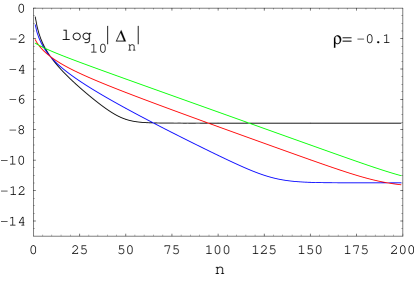
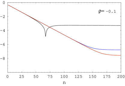
Figure 1. Left: Plot of $\log_{10}|\Delta_{n}|$ vs $n$ for the iteration of equation (156) with parameters $\rho=-0.1$ and $\beta=1$ (black), 0.5 (blue), 0.1 (red), 0.01 (green), and initial condition $F_{0}$ given by the inverse Gamma distribution. Right: plot of $\log_{10}|\mu_{1}(n)-\frac{e^{\rho}}{1-e^{\rho}}|$ vs $n$, with $\mu_{1}(n)$ the estimate of the first moment of $X_{\infty}$ after $n$ iterations. Same parameters as for the left plot.

These plots show also the impact of the $\rho$ parameter on the shape of the density function $F(u;\beta,\rho)$. As expected, negative values of $\rho$ increase the density at small values of $X_{\infty}$, while positive values depress it, and increase the contribution of the right tail.

As a test for the quality of the numerical solution we computed the first moment $\mathbb{E}[X_{\infty}]$ using the density function $f(x;\beta,\rho)$. As discussed in Section 5, this moment is finite for $\rho<0$ and is given by $\mu_{1}=\mathbb{E}[X_{\infty}]=\frac{e^{\rho}}{1-e^{\rho}}$. For $\rho=-0.1$, the convergence of the first moment to the theoretical value is shown in Figure 1 (right) which shows plots of $\log_{10}|\mu_{1}(n)-\frac{e^{\rho}}{1-e^{\rho}}|$ vs $n$ for several values of $\beta$, with $\mu_{1}(n)=\int_{0}^{\infty}xf_{n}(x;\beta,\rho)dx$. The spike in the $\beta=1$ plot is due to a change of sign of the difference $\mu_{1}(n)-\frac{e^{\rho}}{1-e^{\rho}}$.

The numerical values of the $(\beta,\rho)$ parameters used for these simulations cover the range of realistic values corresponding to practical applications. Typical values used in simulations for the equities model are $\mu=0.06,\sigma=0.2$ [15]. Assuming $r=0.01-0.05$ for the deterministic discount rate, gives that $m=-\mu-r$ takes values between -0.07 and -0.11.

Assuming a annuity with monthly payments $\tau=1/12$ the parameters determining the shape of the annuity density distribution are $\beta=0.0033,-\rho=0.006-0.009$. For a yearly annuity $\tau=1$ the parameters are $\beta=0.04,-\rho=0.07-0.11$. As seen from Figure 1 the convergence properties of the iterative procedure for solving the equation (156) for these parameter values are good, and the iteration converges with a moderate number of iterations of the order $n\sim 100$.

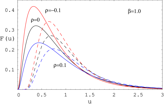
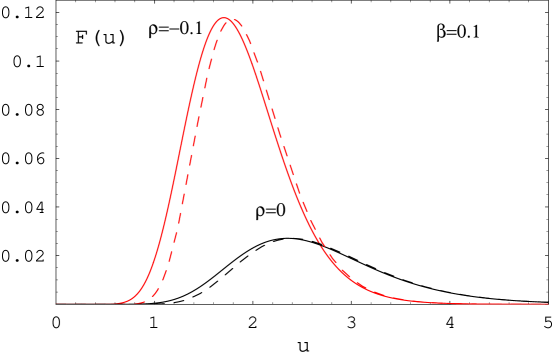
Figure 2. Plots of $F(u;\beta,\rho)$ (solid curves), the density function of $X_{\infty}$, for several values of $(\beta,\rho)$. The dashed curves show the continuous time approximation given by Proposition 15. Above: $\beta=1$, $\rho=-0.1$ (red), $\rho=0$ (black) and $\rho=0.1$ (blue). Below: $\beta=0.1$, $\rho=-0.1$ (red), $\rho=0$ (black).

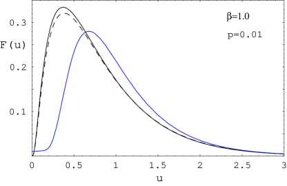
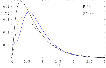
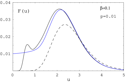
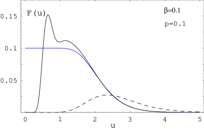
Figure 3. Plots of $F(u;\beta,\rho,p)$ (black curves), the density of $X_{N}$, for several choices of the parameters. Above: $\beta=1,\rho=0$, below: $\beta=0.1,\rho=0$. Left: $p=0.01$, right: $p=0.1$. The dashed curves correspond to $p=0$, and the blue curves show the continuous time approximation given by (102).

7.2. Annuities with Geometric Mortality

We consider here the distributional properties of the annuity with geometric mortality. Under the geometric mortality model, the density function $f(x;\beta,\rho,p)$ of the annuity $X_{N}$ is found by solving the integral equation in Proposition 16. After the change of variable $u=\log(x+1)$ this gives an integral equation for the function $F(u;\beta,\rho,p)=f(e^{u}-1;\beta,\rho,p)$.

(162) $$F(u;\beta,\rho,p) =p\frac{1}{\sqrt{2\pi\beta}(e^{u}-1)}e^{-\frac{1}{2\beta}(\log(e^{u}-1)+\frac{1}{2}\beta-\rho)^{2}}$$

$$\qquad\qquad+(1-p)e^{\beta-\rho}\int_{0}^{\infty}\frac{dw}{\sqrt{2\pi\beta}}e^{-\frac{1}{2\beta}(w-w_{0}(u))^{2}}F(w;\beta,\rho,p),$$

with $w_{0}(u)=\log(e^{u}-1)+\frac{3}{2}\beta-\rho$. We solve this integral equation by iteration, as in the case of the perpetuity $X_{\infty}$.

What is a reasonable range for the parameter $p$ of the geometric mortality model? We will constrain this parameter by matching to the Makeham model, which is one of the popular models for mortality rates [6]. Under this model the yearly mortality rate $\mu(a)$ is specified by the functional form [15]

(163) $$\mu(a)=A+Be^{\beta x}.$$

The model parameters are [6]

(164) $$A=0.0007\,,\qquad B=5\cdot 10^{-5}\,,\qquad\beta=0.0921\,.$$

We will match the geometric mortality model parameter $p$ to this realistic model. We consider two possible approaches.

i) Matching the expected life average, conditional on survival at age $a_{0}$. This gives the equation

(165) $$\mathbb{E}[a|a_{0}]=\int_{a_{0}}^{\infty}tp_{s}(t)\mu(t)dt=a_{0}+\frac{1}{p},$$

where the conditional survival probability $p_{s}(a|a_{0})$ is given by

(166) $$p_{s}(a|a_{0})=\exp\left(-\int_{a_{0}}^{a}ds\mu(s)\right).$$

This method gives $p=0.06443$ for $a_{0}=65$.

ii) Matching the mortality rates at age $a_{0}$. This gives the relation

(167) $$\mu(a_{0})=p(1-p)^{a_{0}}.$$

This method gives $p=0.02132$ for $a_{0}=65$.

The two values of $p$ determined as above span a range of realistic values, with i) being on the upper side of the realistic estimates for the $p$ parameter, while ii) is on the lower side of the range. A more precise matching is possible, using the result noted in [21] that any positive-definite discrete distribution can be approximated arbitrarily close by an appropriate linear combination of geometric distributions. A similar result holds in continuos time [14], and states that any positive definite continuous distribution can be approximated arbitrarily close by an appropriate linear combination of exponential distributions.

In order to study the effect of the geometric mortality on the shape of the density of $X_{N}$, we show in Figure 3 the results with $p=0.01$ and $p=0.1$ (black curves), comparing with the results for the density of $X_{\infty}$ ($p=0$) (dashed curves). The remaining parameters are $\beta=1$ (above) and $\beta=0.1$ (lower) and $\rho=0$. As expected, the effect of turning on a non-zero mortality rate $p$ is to increase the density at low values of $X_{N}$ and decrease the contribution of larger values of $X_{N}$.

In the small $\tau$ limit the distribution of $\tau X_{N}$ is expected to approach the distribution of the time integral of the GBM up to an exponentially distributed time $Y_{T_{\lambda}}$, as stated in (102). The asymptotic continuous time distribution is shown as the blue curves in Figure 3. The agreement with the continuous time result is seen to become better for smaller values of $\beta,p$, as predicted by equation (102). The plots in Figure 3 show that the approach to the continuous time limit is qualitatively different in the right and left tails of the distribution. While the right tail has a similar shape to that of the continuous time distribution (shown as the blue curve), the left tail displays very different qualitative behavior in the continuous and discrete time. We note two main differences in the left tail behavior:

i) the discrete time density of $X_{N}$ vanishes as $X_{N}\to 0$, while the continuous time density of $Y_{T_{\lambda}}$ approaches a finite value at origin $\phi_{\lambda}(0;\beta,\rho,p)=p$, as shown in Proposition 30.

ii) for certain parameter values, the discrete time density of $X_{N}$ has a bimodal distribution, with a peak visible near small values of $X_{N}$. This is due to the contribution to the density from events with killing at the first time of the annuity. In contrast, the density of the asymptotic continuous time distribution of $Y_{T_{\lambda}}$ has a unimodal shape.

The average value of the annuity is known exactly from Section 5

(168) $$\mathbb{E}[X_{N}]=\frac{e^{\rho}}{1-(1-p)e^{\rho}}\,.$$

We checked the quality of the numerical solution by computing this expectation by numerical quadrature and confirming good agreement with the theoretical result. For $p=0.1,\rho=0$ with $n=200$ iterations we get $\mathbb{E}[X_{N}]=9.9998$ which is close to the theoretical result ($\mathbb{E}[X_{N}]=10$).

Following [15] we compute the shortfall probability

(169) $$\mathbb{P}_{qK}=\mathbb{P}(X_{N}>(1+q)K)\,,$$

with $K=\mathbb{E}[X_{N}]$ and $q=0,0.5$. This measures the probability that an initial investment in the amount of 100% and 150% of the average annuity value, respectively, will not be sufficient to make the required payments on the annuity. The results are given in Table 1, for the same parameters $(\beta,p)$ as in Figure 3. In the last column we show the continuous time result for the shortfall probability given by

(170) $$\mathbb{P}_{qK}^{\tau=0}=\bar{\Phi}_{\lambda}\left(\frac{1}{2}\sigma^{2}K(1+q);\alpha,\beta\right),$$

with $\bar{\Phi}_{\lambda}$ given in (180). The difference with the discrete time result shows the effect of the discrete time nature of the annuity $X_{N}$ on its distribution and tail behavior. We note that, for the parameters considered, the discrete time and continuous time shortfall probabilities are very similar, the difference between them being below 1%. The agreement improves for smaller $\beta,p$, as expected from the asymptotic result of Proposition 20. We conclude that the continuous time approximation is reasonably good for practical purposes in the right tail of the annuity distribution, although the left tail can have very different behavior even for comparatively small values of $\beta,p$.

Table 1. Shortfall probabilities $\mathbb{P}_{qK}$ for a single-life annuity with discrete time payouts, for several choices of the model parameters. The last column shows the continuous time result given by equation (170).

$\beta$	$\rho$	$p$	$\mathbb{E}[X_{N}]$	$q$	$(1+q)K$	$\mathbb{P}_{qK}$	$\mathbb{P}_{qK}^{\tau=0}$
1	0	0.1	10	0	10	0.10852	0.10658
1	0	0.1	10	0.5	15	0.07122	0.06849
1	0	0.01	100	0	100	0.01781	0.01783
1	0	0.01	100	0.5	150	0.01187	0.01183
0.1	0	0.1	10	0	10	0.26821	0.27067
0.1	0	0.1	10	0.5	15	0.15846	0.15899
0.1	0	0.01	100	0	100	0.10625	0.10658
0.1	0	0.01	100	0.5	150	0.06853	0.06849
1.0	-0.1	0.1	4.87398	0	4.87398	0.16415	0.17072
1.0	-0.1	0.1	4.87398	0.5	7.31098	0.10509	0.10605
1.0	-0.1	0.01	8.68275	0	8.68275	0.12334	0.13083
1.0	-0.1	0.01	8.68275	0.5	13.02412	0.08018	0.08321
0.1	-0.1	0.1	4.87398	0	4.87398	0.34969	0.37558
0.1	-0.1	0.1	4.87398	0.5	7.31098	0.17592	0.19044
0.1	-0.1	0.01	8.68275	0	8.68275	0.32828	0.35577
0.1	-0.1	0.01	8.68275	0.5	13.02412	0.15949	0.17039

7.3. Application to Pricing Asian Options

We illustrate in this section the application of the methods discussed in Section 6 for pricing Asian options in the Black-Scholes model with discrete time averaging. We also discuss the conditions of applicability of the methods of approximating the distribution of the finite sum of GBM with the infinite sum $X_{\infty}$ or integral $Y_{\infty}$, as proposed in [31].

Theorem 22 gives a method for computing recursively the probability density function of $X_{n}$, the finite sum of GBM. This can be used to price Asian options with discrete time sampling in the BS model. For a more efficient calculation of the integral we change variables as in (156).

Using this method we priced Asian options with discrete sampling under the scenarios considered in Vecer’s paper [37]: $\sigma=0.4,r=0.1,T=1,K=100$, spot price $S_{0}=95,100,105$ and several choices for the number of time steps $n=T/\tau$ from 10 to 1000. Table 2 shows the results of the calculation for the discounted call Asian option price $C(K,T)=e^{-rT}\mathbb{E}[(X_{n}/n-K)_{+}]$. The results are in good agreement with those obtained by Vecer (Table B in [37]) using a PDE method proposed in [36], by Curran [8] using a method based on conditioning on the geometric average, and by Tavella-Randall [34] using the PDE method of Rogers and Shi [32].

The quality of the numerical integration was checked by computing also the expectation $\mathbb{E}[X_{n}]$ and checking that it agrees with the exact theoretical result, given by

(171) $$\mathbb{E}[X_{n}]=S_{0}\sum_{k=1}^{n}e^{kr\tau}=S_{0}\frac{e^{nr\tau}-1}{1-e^{-r\tau}},$$

up to four significant decimal points. We also priced put options and checked that put-call parity is satisfied to four significant decimal points.

(172) $$C(K,T)-P(K,T)=e^{-rT}\left(\frac{S_{0}}{rT}(e^{rT}-1)-K\right)\,.$$

Table 2. Numerical results for Asian options with discrete sampling in the Black-Scholes model using the method described in this paper, under the scenarios discussed in text. The results are compared with those of Vecer [37], Curran [8] and Tavella-Randall [34].

$n$	$S_{0}$	$C(K,T)$	Vecer	Curran	Tavella-Randall
10	95	9.2239	9.2228	9.2197	9.2149
10	100	12.0424	12.042	12.0390	12.0348
10	105	15.2243	15.2234	15.2202	15.2168
25	95	8.7086	8.708	8.7053	8.6974
25	100	11.4910	11.4906	11.4881	11.4803
25	105	14.6510	14.651	14.6483	14.6415
50	95	8.5371	8.5367	8.5340	8.5383
50	100	11.3070	11.3068	11.3043	11.2982
50	105	14.4611	14.4601	14.4575	14.4519
125	95	8.4347	8.4339	8.4314	8.4304
125	100	11.1974	11.1967	11.1940	11.1929
125	105	14.3459	14.3455	14.3430	14.3424
250	95	8.4006	8.4001	8.3972	8.3972
250	100	11.1607	11.1600	11.1572	11.1573
250	105	14.3081	14.3073	14.3048	14.3054
500	95	8.3831	8.3826	8.3801	8.3804
500	100	11.1422	11.1416	11.1388	11.1392
500	105	14.2887	14.2881	14.2857	14.2866
1000	95	8.3718	8.3741	8.3715	8.3719
1000	100	11.1301	11.1322	11.1296	11.1300
1000	105	14.2754	14.2786	14.2762	14.2771

Next we discuss the pricing of Asian options under the following approximations:

1. Approximating the distribution of $\tau X_{n}$ with that of $Y_{\infty}$, the infinite time integral of the GBM. This is the theoretical basis of the approximation of Milevsky and Posner [31], who propose a moment matching approach for modeling the distribution of $X_{n}$ with an inverse Gamma distribution.

2. Approximating the distribution of $X_{n}$ with that of $X_{\infty}$, the infinite sum of GBM sampled on discrete times.

These approximations are expected to be most precise in the limit of a very large number of sampling times $n\to\infty$. We note that these approximations can only be used if $r<0$, which is the condition for the existence of the limiting distributions for $Y_{\infty}$ (Theorem 1) and for $X_{\infty}$ (Proposition 4), and for the finiteness of the expectations $\mathbb{E}[Y_{\infty}]<\infty,\mathbb{E}[X_{\infty}]<\infty$.

Allowing also for a continuously paid dividend yield $q$ this condition reads $r-q<0$. In usual applications to equity options the difference $r-q$ is positive, although it could become negative in low rates environments. A natural case where negative drifts appear is for Asian options on FX rates. Denote $X_{t}$ a currency exchange rate, defined as the number of units of domestic currency corresponding to one unit of foreign currency. One of the simplest models for the dynamics of exchange rates is to assume that $X_{t}$ satisfies the diffusion $dX_{t}/X_{t}=(r_{d}-r_{f})dt+\sigma_{X}dW_{t}$ in the domestic currency risk-neutral measure. The drift of $X_{t}$ is given by the difference between the domestic and foreign interest rates, such that the condition of applicability of the approximations mentioned above is $r_{d}-r_{f}<0$.

Another condition for the applicability of the approximations (1),(2) is that the expectations of $\tau X_{n}$ and $Y_{\infty}$ ($X_{n}$ and $X_{\infty}$) should be sufficiently close. For (1) this condition reads $\tau\frac{e^{nr\tau}-1}{1-e^{-r\tau}}\sim-\frac{1}{r}$ which requires in addition $n\tau\gg 1$ and $|r\tau|\ll 1$. In practice this requires that the option maturity $T$ be sufficiently long such that $|rT|\gg 1$, and that the time step is sufficiently small. On the other hand, the corresponding condition for the approximation (2) is $\frac{e^{nr\tau}-1}{1-e^{-r\tau}}\sim\frac{1}{e^{-r\tau}-1}$ which requires only $n\gg 1$ and $n\tau\gg 1$ but does not impose any constraints on the size of the time step $\tau$.

Appendix A The Law of the Time Integral of the GBM Up to an Exponentially Distributed Time

We summarize in this Appendix for the convenience of the reader a few known results concerning the distribution of the time integral of GBM up to an exponentially distributed random time. These results have been derived in [39]. See also [13] for a survey of related results.

Let us define

(173) $$Y_{T_{\lambda}}:=\int_{0}^{T_{\lambda}}dte^{\sigma W_{t}+(m-\frac{1}{2}\sigma^{2})t}.$$

the time integral of the GBM up to an exponentially distributed time $T_{\lambda}\sim\mathbf{Exp}(\lambda)$. The probability density function of $Y_{T_{\lambda}}$ is given by the following result.

Proposition 28.

The probability density function of $Y_{T_{\lambda}}$ is given by

(174) $$\phi_{\lambda}(z;\sigma,m,\lambda)=\frac{1}{2}\sigma^{2}\varphi\left(\frac{1}{2}\sigma^{2}z;\alpha,\beta\right),$$

where

(175) $$\varphi(y;\alpha,\beta)=\frac{\alpha\beta\Gamma(\alpha)}{\Gamma(\alpha+\beta+1)}y^{-\beta-1}{}_{1}F_{1}\left(\beta+1,\alpha+\beta+1;-\frac{1}{y}\right),$$

which is the density of the random variable $Y:=B_{1,\alpha}/G_{\beta}$ with $B_{1,\alpha}$ and $G_{\beta}$ being independent random variables distributed as Beta and Gamma distributions. Their densities are

(176) $$\varphi_{B}(b) = \alpha(1-b)^{\alpha-1}\,,\quad b\in[0,1],$$

(177) $$\varphi_{G}(g) = \frac{1}{\Gamma(\beta)}g^{\beta-1}e^{-g}\,,\quad g\in[0,\infty)\,.$$

The constants $\alpha,\beta$ are

(178) $$\alpha = \frac{1}{2\sigma^{2}}\left(2m-\sigma^{2}+\sqrt{(2m-\sigma^{2})^{2}+8\lambda\sigma^{2}}\right),$$

(179) $$\beta = \frac{1}{2\sigma^{2}}\left(-2m+\sigma^{2}+\sqrt{(2m-\sigma^{2})^{2}+8\lambda\sigma^{2}}\right).$$

The result (175) agrees with the explicit result for this density in [13] (fourth equation from bottom on p. 12).

We note that for $\lambda>0$, the constant $\alpha$ is always strictly positive. This is a necessary condition for $B_{1,\alpha}$ to exist.

Proposition 29 (Right tail behavior).

The right tail of the distribution $Y_{T_{\lambda}}$ is given by:

(180) $$\mathbb{P}(Y_{T_{\lambda}}>z)=\int_{z}^{\infty}dx\phi_{\lambda}(x;\sigma,m,\lambda)=\int_{\frac{1}{2}\sigma^{2}z}^{\infty}dy\varphi(y;\alpha,\beta)=\bar{\Phi}_{\lambda}\left(\frac{1}{2}\sigma^{2}z;\alpha,\beta\right),$$

where $\bar{\Phi}_{\lambda}(y;\alpha,\beta)$ is the complementary cumulative distribution of $Y:=B_{1,\alpha}/G_{\beta}$ with $B_{1,\alpha}$ and $G_{\beta}$ being independent random variables distributed as Beta and Gamma distributions, which has the right tail asymptotics as $y\rightarrow\infty$:

(181) $$\bar{\Phi}_{\lambda}(y;\alpha,\beta)=\int_{y}^{\infty}dw\varphi(w;\alpha,\beta)=\frac{\alpha\Gamma(\alpha)}{\Gamma(\alpha+\beta+1)}y^{-\beta}(1+O(y^{-1})).$$

We note that the exponent is the same as for the right tail asymptotics of the discrete time sum of GBM with geometric mortality derived in (73). This can be seen by replacing $p=\lambda\tau$ in (73) and approximating $\log(1-p)\sim-p$. This gives for the exponent

(182) $$\mu=\frac{1}{2\sigma^{2}}(-2m+\sigma^{2}+\sqrt{(2m-\sigma^{2})^{2}+8\sigma^{2}\lambda}),$$

which agrees precisely with $\beta$ defined in (179).

Proposition 30 (Left tail behavior).

The left tail behavior of the density $\varphi(y;\alpha,\beta)$ is

(183) $$\lim_{y\to 0}\varphi(y;\alpha,\beta)=\alpha\beta=\frac{2}{\sigma^{2}}\lambda\,.$$

The probability density $\varphi(y;\alpha,\beta)$ approaches a non-vanishing constant near the origin $y\to 0$.

This tail behavior is different from the discrete time case, where we find that the density of $X_{N}$ always vanishes near the zero point. This behavior implies that all negative moments $\mathbb{E}[Y_{T_{\lambda}}^{\theta}]$ with $\theta\leq-1$ do not exist. On the other hand, for the discrete time case all the negative moments of $X_{N}$ are finite.

Limiting case $\lambda=0$. This corresponds to $T_{\lambda}\to\infty$, since the expectation of $T_{\lambda}$ under the exponential distribution is

(184) $$\mathbb{E}[T_{\lambda}]=\frac{1}{\lambda}.$$

We distinguish two cases:

i) $m<\frac{1}{2}\sigma^{2}$. We have $(\alpha,\beta)=(0,1-\frac{2m}{\sigma^{2}})$;

ii) $m>\frac{1}{2}\sigma^{2}$. This gives a negative $\alpha$, which is meaningless since the $\mbox{Beta}(1,\alpha)$ distribution is defined only for $\alpha\geq 0$.

The confluent hypergeometric function in case (i) can be expressed in closed form using the identity ${}_{1}F_{1}(b,b,z)=e^{z}$, which holds for any positive integer $b$. We have

(185) $$\varphi\left(y;0,1-\frac{2m}{\sigma^{2}}\right)=\frac{1}{\Gamma(1+\frac{2m}{\sigma^{2}})}y^{-2+\frac{2m}{\sigma^{2}}}e^{-1/y}.$$

Using (174) we get the density function of the infinite time integral of the GBM

$$\lim_{\lambda\to 0}\phi_{\lambda}(z;\sigma,m,0) = \frac{1}{2}\sigma^{2}\frac{1}{\Gamma(1+\frac{2m}{\sigma^{2}})}\left(\frac{1}{2}\sigma^{2}z\right)^{-2+\frac{2m}{\sigma^{2}}}\exp\left(-\frac{2}{\sigma^{2}z}\right)$$

$$= (2/\sigma^{2})^{1-\frac{2m}{\sigma^{2}}}\frac{1}{(z^{2})^{1-\frac{m}{\sigma^{2}}}}\frac{1}{\Gamma(1+\frac{2m}{\sigma^{2}})}\exp\left(-\frac{2}{\sigma^{2}z}\right).$$

This agrees with $\phi_{\infty}(z;\sigma,m)$ in equation (9).

Proof of Proposition 28.

Step 1. Use a time change to relate $Y_{T_{\lambda}}$ to a certain integral for which we know the distribution from Yor’s paper [39]. This is

(187) $$Y_{t_{\lambda}}^{(\mu)}=\int_{0}^{t_{\lambda}}e^{2\mu s+2W_{s}}ds,$$

where $t_{\lambda}\sim\mathbf{Exp}(\lambda)$. It is known [39] that the distribution of this integral is

(188) $$2Y_{t_{\lambda}}^{(\mu)}=\frac{B_{1,\hat{\alpha}}}{G_{\hat{\beta}}},$$

with $\hat{\alpha}=\frac{1}{2}\mu+\frac{1}{2}\sqrt{\mu^{2}+2\lambda}$ and $\hat{\beta}=-\frac{1}{2}\mu+\frac{1}{2}\sqrt{\mu^{2}+2\lambda}$.

It is easy to see, using a time change, that we have

(189) $$Y_{T_{\lambda}}=\frac{4}{\sigma^{2}}Y_{\frac{1}{4}\sigma^{2}T_{\lambda}}^{(\frac{2m}{\sigma^{2}}-1)}.$$

We have $\frac{1}{4}\sigma^{2}T_{\lambda}\sim\mathbf{Exp}(\frac{4}{\sigma^{2}}\lambda)$. Substituting $\lambda\to\frac{4}{\sigma^{2}}\lambda$ and $\mu\to\frac{2m}{\sigma^{2}}-1$ into the expressions for $\hat{\alpha},\hat{\beta}$ we get the results (178) and (179) for the parameters $\alpha,\beta$.

Step 2. Use the result [39]

(190) $$Y_{T_{\lambda}}=\frac{2}{\sigma^{2}}\frac{B_{1,\alpha}}{G_{\beta}}$$

in distribution. Denoting $y=b/g$ the ratio of the two independent random variables, it is easy to show by explicit calculation that its pdf is given by (175). Taking into account also the factor $2/\sigma^{2}$ we get the final result (174). ∎

Proof of Proposition 30.

We prove here the left tail asymptotics. This follows from the asymptotic expansion for the confluent hypergeometric function of large negative argument:

(191) $${}_{1}F_{1}\left(\beta+1,\alpha+\beta+1,-\frac{1}{y}\right)\sim\frac{\Gamma(\alpha+\beta+1)}{\Gamma(\alpha)}y^{\beta+1}\,,\quad\text{as $y\to 0$}.$$

This is obtained from the asymptotics for large positive argument

(192) $${}_{1}F_{1}(a,b,z)\sim\frac{\Gamma(b)}{\Gamma(a)}e^{z}z^{a-b}\,,\qquad\text{as $z\to\infty$},$$

together with the Kummer transformation relation

(193) $${}_{1}F_{1}(a,b,z)=e^{z}{}_{1}F_{1}(b-a,b,-z)\,.$$

∎

Appendix B Proofs

Proof of Theorem 13.

(i) We have

(194) $$\left|\tau\sum_{i=1}^{N}e^{\sigma W_{t_{i-1}}+(m-\frac{1}{2}\sigma^{2})t_{i-1}}-\int_{0}^{T}e^{\sigma W_{t}+(m-\frac{1}{2}\sigma^{2})t}dt\right|$$

$$\leq\sum_{i=1}^{N}\left|\tau e^{\sigma W_{t_{i-1}}+(m-\frac{1}{2}\sigma^{2})t_{i-1}}-\int_{t_{i-1}}^{t_{i}}e^{\sigma W_{t}+(m-\frac{1}{2}\sigma^{2})t}dt\right|$$

$$\leq\tau\sum_{i=1}^{N}\max_{t_{i-1}\leq t\leq t_{i}}\left|e^{\sigma W_{t}+(m-\frac{1}{2}\sigma^{2})t}-e^{\sigma W_{t_{i-1}}+(m-\frac{1}{2}\sigma^{2})t_{i-1}}\right|.$$

Add and subtract in each term $e^{\sigma W_{t}+(m-\frac{1}{2}\sigma^{2})t_{i-1}}$ and use the triangle inequality. Each term in the sum is bounded from above as

(195) $$\tau\max_{t_{i-1}\leq t\leq t_{i}}\left|e^{\sigma W_{t}+(m-\frac{1}{2}\sigma^{2})t}-e^{\sigma W_{t_{i-1}}+(m-\frac{1}{2}\sigma^{2})t_{i-1}}\right|\leq T_{1}^{(i)}+T_{2}^{(i)},$$

where we denoted

(196) $$T_{1}^{(i)} = \tau\max_{t_{i-1}\leq t\leq t_{i}}\left|e^{\sigma W_{t}}-e^{\sigma W_{t_{i-1}}}\right|e^{(m-\frac{1}{2}\sigma^{2})t_{i-1}},$$

(197) $$T_{2}^{(i)} = \tau\max_{t_{i-1}\leq t\leq t_{i}}e^{\sigma W_{t}}\left|e^{(m-\frac{1}{2}\sigma^{2})t}-e^{(m-\frac{1}{2}\sigma^{2})t_{i-1}}\right|.$$

We would like to show that the following sum converges to zero as $\tau\to 0$

(198) $$\lim_{\tau\to 0,\tau N=T}\sum_{i=1}^{N}\mathbb{E}\left[T_{1}^{(i)}+T_{2}^{(i)}\right]\to 0.$$

We bound each term in turn.

(199) $$\mathbb{E}\left[T_{1}^{(i)}\right] =\tau\mathbb{E}\left[e^{\sigma W_{t_{i-1}}+(m-\frac{1}{2}\sigma^{2})t_{i-1}}\max_{t_{i-1}\leq t\leq t_{i}}\left|e^{\sigma(W_{t}-W_{t_{i-1}})}-1\right|\right]$$

$$=\tau e^{mt_{i-1}}\mathbb{E}\left[\max_{t_{i-1}\leq t\leq t_{i}}\left|e^{\sigma(W_{t}-W_{t_{i-1}})}-1\right|\right]$$

$$\leq\tau e^{mt_{i-1}}\mathbb{E}\left[\max_{0\leq t\leq\tau}|e^{\sigma W_{t}}-1|\right]$$

$$\leq\tau e^{mt_{i-1}}\mathbb{E}\left[e^{\sigma\max_{0\leq t\leq\tau}W_{t}}-e^{\sigma\min_{0\leq t\leq\tau}W_{t}}\right]$$

$$=\tau e^{mt_{i-1}}\left(\mathbb{E}\left[e^{\sigma|W_{\tau}|}\right]-\mathbb{E}\left[e^{-\sigma|W_{\tau}|}\right]\right),$$

where we used the reflection principle for Brownian motions. Summing over $i$ we have

(200) $$\sum_{i=1}^{N}\mathbb{E}\left[T_{1}^{(i)}\right] \leq\tau\frac{e^{m\tau N}-1}{e^{m\tau}-1}\left(\mathbb{E}\left[e^{\sigma|W_{\tau}|}\right]-\mathbb{E}\left[e^{-\sigma|W_{\tau}|}\right]\right)$$

$$=\tau\frac{e^{mT}-1}{e^{m\tau}-1}e^{\frac{1}{2}\sigma^{2}\tau}\cdot 2\left[\Phi(\sigma\sqrt{\tau})-\Phi(-\sigma\sqrt{\tau})\right]\rightarrow 0,$$

as $\tau\to 0$, where $\Phi(x):=\int_{-\infty}^{x}\frac{1}{\sqrt{2\pi}}e^{-y^{2}/2}dy$ is the cumulative distribution function of a standard normal random variable.

The second term is bounded in a similar way.

(201) $$\mathbb{E}\left[T_{2}^{(i)}\right] \leq\tau\mathbb{E}\left[\max_{t_{i-1}<t<t_{i}}e^{\sigma(W_{t}-W_{t_{i-1}})}e^{\sigma W_{t_{i-1}}+(m-\frac{1}{2}\sigma^{2})t_{i-1}}\right]$$

$$\qquad\qquad\cdot\max_{t_{i-1}<t<t_{i}}\left|e^{(m-\frac{1}{2}\sigma^{2})(t-t_{i-1})}-1\right|\,.$$

The two factors in the expectation are again independent, so the expectation factors into their expectations. The supremum over the last factor depends on the sign of $m-\frac{1}{2}\sigma^{2}$. For $m-\frac{1}{2}\sigma^{2}>0$ this is $e^{(m-\frac{1}{2}\sigma^{2})\tau}-1$ and for $m-\frac{1}{2}\sigma^{2}<0$ this is $1-e^{(m-\frac{1}{2}\sigma^{2})\tau}$. This gives

(202) $$\mathbb{E}\left[T_{2}^{(i)}\right] \leq\tau\mathbb{E}\left[\max_{t_{i-1}<t<t_{i}}e^{\sigma(W_{t}-W_{t_{i-1}})}\right]e^{mt_{i-1}}\mbox{sgn}(m-\frac{1}{2}\sigma^{2})\left(e^{(m-\frac{1}{2}\sigma^{2})\tau}-1\right)$$

$$\leq 2\Phi(\sigma\sqrt{\tau})\tau e^{\frac{1}{2}\sigma^{2}\tau}e^{mt_{i-1}}\mbox{sgn}(m-\frac{1}{2}\sigma^{2})\left(e^{(m-\frac{1}{2}\sigma^{2})\tau}-1\right).$$

$$=2\Phi(\sigma\sqrt{\tau})\tau e^{mt_{i-1}}\left|e^{m\tau}-e^{\frac{1}{2}\sigma^{2}\tau}\right|.$$

This is summed over $i=1,N$ as previously, and the result is finite and goes to zero as $\tau\to 0$.

(ii) The case of the infinite maturity $T\to\infty$ is treated analogously, except that one requires $m<0$ in order to ensure the convergence of the sums $\sum_{i=1}^{\infty}T_{1}^{(i)}$ and $\sum_{i=1}^{\infty}T_{2}^{(i)}$. ∎

Proof of Theorem 19.

Step 1. We start by proving the limit

(203) $$\lim_{\tau\to 0}\left|\tau\sum_{i=1}^{N}e^{\sigma W_{t_{i-1}}+(m-\frac{1}{2}\sigma^{2})t_{i-1}}-\int_{0}^{N\tau}e^{\sigma W_{t}+(m-\frac{1}{2}\sigma^{2})t}dt\right|=0$$

in probability as $\tau\rightarrow 0$. Here $N$ is a geometrically distributed random variable with parameter $p$.

Consider the expectation

(204) $$\Delta_{\tau}:=\mathbb{E}\left[\left|\tau\sum_{i=1}^{N}e^{\sigma W_{t_{i-1}}+(m-\frac{1}{2}\sigma^{2})t_{i-1}}-\int_{0}^{N\tau}e^{\sigma W_{t}+(m-\frac{1}{2}\sigma^{2})t}dt\right|\right]\,.$$

In order to prove (203) it is sufficient to show $\lim_{\tau\to 0}\Delta_{\tau}=0$.

This expectation is written as

(205) $$\Delta_{\tau}=\sum_{k=1}^{\infty}p(1-p)^{k-1}\mathbb{E}\left[\left|\tau\sum_{i=1}^{k}e^{\sigma W_{t_{i-1}}+(m-\frac{1}{2}\sigma^{2})t_{i-1}}-\int_{0}^{k\tau}e^{\sigma W_{t}+(m-\frac{1}{2}\sigma^{2})t}dt\right|\right]\,.$$

The expectations with fixed $k\in\mathbb{N}$ are bounded from above as shown in the proof of Theorem 13. We have

(206) $$\mathbb{E}\left[\left|\tau\sum_{i=1}^{k}e^{\sigma W_{t_{i-1}}+(m-\frac{1}{2}\sigma^{2})t_{i-1}}-\int_{0}^{k\tau}e^{\sigma W_{t}+(m-\frac{1}{2}\sigma^{2})t}dt\right|\right]\leq\sum_{i=1}^{k}\mathbb{E}[T_{1}^{(i)}+T_{2}^{(i)}]$$

$$\leq(e^{mk\tau}-1)R_{\tau}$$

where we have from equation (200)

(207) $$\sum_{i=1}^{k}\mathbb{E}[T_{1}^{(i)}]\leq\tau\frac{e^{mk\tau}-1}{e^{m\tau}-1}e^{\frac{1}{2}\sigma^{2}\tau}2[\Phi(\sigma\sqrt{\tau})-\Phi(-\sigma\sqrt{\tau})]$$

and from equation (202)

(208) $$\sum_{i=1}^{k}\mathbb{E}[T_{2}^{(i)}]\leq\tau\frac{e^{mk\tau}-1}{e^{m\tau}-1}\left|e^{m\tau}-e^{\frac{1}{2}\sigma^{2}\tau}\right|2\Phi(\sigma\sqrt{\tau})$$

We combined these two inequalities in the last line of (206) by introducing

$$R_{\tau} := \tau\frac{1}{e^{m\tau}-1}e^{\frac{1}{2}\sigma^{2}\tau}2[\Phi(\sigma\sqrt{\tau})-\Phi(-\sigma\sqrt{\tau})]$$

$$+ \tau\frac{1}{e^{m\tau}-1}\left|e^{m\tau}-e^{\frac{1}{2}\sigma^{2}\tau}\right|2\Phi(\sigma\sqrt{\tau})\,.$$

Substituting (206) into (205) we have

(210) $$\Delta_{\tau}\leq R_{\tau}\sum_{k=1}^{\infty}p(1-p)^{k-1}(e^{km\tau}-1)=\left(\frac{pe^{m\tau}}{1-e^{m\tau}(1-p)}-1\right)R_{\tau}\,.$$

The sum over $k$ converges provided that $(1-p)e^{m\tau}<1$. A sufficient condition for this to hold for any $\tau>0$ is $m<\lambda$.

As $\tau\to 0$, we have

(211) $$\lim_{\tau\to 0}\left(\frac{pe^{m\tau}}{1-e^{m\tau}(1-p)}-1\right)=\frac{m}{\lambda-m}$$

and

(212) $$\lim_{\tau\to 0}R_{\tau}=0$$

Combining these results gives $\lim_{\tau\to 0}\Delta_{\tau}=0$ which completes the proof of the result stated.

Step 2. In the next step we prove

(213) $$\int_{0}^{N\tau}e^{\sigma W_{t}+(m-\frac{1}{2}\sigma^{2})t}dt\rightarrow\int_{0}^{T_{\lambda}}e^{\sigma W_{t}+(m-\frac{1}{2}\sigma^{2})t}dt,$$

in distribution as $\tau\rightarrow 0$. For any $x>0$,

(214) $$\mathbb{P}\left(\int_{0}^{N\tau}e^{\sigma W_{t}+(m-\frac{1}{2}\sigma^{2})t}dt\leq x\right)$$

$$=\sum_{k=1}^{\infty}\mathbb{P}\left(\int_{0}^{k\tau}e^{\sigma W_{t}+(m-\frac{1}{2}\sigma^{2})t}dt\leq x\right)(1-\lambda\tau)^{k-1}\lambda\tau,$$

$$=\frac{1}{1-\lambda\tau}\sum_{k=1}^{\infty}\mathbb{P}\left(\int_{0}^{k\tau}e^{\sigma W_{t}+(m-\frac{1}{2}\sigma^{2})t}dt\leq x\right)\left((1-\lambda\tau)^{\frac{1}{\tau}}\right)^{k\tau}\lambda\tau$$

$$\rightarrow\int_{0}^{\infty}\mathbb{P}\left(\int_{0}^{u}e^{\sigma W_{t}+(m-\frac{1}{2}\sigma^{2})t}dt\leq x\right)\lambda e^{-\lambda u}du$$

$$=\mathbb{P}\left(\int_{0}^{T_{\lambda}}e^{\sigma W_{t}+(m-\frac{1}{2}\sigma^{2})t}dt\leq x\right),$$

as $\tau\rightarrow 0$. Hence, we proved the desired result. ∎

References

• [1] Alsmeyer, G., A. Iksanov and U. Rösler (2009). On distributional properties of perpetuities. J. Theor. Probab. 22, 666-682.
• [2] American Academy of Actuaries (2005). Recommended approach for setting regulatory risk-based capital requirements for variable annuities and similar products. Boston, MA.
• [3] Asmussen, S., J. L. Jensen and L. Rojas-Nandayapa (2011). A Literature Review on Lognormal Sums, University of Queensland preprint.
• [4] Asmussen, S., L. Rojas-Nandayapa, Asymptotics of sums of lognormal random variables with Gaussian copula, Stat. Prob. Lett. 78, 2709-2714 (2008).
• [5] Bertoin, J. and M. Yor (2005). Exponential functionals of Lévy processes. Prob. Surveys 2, 191-212.
• [6] Bowers, N. L.  et al. (2007). Actuarial Mathematics (2nd Ed.) Society of Actuaries, Schaumburg, IL.
• [7] Carr, P., M. Schröder (2003). Bessel processes, the integral of geometric Brownian motion, and Asian options. Theory of Probability and its Applications 48, 400-425.
• [8] Curran, M. (1992), Beyond average intelligence, Risk, May 1992.
• [9] Davis, P. J. and P. Rabinowitz (2007). Methods of Numerical Integration (2nd Ed.) Dover Publications, New York, 2007
• [10] De Schepper A., M.Goovaerts, F. Delbaen (1992). The Laplace transform of certain annuities with exponential time distribution. Insurance: Mathematics and Economics 11 291-304.
• [11] Donati-Martin, C., Ghomrasni, R. and M. Yor. (2001). On certain Markov processes attached to exponential functionals of Brownian motion; application to Asian options. Rev. Math. Iberoam. 17, 179-193.
• [12] Dufresne, D. (1990). The distribution of a perpetuity, with applications to risk theory and pension funding. Scand. Actuar. J. 39-79.
• [13] Dufresne, D. (2005). Bessel processes and a functional of Brownian motion, in M. Michele and H. Ben-Ameur (Ed.), Numerical Methods in Finance, 35-57, Springer, 2005.
• [14] Dufresne, D. (2007a). Fitting combinations of exponentials to probability distributions, Applied Stochastic Models in Business and Industry 23, 23-48.
• [15] Dufresne, D. (2007b). Stochastic Life Annuities, North American Actuarial Journal 11(1), 136-157.
• [16] Dufresne, D. (2004). The lognormal approximation in financial and other computations. Adv. Appl. Prob. 36, 747-773.
• [17] Dufresne, D. (1996). On the stochastic equation $L(X)=L(B(X+C))$ and a property of the gamma distributions. Bernoulli 2, 287-291.
• [18] Feng, R.  and H. W. Volkmer (2012) Analytical calculation of risk measures for variable annuity guaranteed benefits. Insurance: Mathematics and Economics 51(4), 636-648.
• [19] Gao, X., H. Xu and D. Ye (2009). Asymptotic behavior of tail density for sum of correlated lognormal variables, Int. J. Math. and Math. Sciences, 2009, doi.10.1155/2009/630857.
• [20] Geman, H. and M. Yor, Bessel processes, Asian options and perpetuities, Math. Fin. 3, 349-375 (1993).
• [21] Gerber, H. U., E. S. W. Shiu and H. Yang, Geometric Stopping of a Random Walk and its Applications to Valuing Equity-linked Death Benefits, Insurance: Mathematics and Economics 64, 313-325 (2015).
• [22] Gjessing, H. K. and J. Paulsen, Present value distributions with applications to ruin theory and stochastic equations. Stoch. Proc. and their Applications 71, 123-144 (1997).
• [23] Goldie, C. M. (1991). Implicit renewal theory and tails of solutions of random equations. Ann. Appl. Probab. 1, 126-166.
• [24] Gulisashvili, A.  and P. Tankov (2016). Tail behavior of sums and differences of log-normal random variables. Bernoulli 22, No.1, 444-493.
• [25] Hardy, M. (2003) Investment Guarantees: Modeling and Risk Management for Equity-Linked Life Insurance. Wiley, New Jersey.
• [26] Kesten, H. (1973). Random difference equations and renewal theory for products of random matrices. Acta Mathematica. 131, 207-248.
• [27] Levy, E. (1992). Pricing European average rate currency options. Journal of International Money and Finance. 11, 474-491.
• [28] Mikosh, T., G. Samorodinsky and L. Takafori (2013). Fractional moments of solutions to stochastic recurrence equations. Journal of Applied Probability. 50, 969-982.
• [29] Pirjol, D. and L. Zhu (2015). Asymptotics for the discrete time average of the geometric Brownian motion and Asian options. Preprint.
• [30] Pirjol, D. and L. Zhu (2015). On the growth rate of a linear stochastic recursion with Markovian dependence. Journal of Statistical Physics. 160, 1354-1388.
• [31] Milevsky, M. and S. Posner. (1998). Asian Options, the Sum of Lognormals, and the Reciprocal Gamma Distribution, J. Fin. Quant. Analysis 33, 409.
• [32] Rogers, L., and Z. Shi (1995). The value of an Asian option, J. Appl. Prob. 32, 1077-1088.
• [33] Rolski, T., H. Schimidli, V. Schmidt and J. Teugels (1999). Stochastic Processes for Insurance and Finance. Wiley.
• [34] Tavella, D., and C. Randall (2000). Pricing financial instruments - the finite difference method. Wiley, 2000.
• [35] Vanduffel, S., Z. Shang, L. Henrard, J. Dhaene and E.A.Valdez (2008). Analytic bounds and approximations for annuities and Asian options. Insurance: Mathematics and Economics 42(3), 1109-1117.
• [36] Vecer, J. (2001), A new PDE approach for pricing arithmetic average Asian options, J. Comp. Finance 4(4), 105-113.
• [37] Vecer, J. (2002). Unified Asian pricing, Risk, June 2002, 113-115.
• [38] Vervaat, W. (1979). On a stochastic difference equation and a representation of non-negative infinitely divisible random variables. Adv. Appl. Prob. 11, 750-783.
• [39] Yor, M. (1992). Sur les lois des fonctionelles exponentielles du mouvement brownien, considerees en certains instants aleatoires. C. R. Acad. Sci. Paris Serie I 314, 951-956.
• [40] Yor, M. (1992). On some exponential functionals of Brownian motion. Adv. Appl. Prob. 24, 509-531.
• [41] Yor, M. (2001). Exponential functionals of Brownian motion and related processes. Springer Verlag, New York.
• [42] Zhu, L. (2015). Options with extreme strikes, Risks 3, 234-249.