Proving Linearizability via Branching Bisimulation

Abstract.

Linearizability and progress properties are key correctness notions for concurrent objects. However, model checking linearizability has suffered from the PSPACE-hardness of the trace inclusion problem. This paper proposes to exploit branching bisimulation, a fundamental semantic equivalence relation developed for process algebras which can be computed efficiently, in checking these properties. A quotient construction is provided which results in huge state space reductions. We confirm the advantages of the proposed approach on more than a dozen benchmark problems.

1. Introduction

A concurrent data structure, or a concurrent object, provides a set of methods that allow client threads to simultaneously access and manipulate a shared object. Linearizablity [17] is a widely accepted correctness criterion for implementations of concurrent objects. Intuitively, an implementation of a concurrent object is linearizable with respect to a sequential specification if every method call appears “to take effect”, i.e. changes the state of the object, instantaneously at some time point between its invocation and its response, behaving as defined by the specification. Such a time point, which corresponds to the execution of some program statement, is referred to as the linearization point of the method call. The difficulties (and confusions) encountered in verifying linearizability for concurrent data structures stemmed from the fact that the linearization points of different calls of the same method may correspond to different statements in the method’s, or even other method’s, program text.

The subtlety of linearization points can be illustrated using the heavily studied Herlihy and Wing queue algorithm [17], shown in Figure 1. It has two methods, Enq (enqueue) and Deq (dequeue). The queue is implemented by an array $AR$ of unbounded length, with $back$ as the index of the next unused slot in $AR$. Each element of $AR$ is initialized to a special value $null$, and $back$ is initialized to 1. An Enq execution contains two steps, it first gets a local copy $i$ of $back$ and increments $back$, then stores the new value at $AR[i]$. A Deq execution may take several steps to find a non-null element to be dequeued, by visiting $AR$ in ascending order, starting from index $1$ and ending at $back-1$. At each slot $i$, the current element $AR[i]$ is swapped with $null$. If Deq finds a non-$null$ value, it will return that value, otherwise it tries the next slot. If no element is found in the entire array, Deq restarts the search. The Enq and Deq methods can be executed concurrently by any number of client threads. Every execution step is atomic.

⬇

E0 Enq(x:T) {

E1 (i, back):=(back, back+1); /* increment */

E2 AR[i]:=x; /* store */

E3 return

E4 }

⬇

D0 Deq() {

D1 while true do {

D2 range := back;

D3 for (0 < i < range) do {

D4 (x, AR[i]):=(AR[i], null); /* swap */

D5 if (x != null) then return (x)

D6 } } }

Figure 1. Herlihy and Wing queue.

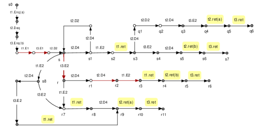
Figure 2. A part of the transition system for the Herlihy and Wing queue.

The behavior of a concurrent object system can be modeled as a labeled transition system. For the HW-queue example, consider a system of three client threads $t_{1}$, $t_{2}$ and $t_{3}$, with $t_{1}$ executing $Enq(a)$, $t_{2}$ executing $Deq$ and $t_{3}$ executing $Enq(b)$ concurrently. A part of the transition graph generated from the system is depicted in Figure 2, where $s_{0}$ is the initial state, and the invocation events of the $Enq$ and $Deq$ methods (i.e., statements $E0$ and $D0$) of a thread $t$ are denoted by $t.Enq(v)$ and $t.Deq()$, respectively. All internal computation steps of a method call are regarded as invisible, and labeled with $\tau$. For the sake of readability, each $\tau$ transition is also marked with the corresponding line number ($E_{i}$ or $D_{i}$) in the program text. A sequence of $\tau$ transitions will be denoted by $\Longrightarrow$. The states marked with $\circ$ have some additional transitions which are irrelevant to the discussions below and hence omitted.

Some linearization points are colored red in the figure. For instance, $\tau(t_{1}.E_{1})$ is the linearization point for the call of $Enq(a)$ by $t_{1}$ (starting at $s_{0}$ and ending at $r_{8}$) on the execution trace from $s_{0}$ to $r_{11}$, since dequeuer $t_{2}$ first reads $AR[1]$ then returns $t_{2}.ret(a)$. However, it is not a linearization point on the trace from $s_{0}$ to $r_{6}$, since the dequeuer $t_{2}$ first meets the non-$null$ slot at $AR[2]$ and returns $t_{2}.ret(b)$. Instead, the linearization point of the call of the same method by $t_{1}$ on the latter trace is $r_{2}\xlongrightarrow{\tau(t_{1}.E_{2})}r_{3}$.

An interesting linearization point is $s\xlongrightarrow{\tau(t_{3}.E_{2})}r$ of the call of $Enq(b)$ by thread $t_{3}$. It stores $b$ at $AR[2]$ successfully, changing the empty queue to the queue with just one element $b$, so that the dequeuer $t_{2}$ eventually returns $b$ (as witnessed by the $r_{4}\xlongrightarrow{t_{2}.ret(b)}r_{5}$ transition) on the trace from $s_{0}$ to $r_{6}$. It is not difficult to see that $s$ and $r$ have the same set of traces. First, since $s\xlongrightarrow{\tau}r$ and $\tau$ transitions are abstracted away, every trace of $r$ is also a trace of $s$. The other direction of inclusion can be seen by observing, for instance, that the two traces from $s$ below

$s\Longrightarrow s_{2}\xlongrightarrow{t_{1}.ret}s_{3}\Longrightarrow q_{4}\xlongrightarrow{t_{2}.ret(a)}q_{5}\xlongrightarrow{t_{3}.ret}q_{6}$ and
$s\Longrightarrow s_{2}\xlongrightarrow{t_{1}.ret}s_{3}\Longrightarrow s_{5}\xlongrightarrow{t_{2}.ret(b)}s_{6}\xlongrightarrow{t_{3}.ret}s_{7}$

can be matched, respectively, by the following traces from $r$

$r\Longrightarrow r_{7}\xlongrightarrow{t_{1}.ret}r_{8}\xlongrightarrow{}r_{9}\xlongrightarrow{t_{2}.ret(a)}r_{10}\xlongrightarrow{t_{3}.ret}r_{11}$ and
$r\Longrightarrow r_{3}\xlongrightarrow{t_{1}.ret}r_{4}\xlongrightarrow{t_{2}.ret(b)}r_{5}\xlongrightarrow{t_{3}.ret}r_{6}$

This is a well-known phenomenon in concurrency: although $s$ and $r$ have the same set of traces, their behaviors are different because the execution from $s$ branches at $s_{3}$, after performing $t_{1}.ret$, while the execution from $r$ branches at $r$, before performing $t_{1}.ret$. Thus branching potentials play a vital role in determining linearization points.

Linearizability can be verified by trace inclusion [21], which is infeasible in practice because checking trace inclusion is PSPACE-hard. The purpose of this paper is to propose a state space reduction technique based on quotient construction to alleviate the problem. To this end we need to find a suitable equivalence relation satisfying the following conditions: (1) it should have an efficient algorithm, (2) the resulted quotient systems should be substantially smaller than the original ones, and (3) it should preserve linearization points. Conditions (1) and (2) are obvious. Condition (3) is also important because verification will be carried out on the quotient systems, thus the diagnoses generated by verification tools will not be of much help if the information on linearization points got lost in the quotient construction.

As mentioned before, a linearization point is an internal computation step of a method call that “takes effect” to change the object’s state. A common understanding is that an object owns a shared data structure, and changing its state means changing the value stored in the data structure. In the HW-queue algorithm, a queue is represented by two pieces of data: an array $AR$ and an index $back$. An $Enq$ method call modifies them in two separate steps $E_{1}$ and $E_{2}$, which can be interleaved with the executions of either $Enq$ or $Deq$ methods by other threads. Which of the two steps actually “takes effect” to change the queue’s state can only be determined by the values later returned by the calls of $Deq$, as manifested by the visible actions $ret(a)$ or $ret(b)$ in the example discussed above. This leads us to take an observational approach. We need to distinguish between two kinds of $\tau$-steps: those change the overall state of the transition system, and those do not. Linearization points belong to the former. Such distinction is captured by a well-established notion of behavioral equivalence in concurrency theory – branching bisimulation, which preserves computation together with the branching potentials of all intermediate states that are passed through. As a consequence, two branching bisimilar states have the same observational behavior along not only ordinary traces but also traces at any higher levels [31]. Moreover, branching bisimulation can be computed efficiently [12, 13]. We shall prove in Section 3.2 that branching bisimulation quotients indeed preserve linearizability (Theorems 9 and 10).

These results provide us with a powerful tool for verifying linearizability, with several advantages: (1) We can use existing bisimulation checking tools (there are many) to prove linearizability; (2) We can check linearizability on branching bisimulation quotients, resulting in huge state space reductions; (3) Our approach does not rely on prior identification of linearization points; (4) We can verify progress properties in the same framework, using divergence-sensitive branching bisimulation. Our approaches are summarized in Figure LABEL:fig:intro.

To test the effectiveness of our approaches, we have conducted a series of experiments on more than a dozen concurrent data structures, using the existing proof toolbox CADP [10], originally developed for concurrent systems. The results of our experiments demonstrate that huge state space reductions were achieved due to quotient constructions. A new bug violating lock-freedom was found and a known bug on linearizability was confirmed.

Organization Section 2 briefly reviews object systems and linearizability. Section 3 introduces branching bisimulation and defines the quotient construction. Section 4 presents our approach to checking progress properties. Section 5 summarizes our experiments on various benchmarks. Section 6 provides a comparison with related work. Section 7 concludes.

2. Object Systems and Linearizability

2.1. Object Systems

The behaviors of a concurrent object can be adequately described as a labeled transition system. We assume there is a language for describing concurrent algorithms, and the language is equipped with an operational semantics to generate labeled transition systems as defined below, also called “object systems”, from textual descriptions. We will use the term “object systems” to refer to either the transition systems or the program texts, depending on the context.

To generate an object’s behaviour, we use the most general clients [11, 21], which repeatedly invoke an object’s methods in any order and with all possible parameters. We assume a fixed collection $O$ of objects.

Definition 2.1 (Labeled transition systems for concurrent objects).

A labled transition system $\Delta$ is a quadruple $(S,\longrightarrow,{\cal A},s_{0})$ where

• $S$ is the set of states,

• ${\cal A}=\{(t,\textsf{call},\$o$.m(n)),(t,\textsf{ret}(n^{\prime}),\$o$.{m}),(t,\tau)\>|\>o\in O,t\in\{1\ldots k\}\}$, where $k$ is the number of threads, is the set of actions.

• $\longrightarrow\ \subseteq S\times{\cal A}\times S$ is the transition relation,

• $s_{0}\in S$ is the initial state.

We shall write $s\xrightarrow{a}s^{\prime}$ to abbreviate $(s,a,s^{\prime})\in\longrightarrow$.

When analysing the behaviours of a concurrent object, we are interested in the interactions (i.e., call and return) between the object and its clients, while the internal operations of the object are considered invisible. Thus the visible actions of an object system are of the following two forms: $(t,\textsf{call},o.m(n))$ and $(t,\textsf{ret}(n^{\prime}),o.{m})$, where $t$ is a thread identifier. ${\footnotesize(t,\textsf{call},o.m(n))}$ indicates an invocation of the method $m(n)$ of object $o$ by thread $t$ with the parameter $n$, and ${\footnotesize(t,\textsf{ret}(n^{\prime}),o.m)}$ marks the returning of a call to the method $m$ of $o$ by $t$ with the return value $n^{\prime}$. All other operations are regarded invisible and modeled by the silent action $\tau$.

We write $s\xrightarrow{\tau}s^{\prime}$ to mean $s\xrightarrow{(t,\tau)}s^{\prime}$ for some $t$. A path starting at a state $s$ of an object system is a finite or infinite sequence $s\xlongrightarrow{a_{1}}s_{1}\xlongrightarrow{a_{2}}s_{2}\xlongrightarrow{a_{3}}\cdots$. A run is a path starting from the initial state, which represents an entire computation of the object system. A trace of state $s$ is a sequence of visible actions obtained from a path of $s$ by omitting states and invisible actions, which describes the interactions of a client program with an object.

2.2. Linearizability

Linearizability is defined using histories. A history is a finite execution trace starting from the initial state and consisting of call and return actions. Given an object system $\Delta$, its set of histories is denoted by ${\cal H}(\Delta)$. If $H$ is a history and $t$ a thread, then the projection of $H$ on $t$, written $H|t$, is called the subshitory of $H$ on $t$. A history is sequential if (1) it starts with a method call, (2) calls and returns alternate in the history, and (3) each return matches immediately the preceding method call. A sequential history is legal if it respects the sequential specification of the object. A call is pending if it is not followed by a matching return. Let $complete(H)$ denote the history obtained from $H$ by deleting all pending calls.

An operation $e$ in a history is a pair which consists of an invocation event $(t,\textsf{call},o.m(n))$ and the matching response event $(t,\textsf{ret(n')},o.m)$. We shall use $e.call$ and $e.ret$ to denote, respectively, the invocation and response events of an operation $e$. The operation ordering in $H$ can be formally described using an irreflexive partial order $<_{H}$ by requiring that $(e,e^{\prime})\in\ <_{H}$ if $e.ret$ precedes $e^{\prime}.call$ in $H$. Operations that are not related by $<_{H}$ are said to be concurrent (or overlapping). If $H$ is sequential then $<_{H}$ is a total order.

The key idea behind linearizability is to compare concurrent histories to sequential histories. We define the linearizability relation between histories.

Definition 2.2 (Linearizability relation between histories).

$H\sqsubseteq_{\textsf{lin}}S$, read “$H$ is linearizable w.r.t. $S$”, if (1) $S$ is sequential, (2) $H|t=S|t$ for each thread $t$, and (3) $<_{H}\leavevmode\nobreak\ \subseteq\leavevmode\nobreak\ <_{S}$.     $\sqcap$$\sqcup$

Thus $H\sqsubseteq_{\textsf{lin}}S$ if $S$ is a permutation of $H$ preserving (1) the order of actions in each thread, and (2) the non-overlapping method calls in $H$. We use ${\cal H}(\Gamma)$ to denote the set of all histories of the sequential specification $\Gamma$.

Definition 2.3 (Linearizability of object systems).

An object system $\Delta$ is linearizable w.r.t. a sequential specification $\Gamma$, if $\forall H_{1}\in{\cal H}(\Delta).$ $\,\left(\exists S\in{\cal H}(\Gamma).\,complete(H_{1})\sqsubseteq_{\textsf{lin}}S\right)$.     $\sqcap$$\sqcup$

An object is linearizable if all its completed histories are linearizable w.r.t. legal sequential histories. Figure 3 shows a linearizable history $H$ of a queue object w.r.t. the legal sequential history $S$ and its thread subhistories.

1	$(t_{1},\textsf{call},q.Enq(a))$	$(t_{1},\textsf{call},q.Enq(a))$	$(t_{1},\textsf{call},q.Enq(a))$	$(t_{2},\textsf{call},q.Enq(b))$
2	$(t_{2},\textsf{call},q.Enq(b))$	$(t_{1},\textsf{ret()},q.Enq)$	$(t_{1},\textsf{ret()},q.Enq)$	$(t_{2},\textsf{ret()},q.Enq)$
3	$(t_{1},\textsf{ret()},q.Enq)$	$(t_{2},\textsf{call},q.Enq(b))$	$(t_{1},\textsf{call},q.Deq)$
4	$(t_{2},\textsf{ret()},q.Enq)$	$(t_{2},\textsf{ret()},q.Enq)$	$(t_{1},\textsf{ret(a)},q.Deq)$
5	$(t_{1},\textsf{call},q.Deq)$	$(t_{1},\textsf{call},q.Deq)$
6	$(t_{1},\textsf{ret(a)},q.Deq)$	$(t_{1},\textsf{ret(a)},q.Deq)$
	$H$	$S$	$H\mid t_{1}$	$H\mid t_{2}$

Figure 3. Example for a linearizable history and its thread subhistories.

Linearizability is a local property, i.e., a system is linearizable iff each object is linearizable. Without loss of generality, we consider one object at a time.

2.3. Linearizable Specification and Trace Refinement

Given a concrete object system $\Delta$, we define its corresponding linearizable specification [11, 21, 20], denoted $\Theta_{sp}$, by turning the body of each method in $\Delta$ into a single atomic block. Such a specification allows non-terminating method calls which may overlap each other. Thus, any method with non-terminating and overlapping execution intervals in the concrete implementation can be reproduced in the specification. A method execution in a linearizable specification $\Theta_{sp}$ includes three main steps: the call action ${\small(t,\textsf{call},o.m(n))}$, the internal action $\tau$, and the return action ${\small(t,\textsf{ret}(n),o.m)}$. The internal action corresponds to the computation based on the sequential specification of the object. Each of the three actions is executed atomically.

Linearizability can be casted as trace refinement [8, 21, 18]. Trace refinement is a subset relationship between traces of two object systems, an implementation and a specification. Let $\mathit{trace}(\Delta)$ denote the set of all traces in $\Delta$.

Definition 2.4 (Refinement).

Let $\Delta_{1}$ and $\Delta_{2}$ be two object systems. $\Delta_{1}$ refines $\Delta_{2}$, written as $\Delta_{1}\sqsubseteq_{tr}\Delta_{2}$, if and only if $\leavevmode\nobreak\ \mathit{trace}(\Delta_{1})\subseteq\mathit{trace}(\Delta_{2})$.

The following theorem shows that trace refinement exactly captures linearizability. A proof of this result can be found in [21].

Theorem 2.5.

Let $\Delta$ be an object system and $\Theta_{sp}$ the corresponding specification. All histories of $\Delta$ are linearizable if and only if $\Delta\sqsubseteq_{tr}\Theta_{sp}$.

3. Branching Bisimulation for Concurrent Objects

3.1. Branching Bisimulation

Branching bisimulation [31] refines Milner’s weak bisimulation by requiring two related states should preserve not only their own branching structure but also the branching potentials of all intermediate states that are passed through.

Definition 3.1.

Let ${\scriptsize\Delta=(S,\rightarrow,{\cal A},s_{0})}$ be an object system. A symmetric relation ${\cal R}$ on $S$ is a branching bisimulation if for all $(s_{1},s_{2})\in{\cal R}$ the following holds:

1. if $s_{1}\xlongrightarrow{a}s_{1}^{\prime}$ where $a$ is a visible action, then there exists $s_{2}^{\prime}$ such that $s_{2}\xLongrightarrow{}\xlongrightarrow{a}s_{2}^{\prime}$ and $(s_{1}^{\prime},s_{2}^{\prime})\in\cal{R}$.

2. if $s_{1}\xlongrightarrow{\tau}s_{1}^{\prime}$, then either ${(s_{1}^{\prime},s_{2})\in{\cal R}}$, or there exist $l$ and $s^{\prime}_{2}$ such that $s_{2}\xLongrightarrow{}l\xlongrightarrow{\tau}s_{2}^{\prime}$, $(s_{1},l)\in{\cal R}$ and $(s_{1}^{\prime},s_{2}^{\prime})\in{\cal R}$.

Let $\approx\stackrel{{\scriptstyle\rm def}}{{=}}\bigcup\{{\cal R}\mid{\cal R}\mbox{ is a branching bisimulation}\}$. Then $\approx$ is the largest branching bisimulation and is an equivalence relation.

In the second clause of the above definition, for $s_{2}\xLongrightarrow{}l$ we only require $(s_{1},l)\in{\cal R}$, without referring to the states that are passed through in $s_{2}\xLongrightarrow{}l$. The following Stuttering Lemma, quoted from [31], shows that such omitting causes no problem.

Lemma 3.2.

If $r\xlongrightarrow{\tau}r_{1}\xlongrightarrow{\tau}\cdots\xlongrightarrow{\tau}r_{m}\xlongrightarrow{\tau}r^{\prime}$ is a path such that $r\approx s$ and $r^{\prime}\approx s$, then $r_{i}\approx s$ for all $i$ such that $1\leq i\leq m$.

Thus the second clause in Definition 3.1 can be expanded to:

1. if ${\footnotesize s_{1}\xlongrightarrow{\tau}s_{1}^{\prime}}$, then either ${(s_{1}^{\prime},s_{2})\in{\cal R}}$, or there exist $l_{1},\cdots,l_{i}$, $i\geq 0$, and $s^{\prime}_{2}$ such that ${\footnotesize s_{2}\xlongrightarrow{\tau}l_{1}\xlongrightarrow{\tau}\cdots\xlongrightarrow{\tau}l_{i}}{\footnotesize\xlongrightarrow{\tau}s_{2}^{\prime}}$ and ${\footnotesize(s_{1},l_{1})\in{\cal R}},\cdots,{\footnotesize(s_{1},l_{i})\in{\cal R}}$, ${\footnotesize(s_{1}^{\prime},s_{2}^{\prime})\in{\cal R}}$.

In contrast, branching potentials of the intermediate states are overlooked in weak bisimulation [24]. As a result, weak bisimulation fails to preserve linearization points. An example showing this is deferred to Appendix A.

For finite state systems, branching bisimulation can be computed in polynomial time. The algorithm proposed in [12] has time complexity $O(|{\cal A}|+|S|\times|\longrightarrow|)$. This result has recently been improved to $O(|\longrightarrow|\times(log|Act|+log|S|))$ in [13].

3.2. Checking Linearizability via Branching Bisimulation Quotienting

Given an object system ${\footnotesize\Delta=(S,\xlongrightarrow{},{\cal A},s_{0})}$, for any $s\in S$, let $[s]_{\approx}$ be the equivalence class of $s$ under $\approx$, and $S/\!\!\approx\ =\{[s]_{\approx}\mid s\!\in\!S\}$ the set of the equivalence classes under $\approx$.

Definition 3.3 (Quotient transition system).

For an object system ${\footnotesize\Delta=(S,\xlongrightarrow{},{\cal A},s_{0})}$, the quotient transition system $\Delta/{\approx}$ is defined as: ${\scriptsize\Delta/{\approx}=(S/{\approx},\xlongrightarrow{}_{\approx},Act,[s_{0}]_{\approx})}$, where the transition relation $\xlongrightarrow{}_{\approx}$ is generated by the following rules:

$${\footnotesize\begin{array}[]{ll}(1)\frac{\displaystyle s\xlongrightarrow{\alpha}s^{\prime}}{\displaystyle[s]_{\approx}\xlongrightarrow{\alpha}_{\approx}[s^{\prime}]_{\approx}}\ (\alpha\neq\tau)\leavevmode\nobreak\ \leavevmode\nobreak\ \leavevmode\nobreak\ \leavevmode\nobreak\ (2)\frac{\displaystyle s\xlongrightarrow{\tau}s^{\prime}}{\displaystyle[s]_{\approx}\xlongrightarrow{\tau}_{\approx}[s^{\prime}]_{\approx}}\ ((s,s^{\prime})\not\in\approx)\end{array}}$$

Theorem 3.4.

$\Delta/{\approx}$ preserves linearizability. That is, $\Delta$ is linearizable if and only if $\Delta/{\approx}$ is linearizable.

• Proof: Let $\Theta_{sp}$ be the corresponding specification of $\Delta$. Then it is also the corresponding specification of $\Delta/{\approx}$. From Definition 3.1, it is easy to see that ${\small\mathit{trace}(\Delta)=}$ ${\small\mathit{trace}(\Delta/{\approx})}$. Thus, we have ${\small\mathit{trace}(\Delta)\subseteq\mathit{trace}(\Theta_{sp})}$ iff ${\small\mathit{trace}(\Delta/{\approx})}$ ${\small\subseteq\mathit{trace}(\Theta_{sp})}$. By Definition 2.4, ${\small\Delta\sqsubseteq_{tr}\Theta_{sp}}$ iff ${\small\Delta/{\approx}\sqsubseteq_{tr}\Theta_{sp}}$. Further, by Theorem 2.5, it follows that $\Delta$ is linearizable w.r.t. $\Theta_{sp}$ iff $\Delta/{\approx}$ is linearizable w.r.t. $\Theta_{sp}$.     $\sqcap$$\sqcup$

Theorem 3.5.

An object system $\Delta$ with the corresponding specification $\Theta_{sp}$ is linearizable if and only if $\Delta/{\approx}\leavevmode\nobreak\ \sqsubseteq_{tr}\leavevmode\nobreak\ \Theta_{sp}/{\approx}$.

• Proof: By Theorems 2.5 and 3.4.     $\sqcap$$\sqcup$

It is well-known that deciding trace inclusion is PSPACE-complete. Hence verifying linearizability in an automated manner by directly resorting to Definition 2.3 is infeasible in practice. Since an object system contains a lot of invisible transitions, among them only a few are responsible for changing the system’s states, and non-blocking synchronization usually generate a large number of interleavings, its branching bisimulation quotient is usually much smaller than the object system itself. Furthermore, branching bisimulation quotients can be computed efficiently. Thus Theorem 3.5 provides us with a practical solution to the linearizability verification problem:

Given an object system $\Delta$ and a specification $\Theta_{sp}$, first compute their branching bisimulation quotients $\Delta/{\approx}$ and $\Theta_{sp}/{\approx}$, then check $\Delta/{\approx}\leavevmode\nobreak\ \sqsubseteq_{tr}\leavevmode\nobreak\ \Theta_{sp}/{\approx}$.

In practice, this approach results in huge reductions of state spaces. Details of our experiments are reported in Section 5.

4. Progress Properties

We exploit divergence-sensitive branching bisimulation between a concrete and an abstract object to verify progress properties of concurrent objects. The main result that we will establish is that for divergence-sensitive branching bisimilar abstract and concrete objects, it suffices to check progress properties on the abstract objects.

Lock-freedom and wait-freedom are the most commonly used progress properties in non-blocking concurrency [16]. Informally, a method is wait-free if it satisfies that each thread finishes a method call in a finite number of steps, while lock-freedom guarantees that some thread can complete a started method call in a finite number of steps [16]. Their formal definitions specified using next-free LTL are given in [25, 7].

A linearizable specification is an atomic abstraction of concurrent objects. It is not hard to see that the object system for the linearizable specification satisfies the lock-free property. To obtain wait-free object systems, we need to enforce some fairness assumption on transition systems to guarantee the fair scheduling of processes. The most common fairness properties (such as strong and weak fairness) can all be expressed in next-free LTL.

Lemma 4.1.

The linearizable specification $\Theta_{sp}$ is lock-free.

• Proof: $\Theta_{sp}$ consists of a single atomic block (see Section 2.3), of which the internal execution corresponds to the computation of the sequential specification that by assumption is always safe and terminating. Hence for any run of $\Theta_{sp}$, there always exists one thread to complete its method call in finite number of steps.     $\sqcap$$\sqcup$

A pending call of a run is blocking if it requires to wait for other method call to complete. Let us recall the Herlihy and Wing queue. When the queue is empty, the call of Deq is blocking, as it will stay forever in a $\tau$-loop (e.g., $s\xlongrightarrow{\tau}s_{1}\Longrightarrow s$ in Figure 2) that does not perform any return action if no element is enqueued. Such behavior is called divergent. To distinguish infinite series of internal transitions from finite ones, we treat divergence-sensitive branching bisimulation [31].

Definition 4.2 (Divergence sensitivity).

Let $\Delta=(S,\longrightarrow,{\cal A},s_{0})$ be an object system and ${\cal R}$ an equivalence relation on $S$.

• A state $s\in S$ is ${\cal R}$-divergent if there exists an infinite path $s\xlongrightarrow{a_{1}}s_{1}\xlongrightarrow{a_{2}}s_{2}\xlongrightarrow{}\cdots$ such that $(s,s_{j})\in{\cal R}$ for all $j>0$.

• ${\cal R}$ is divergence-sensitive if for all $(s_{1},s_{2})\in{\cal R}$: $s_{1}$ is divergent iff $s_{2}$ is divergent.

Definition 4.3 ([31]).

States $s_{1},s_{2}$ in object system $\Delta$ are divergent-sensitive branching bisimilar, denoted $s_{1}\approx_{div}s_{2}$, if there exists a divergence-sensitive branching bisimulation $\cal R$ on $\Delta$ such that $(s_{1},s_{2})\in{\cal R}$.

This notion is lifted to object systems in the standard manner, i.e., object systems $\Delta_{1}$ and $\Delta_{2}$ are divergent-sensitive branching bisimilar whenever their initial states are related by $\approx_{div}$ in the disjoint union of $\Delta_{1}$ and $\Delta_{2}$.

Divergence-sensitive branching bisimulation implies (next-free) LTL and CTL^∗-equivalence [12]. This also holds for countably infinite transition systems that are finitely branching. Thus, $O\approx_{div}\Theta$ implies the preservation of all next-free LTL and CTL^∗-formulas. Since the lock-freedom (and other progress properties [7]) can be formulated in next-free LTL, for abstract object $\Theta$ and concrete object $O$, it can be preserved by the relation $O\approx_{div}\Theta$.

For a concrete object its abstract object is a coarser-grained concurrent implementation. If an appropriate abstract object for a concrete algorithm can be provided, one can check progress properties on the (usually much simpler) abstract objects. For finite-state abstract programs, off-the-shelf model checking tools can be readily applied to check their properties.

Theorem 4.4.

For the abstract object $\Theta$ and concrete object $O$, if $O\approx_{div}\Theta$, then $\Theta$ is lock-free iff $O$ is lock-free.

The process of constructing an abstract object is often manually and the discussion about it is outside the scope of the paper. However, for objects with static linearization points such as Treiber stack [27] and stacks with hazard pointers [22], since there is only one linearization point for each method, which behaves in accordance with the behaviour of atomic block of the linearizable specification, the specification can be directly as the abstract object. Thus, we can provide an easier way to verify linearizability and lock-free property together for this kind of object.

Corollary 4.5.

Let $O$ be an object with static linearization points and $\Theta_{sp}$ its specification. If ${\small O\approx_{div}\Theta_{sp}}$, then $O$ is lock-free and linearizable.

• Proof: For lock-free property, it is straightforward by Lemma 4.1 and Theorem 4.4. For linearizability, since ${\small O\approx_{div}\Theta_{sp}}$, it follows ${\small\mathit{trace}(O)=}$ ${\small\mathit{trace}(\Theta_{sp})}$. By Definition 2.4, ${\small O\sqsubseteq_{tr}\Theta_{sp}}$. Thus, by Theorem 2.5, $O$ is linearizable.     $\sqcap$$\sqcup$

5. Experiments

To illustrate the effectiveness and efficiency of our techniques for proving linearizability as well as progress properties, we conduct experiments on a number of practical concurrent algorithms, including 4 queues (3 lock-free, 1 lock-based), 4 lists (1 lock-free, 3 lock-based), 3 (lock-free) stacks and 2 extended CAS (compare-and-swap) operations, some of which are used in the java.util.concurrent package. We employ the Construction and Analysis of Distributed Processes (CADP) [10] toolbox for these experiments. The case studies are summarized in Table 1.

Table 1. Case studies and overview of their verification.

Case study	Linearizability & Lock-freedom	Non-fixed LPs	branch bisim./trace ref.	Java Pkg
1. Treiber stack [27]	$\checkmark$		$\checkmark$
2. Treiber stack+HP [22]	$\checkmark$		$\checkmark$
3. Treiber stack+HP [9]	$\boldsymbol{\times}$ Lock-freedom		$\boldsymbol{\times}$
4. MS queue [23]	$\checkmark$	$\checkmark$	$\checkmark$	$\checkmark$
5. DGLM queue [6]	$\checkmark$	$\checkmark$	$\checkmark$
6. CCAS [28]	$\checkmark$	$\checkmark$	$\checkmark$
7. RDCSS [14]	$\checkmark$	$\checkmark$	$\checkmark$
Case study	Linearizability	Non-fixed LPs	branch bisim./trace ref.	Java Pkg
8. Fine-grained syn. list [16]	$\checkmark$		$\checkmark$
9-1. HM lock-free list [16]	$\boldsymbol{\times}$ Linearizability	$\checkmark$	$\boldsymbol{\times}$
9-2. HM lock-free list (revised)	$\checkmark$	$\checkmark$	$\checkmark$	$\checkmark$
10. Optimistic list [16]	$\checkmark$	$\checkmark$	$\checkmark$
11. Heller et al. lazy list [15]	$\checkmark$		$\checkmark$
12. MS two-lock queue [23]	$\checkmark$		$\checkmark$
13. Herlihy-Wing queue [17]	$\checkmark$	$\checkmark$	$\checkmark$

5.1. Proving linearizability and progress properties

Linearizability has been proven by checking trace refinement between two branching bisimilar quotients—the concrete object and its specification, cf. Figure LABEL:fig:intro (a) and Theorem 3.5. Our technique does not rely on linearization points and can check all algorithms covered in [18]. As indicated in Table 1, all but one data structure in the case study are linearizable.

Progress properties were checked by checking divergence-sensitive branching bisimilarity between an abstract and concrete object, cf. Figure LABEL:fig:intro (b) and Theorem 4.4 and Corollary 4.5. We successfully verified lock-freedom for 6 algorithms. For objects with non-fixed linearization points, abstract objects were constructed for MS queue, DGLM queue, CCAS and RDCSS. For objects with static linearization points, no abstract objects need to be built (see Corollary 4.5). Our technique can verify lock-freedom of complex algorithms that are not included in [19], such as CCAS, RDCSS and the Trebier stack with hazard pointers (a garbage collection mechanism). The details of verification results can be found in [33].

5.2. Automated bug hunting

Our techniques are fully automated (for finite-state systems) and rely on efficient existing algorithms. In contrast to proof techniques [29, 30, 18, 19, 3] for linearizabilty and progress, our approach is able to generate counterexamples in an automated manner. As indicated in Table 1, we found a single linearizability violation and a lock-freedom violation.

1. We found a—to our knowledge so far unknown-violation of lock-freedom in the revised Treiber stack [9]. This revised version avoids the ABA problem at the expense of violating the wait-free property of hazard pointers in the original algorithm [22]. We found this bug by an automatically generated counterexample of divergence-sensitive branching bisimilarity checking by CADP with just two concurrent threads. The error-path ends in a self-loop in which one thread keeps reading the same hazard pointer value of another thread without making any progress.

2. Our experiments confirmed a (known) bug in the HM lock-free list [16] which was amended in the online errata of [16]. The counterexample is generated by the trace inclusion checking on the quotients of the concrete versus the specification. It consecutively removes the same item twice, which violates the specification of being a list.

5.3. Efficiency and state-space savings

Checking branching bisimilarity as well as computing branching bisimulation quotients are efficient; they both can be done in polynomial time. This stands in contrast to directly checking trace refinement—the main technique so far for model checking linearizability—which is PSPACE-complete. The result of our experiments show that checking lock-freedom and linearizability for models with millions of states is practically feasible.

• 

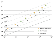
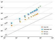
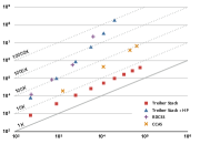
Figure 4. State-space reduction using $\approx$-quotienting.

All experiments run on a server which is equipped with a 4$\times$12-core AMD CPU @ $2.1$ GHz and $192$ GB memory under 64-bit Debian 7.6. Figure 4 shows the state-space savings for 11 algorithms (for two threads invoking methods for 2-10 times). Note that both the $x$- and the $y$-axis are in log-scale; for the sake of clarity we have indicated the lines with state space reduction factor 1 up to 10000 explicitly. Branching bisimulation quotient construction has yielded state-space savings of up to four orders of magnitude in the best cases, and to two to three orders for most cases. And in general, for the non-blocking implementation, the larger the system the higher the state space reduction factor. The largest reductions were obtained for the Treiber stack with hazard pointers (Treiber stack+HP) and the MS lock-free queue yielding a quotient with 0.01% and 0.02% of the size of the concrete objects, respectively. Verifying linearizability directly on the concrete state space would be practically infeasible.

6. Related Work

Linearizability has been intensively investigated in the literature. A comparison with all works goes outside the scope of this paper; instead, we focus on the closest related works.

A plethora of proof-based techniques has been developed for verifying linearizability. Most are based on rely-guarantee reasoning [29, 30, 18], or establishing simulation relations [3, 4, 26]. These techniques often involve identifying linearization points which is a manual non-trivial task. Of the more recent works, Liang et al. [18] propose a program logic tailored to rely-guarantee reasoning to verify complex algorithms. This method is applicable to a wide range of popular non-blocking algorithms but is restricted to certain types of linearization points. Challenging algorithms such as the Herlihy-Wing queue ([17] and [5]) fall outside this method. Our techniques do not rely on identifying linearization points, and are aimed to exploit established notions from concurrency theory.

Model checking methods to verify linearizability have been proposed in e.g., [21, 2, 32, 1]. Liu et al. [21] formalize linearizability as trace refinement and use partial-order and symmetry reduction techniques to alleviate the state explosion problem. Their experiments are limited to simple concurrent data structures such as counters and registers, and their technique is not applicable to checking progress properties. Cerny et al. [2] propose method automata to verify linearizability of concurrent linked-list implementations, which is restricted to two concurrent threads. An experience report with the model checker SPIN [32] introduces an automated procedure for verifying linearizability, but the method relies on manually annotated linearization points.

For the verification of progress properties, [11, 19, 20] recently propose refinement techniques with termination preservation. These techniques are limited to checking lock-freedom of some non-blocking algorithms (e.g., Treiber stack, MS and DGLM queues). Neither more complex non-blocking algorithms nor other progress properties are discussed. Our approach can check a large class of progress properties—in fact all properties expressible in CTL^∗ (containing LTL) without next. Our experiments treat 7 non-blocking algorithms and found a lock-free property violation in the revised stack [9]. Some formulations of progress properties using next-free LTL are discussed in [25, 7].

7. Conclusion

This paper proposed to exploit branching bisimulation (denoted $\approx$) — a well-established notion in the field of concurrency theory — for proving linearizability and progress properties of concurrent data structures. A concurrent object $O$ is linearizable w.r.t. a linearizable specification $\Theta_{sp}$ iff their quotients under $\approx$ are in a trace refinement relation. Unlike competitive techniques, this result is independent of the type of linearization points. If the abstract and concrete object are divergence-sensitive branching bisimilar, then progress properties of the — typically much smaller and simpler — abstract object carry over to the concrete object. This entails that progress properties such as lock- and wait-freedom (in fact all progress properties that can be expressed in the next-free fragment of CTL^∗) can be checked on the abstract program. Our approaches can be fully automated for finite-state systems. We have conducted experiments on 13 popular concurrent data structures yielding promising results. In particular, the fact that counterexamples can be obtained in an automated manner is believed to be a useful asset. Our experiments confirmed a known linearizability bug and revealed a new lock-free property violation.

Acknowledgement We thank the CADP support team for their helps and patience during the experiments.

Appendix A A Discussion on Weak Bisimulation

Weak bisimulation, $\approx_{w}$, is obtained by replacing the second clause of Definition 3.1 with:

1. if $s_{1}\xlongrightarrow{\tau}s_{1}^{\prime}$, then either ${(s_{1}^{\prime},s_{2})\in{\cal R}}$, or there exists $s^{\prime}_{2}$ such that $s_{2}\xLongrightarrow{}\xlongrightarrow{\tau}s_{2}^{\prime}$ and $(s_{1}^{\prime},s_{2}^{\prime})\in{\cal R}$.

Compared with branching bisimulation, weak bisimulation does not require the intermediate states passed through to be matched. We present an example showing that, because of this, weak bisimulation failed to preserve linearization points.

The example is Michael-Scott lock-free queue (MS queue) [23], shown in Figure 5. The queue is implemented by a linked-list, where Head and Tail refer to the first and the last node respectively. It provides two methods: (1) enq(v), which inserts an element in the end of the queue; and (2) deq, which removes the first element in the queue if there is one, and returns EMPTY otherwise.

• ⬇

  1 enq(v) {

  2 local x, t, s, b;

  3 x := cons(v, null);

  4 while (true) {

  5 t := Tail; s := t.next;

  6 if (t = Tail) {

  7 if (s = null) {

  8 b:=cas(&(t.next),s,x);

  9 if (b) {

  10 cas(&Tail,t,x);

  11 return; }

  12 }else cas(&Tail, t,s);

  13 }

  14 }

  15}
  ⬇

  16 deq() {

  17 local h, t, s, v, b;

  18 while (true) {

  19 h := Head; t := Tail;

  20 s := h.next;

  21 if (h = Head)

  22 if (h = t) {

  23 if (s = null)

  24 return EMPTY;

  25 cas(&Tail,t,s);

  26 }else {

  27 v := s.val;

  28 b:=cas(&Head,h,s);

  29 if(b) return v; }

  30 } }

Figure 5. The algorithm of MS lock-free queue.

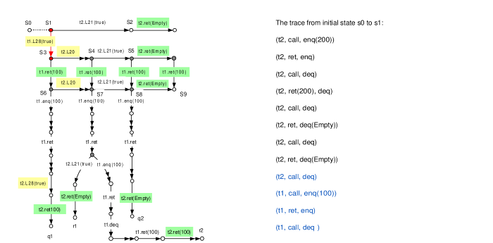
Figure 6. The (part) transition system for the MS lock-free queue.

Consider a system consisting of 2 client threads, each invoking methods enq(v) and deq 5 times. The transition system is partly depicted in Figure 6, where $s_{0}$ is the initial state, and $\twoheadrightarrow$ means $\xLongrightarrow{}$. The trace from $s_{0}$ to $s_{1}$ (shown in dotted line in the figure) is listed in text form on the right.

The transition $s_{1}\xlongrightarrow{\tau(t_{1}.L28)}s_{3}$ corresponds to a successful execution of $\mathtt{cas(Head,h,s)}$ removing an element from the queue, and is a linearization point of the call of deq by $t_{1}$.

Checking weak bisimulation with the CADP tool, it returns $s_{1}\approx_{w}s_{3}$, along with it $s_{2}\not\approx_{w}s_{4}$ and $s_{2}\approx_{w}s_{5}$. For branching bisimulation, the tool reports $s_{1}\not\approx s_{3}$, along with it $s_{2}\not\approx s_{4}$ and $s_{2}\approx s_{5}$.

To explain the difference, consider, for instance, the transition $s_{1}\xlongrightarrow{\tau}s_{2}$. In weak bisimulation, it can be matched by $s_{3}\xLongrightarrow{\tau}s_{4}\xlongrightarrow{\tau}s_{5}$, despite that $s_{2}\not\approx_{w}s_{4}$. However, this is not allowed in branching bisimulation because $s_{2}\not\approx s_{4}$.

References

- [1] Sebastian Burckhardt, Chris Dern, Madanlal Musuvathi, and Roy Tan. Line-up: A Complete and Automatic Linearizability Checker. In PLDI 2010, pages 330–340. ACM, 2010.
- [2] Pavol Cerný, Arjun Radhakrishna, Damien Zufferey, Swarat Chaudhuri, and Rajeev Alur. Model Checking of Linearizability of Concurrent List Implementations. In CAV 2010, LNCS vol.6174, pages 465–479. Springer, 2010.
- [3] Robert Colvin, Lindsay Groves, Victor Luchangco, and Mark Moir. Formal Verification of a Lazy Concurrent List-Based Set Algorithm. In CAV 2006, LNCS vol.4144, pages 475–488. Springer, 2006.
- [4] John Derrick, Gerhard Schellhorn, and Heike Wehrheim. Verifying Linearisability with Potential Linearisation Points. In FM 2011, LNCS vol.6664, pages 323–337. Springer, 2011.
- [5] Mike Dodds, Andreas Haas, and Christoph M. Kirsch. A scalable, correct time-stamped stack. In POPL 2015, pages 233–246, 2015.
- [6] Simon Doherty, Lindsay Groves, Victor Luchangco, and Mark Moir. Formal Verification of a Practical Lock-Free Queue Algorithm. In FORTE 2004, LNCS vol.3235, pages 97–114. Springer, 2004.
- [7] Brijesh Dongol. Formalising Progress Properties of Non-Blocking Programs. In ICFEM 2006, LNCS vol.4260, pages 284–303. Springer, 2006.
- [8] Ivana Filipovic, Peter W. O’Hearn, Noam Rinetzky, and Hongseok Yang. Abstraction for Concurrent Objects. Theor. Comput. Sci., 411(51-52):4379–4398, 2010.
- [9] Ming Fu, Yong Li, Xinyu Feng, Zhong Shao, and Yu Zhang. Reasoning about Optimistic Concurrency Using a Program Logic for History. In CONCUR 2010, LNCS vol.6269, pages 388–402. Springer, 2010.
- [10] Hubert Garavel, Frédéric Lang, Radu Mateescu, and Wendelin Serwe. CADP 2011: a toolbox for the construction and analysis of distributed processes. STTT, 15(2):89–107, 2013.
- [11] Alexey Gotsman and Hongseok Yang. Liveness-Preserving Atomicity Abstraction. In ICALP 2011, LNCS vol.6756, pages 453–465. Springer, 2011.
- [12] Jan Friso Groote and Frits W. Vaandrager. An Efficient Algorithm for Branching Bisimulation and Stuttering Equivalence. In ICALP 1990, LNCS vol.443, pages 626–638. Springer, 1990.
- [13] Jan Friso Groote and Anton Wijs. An o(m\log n) algorithm for stuttering equivalence and branching bisimulation. In TACAS 2016, pages 607–624, 2016.
- [14] Timothy L. Harris, Keir Fraser, and Ian A. Pratt. A Practical Multi-Word Compare-and-Swap Operation. In DISC 2002, LNCS vol.2508, pages 265–279. Springer, 2002.
- [15] Steve Heller, Maurice Herlihy, Victor Luchangco, Mark Moir, William N. Scherer III, and Nir Shavit. A Lazy Concurrent List-Based Set Algorithm. Parallel Processing Letters, 17(4):411–424, 2007.
- [16] Maurice Herlihy and Nir Shavit. The Art of Multiprocessor Programming. Morgan Kaufmann, 2008.
- [17] Maurice Herlihy and Jeannette M. Wing. Linearizability: A Correctness Condition for Concurrent Objects. ACM Trans. Program. Lang. Syst., 12(3):463–492, 1990.
- [18] Hongjin Liang and Xinyu Feng. Modular Verification of Linearizability with Non-Fixed Linearization points. In PLDI 2013, pages 459–470. ACM, 2013.
- [19] Hongjin Liang, Xinyu Feng, and Zhong Shao. Compositional Verification of Termination-Preserving Refinement of Concurrent Programs. In CSL-LICS 2014, page 65. ACM, 2014.
- [20] Hongjin Liang, Jan Hoffmann, Xinyu Feng, and Zhong Shao. Characterizing Progress Properties of Concurrent Objects via Contextual Refinements. In CONCUR 2013, LNCS vol.8052, pages 227–241. Springer, 2013.
- [21] Yang Liu, Wei Chen, Yanhong A. Liu, Jun Sun, Shao Jie Zhang, and Jin Song Dong. Verifying Linearizability via Optimized Refinement Checking. IEEE Trans. Software Eng., 39(7):1018–1039, 2013.
- [22] Maged M. Michael. Hazard Pointers: Safe Memory Reclamation for Lock-Free Objects. IEEE Trans. Parallel Distrib. Syst., 15(6):491–504, 2004.
- [23] Maged M. Michael and Michael L. Scott. Simple, Fast, and Practical Non-Blocking and Blocking Concurrent Queue Algorithms. In PODC 1996, pages 267–275, 1996.
- [24] Robin Milner. Communication and Concurrency. PHI Series in computer science. Prentice Hall, 1989.
- [25] Erez Petrank, Madanlal Musuvathi, and Bjarne Steensgaard. Progress Guarantee for Parallel Programs via Bounded Lock-Freedom. In PLDI 2009, pages 144–154. ACM, 2009.
- [26] Gerhard Schellhorn, Heike Wehrheim, and John Derrick. How to Prove Algorithms Linearisable. In CAV 2012, pages 243–259, 2012.
- [27] R.K. Treiber. Systems Programming: Coping with Parallelism. Research Report RJ 5118. IBM Almaden Research Center, 1986.
- [28] Aaron Joseph Turon, Jacob Thamsborg, Amal Ahmed, Lars Birkedal, and Derek Dreyer. Logical Relations for Fine-Grained Concurrency. In POPL 2013, pages 343–356. ACM, 2013.
- [29] Viktor Vafeiadis. Modular Fine-Grained Concurrency Verification. Technical Report UCAM-CL-TR-726, University of Cambridge, Computer Laboratory, July 2008.
- [30] Viktor Vafeiadis. Automatically Proving Linearizability. In CAV 2010, LNCS vol.6174, pages 450–464. Springer, 2010.
- [31] Rob J. van Glabbeek and W. P. Weijland. Branching Time and Abstraction in Bisimulation Semantics. J. ACM, 43(3):555–600, 1996.
- [32] Martin T. Vechev, Eran Yahav, and Greta Yorsh. Experience with Model Checking Linearizability. In SPIN 2009, LNCS vol.5578, pages 261–278. Springer, 2009.
- [33] Xiaoxiao Yang, Joost-Pieter Katoen, Huimin Lin, and Hao Wu. Proving linearizability via branching bisimulation (experimental report). URL: https://moves.rwth-aachen.de/wp-content/uploads/concur_2016_sub14_appendix.pdf.