On the Almost Global Stability of Invariant Sets*

Abstract

For a given invariant set of a dynamical system, it is known that the existence of a Lyapunov-type density function, called Lyapunov density or Rantzer’s density function, may imply the convergence of almost all solutions to the invariant set, in other words, the almost global stability (also called almost everywhere stability) of the invariant set. For discrete-time systems, related results in literature assume that the state space is compact and the invariant set has a local basin of attraction. We show that these assumptions are redundant. Using the duality between Frobenius-Perron and Koopman operators, we provide a Lyapunov density theorem for discrete-time systems without assuming the compactness of the state space or any local attraction property of the invariant set. As a corollary to this new discrete-time Lyapunov density theorem, we provide a continuous-time Lyapunov density theorem which can be used as an alternative to Rantzer’s original theorem, especially where the solutions are known to exist globally.

I Introduction

Stability of invariant sets of dynamical systems with respect to perturbations in initial conditions has always been a crucial topic in systems and control. A control task aims at global asymptotic stability of the invariant set under consideration, which will ensure the resilience of dynamic behaviour with respect to all changes in initial conditions. Recently, as an alternative to global asymptotic stability, a weaker notion called almost global stability (also called almost everywhere stability), which describes convergence of almost all solutions to the invariant set, has been introduced and found some applications in nonlinear analysis [1, 2, 3, 4, 5, 6] and control engineering [7, 8, 9]. The main idea was first introduced by Milnor [10], where a new notion of attractor is proposed as a minimal closed invariant set that attracts a set of positive measure. Milnor proved that if the state space is compact, there always exists a maximal attractor, called the likely limit set, which attracts almost all initial conditions. Obviously, if the state space is not compact, such a maximal attractor may not exist. A natural question along this line is to find sufficient conditions, even for systems with a non-compact state space, that ensure convergence of almost all solutions to a given invariant set, hence the almost global stability of the invariant set. Rantzer [11] introduced a dual Lyapunov approach to the almost global stability problem, where the existence of a density function, satisfying some Lyapunov-like conditions, is shown to imply almost global stability of an equilibria. This density function, called Lyapunov density or Rantzer’s density function, has been effectively applied to nonlinear feedback control [8] of continuous-time systems. For discrete-time systems, Vaidya and Mehta [3] use the Frobenius-Perron operator to provide a counterpart of Rantzer’s Lyapunov density theorem for invariant sets, assuming that the state space is compact and the invariant set is almost locally stable, namely that it attracts almost every point in some neighborhood of it. Using the same assumptions, a Lyapunov density theorem for invariant sets has been given for the continuous-time case in [12]. Also, the discrete-time Lyapunov density theorem in [3] has been applied to a feedback control design [9]. Using the Koopman operator, another approach for the global stability of nonlinear systems is given in [13, 14], which provides sufficient conditions for the global asymptotic stability of an equilibrium. Another related concept called occupation measure has been utilised in [15] for the convex computation of the region of attraction.

In this paper, we use the duality between Frobenius-Perron and Koopman operators (see [16] and [17] for the general theory of Markov processes where these operators appear) and provide a discrete-time version of Rantzer’s continuous-time density theorem [11] for invariant sets, that do not assume the compactness of the state space and the local stability of the invariant set . Subsequently, we use our theorem for discrete-time to prove a generalization of the continuous-time density theorem [11] to invariant sets . Both theorems require very similar sets of conditions for a Lyapunov density function, leading to a unification of the theories for discrete- and continuous-time systems, which we summarize below postponing the detailed descriptions for the more general statements of the theorems to Sections III and IV.

Let us consider a dynamical system on $\mathbb{R}^{n}$ given by

$$x^{+}(t)=F(x(t)),\ t\in\mathbb{T},$$ (1)

where the time set $\mathbb{T}$ is either $\mathbb{R}$ or $\mathbb{N}$, and $x^{+}(t):=\frac{dx(t)}{dt}$ if $\mathbb{T}=\mathbb{R}$ and $x^{+}(t):=x(t+1)$ if $\mathbb{T}=\mathbb{N}$. For $\mathbb{T}=\mathbb{N}$, we assume that $F$ is nonsingular. For $\mathbb{T}=\mathbb{R}$, we assume that $F$ is locally Lipschitz and that solutions of (1) uniquely exist for all time and for all initial conditions. As in [3] and [9], we use Frobenius-Perron operator ${\mathbb{P}}$ to characterize Lyapunov density in discrete-time. ${\mathbb{P}}$ captures the evolution of a distribution of initial states under the discrete-time dynamics. Similarly, the evolution of distributions in continuous-time is captured by the infinitesimal operator ${\mathbb{A}}$. Precise definitions for these operators will be given in the sequel. An invariant set $A\subset\mathbb{R}^{n}$ is said to be almost globally stable if there exists a subset $N\subset\mathbb{R}^{n}$ with zero Lebesgue measure such that $x(t)\to A$ as $t\to\infty$ for all $x(0)\in N^{c}$.

For an invariant set $A\subset\mathbb{R}^{n}$, we say that a continuously differentiable real function $\rho$ defined on $A^{c}$ is a Lyapunov density for $A$, if it is positive almost everywhere on $A^{c}$, integrable away from $A$ and properly subinvariant on $A^{c}$. Specifically, we say that $\rho$ is properly subinvariant on $A^{c}$ if $\mathbb{L}\rho(x)<0$ for almost all $x\in A^{c}$, where $\mathbb{L}\rho={\mathbb{P}}\rho-\rho$ for discrete time systems and $\mathbb{L}\rho={\mathbb{A}}\rho$ for continuous time systems.

Our main result can now be stated in a unified form for discrete- and continuous-time systems as follows:
Main result: A compact invariant set $A$ is almost globally stable if there exists a Lyapunov density for $A$.

Section II summarizes the required preliminary definitions and results on Frobenius-Perron operator, Koopman operator and their duality. The detailed descriptions and proofs of the main result for discrete time and continuous timme are given in Section III and Section IV, respectively. Finally, some illustrative examples of applications of the main result are provided in Section V.

II Preliminary Definitions and Tools

By a measure $\mu$ on $\mathbb{R}^{n}$, we mean a $\sigma$-finite measure defined on the Borel $\sigma$-algebra $\mathcal{B}$ of $\mathbb{R}^{n}$. In particular, Lebesgue measure on $\mathbb{R}^{n}$ will be denoted by $m$. A measure $\mu$ is said to be absolutely continuous (with respect to $m$) if $\mu(A)=0$ whenever $m(A)=0$.

We assume that the dynamics given by $T:\mathbb{R}^{n}\to\mathbb{R}^{n}$ is nonsingular; namely, $A\in{\mathcal{B}}$ and $m(A)=0$ implies that $m({T^{-1}}A)=0$.

The Radon-Nikodym theorem states that if $\mu$ is absolutely continuous then there exist a unique (modulo sets of zero Lebesgue measure) nonnegative measurable function $\rho$ such that

$$\mu(A)=\int_{A}\rho\ dm.$$ (2)

$\rho$ is called the Radon-Nikodym derivative of $\mu$ (with respect to $m$). On the other hand, if $\rho$ is a nonnegative measurable function then $\mu(A):=\int_{A}\rho\ dm$ defines an absolutely continuous measure on $\mathbb{R}^{n}$. Therefore, there is a one-to-one correspondence between the set of absolutely continuous measures on $\mathbb{R}^{n}$ and the set of equivalence classes of non-negative measurable functions on $\mathbb{R}^{n}$, where equivalence classes are defined as sets of functions that differs only on sets of zero Lebesgue measure. Both of these sets are denoted by $\mathcal{M}^{+}(\mathbb{R}^{n})$. Naturally, this extends to another equivalence between absolutely continuous signed measures on $\mathbb{R}^{n}$ and the set of equivalence classes of measurable functions on $\mathbb{R}^{n}$, both of which are denoted by $\mathcal{M}(\mathbb{R}^{n})$. In addition, the linear vector space of all signed measures on $\mathbb{R}^{n}$ is denoted by $\overline{\mathcal{M}}(\mathbb{R}^{n})$ and the space of equivalence classes of integrable functions on $\mathbb{R}^{n}$ is denoted by $\mathcal{L}_{1}(\mathbb{R}^{n})$. Note that $\overline{\mathcal{M}}(\mathbb{R}^{n})\supset\mathcal{M}(\mathbb{R}^{n})\supset\mathcal{L}_{1}(\mathbb{R}^{n})$.

II-A Frobenius-Perron Operator

The evolution of distributions under the discrete-time dynamics of (1) can be captured by a linear operator ${\mathbb{P}}:\overline{\mathcal{M}}(\mathbb{R}^{n})\to\overline{\mathcal{M}}(\mathbb{R}^{n})$ (called Frobenius-Perron operator) defined as

$$({\mathbb{P}}\mu)(A):=\mu({T^{-1}}A).$$ (3)

Assume that $\mu$ is absolutely continuous. Since $T$ is nonsingular

$$m(A)=0\implies m({T^{-1}}A)=0\\ \implies\mu({T^{-1}}A)=0\implies({\mathbb{P}}\mu)(A)=0$$ (4)

so ${\mathbb{P}}\mu$ is also absolutely continuous. Therefore, ${\mathbb{P}}$ maps $\mathcal{M}^{+}(\mathbb{R}^{n})$ to itself and similarly ${\mathbb{P}}$ maps $\mathcal{M}(\mathbb{R}^{n})$ to itself. For a nonnegative measurable function $\rho\in\mathcal{M}^{+}(\mathbb{R}^{n})$, ${\mathbb{P}}\rho$ is defined as the Radon-Nikodym derivative of ${\mathbb{P}}\mu$ with respect to $m$. Using (2) and (3), it follows that

$$\int_{A}{\mathbb{P}}\rho dm=\int_{{T^{-1}}A}\rho dm.$$ (5)

Substituting $A=\mathbb{R}^{n}$ in (5) implies that ${\mathbb{P}}$ maps integrable functions to integrable functions. Hence, the restriction of ${\mathbb{P}}$ to $\mathcal{L}_{1}(\mathbb{R}^{n})$, denoted by ${\mathbb{P}}|_{\mathcal{L}_{1}(\mathbb{R}^{n})}$, produces a map $\mathcal{L}_{1}(\mathbb{R}^{n})\to\mathcal{L}_{1}(\mathbb{R}^{n})$ which is a Markov operator. Namely, ${\mathbb{P}}={\mathbb{P}}|_{\mathcal{L}_{1}(\mathbb{R}^{n})}$ satisfies the following conditions:

$\rho\geq 0\implies{\mathbb{P}}\rho\geq 0$ and $\|{\mathbb{P}}\rho\|=\|\rho\|.$

II-B Koopman Operator

A dual method to capture the statistical behaviour of the deterministic system (1) is via the Koopman operator ${\mathbb{U}}$, which describes the evolution of the values of observables under the dynamics of (1). Define ${\mathbb{U}}:\mathcal{M}(\mathbb{R}^{n})\to\mathcal{M}(\mathbb{R}^{n})$ as

$$({\mathbb{U}}f)(x):=f(Tx).$$ (6)

Clearly, ${\mathbb{U}}$ is linear and maps positive functions to positive functions. It also maps bounded functions to bounded functions. Hence ${\mathbb{U}}$ can be restricted to $\mathcal{L}_{\infty}$, the normed vector space of equivalence classes of essentially bounded measurable functions.

II-C Duality between Frobenius-Perron and Koopman Operators

Let the scalar product $\langle\cdot,\cdot\rangle$ between $\mathcal{L}_{1}$ and $\mathcal{L}_{\infty}$ be defined by

$$\langle\rho,f\rangle:=\int\rho f\ dm,\quad\rho\in\mathcal{L}_{1},~{}~{}f\in\mathcal{L}_{\infty}.$$ (7)

Note that since $\rho\in\mathcal{L}_{1},~{}~{}f\in\mathcal{L}_{\infty}$, we have $\langle\rho,f\rangle\leq\text{ess}\sup f\int\rho dm<\infty$. The duality between ${\mathbb{P}}:\mathcal{L}_{1}\to\mathcal{L}_{1}$ and ${\mathbb{U}}:\mathcal{L}_{\infty}\to\mathcal{L}_{\infty}$ with respect to $\langle\cdot,\cdot\rangle$ can be seen by first observing that

$$\langle{\mathbb{P}}\rho,{1}_{A}\rangle=\int{\mathbb{P}}\rho 1_{A}\ dm=\int_{A}{\mathbb{P}}\rho\ dm=\int_{{T^{-1}}A}\rho\ dm\\ =\int\rho 1_{{T^{-1}}A}\ dm=\langle\rho,1_{{T^{-1}}A}\rangle=\langle\rho,{\mathbb{U}}1_{A}\rangle,$$ (8)

where $1_{A}$ denotes the characteristic function for $A\subset\mathbb{R}^{n}$. Since any function in $\mathcal{L}_{\infty}$ can be approximated by characteristic functions we have the following duality

$$\langle{\mathbb{P}}\rho,f\rangle=\langle\rho,{\mathbb{U}}f\rangle,\quad\rho\in\mathcal{L}_{1},\ f\in\mathcal{L}_{\infty}.$$ (9)

Remark 1

By (7) and (8), this duality persists even for general measurable functions when considering ${\mathbb{P}}$ and ${\mathbb{U}}$ as functions ${\mathcal{M}}(\mathbb{R}^{n})\to{\mathcal{M}}(\mathbb{R}^{n})$.

II-D An invariant set $A$ and ${\mathbb{P}}$ restricted to $A^{c}$

Let $A\subset\mathbb{R}^{n}$ be an invariant set of the dynamics $F$, that is $F(A)\subset A$. We observe that for any set $V\subset A^{c}$, $F^{-1}(V)\subset A^{c}$, ${\mathbb{P}}$ maps $\overline{\mathcal{M}}(A^{c})$ to itself. Moreover, since $A^{c}$ may not be invariant, the (restricted) operator ${\mathbb{P}}|_{A^{c}}$ may not be a Markov operator, but it is a sub-Markov operator, namely it satisfies the following conditions:

$\rho\geq 0\implies{\mathbb{P}}|_{A^{c}}\rho\geq 0$ and $\|{\mathbb{P}}|_{A^{c}}\rho\|\leq\|\rho\|$.

Let $A_{\varepsilon}$ denote the ${\varepsilon}$-neighborhood of $A$, namely $A_{\varepsilon}=\{x\in\mathbb{R}^{n}:\inf_{y\in A}d(x,y)<{\varepsilon}\}$, where $d$ denotes the standard metric on $\mathbb{R}^{n}$. We also write $A_{\varepsilon}^{c}$ for $(A_{\varepsilon})^{c}$. We say that $\rho\in\mathcal{M}^{+}(A^{c})$ is integrable away from $A$ if $\int_{A_{\varepsilon}}\rho(x)\;m(dx)$ is finite for all ${\varepsilon}>0$. $\rho\in\mathcal{M}^{+}(A^{c})$ is said to be properly subinvariant on $A^{c}$ if ${\mathbb{P}}|_{A^{c}}\rho(x)<\rho(x)$ for almost all $x\in A^{c}$.

III Discrete-Time Case

In this section, we consider almost global stability of an invariant set $A$ for a discrete-time system. In particular, we prove that $A$ is almost globally stable if there exists a density $\rho$ that is positive, integrable away from $A$ and properly subinvariant on $A^{c}$, that is, a discrete-time Lyapunov density as defined below. For the definitions of properly subinvariant density and integrability away from a subset, see the previous subsection.

We consider the dynamical system (1) with $\mathbb{T}=\mathbb{N}$ on a $\sigma$-finite measure space $(X,{\mathcal{B}},\mu)$ where $F$ is nonsingular. Throughout this section, we assume that $A\subset X$ is an invariant set for the system (1), ${\mathbb{P}}$ and ${\mathbb{U}}$ are the Frobenius-Perron and Koopman operators of the system (1) restricted to $A^{c}$, respectively.

Definition III.1 (Discrete-time Lyapunov density)

A measurable function $\rho$ defined on $A^{c}$ is called a discrete-time Lyapunov density for $A$ if it satisfies the following conditions:

• DLD1: $\rho$ is positive: $\rho(x)>0\ {\text{ for a.e. }}x\in A^{c}.$

• DLD2: $\rho$ is integrable away from $A$:

  $$\int_{A_{\varepsilon}^{c}}\rho(x)m(dx)<\infty\ \forall{\varepsilon}>0.$$ (10)

• DLD3: $\rho$ is properly subinvariant on $A^{c}$:

  $${\mathbb{P}}\rho(x)<\rho(x)\ {\text{ for a.e. }}x\in A^{c}.$$ (11)

This definition is less restrictive than the definition of a Lyapunov measure in [3], as it does not assume a local attraction property of the attractor. For discrete time systems the main result is the following:

Theorem III.2 (Almost global stability in discrete time)

An invariant set $A$ of the system (1) for $\mathbb{T}=\mathbb{N}$ is almost globally stable if there exists a discrete-time Lyapunov density for $A$.

Remark 2

In the language of attractor theory (see for instance [19] and the references therein), Theorem III.2 provides conditions for the existence of a maximal Milnor attractor for systems on noncompact spaces. Note that a maximal Milnor attractor, also called the likely limit set, always exists if the state space is compact [10].

Remark 3

For the case where $A^{c}$ is also invariant, ${\mathbb{P}}|_{A^{c}}$ is a Markov operator, namely it preserves the total mass of a measurable function $\rho$. This together with the proper subinvariance of $\rho$ implies that the Lyapunov density $\rho$ has infinite mass, namely it is not integrable. The nonintegrability of $\rho$ makes it difficult to approximate numerically with the methods in literature, such as the moment method for approximating finite measures [20].

We will use the following characterization for almost global stability of an invariant set $A$.

Lemma III.3

An invariant set $A$ is almost globally stable if and only if, for all ${\varepsilon}>0$, $\sum_{k=0}^{\infty}{\mathbb{U}}^{k}{\mathbb{1}}_{A_{\varepsilon}^{c}}(x)<\infty\ {\text{ for a.e. }}x$.

Proof:

Note that $T^{n}x\to A$ if and only if, for all ${\varepsilon}>0$, $\sum_{k=0}^{\infty}{\mathbb{U}}^{k}1_{A_{\varepsilon}^{c}}(x)<\infty$. In fact, $\sum_{k=0}^{\infty}{\mathbb{U}}^{k}1_{A_{\varepsilon}^{c}}(x)=\sum_{k=0}^{\infty}1_{A_{\varepsilon}^{c}}(T^{k}x)$ is equal to the number of visits of the trajectory $T^{n}x$ to the closed set $A_{\varepsilon}^{c}$. Hence, it is finite if and only if there exists an $N(\epsilon,x)>0$ such that $T^{n}(x)\in A_{\varepsilon}\ \forall n>N$. namely $T^{n}x\to A$.

By the above statement, the necessity is trivial. To prove the sufficiency, choose a sequence of positive numbers $\{{\varepsilon}_{n}\}\to 0$. By assumption, for each ${\varepsilon}_{n}$, $\sum_{k=0}^{\infty}{\mathbb{U}}^{k}{\mathbb{1}}_{A_{{\varepsilon}_{n}}^{c}}(x)<\infty\ {\text{ for a.e. }}x$, i.e. there exists a zero measure set $N_{{\varepsilon}_{n}}$ such that $\sum_{k=0}^{\infty}{\mathbb{U}}^{k}{\mathbb{1}}_{A_{{\varepsilon}_{n}}^{c}}(x)<\infty\ \forall x\in N_{{\varepsilon}_{n}}^{c}$. Let us define $N=\bigcup_{n}N_{{\varepsilon}_{n}}$. Obviously, $N$ has zero measure and we will show that, for all ${\varepsilon}>0$, $\sum_{k=0}^{\infty}{\mathbb{U}}^{k}{\mathbb{1}}_{A_{\varepsilon}^{c}}(x)<\infty\ \forall x\in N^{c}$. For a given ${\varepsilon}>0$, we can choose an $n$ such that ${\varepsilon}_{n}<{\varepsilon}$. Then, $\sum_{k=0}^{\infty}{\mathbb{U}}^{k}{\mathbb{1}}_{A_{\varepsilon}^{c}}(x)<\sum_{k=0}^{\infty}{\mathbb{U}}^{k}{\mathbb{1}}_{A_{{\varepsilon}_{n}}^{c}}(x)<\infty\ \forall x\in N^{c}$, since $N^{c}\subset N_{{\varepsilon}_{n}}^{c}$. ∎

We will also use the following basic fact to prove Theorem III.2:

Lemma III.4

Condition DLD3 implies that ${\text{ for a.e. }}x\in A^{c}$ $\lim_{n\to\infty}{\mathbb{P}}^{n}\rho(x)$ exists and is smaller than $\rho(x)$.

Proof:

Here, all arguments are valid ${\text{ for a.e. }}x\in A^{c}$. First note that ${\mathbb{P}}^{n}(\rho-{\mathbb{P}}\rho)\geq 0$, since ${\mathbb{P}}\rho<\rho$ and ${\mathbb{P}}^{n}$ is a positive operator for all $n$. Therefore, $0\leq{\mathbb{P}}^{n+1}\rho\leq{\mathbb{P}}^{n}\rho$ which implies that ${\mathbb{P}}^{n}\rho(x)$ is a decreasing sequence bounded from above by $\rho(x)$ and from below by $0$. Hence, the result follows. ∎

Proof:

By assumptions, there exists a measurable function $\rho>0$ such that $0<{\mathbb{P}}\rho<\rho$ and $\rho$ is integrable on $A_{\varepsilon}^{c}$ for every ${\varepsilon}>0$. Define $\rho_{0}:=\rho-{\mathbb{P}}\rho$. Clearly $\rho_{0}$ is positive $m$-a.e. and it follows that

$$\bar{\rho}_{0} := \lim_{n\to\infty}\sum_{k=0}^{n}{\mathbb{P}}^{k}\rho_{0}=\lim_{n\to\infty}\sum_{k=0}^{n}{\mathbb{P}}^{k}\left(\rho-{\mathbb{P}}\rho\right)$$

$$= \lim_{n\to\infty}\left(\sum_{k=0}^{n}{\mathbb{P}}^{k}\rho-\sum_{k=1}^{n+1}{\mathbb{P}}^{k}\rho\right)=\lim_{n\to\infty}\left(\rho-{\mathbb{P}}^{n+1}\rho\right)$$

$$= \rho-\lim_{n\to\infty}{\mathbb{P}}^{n+1}\rho.$$

By Lemma III.4, the above pointwise limits exist and $\lim{\mathbb{P}}^{n}\rho<\rho$ almost everywhere on $A^{c}$. Since $\rho$ is integrable on $A_{\varepsilon}^{c}$, $\lim{\mathbb{P}}^{n}\rho$ is also integrable on $A_{\varepsilon}^{c}$ by Lebesgue’s dominated convergence theorem. These imply that $\bar{\rho}_{0}$ is integrable on $A_{\varepsilon}^{c}$. Therefore, using Tonelli’s theorem with the counting measure on natural numbers and the duality between ${\mathbb{P}}$ and ${\mathbb{U}}$ (see Remark 1), we have

$$\infty > \langle\bar{\rho}_{0},1_{A_{\varepsilon}^{c}}\rangle=\sum_{k=0}^{\infty}\langle{\mathbb{P}}^{k}\rho_{0},1_{A_{\varepsilon}^{c}}\rangle$$

$$= \sum_{k=0}^{\infty}\langle\rho_{0},{\mathbb{U}}^{k}1_{A_{\varepsilon}^{c}}\rangle=\langle\rho_{0},\sum_{k=0}^{\infty}{\mathbb{U}}^{k}1_{A_{\varepsilon}^{c}}\rangle$$

Since $\rho_{0}$ is positive $m$-a.e., $\sum_{k=0}^{\infty}{\mathbb{U}}^{k}1_{A_{\varepsilon}^{c}}$ is finite $m$-a.e. and from Lemma III.3, $A$ is almost globally stable. Note that, although the last series may not be integrable it is measurable and the duality still works as discussed at the end of Subsection II-C. ∎

IV Continuous-Time Case

In this section, we consider almost global stability of an invariant set $A$ of the system (1) for $\mathbb{T}=\mathbb{R}$. Similarly to the discrete-time case, we prove that $A$ is almost globally stable if there exists a density $\rho$ defined on $A^{c}$ which is positive, properly subinvariant and integrable away from $A$.

We consider the system (1) with $\mathbb{T}=\mathbb{R}$ on a $\sigma$-finite measure space $(X,{\mathcal{B}},\mu)$ where $F$ is continuously differentiable and solutions to (1) exists for all initial conditions $x(0)$ and for all $t\geq 0$. We also assume that $A\subset X$ is a compact invariant set for the system (1), $\{{\mathbb{P}}_{t}\}$ is the semigroup of Frobenius-Perron operators of the system (1) restricted to $A^{c}$ and ${\mathbb{A}}$ is the infinitesimal operator of the continuous semigroup $\{{\mathbb{P}}_{t}\}$, namely ${\mathbb{A}}\rho=-\nabla(F\rho)$ [17]. Here $\rho\in C^{1}(A^{c},\mathbb{R}^{n})$, the set of continuously differentiable functions from $A^{c}$ to $\mathbb{R}^{n}$.

Since $F$ is continuously differentiable, it is locally Lipschitz, and therefore finite-time solutions of (1) vary continuously with respect to the initial states.

Definition IV.1 (Continuous-time Lyapunov density)

A $\rho\in C^{1}(A^{c},\mathbb{R}^{n})$ is called a continuous-time Lyapunov density for $A$ if it satisfies the following conditions:

• CLD1: $\rho$ is positive: $\rho(x)>0\ {\text{ for a.e. }}x\in A^{c}.$

• CLD2: $\rho$ is integrable away from $A$:

  $$\int_{A_{\varepsilon}^{c}}\rho(x)\mu(dx)<\infty\ \forall{\varepsilon}>0.$$ (12)

• CLD3: $\rho$ is properly subinvariant on $A^{c}$:

  $${\mathbb{A}}\rho(x)<0{\text{ for a.e. }}x\in A^{c}.$$ (13)

Recall that, if $\rho$ is continuously differentiable, ${\mathbb{A}}\rho=-\nabla(F\rho)$.

Theorem IV.2 (Almost global stability in continuous time)

An invariant compact set $A$ of the system (1) for $\mathbb{T}=\mathbb{R}$ is almost globally stable if there exists a continuous-time Lyapunov density for $A$.

Remark 4

The condition of being compact for $A$ can be substituted by being closed and that there exists a Lipschitz constant of $F$ on any arbitrarily small neighbourhood of $A$.

Remark 5

Theorem IV.2 generalizes Rantzer’s theorem for almost global stability of equilibria [11] to invariant sets with a slight change in the integrability assumption. In Rantzer’s theorem, $\frac{\rho\|F\|}{|x|}$ is assumed to be integrable away from $A$; whereas in Theorem IV.2, integrability of $\rho$ (away from $A$) is required along with the assumption that the solutions exist globally. Example V.2 below shows that for some systems a function $\rho$ may satisfy the latter condition but not the former. We note here that the version of Rantzer’s theorem (implied by its proof in [11]) that assumes the integrability of $\rho$ and the boundedness of $F/|x|$ is more conservative than Theorem IV.2, since the latter condition is only a sufficient condition for the global existence of solutions.

We restate the following lemma from [11]:

Lemma IV.3

Consider an open set $D\subset\mathbb{R}^{n}$. Let $F,\rho\in\mathbb{C}^{1}(D,\mathbb{R}^{n})$, where $\rho$ is integrable. Let $\phi_{t}(x_{0})$ be the solution at $x_{0}$ of the system (1) with $\mathbb{T}=\mathbb{R}$. For a measurable set $Z$, assume that $\phi_{\tau}(Z):=\{\phi_{\tau}(x)\mid x\in Z\}\subset D$ for all $\tau\in[0,t]$. Then

$$\int_{\Phi_{t}(Z)}\!\!\rho(x)dx-\int_{Z}\!\!\rho(x)dx=\int_{0}^{t}\int_{\Phi_{\tau}(Z)}\!\!\left[\nabla\cdot(F\rho)\right](x)dxd\tau,$$ (14)

This leads to the following lemma:

Lemma IV.4

Assume that $\rho$ is a continuous-time Lyapunov density for $A$ for the system (1), then for any $\tau>0$, $\rho$ is a discrete-time Lyapunov density for $A$ for the time-$\tau$ map $\phi_{\tau}$ of (1)

Proof:

Let $Z\subset A^{c}$ be a compact set contained in $A^{c}_{\varepsilon}$ for some ${\varepsilon}>0$. Choose a $T\in\mathbb{R}$.

Since $Z$ and $[-T,0]$ are compact sets and the flow map $\phi(t,x)\equiv\phi_{t}(x)\equiv\phi_{x}(t)$ is continuous in $t$ and $x$, the set $\phi([-T,0],Z)$ is compact. By the invariance of $A$, any trajectory $\phi_{t}(z)$, $z\in Z$ is outside $A$, therefore $A$ and $\phi([-T,0],Z)$ are disjoint. Since $\mathbb{R}^{n}$ is a normal space, there exists a neighborhood of $A$ that is disjoint from $\phi([-T,0],Z)$. Hence, there exists a $\bar{\varepsilon}>0$ such that $\phi_{\tau}(Z)\subset A^{c}_{\bar{\varepsilon}}$ for all $\tau\in[-T,0]$.

Now, we can apply Lemma IV.3 with $t=-T$ and $D=A^{c}_{\bar{\varepsilon}}$. Since $\nabla(F\rho)>0$ and $\int_{\phi_{-T}(Z)}\rho(x)dx=\int_{Z}{\mathbb{P}}\rho(x)dx$, (14) implies that $\int_{Z}{\mathbb{P}}\rho(x)dx<\int_{Z}\rho(x)dx$. Since $Z$ is an arbitrary compact subset of $A^{c}_{\varepsilon}$, ${\mathbb{P}}\rho(x)<\rho(x)$ for almost all $x\in A^{c}_{\varepsilon}$. Since ${\varepsilon}>0$ is also arbitrary, we have ${\mathbb{P}}\rho(x)<\rho(x)$ for almost all $x\in A^{c}$. ∎

Figure 1: Illustration of the proof of Theorem IV.2

We are now ready for the proof of Theorem IV.2:

Proof:

We pick a positive number $\tau$, and define a sequence $(\tau_{n}=\frac{\tau}{n})$. By Lemma IV.4, $\rho$ is a discrete-time Lyapunov density for the flow maps $\phi_{\tau_{n}}(x)$ for $n=1,2,\dots$. For each $n$, Theorem III.2 implies that there exists a set $N_{n}$ of zero measure such that $x\in(N_{n})^{\text{c}}$ implies $\phi_{k\tau_{n}}(x)\to A$ as $k\to\infty$. Define $N:=\bigcup_{n=1}^{\infty}N_{n}$, which has zero measure. Then, for any $n$ and for any $x\in N^{c}$, $\phi_{k\tau_{n}}(x)\to A$ as $k\to\infty$. Hence, for any $\epsilon_{1}>0$, there exits $M(n)$ such that for $k>M(n)$, $d(\phi_{k\tau_{n}}(x),A)<\epsilon_{1}$.

We will show that $\phi_{t}(x)\to A$ for all $x\in N^{c}$. For some $x\in N^{c}$, suppose that $\phi_{t}(x)$ does not converge to $A$ as $t\to\infty$. Then, there is $\epsilon_{2}>0$ and a sequence $({t}_{k})$ such that $\lim_{k\to\infty}{t}_{k}=\infty$, and $\phi_{{t}_{k}}(x)\in A_{{\varepsilon}_{2}}^{c}$. Pick ${\varepsilon}_{1}<{\varepsilon}_{2}$, a subsequence $(\underline{t}_{k})$ of $(k\tau)$ and a subsequence $(\overline{t}_{n})$ of $({t}_{n})$ such that $\overline{t}_{n}\in]\underline{t}_{n},\underline{t}_{n+1}[$, $\phi_{x}(\underline{t}_{n})\in A_{\epsilon_{1}}$. The situation is illustrated in Fig.1. Such subsequences can be chosen as $\lim_{k\to\infty}k\tau=\infty$ and for $k>M(1)$, $\phi_{x}(k\tau)\in A_{\epsilon_{1}}$.

Thanks to the continuity of the flow map, each of the times $\overline{t}_{k}$ can be decreased by $\overline{\delta}_{k}$ such that $\phi_{x}(\overline{t}_{k}-\overline{\delta}_{k})\in\partial A_{\epsilon_{2}}$, furthermore each of the times $\underline{t}_{k}$ can be increased by $\underline{\delta}_{k}$ such that $\phi_{x}(\underline{t}_{k}+\underline{\delta}_{k})\in\partial A_{\epsilon_{1}}$ and $\phi_{x}(t)\in A_{\epsilon_{2}}-A_{{\varepsilon}_{1}}$ for all $t\in]\underline{t}_{n}+\underline{\delta}_{n},\overline{t}_{n}-\overline{\delta}_{n}[$. Let us define $\underline{t}_{n}^{\prime}\equiv\underline{t}_{n}+\underline{\delta}_{n}$, and $\overline{t}_{n}^{\prime}\equiv\overline{t}_{n}-\overline{\delta}_{n}$.

Since $A$ is compact, the closure $\overline{A}_{\epsilon_{2}}$ is compact, and there is a Lipschitz constant of the vector field $F$ on $\overline{A}_{\epsilon_{2}}$. Hence, $\inf\{\overline{t}_{n}^{\prime}-\underline{t}_{n}^{\prime}\}>0$. Pick now $\tau_{m}\in\{\tau_{n}\}$ such that $\tau_{m}<\inf\{\overline{t}_{n}^{\prime}-\underline{t}_{n}^{\prime}\}$. Then there is an infinite sequence $(k_{n})\subset\mathbb{N}$ with $k_{n}\tau_{m}\in]\underline{t}_{n}^{\prime},\overline{t}_{n}^{\prime}[$ for each $n\in\mathbb{N}$, such that $\phi_{k_{n}\tau_{m}}\in A_{\epsilon_{2}}-A_{{\varepsilon}_{1}}$ for all $n$. But $\lim_{n\to\infty}d(\phi_{k_{n}\tau_{m}}(x),A)=0$; hence, we arrive at a contradiction. ∎

V Examples

In this section, we present examples for Theorem III.2 and Theorem IV.2. Example V.1 and Example V.2 are illustrative applications of the theory in one-dimensional case for discrete time and continuous time, respectively. Example V.2 also shows that a function $\rho$ may satisfy the integrability condition given in Theorem IV.2 but do not satisfy the integrability condition given in [11]. Finally, Example V.3 demonstrates an application of the theory to an invariant set which is a heteroclinic cycle.

Example V.1

Consider the discrete-time dynamical system defined on $\mathbb{R}$

$$x(k+1)=T(x(k)),$$ (15)

where $T$ is the functional inverse of $S(x)=x+\alpha x^{3}$ for some $\alpha>0$. Here, we consider the invariant set $A=\{0\}$. It is easy to check that $A$ is globally asymptotically stable (by drawing $T$ and cobwebbing). Let us define $\rho(x)=\frac{1}{|x|^{3}}$. Then, ${\mathbb{P}}\rho(x)=\rho(T^{-1}(x))/(dT(x)/dx)=\rho(S(x))\cdot(dS(x)/dx)=\frac{1+3\alpha x^{2}}{|x+\alpha x^{3}|^{3}}=\rho(x)\cdot\frac{1+3\alpha x^{2}}{(1+\alpha x^{2})^{3}}$. Here, $\rho$ is a Lyapunov density, since it is positive on $\mathbb{R}-A$, integrable away from $A$ and it satisfies ${\mathbb{P}}\rho(x)<\rho(x)$ on $\mathbb{R}-A$. The last inequality follows from $(1+\alpha x^{2})^{3}=1+3\alpha^{2}x^{4}+3\alpha x^{2}+\alpha^{3}x^{6}>1+3\alpha x^{2}$.

Example V.2

Consider the system

$$\dot{x}=-\text{sign}(x)\cdot|x|^{\alpha}(1-e^{-|x|}),$$ (16)

where $\alpha>1$. Here, we consider the invariant set $A=\{0\}$. Note that the solutions of (16) are well-defined for all time and for all initial conditions, since the right-hand side is locally Lipschitz and solutions are bounded ($\dot{x}$ and $x$ have different signs). $\rho(x)={|x|^{-\alpha}}$ is a Lyapunov density for (16), since $\nabla\cdot(F\rho)=\frac{d}{dx}\left({-\emph{sign}(x)(1-e^{-|x|})}\right)=e^{-|x|}>0$ outside $A$. Since $\alpha>1$, $\rho$ is integrable away from $A$. Hence, by Theorem IV.2, the equilibrium $A$ is almost globally stable for positive $\alpha$. Note that, $\rho\|F\|/|x|=\frac{(1-e^{-|x|})}{|x|}$ is not integrable away from $A$, therefore, it does not satisfy the integrability condition in [11].

Example V.3 (A heteroclinic attractor ([21]))

Consider the following perturbed Hamiltonian system on $\mathbb{R}^{2}$ (shown in Fig. 2):

$$\dot{x} =-y$$ (17a)

$$\dot{y} =x-x^{3}-{\varepsilon}y\left(v(x,y)-\frac{1}{4}\right),$$ (17b)

where $v(x,y)=\frac{2x^{2}-x^{4}+2y^{2}}{4}$ is the Hamiltonian for the system with ${\varepsilon}=0$.

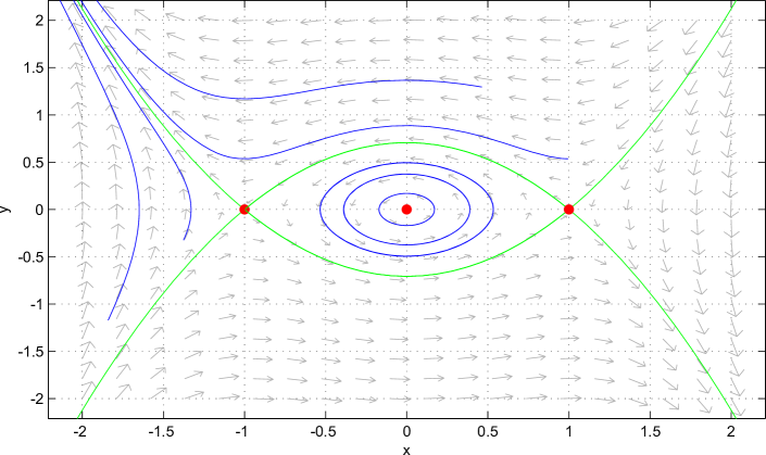
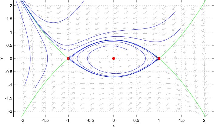
(a) $\epsilon=0$ (b) $\epsilon=1$

Figure 2: Heteroclinic trajectories (green), equilibrium points (red), and forward trajectories (blue) for the system given by (17)

For all ${\varepsilon}$, the system has three equilibria $p=(-1,0)$, $o=(0,0)$ and $q=(1,0)$. The equlibria $q$ and $p$ are contained in the level set $v(x,y)=\frac{1}{4}$. This level set also contains two heteroclinic trajectories connecting $p$ to $q$ and $q$ to $p$, forming a heteroclinic cycle, denoted by $A$, that persists for all ${\varepsilon}$. We consider the almost global stability of $A$. In [21], it is shown that $A$ attracts almost all initial points inside the cycle if ${\varepsilon}>0$ as stated . We will prove this by considering the Lyapunov density

$$\rho(x,y)=\frac{1}{\frac{1}{4}-v(x,y)}$$ (18)

Note that we consider the system on the invariant closed set $\overline{W}=W\cup A$, where $W$ is the sub-level set $v(x,y)<\frac{1}{4}$. To prove that the heteroclinic cycle $A$ is attracting for almost all initial conditions in $W$, observe that $\rho(x)>0$ for almost all $x\in W$ (LD1), $\rho$ is integrable on $W$ away from $A$ (LD2) and $\nabla\cdot(\rho F)>0$ almost everywhere on $W$ (LD3), since

$$\nabla\cdot(\rho F) = \nabla\cdot\begin{pmatrix}\frac{-y}{\frac{1}{4}-v(x,y)}\\ \frac{x-x^{3}-{\varepsilon}y(v(x,y)-\frac{1}{4})}{\frac{1}{4}-v(x,y)}\end{pmatrix}$$

$$= \frac{4y(-4x+4x^{3})}{{(1-2x^{2}+x^{4}-2y^{2})}^{2}}$$

$$+\frac{(4x-4x^{3})4y}{{(1-2x^{2}+x^{4}-2y^{2})}^{2}}+{\varepsilon}={\varepsilon}>0.$$

As an ending remark, we point out that this example is essentially a closed loop version of the cart-pole system (or swinging pendulum on a cart). Indeed, for this system the control task is to swing up and balance a pendulum attached to a cart by means of controlling the horizontal movement of the cart. The swing up phase is usually determined by a control strategy which makes the pendulum asymptotically approach to a heteroclinic cycle exactly as depicted in Fig. 2(b). In this case, Fig. 2(b) should be interpreted as the phase space $x=\theta$ and $y=\dot{\theta}$, with $\theta$ the angle locating the pendulum and the equilibria $q$ and $p$ having numerical values $(0,0)$ and $(\pi,0)$, respectively. For a detailed account we refer to [22, Chapter 3], and references therein.

VI Conclusion

We have presented a Lyapunov density theorem for discrete-time systems without assuming compactness of state space and local stability of the invariant set. We have also obtained a new continuous-time Lyapunov density theorem for systems with well-defined solutions on the whole time.

References

- [1] P. Monzon, “Almost global attraction in planar systems,” Sys. Contr. Lett., vol. 54, pp. 753–758, 2005.
- [2] ——, “Almost global stability of dynamical systems,” Ph.D. dissertation, Udelar, Uruguay, 2006.
- [3] U. Vaidya and P. G. Mehta, “Lyapunov measure for almost everywhere stability,” IEEE Transactions on Automatic Control, vol. 53, no. 1, pp. 307–323, 2008.
- [4] R. Potrie and P. Monzon, “Local implications of almost global stability,” Dynamical Systems, vol. 24, no. 1, pp. 109–115, 2009.
- [5] V. Grushkovskaya and A. Zuyev, “Attractors of nonlinear dynamical systems with a weakly monotonic measure,” Journal of Mathematical Analysis and Applications, vol. 422, pp. 559–570, 2015.
- [6] R. Rajaram and U. G. Vaidya, “Lyapunov density for coupled systems,” Applicable Analysis, vol. 94, no. 1, pp. 169–183, 2015.
- [7] A. Rantzer and F. Ceragioli, “Smooth blending of nonlinear controllers using density functions,” in Proceedings of the 2001 European Control Conference, 2001.
- [8] S. Prajna, P. A. Parrilo, and A. Rantzer, “Nonlinear control synthesis by convex optimization,” IEEE Transactions on Automatic Control, vol. 49, no. 2, pp. 310–314, 2004.
- [9] U. Vaidya, P. G. Mehta, and U. V. Shanbhag, “Nonlinear stabilization via control lyapunov measure,” IEEE Transactions on Automatic Control, vol. 55, no. 6, pp. 1314–1328, 2010.
- [10] J. Milnor, “On the concept of attractor,” Communications in Mathematical Physics, vol. 99, no. 2, pp. 177–195, jun 1985.
- [11] A. Rantzer, “A dual to Lyapunov’s stability theorem,” Systems and Control Letters, vol. 42, pp. 1–17, 2001.
- [12] R. Rajaram, U. Vaidya, M. Fardad, and B. Ganapathysubramanian, “Stability in the almost everywhere sense: A linear transfer operator approach,” Journal of Mathematical Analysis and Applications, vol. 368, no. 1, pp. 144–156, 2010.
- [13] A. Mauroy and I. Mezić, “A spectral operator-theoretic framework for global stability,” in Proceedings of the IEEE Conference on Decision and Control, 2013, pp. 5234–5239.
- [14] ——, “Global stability analysis using the eigenfunctions of the koopman operator,” arXiv:1408.1379, 2014.
- [15] D. Henrion and M. Korda, “Convex computation of the region of attraction of polynomial control systems,” IEEE Transactions on Automatic Control, vol. 59, no. 2, pp. 297–312, 2014.
- [16] S. R. Foguel, The Ergodic Theory of Markov Processes. New York: Van Nostrand Reinhold Company, 1969.
- [17] A. Lasota and M. C. Mackey, Chaos, Fractals and Noise: Stochastic Aspects of Dynamics. New York: Springer-Verlag, 1994.
- [18] G. Werner, Linear Algebra, 4th ed. Springer-Verlag, New York-Berlin, 1975, graduate Texts in Mathematics, No. 23.
- [19] Ö. Karabacak and P. Ashwin, “On statistical attractors and the convergence of time averages,” Mathematical Proceedings of the Cambridge Philosophical Society, vol. 150, no. 02, pp. 353–365, 2011.
- [20] J. B. Lasserre, Moments, Positive Polynomials and Their Applications, ser. Imperial College Press Optimization Series. Imperial College Press, London, 2010, vol. 1.
- [21] I. S. Labouriau and A. A. P. Rodrigues, “On Takens’ Last Problem: tangencies and time averages near heteroclinic networks,” ArXiv:1606.07017, 2016.
- [22] I. Fantoni and R. Lozano, Non-Linear Control for Underactuated Mechanical Systems. Springer-Verlag, New York, 2001.