Well-posed Bayesian Inverse Problems with Infinitely-Divisible and Heavy-Tailed Prior Measures

Abstract

We present a new class of prior measures in connection to $\ell_{p}$ regularization techniques when $p\in(0,1)$ which is based on the generalized Gamma distribution. We show that the resulting prior measure is heavy-tailed, non-convex and infinitely divisible. Motivated by this observation we discuss the class of infinitely divisible prior measures and draw a connection between their tail behavior and the tail behavior of their Lévy measures. Next, we use the laws of pure jump Lévy processes in order to define new classes of prior measures that are concentrated on the space of functions with bounded variation. These priors serve as an alternative to the classic total variation prior and result in well-defined inverse problems. We then study the well-posedness of Bayesian inverse problems in a general enough setting that encompasses the above mentioned classes of prior measures. We establish that well-posedness relies on a balance between the growth of the log-likelihood function and the tail behavior of the prior and apply our results to special cases such as additive noise models and linear problems. Finally, we discuss some of the practical aspects of Bayesian inverse problems such as their consistent approximation and present three concrete examples of well-posed Bayesian inverse problems with heavy-tailed or stochastic process prior measures.

1 Introduction

Gaussian prior measures are perhaps the most commonly used class of priors in infinite-dimensional Bayesian inverse problems. While the Gaussian class is very conveninet to use in both theory and practice, it has serious shortcomings in modelling of certain types of prior knowledge such as sparsity. In this article we introduce some non-Gaussian prior measures that are able to model parameters that are compressible or have jump discontinuities. We will discuss our goals in more detail after a brief introduction to the Bayesian framework for solution of inverse problems.

Consider the problem of estimating a parameter $u\in X$ from a set of measurements $y\in Y$ where both $X$ and $Y$ are Banach spaces and $y$ is associated with $u$ through a model of the form

(1) $$y=\tilde{\mathcal{G}}(u).$$

$\tilde{\mathcal{G}}$ is a generic stochastic mapping that models the relationship between the parameter and the observed data by taking the measurement noise into account (be it additive, multiplicative etc). As an example, if the measurement noise is additive then we can write

$$\tilde{\mathcal{G}}(u)=\mathcal{G}(u)+\eta$$

where $\mathcal{G}:X\mapsto Y$ is the (deterministic) forward model and $\eta$ is the (random) measurement noise which is independent of $u$. We want to estimate the parameter $u$ given a realization of $y$. Since the map $\mathcal{G}$ may not be stably invertible this problem is in general ill-posed.

Here we consider the Bayesian framework for solution of such ill-posed problems. Recall the infinite-dimensional version of Bayes’ rule [51] which is understood in the sense of the Radon-Nikodym theorem [8, Thm. 3.2.2]:

(2) $$\frac{\text{d}\mu^{y}}{\text{d}\mu_{0}}(u)=\frac{1}{Z(y)}\exp\left(-\Phi(u;y)\right)\quad\text{where}\quad Z(y)=\int_{X}\exp(-\Phi(u;y))\text{d}\mu_{0}(u).$$

Here $\mu_{0}$ is the prior measure which reflects our prior knowledge of the parameter $u$, $\Phi(u;y)$ is the likelihood potential that can be thought of as the negative log of the density of the data conditioned on the parameter $u$ and $\mu^{y}$ is the posterior measure on $u$. The posterior $\mu^{y}$ is, in essence, an updated version of the prior $\mu_{0}$ that is informed by the data $y$.

The Bayesian approach has attracted a lot of attention in the last two decades [13, 36, 51]. Put simply, the unknown parameter $u$ is modelled as a random variable and our goal is to obtain a probability distribution $\mu^{y}$ on $u$ that is informed by the data $y$ and our prior knowledge about $u$ (modelled by the measure $\mu_{0}$). We can generate samples from the posterior $\mu^{y}$ and if this measure is concentrated around the true value of the parameter, the sample mean or median will be good estimators of the true value of the parameter.

The Bayesian approach is well-established in the statistics literature [14, 5] where it is often applied in the setting where $X,Y$ are finite-dimensional spaces. Here we take $X$ to be an infinite-dimensional Banach space, motivation by applications where the parameter $u$ belongs to a function space such as $L^{2}$ or $BV$ (the space of functions with bounded variation). Such problems arise when the forward map involves the solution of a partial differential equation (PDE) or an integral equation such as the examples in Section 5.

In practice we solve these problems by discretizing the forward model and approximating the infinite-dimensional problem with a finite dimensional one. An important task is to ensure that the finite dimensional approximation to the posterior measure remains consistent with the infinite-dimensional posterior measure. For example, we require that the finite dimensional posterior converges to the (true) infinite-dimensional measure in the limit when the discretization is infinitely fine. Ensuring this consistency is a delicate task. An example of an inconsistent discretization of an infinite dimensional inverse problem was studied in [39] where the authors demonstrated that the total variation prior loses its edge preserving properties in the limit of fine discretizations. In order to resolve this issue we study the infinite-dimensional inverse problem before constructing the discrete approximations.

In this article we set out to achieve the following goals:

1. Construct a new class of infinitely divisible prior measures for recovery of compressible parameters in connection to $\ell_{p}$ regularization techniques when $p\in(0,1)$.

2. Present a systematic study of the class of infinitely divisible prior measures.

3. Introduce an alternative to the classic total variation prior using the laws of pure Jump Lévy process that is well-defined in infinite dimensions.

4. Present a theory of well-posedness for Bayesian inverse problems that encompasses the prior measures introduced under G1–G3.

Let us motivate some of these goals with an example.

Example 1.

Suppose $u\in\mathbb{R}^{n}$ and the data $y\in\mathbb{R}^{m}$ is generated via the model

$$y=\mathbf{A}u+\eta,\qquad\eta\sim\mathcal{N}(0,\sigma^{2}\mathbf{I})$$

where $\mathbf{A}\in\mathbb{R}^{n\times m}$, $\sigma>0$ is fixed and $\mathbf{I}$ is the $m\times m$ identity matrix. We wish to estimate $u$ given $y$. Here we are taking $X=\mathbb{R}^{n}$, $Y=\mathbb{R}^{m}$ and the forward map has the form $\mathcal{G}(u)=\mathbf{A}u$. Since $\eta$ has a Gaussian density we can write the likelihood potential $\Phi(u;y)$ as:

$$\Phi(u;y)=\frac{1}{2\sigma^{2}}\|\mathbf{A}u-y\|_{2}^{2}.$$

Then, Bayes’ rule gives

$$\frac{\text{d}\mu^{y}}{\text{d}\mu_{0}}(u)=\frac{1}{Z(y)}\exp\left(-\frac{1}{2\sigma^{2}}\|\mathbf{A}u-y\|_{2}^{2}\right).$$

Now define the prior measure via

(3) $$\frac{\text{d}\mu_{0}}{\text{d}\Lambda}(u)=\frac{1}{U}\exp\left(-\|u\|_{p}^{p}\right)$$

where $\text{d}\Lambda$ denotes the Lebesgue measure on $\mathbb{R}^{n}$, $\|\cdot\|_{p}$ denotes the usual $\ell_{p}$ (quasi-)norm in $\mathbb{R}^{n}$ for $p>0$ and $U$ is the appropriate normalizing constant. Then the posterior $\mu^{y}$ can be identified via its Lebesgue density as

(4) $$\frac{\text{d}\mu^{y}}{\text{d}\Lambda}(u)=\frac{1}{Z(y)}\exp\left(-\frac{1}{2\sigma^{2}}\|\mathbf{A}u-y\|_{2}^{2}-\|u\|_{p}^{p}\right).$$

The maximizer of the posterior density is referred to as the maximum a posteriori (MAP) estimate. Formally, the MAP estimate of the posterior in (4) is given by

$$u_{\text{MAP}}=\operatorname*{arg\,min}_{z\in\mathbb{R}^{n}}\left\{\frac{1}{2\sigma^{2}}\|\mathbf{A}z-y\|_{2}^{2}+\|z\|_{p}^{p}\right\}.$$

For $p\geq 1$ this optimization problem is convex and can be solved efficiently. Taking $p=1$ results in the well-known $\ell^{1}$-regularization technique which is often used in the recovery of sparse solutions. For values of $p\in(0,1)$ the resulting optimization problem is no longer convex but it is a good model for recovery of sparse or compressible solutions [26, 42].

It is straightforward to check that the prior distribution (3) for $p\in(0,1)$ is non-convex and heavy-tailed. However, we will see that this measure belongs to the much larger class of infinitely divisible measures. Formally, a random variable $\xi$ is infinitely-divisible if for every $n\in\mathbb{N}$ its law coincides with the law of $\sum_{k=1}^{n}\xi_{k}^{1/n}$ where $\{\xi_{k}^{1/n}\}$ are i.i.d. random variables. Thus, the above example is our first attempt at demonstrating the potential of infinitely-divisible prior measures (goals G1 and G2) that are introduced in Section 2. The connection between sparse recovery and heavy-tailed or infinitely divisible priors has been observed in the literature. Unser and Tafti [54] and Unser et al. [56, 55] study the sparse behavior of stochastic processes that are driven by infinitely divisible force terms and advocate their use in solution of inverse problems. A detailed discussion of some heavy-tailed prior distributions such as generalizations of the student’s-$t$ distribution and the $\ell_{p}$-priors can also be found in the dissertation [42]. Finally, Polson and Scott [47] and Carvalho et al. [16] propose a class of hierarchical horseshoe priors that are tailored to the recovery of sparse signals.

In practice, solving a Bayesian inverse problem often refers to either identifying the posterior measure $\mu^{y}$ (such as in (4)) or extracting certain statistics from it such as the mean, the variance, maximizer of the density etc. But before we can solve a Bayesian inverse problem we need to know whether the problem is well-posed to begin with (point G4 above): Does $\mu^{y}$ exist? Is it defined uniquely? Does it depend continuously on the data $y$? And finally, can we approximate it in a consistent manner?

Later on we see that the well-posedness of a Bayesian inverse problem relies on the type of prior measure $\mu_{0}$ that is chosen during the modelling step as well as certain properties of the potential $\Phi$. Well-posed Bayesian inverse problems were studied in [51, 20] with Gaussian prior measures, in [21] with Besov priors, in [34] with convex prior measures and in [22, 52] with heavy-tailed priors on separable Banach spaces. We note that our well-posedness results in this article are closely related to those of [22]. The main difference is that our theory does not rely on the assumption that the parameter space $X$ is separable and we impose slightly different conditions on the potential $\Phi$. The non-separability condition is particularly interesting when one takes $X$ to be $C^{\alpha}$(the space of Hölder continuous functions) or $BV$, neither of which are separable. In Section 3 we introduce a class of prior measures that are concentrated on $BV$ and have piecewise constant samples (goal G3). This example is later used in Section 5 as a prior measure in a deblurring problem.

1.1 Key definitions and notation

We gather here some key definitions and assumptions that are used in the remainder of the article. We let $\mathbb{R}_{+}$ denote the positive real line $[0,\infty)$ and use the shorthand notation $a\lesssim b$ when $a$ and $b$ are real valued functions and there exists an independent constant $C>0$ such that $a\leq Cb$. Given two random variables $\xi$ and $\zeta$ we use the notation $\xi\stackrel{{\scriptstyle d}}{{=}}\zeta$ to denote that they have the same laws (or distributions).

We use the shorthand notation $\{\gamma_{k}\}$ to denote a sequence of elements $\{\gamma_{k}\}_{k=1}^{\infty}$ in a vector space. The usual $\ell_{p}$ sequence spaces for $p\in[1,\infty]$ are defined as the space of real valued sequences $\{\gamma_{k}\}$ such that $\|\{\gamma_{k}\}\|_{p}<\infty$ where

$$\left.\begin{aligned} \|\{\gamma_{k}\}\|_{p}:=\left(\sum_{k=1}^{\infty}|\gamma_{k}|^{p}\right)^{1/p}\qquad\text{if}\qquad p\in[1,\infty)\qquad\text{and}\qquad\|\{\gamma_{k}\}\|_{\infty}:=\sup_{k}|\gamma_{k}|.\end{aligned}\right.$$

Similarly, we define the $\|\cdot\|_{p}$ norms of finite dimensional vectors. In particular $\|\cdot\|_{2}$ will denote the usual Euclidean norm. Given a positive definite matrix $\boldsymbol{\Sigma}$ of size $m\times m$, we define the norm

$$\|x\|_{\boldsymbol{\Sigma}}:=\|\Sigma^{-1/2}x\|_{2}\qquad\text{for}\qquad x\in\mathbb{R}^{m}.$$

Throughout the article we use $\Lambda$ to denote the Lebesgue measure in finite dimensions. Given a Borel measure $\mu$ on a Banach space $X$ we define the spaces $L^{p}(X,\mu)$ for $p\in[1,\infty)$ as the space of $\mu$-equivalent classes of functions $h:X\mapsto\mathbb{R}$ such that $|h|^{p}$ is $\mu$-integrable. We also use the shorthand notation $L^{p}(X)$ instead of $L^{p}(X,\Lambda)$ whenever we are working with the Lebesgue measure. Finally, if $X$ is a Banach space, we use $X^{\ast}$ to denote the topological dual of $X$ and $B_{X}(r)$ to denote the open ball of radius $r>0$ in $X$ that is centered at the origin. The shorthand notation $B_{X}$ denotes the unit ball.

We shall consider the prior probability measure $\mu_{0}$ to be in the class of Borel probability measures on $X$. In some cases we assume that the prior $\mu_{0}$ is Radon meaning that it is an inner regular probability measure on the Borel sets of $X$. Furthermore, whenever we say that $\mu$ is a probability measure on $X$ we automatically mean that $\mu(X)=1$. Finally, throughout this article we only consider complete probability measures in the following sense: If $\mu$ is a Borel probability measure on $X$ and $A$ is a set of $\mu$-measure zero then every subset of $A$ also has measure zero.

In this article we focus on the following notion of a well-posed Bayesian inverse problem:

Definition 1 (Well-posedness).

Suppose that $X$ is a Banach space and $d(\cdot,\cdot)\mapsto\mathbb{R}$ is a metric on the space of Borel probability measures on $X$. Then for a choice of the prior measure $\mu_{0}$ and the likelihood potential $\Phi$, the Bayesian inverse problem given by (2) is well-posed with respect to $d$ if:

1. (Existence and uniqueness) There exists a unique posterior probability measure $\mu^{y}\ll\mu_{0}$ given by Bayes’ rule (2).

2. (Stability) For every choice of $\epsilon>0$ there exists a $\delta>0$ so that $d(\mu^{y},\mu^{y^{\prime}})\leq\epsilon$ for all $y,y^{\prime}\in Y$ so that $\|y-y^{\prime}\|_{Y}\leq\delta$.

We will study the convergence of probability measures using the Hellinger and total variation metrics on the space of probability measures on $X$. For two probability measures $\mu_{1}$ and $\mu_{2}$ that are absolutely continuous with respect to a third measure $\nu$ on $X$, the total variation and Hellinger metrics are defined as

(5) $$d_{TV}(\mu_{1},\mu_{2}):=\frac{1}{2}\int_{X}\left|\frac{\text{d}\mu_{1}}{\text{d}\nu}-\frac{\text{d}\mu_{2}}{\text{d}\nu}\right|\text{d}\nu\quad\text{and}\quad d_{H}(\mu_{1},\mu_{2}):=\left(\frac{1}{2}\int_{X}\left(\sqrt{\frac{\text{d}\mu_{1}}{\text{d}\nu}}-\sqrt{\frac{\text{d}\mu_{2}}{\text{d}\nu}}\right)^{2}\text{d}\nu\right)^{1/2}.$$

Both metrics are independent of the choice of the measure $\nu$ [8, Lem. 4.7.35]. Furthermore, convergence in one of these metrics implies convergence in the other, due to the following inequalities (see [8, Lem. 4.7.37] for a proof)

(6) $$2d^{2}_{H}(\mu_{1},\mu_{2})\leq d_{TV}(\mu_{1},\mu_{2})\leq\sqrt{8}d_{H}(\mu_{1},\mu_{2}).$$

However, one might prefer to work with the Hellinger metric as it relates directly to the error in expectation of certain functions. Suppose that $h\in L^{2}(X,\mu_{1})\cap L^{2}(X,\mu_{2})$. Then using the Radon-Nikodym theorem and Hölder’s inequality one can show (see [34, Sec. 1] for details)

(7) $$\left|\int_{X}h(u)\text{d}\mu_{1}(u)\right.\left.-\int_{X}h(u)\text{d}\mu_{2}(u)\right|\leq 2\left(\int_{X}h^{2}(u)\text{d}\mu_{1}+\int_{X}h^{2}(u)\text{d}\mu_{2}\right)^{1/2}d_{H}(\mu_{1},\mu_{2}).$$

For reasons that will become clear in Section 4, we prefer to study the well-posedness of inverse problems using both the Hellinger and total variation metrics. The main difference is in the restrictions that we need to impose on the prior $\mu_{0}$ in order to obtain a certain rate of convergence for each metric.

2 Infinitely-divisible prior measures

We start by presenting a generalization of the prior distribution (3) that was considered in Example 1. We show that this prior belongs to a larger class of distributions that are closely related to $\ell_{p}$ regularization techniques. We shall extend these distributions to measures on Banach spaces with an unconditional Schauder basis and observe that they belong to the much larger class of infinitely-divisible (ID) measures (see Definition 9). Motivated by this connection between $\ell_{p}$ regularization and ID priors, we turn our attention to the ID class and discuss some of its properties. In particular, we study the tail behavior of ID priors with respect to their Lévy measures (see Definition 11).

2.1 A class of shrinkage priors with compressible samples

When faced with the problem of recovering a sparse or compressible parameter we require the prior measure to reflect the intuition that the solution to the inverse problem is likely to have only a few large modes in some basis and the rest of the modes are negligible (see [42, Sec. 6.1]). Such prior distributions are often referred to as “shrinkage priors” and they have been the subject of extensive research [47, 16, 28, 18, 17]. In this section we consider a few examples of shrinkage priors that are closely related to $\ell_{p}$ regularization techniques.

Most of the existing literature on shrinkage priors is focused on finite dimensional problems but we present an extension of these priors to infinite-dimensional Banach spaces. Since compressibility is often considered with respect to a basis, it makes sense for us to consider a parameter space that has a basis.

Given a parameter space $X$, or at least a subspace $\tilde{X}\subseteq X$ that has an unconditional Schauder basis $\{x_{k}\}$, we construct random variables of the form

(8) $$u\sim\sum_{k=1}^{\infty}\gamma_{k}\xi_{k}x_{k}$$

where $\{\gamma_{k}\}$ is a fixed sequence of real valued coefficients that decay sufficiently fast and the $\{\xi_{k}\}$ are a sequence of independent real valued random variables that need not be identically distributed. We will take the prior measure $\mu_{0}$ to be the law of the random variable $u$ in (8). We refer to such a prior measure $\mu_{0}$ as the product prior obtained from $\{\gamma_{k}\}$ and $\{\xi_{k}\}$. This construction of the prior is reminiscent of the Karhunen-Loéve expansion of Gaussian measures [7, Thm. 3.5.1]. The following theorem gives sufficient conditions that ensure $\|\cdot\|_{X}<\infty$ $\mu_{0}$-a.s.

Theorem 2.

[34, Thm. 3.9] Suppose that $X$ is a Banach space with an unconditional Schauder basis and let $u$ be as in (8). If $\{\gamma_{k}^{2}\}\in\ell_{p}$ and $\{\mathbf{Var}\xi_{k}\}\in\ell^{q}$ for $1<p,q<\infty$ so that $1/p+1/q=1$ (with $p=1$ for the limiting case when $q=\infty$), then $\|u\|_{X}<\infty$ a.s. In particular, if the $\{\xi_{k}\}$ are i.i.d., $\mathbf{Var}\xi_{1}<\infty$ and $\{\gamma_{k}\}\in\ell^{2}$, then $\|u\|_{X}<\infty$ a.s.

We can also show that the product prior $\mu_{0}$ that is induced by (8) is Radon. Proof of the next theorem follows the same approach as [34, Thm. 3.10(ii)] and is hence omitted.

Theorem 3.

Let $\mu$ be the probability measure that is induced by the random variable $u$ given by (8) where $\{\gamma_{k}\}$ and $\{\xi_{k}\}$ satisfy the conditions of Theorem 2. Then $\mu$ is a Radon probability measure on $X$ if the random variables $\{\xi_{k}\}$ are distributed according to Radon probability measures on $\mathbb{R}$.

Before going further we present a result on the second raw moment of product priors which will be useful throughout the remainder of the article.

Theorem 4.

Suppose that $X$ is a Banach space with an unconditional Schauder basis $\{x_{k}\}$ and let $\mu$ be the product prior obtained from $\{\gamma_{k}\}\in\ell^{2}$ and $\{\xi_{k}\}$ where $\xi_{k}$ are i.i.d. and $\mathbf{Var}\xi_{k}<\infty$. Then $\|\cdot\|_{X}\in L^{2}(X,\mu)$.

Proof.

Let $u_{N}=\sum_{k=1}^{N}\gamma_{k}\xi_{k}x_{k}$ then for $M>N>0$ we have

$$\left|\int_{X}\|u_{M}\|_{X}^{2}~{}\text{d}\mu-\int_{X}\|u_{N}\|_{X}^{2}~{}\text{d}\mu\right| =\left|\int_{X}(\|u_{M}\|_{X}-\|u_{N}\|_{X})(\|u_{M}\|_{X}+\|u_{N}\|_{X})~{}\text{d}\mu\right|$$

By Theorem 2 we know that $\|u\|_{X}<\infty$ a.s. and so in the limit as $M,N\mapsto\infty$, $|(\|u_{M}\|_{X}-\|u_{N}\|_{X})|\mapsto 2\|u\|_{X}$ and $|(\|u_{M}\|_{X}-\|u_{N}\|_{X})|\mapsto 0$ and so $\{\|u_{N}\|^{2}_{X}\}$ is Cauchy in $L^{2}(X,\mu)$. ∎

We are now in position to discuss a few examples of shrinkage priors. Motivated by Example 1, we define the class of $\ell_{p}$-priors as follows:

Definition 5 ($\ell_{p}$-prior).

Let $X$ be a Banach space with an unconditional Schauder basis $\{x_{k}\}$, then we say that a Radon probability measure $\mu$ is an $\ell_{p}$-prior on $X$ if its samples can be expressed as $u=\sum_{k=1}^{\infty}\gamma_{k}\xi_{k}x_{k}$ where $\{\gamma_{k}\}\in\ell^{2}$ and $\{\xi_{k}\}$ is an i.i.d. sequence of real valued random variables with Lebesgue density

(9) $$\xi_{k}\sim\frac{p}{2\alpha\Gamma(1/p)}\exp\left(-{\frac{|t|^{p}}{\alpha^{p}}}\right)\text{d}\Lambda(t)$$

where $p\in(0,\infty)$ and $\alpha=\sqrt{\Gamma(1/p)/\Gamma(3/p)}$.

Here $\Gamma$ denotes the usual Gamma function. The distribution in (9) belongs to the larger class of Generalized Normal distributions [44]. This class is also referred to as a Kotz-type distribution [43] or a generalized Laplace distribution [37]. Here we will not use either of these terms and simply refer to this distribution as the $\ell_{p}$-distribution to emphasize its connection to $\ell_{p}$-regularization techniques. The random variables $\xi_{k}$ have bounded moments of all orders (see [44] or the discussions following the definition of the $G_{p,q}$-prior below), in fact

$$\mathbb{E\>}\xi_{k}^{s}=\frac{\alpha^{s}(1+(-1)^{s})}{2\Gamma(1/p)}\Gamma\left(\frac{s+1}{p}\right)\qquad\text{for}\qquad s\in\mathbb{N}.$$

In particular we have that $\mathbf{Var}\xi_{k}=1$ and so it follows from Theorem 4 that the $\ell_{p}$-prior has bounded second moments.

Another, closely related class of priors to the $\ell_{p}$-priors can be obtained by a symmetrization of the Weibull distribution:

Definition 6 ($W_{p}$-prior).

Let $X$ be a Banach space with an unconditional Schauder basis $\{x_{k}\}$, then we say that a Radon probability measure $\mu$ is a $W_{p}$-prior on $X$ if its samples can be expressed as $u=\sum_{k=1}^{\infty}\gamma_{k}\xi_{k}x_{k}$ where $\{\gamma_{k}\}\in\ell^{2}$ and $\{\xi_{k}\}$ is an i.i.d. sequence of real valued random variables with Lebesgue density

(10) $$\xi_{k}\sim\frac{p}{\alpha}\left(\frac{|t|}{\alpha}\right)^{p-1}\exp\left(-\frac{|t|^{p}}{\alpha^{p}}\right)\text{d}\Lambda(t),$$

where $p\in(0,\infty)$ and $\alpha=(2\Gamma(1+2/p))^{-1/2}$.

The distribution of $\xi_{k}$ is simply a symmetric version of the well-known Weibull distribution [35], hence the name $W_{p}$. A straightforward calculation shows that $\mathbf{Var}\xi_{k}=1$ and once again it follows from Theorem 4 that the $W_{p}$-priors have bounded second moments.

Both the $W_{p}$ and $\ell_{p}$ distributions reduce to the Laplace distribution when $p=1$. For $p<1$ the $\ell_{p}$ distribution has non-convex level sets and puts a large portion of its mass close to the axes (see Figure 1). This behavior becomes stronger for smaller $p$ and suggests that the $\ell_{p}$-prior will incorporate sparse behavior as $p\mapsto 0$.

The $W_{p}$ distribution behaves very differently in comparison to the $\ell_{p}$ distribution. For $p<1$ the $W_{p}$ distribution blows up at the origin (see Figure 1(a)). This means that the $W_{p}$ distribution puts more of its mass at the origin which leads us to believe that it must incorporate stronger compressibility than the $\ell_{p}$ distribution.

Further insight into the behavior of the $W_{p}$-prior can be obtained by considering its MAP point estimate in finite dimensions. Formally, using this prior in Example 1 gives rise to an optimization problem of the form

$$u_{\text{MAP}}=\operatorname*{arg\,min}_{z\in\mathbb{R}^{n}}\left\{\frac{1}{2}\|\mathbf{A}z-y\|_{2}^{2}+\|z\|_{p}^{p}+(1-p)\sum_{k=1}^{n}\log(|z_{k}|)\right\}.$$

Of course, the $\log$ term on right hand side is not bounded from below and so we cannot gain much insight from this problem. However, we can consider a slightly modified version of this optimization problem by introducing a small parameter $\epsilon>0$

$$u_{\epsilon}=\operatorname*{arg\,min}_{z\in\mathbb{R}^{n}}\left\{\frac{1}{2}\|\mathbf{A}z-y\|_{2}^{2}+\|z\|_{p}^{p}+(1-p)\sum_{k=1}^{n}\log(\epsilon+|z_{k}|)\right\}.$$

Now if $\epsilon$ is small then the $\log$ term will heavily penalize any modes of the solution that are on a larger scale than that of $\epsilon$ and so we expect that most of the modes of the solution $u_{\epsilon}$ will be on the scale of the small parameter $\epsilon$. The stronger shrinkage of the posterior due to the $W_{p}$-prior is also evident in Figure 2 where we compare a prototypical example of posteriors that arise from the $W_{p}$ and $\ell_{p}$ priors for solution of Example 1 in 2D. Here, we clearly see that the $W_{1/2}$-prior results in a posterior that is highly concentrated around the axes compared to the posterior that arises from $\ell_{1/2}$-prior which is more spread out. Note that in either case, the posteriors are highly concentrated around the axes meaning that the map estimates as well as most of the samples from these posteriors will incorporate sparsity.

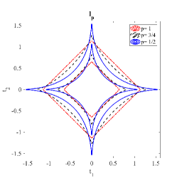
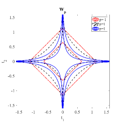
Fig. 1: Contour plots of $\ell_{p}$ and $W_{p}$ densities in 2D for different values of $p$.

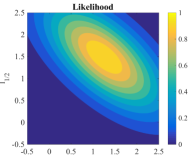
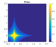
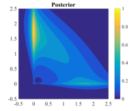
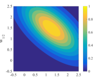
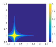
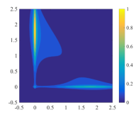
Fig. 2: A prototypical example of densities that arise in the solution of Example 1 in 2D with the $\ell_{1/2}$ (top row) and $W_{1/2}$ priors (bottom row). From left to right columns: The likelihood that arises from the additive Gaussian noise model, the prior densities and the resulting posteriors. The densities are rescaled for better visualization.

Comparing the distributions (9) and (10) suggests the definition of a larger class of priors that can interpolate between the $\ell_{p}$ and $W_{p}$-priors. To this end, we introduce a new class of prior measures called the $G_{p,q}$-priors. The letter $G$ is chosen due to the connection of the one dimensional version of these measures to the generalized Gamma distribution [10].

Definition 7 ($G_{p,q}$-prior).

Let $X$ be a Banach space with an unconditional Schauder basis $\{x_{k}\}$, then we say that a Radon probability measure $\mu$ is a $G_{p,q}$-prior on $X$ if its samples can be expressed as $u=\sum_{k=1}^{\infty}\gamma_{k}\xi_{k}x_{k}$ with $\{\gamma_{k}\}\in\ell^{2}$ and $\{\xi_{k}\}$ is an i.i.d. sequence of real valued random variables with Lebesgue density

(11) $$\xi_{1}\sim\frac{p}{2\alpha\Gamma(q/p)}\left|\frac{t}{\alpha}\right|^{q-1}\exp\left(-\left|\frac{t}{\alpha}\right|^{p}\right)d\Lambda(t),$$

where $p\in(0,\infty)$ and $\alpha=(\Gamma(q/p)/\Gamma((2+q)/p))^{1/2}$.

Using the change of variables $s=\frac{t^{p}}{\beta^{p}}$ we see that for $k,\beta\geq 0$

$$\int_{0}^{\infty}t^{k}\left(\frac{t}{\beta}\right)^{q-1}\exp\left(-\left(\frac{t^{p}}{\beta^{p}}\right)\right)d\Lambda(t)=\frac{\beta}{p}\int_{0}^{\infty}s^{\frac{k+q}{p}-1}\exp\left(-s\right)d\Lambda(s)=\frac{\beta^{k+1}}{p}\Gamma\left(\frac{k+q}{p}\right).$$

Setting $k=0$ leads us to the normalizing constant in the definition of the distribution in (11). Furthermore, we obtain the following expression for the moments of the $G_{p,q}$ distributions

$$\mathbb{E\>}|\xi_{1}|^{s}=\frac{\alpha^{s}(1+(-1)^{s})\Gamma\left((s+q)/p\right)}{2\Gamma\left(q/p\right)}\qquad s\in\mathbb{N}.$$

In particular $\mathbf{Var}\xi_{1}={\alpha^{2}\Gamma((2+q)/p)/\Gamma(q/p)}=1.$ Clearly, the $\ell_{p}$ prior is equivalent to $G_{p,1}$ and $W_{p}$ is equivalent to $G_{p,p}$. Furthermore, the $G_{1,q}$ distribution coincides with a symmetrization of the the Gamma distribution. For $q<1$ the distribution (11) will blow up at the origin and so it will put a lot of its mass at zero. The $G_{p,q}$ distributions belong to the class of ID measures by the following theorem of Bondesson.

Theorem 8 ([10, Cor. 2]).

All probability density functions on $(0,\infty)$ of the form

$$\pi(t)=\frac{p}{\alpha\Gamma(q/p)}\left(\frac{t}{\alpha}\right)^{q-1}\exp\left(-\left(\frac{t}{\alpha}\right)^{p}\right)$$

are ID for $q,\alpha>0$ and $0<p\leq 1$.

Later on we show that if the $\xi_{k}$ are distributed according to an ID distribution then the corresponding product prior on $X$ will also be an ID probability measure. Then the $G_{p,q}$-priors are also ID. This fact suggests the question of what other types of ID measures are good models for compressibility? We know that heavy-tailed distributions such as the Cauchy or Student’s t distributions are ID and they incorporate compressible samples as well. Then there is much to be gained from the study of ID prior measures in Bayesian inverse problems. To the best of our knowledge a thorough study of the compressible behavior of ID distributions is still missing in the literature. The closest reference in this direction is the works of Unser et. al. [54, 56, 55]. While we do not study the modelling of compressible parameters, we recognize the potential impact of ID priors in this subject and so we dedicate the remainder of this section to the study of ID priors.

2.2 Infinitely divisible priors

We begin by collecting some results on the class of ID probability measures on Banach spaces. We only present the results that are needed in our exposition and refer the reader to [41] for a detailed introduction to ID measures on Banach spaces. Further reading can be found in the monograph [54] which contains a modern treatment of ID probability measures on nuclear spaces and the books [3, 49, 50] that are good references on the theory of ID measures in finite dimensions.

Recall that given a Borel probability measure $\mu$ on a Banach space $X$ its characteristic function $\hat{\mu}:X^{\ast}\mapsto\mathbb{C}$ is given by

$$\hat{\mu}(\varrho)=\int_{X}\exp(i\varrho(u))\text{d}\mu(u)\qquad\forall\varrho\in X^{\ast}.$$

Characteristic functions play a crucial role in our discussion of ID measures in this section. In what follows $\nu^{\ast n}$ denotes the $n$-fold convolution of a measure $\nu$ with itself.

Definition 9 (ID measures [41]).

A Radon probability measure $\mu$ on a Banach space $X$ is called an infinitely divisible measure if for each $n\in\mathbb{N}$ there exists a Radon probability measure $\mu_{1/n}$ so that $\mu=(\mu_{1/n})^{\ast n}.$ Equivalently, the probability measure $\mu$ is ID if $\hat{\mu}(\varrho)=(\hat{\mu}_{1/n}(\varrho))^{n},\forall\varrho\in X^{\ast}.$

Put simply, a real valued random variable $\xi$ is distributed according to an ID measure if for every $n\in\mathbb{N}$ one can find a collection of i.i.d. random variables $\{\xi_{k}\}_{k=1}^{n}$ so that $\xi\stackrel{{\scriptstyle d}}{{=}}\sum_{k=1}^{n}\xi_{k}$. Examples of such distributions include Gaussian, Laplace, Gamma, log-normal, Cauchy and Student’s-t. More examples can be found in the monograph [50] where ID distributions on $\mathbb{R}$ are studied in detail. We note that an equivalent definition of an ID measure is given as the law of a Lévy process terminated at unit time. However, we will not use this definition in order to avoid the technicalities of dealing with Lévy processes but instead we refer the interested reader to the monographs [46, 19] for further reading. The proof of the next theorem can be found in [41, Sec. 5.1].

Theorem 10.

Let $\mu$ be an ID probability measure on a Banach space $X$. Then

1. $\hat{\mu}(\varrho)\neq 0$ for all $\varrho\in X^{\ast}$.

2. There exists a unique and continuous (in the dual norm) function $\psi:X^{\ast}\mapsto X$ so that $\hat{\mu}(\varrho)=\exp(\psi(\varrho))$ and $\psi(0)=0$.

3. If $\mu$ is symmetric, i.e. $\mu(A)=\mu(-A)$ for all Borel subsets $A$ of $X$, then $\hat{\mu}$ is real valued and positive.

4. For every $n\in\mathbb{N}$ the measures $\mu_{1/n}$ are uniquely determined and $\hat{\mu}_{1/n}(\varrho)=\exp(n^{-1}\psi(\varrho))$ for all $\varrho\in X^{\ast}$.

Furthermore, we define the function

$$\Psi(u,\varrho):=\exp(i\varrho(u))-1-i\varrho(u)\mathbf{1}_{B_{X}}(u)\qquad\forall u\in X,\varrho\in X^{\ast},$$

where $B_{X}$ is the unit ball in $X$ and $\mathbf{1}_{B_{X}}$ is the characteristic function of the unit ball. We recall the definition of a Lévy measure on a Banach space.

Definition 11 (Lévy Measure).

A positive $\sigma$-finite Radon measure $\lambda$ on $X$ is called a Lévy measure if and only if

1. $\lambda(\{0\})=0$.

2. $\int_{X}|\Psi(u,\varrho)|\text{d}\lambda(u)<\infty$ for every $\varrho\in X^{\ast}$.

3. $\exp(\int_{X}\Psi(u,\varrho)\text{d}\lambda(u))$ is the characteristic function of a Radon probability measure on $\mathbb{R}$ for every $\varrho\in X^{\ast}$.

We are now ready to present the celebrated Lévy-Khintchine representation theorem (see [41, Sec. 5.7] for a proof):

Theorem 12 (Lévy-Khintchine representation).

A Radon probability measure on a Banach space $X$ is infinitely divisible if and only if there exists an element $m\in X$, a (positive definite) covariance operator $\mathcal{R}:X^{\ast}\mapsto X$ and a Lévy measure $\lambda$, so that

(12) $$\hat{\mu}(\varrho)=\exp(\psi(\varrho))\quad\text{where}\quad\psi(\varrho)=i\varrho(m)-\frac{1}{2}\varrho(\mathcal{R}(\varrho))+\int_{X}\Psi(u,\varrho)\text{d}\lambda(u).$$

Equivalently, $\mu$ is ID precisely when there exists a point mass $\delta_{m}$, a Gaussian measure $\mathcal{N}(0,\mathcal{R})$ and a Radon measure $\nu$ identified via $\hat{\nu}(\varrho)=\int_{X}\Psi(u,\rho)\text{d}\lambda(u)$ so that

(13) $$\mu=\delta_{m}\ast\mathcal{N}(0,\mathcal{R})\ast\nu.$$

The Lévy-Khintchine representation implies that the triple $(m,\mathcal{R},\lambda)$ completely identifies an ID measure $\mu$ and so we use the shorthand notation $\mu=\text{ID}(m,\mathcal{R},\lambda)$. To gain more insight into the implications of the Lévy-Khintchine representation we recall the class of compound Poisson random variables and their corresponding probability measures.

Definition 13 (Compound Poisson probability measure [41, Sec. 5.3]).

Let $\eta$ be a Radon probability measure on a Banach space $X$ and suppose that $\{u_{k}\}$ is a sequence of i.i.d. random variables so that $u_{k}\sim\eta$. Also, let $\tau$ be an independent Poisson random variable with rate $c>0$ taking values in $\mathbb{Z}_{+}$. Then $u=\sum_{k=0}^{\tau}u_{k}$ is distributed according to a compound Poisson probability measure denoted by $\text{CPois}(c,\eta)$.

It is straightforward to check that the characteristic function of a compound Poisson measure has the form

$$\widehat{\text{CPois}(c,\eta)}(\varrho)=\exp\left(c\int_{X}(\exp(i\varrho(u))-1)\>\text{d}\eta(u)\right)\qquad\forall\varrho\in X^{\ast}.$$

See [41, Prop. 5.3.1] for a proof of this formula along with the fact that $\text{CPois}(c,\eta)$ is a Radon measure on $X$.

Now let us return to the characteristic function of the probability measure $\nu$ that was introduced in the Lévy-Khintchine representation (13)

(14) $$\begin{split}\hat{\nu}(\varrho)&=\exp\left(\int_{X}(\exp(i\varrho(u))-1)\>\text{d}\lambda(u)\right)\exp\left(\int_{B_{X}}-i\varrho(u)\>\text{d}\lambda(u)\right).\end{split}$$

If $0<\lambda(X)<\infty$ then $\lambda$ can be renormalized to define a probability measure $\tilde{\lambda}:=\frac{1}{\lambda(X)}\lambda$. Furthermore, we can define an element $u_{\lambda}\in X$ so that

$$\varrho(u_{\lambda})=-\int_{X}\varrho(u)\mathbf{1}_{B_{X}}(u)\text{d}\lambda(u)\qquad\forall\varrho\in X^{\ast}.$$

Putting these observations together with (14) gives the decomposition

(15) $$\nu=\text{CPois}(\lambda(X),\tilde{\lambda})\ast\delta_{u_{\lambda}}.$$

Therefore, from (13) we deduce that any measure $\mu=\text{ID}(m,\mathcal{R},\lambda)$ with $\lambda(X)<\infty$ can be decomposed as

(16) $$\mu=(\delta_{m+u_{\lambda}})\ast\mathcal{N}(0,\mathcal{R})\ast\text{CPois}(\lambda(X),\tilde{\lambda}).$$

In the remainder of this article we will restrict our attention to the case of ID measures with $\lambda(X)<\infty$. Since the tail behavior of prior measures is of importance to our well-posedness results in Section 4 we now present some results concerning the tail behavior of ID measures. We begin with the notion of a submultiplicative function.

Definition 14 (Submultiplicative function).

A non-negative, non-decreasing and locally bounded function $h:\mathbb{R}\mapsto\mathbb{R}^{+}$ is called submultiplicative if it satisfies

$$h(t+s)\leq Ch(t)h(s)\qquad\forall t,s\in\mathbb{R}$$

with an independent constant $C>0$

Our interest in the class of submultiplicative functions arises from the next theorem that describes some of the properties of this class.

Theorem 15 ([49, Prop. 25.4]).

1. The product of two submultiplicative functions is also submultiplicative.

2. If $h$ is submultiplicative then so is $(h(at+b))^{\alpha}$ for constants $a,b\in\mathbb{R}$ and $\alpha>0$.

3. The functions $\max\{1,|t|\}$ and $\exp(|t|^{\beta})$ for $\beta\in(0,1)$ are submultiplicative.

We now present a theorem that relates the tail behavior of an ID measure to that of its Lévy measure. This result was originally proven by Kruglov [38] for ID random variables on $\mathbb{R}$ with Lévy measures that are not necessarily finite. Different generalizations of this result to larger spaces are also available in the literature. For example, see [49, Thm. 25.3] for extension to $\mathbb{R}^{n}$ and [46, Prop. 6.9] for Hilbert space valued Lévy processes. For the reader’s convenience we briefly prove this result for Banach space valued ID random variables with finite Lévy measures.

Theorem 16.

Let $X$ be a Banach space and $\lambda$ be a Lévy measure so that $0<\lambda(X)<\infty$. Suppose that $u\sim\mu=\text{ID}(m,\mathcal{R},\lambda)$, $\mu(X)=1$ and $\|\cdot\|_{X}<\infty$ $\mu$-a.s. Then, given a submultiplicative function $h$ we have that $h(\|\cdot\|_{X})\in L^{1}(X,\mu)$ if $h(\|\cdot\|_{X})\in L^{1}(X,\lambda)$.

Proof.

Let $u\sim\mu$, then following Theorem 12 and the decomposition (16) above, we know that there exists an element $\tilde{m}\in X$ and independent random variables $w\sim\mathcal{N}(0,R)$ and $v\sim\text{CPois}(\lambda(X),\frac{1}{\lambda(X)}\lambda)$ so that

$$\mathbb{E\>}h(\|u\|_{X})=\mathbb{E\>}h(\|\tilde{m}+w+v\|_{X})\leq C^{3}h(\|\tilde{m}\|_{X})(\mathbb{E\>}h(\|w\|_{X}))(\mathbb{E\>}h(\|v\|_{X}))$$

where the inequality follows because of the triangle inequality and the fact that $h$ is non-decreasing and locally bounded. Now by [49, Lem. 25.5] we know that there exist constants $a,b>0$ such that $h(x)\leq b\exp(a|x|)$. Using this bound with the assumption that $\|u\|_{X}<\infty$ $\mu$-a.s. along with Fernique’s theorem [7, Thm. 2.8.5] for Gaussian measures on Banach spaces implies that $\mathbb{E\>}h(\|w\|_{X})<\infty$. Now suppose that $\frac{1}{\lambda(X)}\int_{X}h(\|u\|_{X})\text{d}\lambda(u)=U<\infty$. Then using the law of total expectation [6, Thm. 34.4], the fact that $h$ is submultiplicative and $v$ is a compound Poisson random variable we get

$$\mathbb{E\>}h(\|v\|_{X}) =\mathbb{E\>}\left(\left.\mathbb{E\>}h\left(\left\|\sum_{k=0}^{N}v_{k}\right\|_{X}\right)\right|N\right)\leq\mathbb{E\>}\left(\left.\mathbb{E\>}h\left(\sum_{k=0}^{N}\left\|v_{k}\right\|_{X}\right)\right|N\right)$$

$$\leq\mathbb{E\>}\left(\left.C^{N}\mathbb{E\>}\left(\prod_{k=0}^{N}h\left\|v_{k}\right\|_{X}\right)\right|N\right)=\mathbb{E\>}\left(\left.C^{N}\left(\prod_{k=0}^{N}\mathbb{E\>}h\left\|v_{k}\right\|_{X}\right)\right|N\right)$$

$$=\mathbb{E\>}((UC)^{N}|N)=\sum_{k=0}^{\infty}\frac{e^{-\lambda(X)}(UC\lambda(X))^{k}}{k!}<\infty.$$

∎

By putting Theorems 16 and 15 together we immediately obtain the following corollary concerning the moments of ID measures.

Corollary 17.

Suppose that $X$ is a Banach space and $\mu=\text{ID}(m,\mathcal{R},\lambda)$. If $\lambda$ is a Lévy measure on $X$ so that $0<\lambda(X)<\infty$, $\mu(X)=1$ and $\|\cdot\|_{X}<\infty$ $\mu$-a.s. then $\|\cdot\|_{X}\in L^{p}(X,\mu)$ whenever $\|\cdot\|_{X}\in L^{p}(X,\lambda)$ for $p\in[1,\infty)$.

Another interesting case is when the Lévy measure $\lambda$ is convex. Recall that a Radon probability measure $\nu$ on $X$ is said to be convex whenever it satisfies

$$\nu(\beta A+(1-\beta)B)\geq\nu(A)^{\beta}\nu(B)^{1-\beta}$$

for $\beta\in[0,1]$ and all Borel sets $A$ and $B$ (see [34, 11] for more details about convex measures). We are interested in convex measures since they have exponential tails under mild assumptions [34, Thm. 3.6]. More precisely, if $\nu$ is a convex probability measure on $X$ and $\|\cdot\|_{X}<\infty$ $\nu$-a.s. then there exists a constant $0<b<\infty$ so that $\exp(b\|\cdot\|_{X})\in L^{1}(X,\nu)$. Since the exponential is a submultiplicative function, we immediately obtain the following corollary.

Corollary 18.

Suppose that $X$ is a Banach space and $\mu=\text{ID}(m,\mathcal{R},\nu)$. If $\nu$ is a convex probability measure on $X$, $\mu(X)=1$ and $\|\cdot\|_{X}<\infty$ a.s. under both $\nu$ and $\mu$ then there exists a constant $b>0$ so that $\exp(b\|\cdot\|_{X})\in L^{1}(X,\mu)$.

At the end of this section we ask whether we would obtain an ID measure if we used a sequence of ID random variables in order to generate a product prior. The answer to this question is affirmative and serves as the proof of our claim that $G_{p,q}$-priors that were introduced earlier belong to the class of ID probability measures.

Theorem 19.

Let $X$ be a Banach space with an unconditional Schauder basis $\{x_{k}\}$ and let $\mu$ be the product prior that is obtained from $\{\gamma_{k}\}\in\ell^{2}$ and an i.i.d. sequence $\{\xi_{k}\}$ of real valued random variables. Suppose that $\xi_{k}\sim ID(0,\sigma^{2},\lambda)$ where $\sigma>0$ and $\lambda$ is a symmetric and finite Lévy measure on $\mathbb{R}$ such that $\max\{1,|\cdot|^{2}\}\in L^{1}(\mathbb{R},\lambda)$. Then $\mu$ is a Radon ID probability measure on $X$ with characteristic function

$$\hat{\mu}(\varrho)=\exp\left[-\frac{1}{2}\sum_{k=1}^{\infty}\sigma^{2}\gamma_{k}^{2}\varrho(x_{k})^{2}+\sum_{k=1}^{\infty}\int_{\mathbb{R}}(\cos(\gamma_{k}\varrho(x_{k})t_{k})-1)\text{d}\lambda(t_{k})\right]\qquad\forall\varrho\in X^{\ast}.$$

Proof.

Since $\max\{1,|\cdot|^{2}\}\in L^{1}(\mathbb{R},\lambda)$, the Lévy measure of the $\xi_{k}$ has bounded second moment and so by Corollary 17 we see that $\mathbf{Var}\xi_{k}<\infty$. Now it follows from Theorem 2 that $\|\cdot\|_{X}<\infty$ $\mu$-a.s. since $\{\gamma_{k}\}\in\ell^{2}$. The fact that $\mu$ is Radon follows from Theorem 3. Now we consider the characteristic function of $\mu$. Using the definition of the characteristic function of $\mu$ and the fact that $\hat{\xi}_{k}(z)=\exp\left(-\frac{1}{2}\sigma^{2}z^{2}+\int_{\mathbb{R}}\cos(tz-1)\text{d}\lambda(z)\right)$, we can write

$$\hat{\mu}(\varrho) =\prod_{k=1}^{\infty}\mathbb{E\>}\exp\left(i\gamma_{k}\xi_{k}\varrho(x_{k})\right)=\exp\left[-\frac{1}{2}\sum_{k=1}^{\infty}\sigma^{2}\gamma_{k}^{2}\varrho(x_{k})^{2}+\sum_{k=1}^{\infty}\int_{\mathbb{R}}(\cos(\gamma_{k}\varrho(x_{k})t_{k})-1)\text{d}\lambda(t_{k})\right].$$

Now consider the sequence of measures $\{\mu_{N}\}_{N=1}^{\infty}$ that are defined via

$$\hat{\mu}_{N}(\varrho)=\exp\left[-\frac{1}{2}\sum_{k=1}^{N}\sigma^{2}\gamma_{k}^{2}\varrho(x_{k})^{2}+\sum_{k=1}^{N}\int_{\mathbb{R}}(\cos(\gamma_{k}\varrho(x_{k})t_{k})-1)\text{d}\lambda(t_{k})\right].$$

Each $\mu_{N}$ is ID given the fact that a finite sum of ID random variables is ID. Since the $\{x_{k}\}$ are normalized and $\{\gamma_{k}\}\in\ell^{2}$ then $\sum_{k=1}^{\infty}\gamma_{k}^{2}\varrho(x_{k})^{2}<\infty$. Furthermore, using the inequality $|\cos(t)-1|\leq t^{2}$ we can write

$$\sum_{k=1}^{\infty}\int_{\mathbb{R}}(\cos(\gamma_{k}\varrho(x_{k})t_{k})-1)\text{d}\lambda(t_{k})\leq\sum_{k=1}^{\infty}\int_{\mathbb{R}}\gamma_{k}^{2}\varrho(x_{k})^{2}t_{k}^{2}\text{d}\lambda(t_{k})=\sum_{k=1}^{\infty}\gamma_{k}^{2}\varrho(x_{k})^{2}\int_{\mathbb{R}}t_{k}^{2}\text{d}\lambda(t_{k})$$

But this term is also bounded since $\{\gamma_{k}\}\in\ell^{2}$ , $\{x_{k}\}$ are normalized and $\max\{1,|x|^{2}\}\in L^{1}(\mathbb{R},\lambda)$. Then, $\hat{\mu}_{N}(\ell)\mapsto\hat{\mu}(\ell)$ for all $\ell\in X^{\ast}$ and so the sequence $\mu_{N}$ converges weakly to $\mu$. Therefore, $\mu$ is also ID by [41, Thm. 5.6.2]. Observe that the Lévy measure of $\mu$ is concentrated along the coordinate axes of the basis $\{x_{k}\}$. ∎

3 Stochastic process priors on BV

Total variation regularization is a classic technique for recovery of blocky images in the variational approach to inverse problems [57, Ch. 8]. As we mentioned earlier, it was shown in [39] that the TV-prior is not discretization invariant and converges to a Gaussian measure in the limit of fine discretizations. In this section we consider prior measures that are defined as laws of stochastic processes with jump discontinuities in order to model discontinuous functions with bounded variation. The resulting prior measures are defined directly on the function space $BV$ and so our definition can get around the inconsistency that was observed in [39]. We emphasize that our construction of a $BV$-prior does not disprove the result of [39] but provides a well defined alternative to the classic TV-prior. We also note that our approach is not the only way to construct a well defined TV-prior. For example, [58] presents a TV-prior that is absolutely continuous with respect to an underlying Gaussian measure and results in a well-posed inverse problem.

Following [40, Ch. 13] we define the space $BV(\Omega)$ of functions of bounded variation on an open set $\Omega\subset\mathbb{R}^{n}$ as the space of functions $u\in L^{1}(\Omega)$ whose first order partial derivatives are finite signed Radon measures i.e. for $j=1,2,\cdots,n$ there exist finite signed measures $\mathcal{M}_{j}:\mathcal{B}(\Omega)\mapsto\mathbb{R}$ so that

$$\int_{\Omega}u(t)\frac{\partial\phi}{\partial t_{j}}(t)\text{d}\Lambda(t)=-\int_{\Omega}\phi(t)\text{d}\mathcal{M}_{j}(t),\qquad\forall\phi\in C^{\infty}_{c}(\Omega).$$

We define the variation of $u$ as

$$V(u):=\sup\left\{\sum_{k=1}^{n}\int_{\Omega}\phi_{k}(t)\text{d}\mathcal{M}_{k}(t)~{}\bigg{|}~{}\phi\in C^{\infty}_{c}(\Omega;\mathbb{R}^{n}),|\phi(t)|\leq 1,\forall t\in\Omega\right\},$$

where $C^{\infty}_{c}(\Omega;\mathbb{R}^{n})$ denotes the space of vector valued smooth functions with compact support in $\Omega$. The space $BV(\Omega)$ is a Banach space when equipped with the norm

$$\|u\|_{BV(\Omega)}:=\|u\|_{L^{1}(\Omega)}+V(u)$$

but it is not separable [12, Prop. 2.3]. There is a correspondence between the space $BV([0,1])$ and the space of functions with finite total variation in one dimensions. Recall that the total variation of a function $u:[0,1]\mapsto\mathbb{R}$ is defined as

$$TV(u):=\sup\left\{\sum_{k=1}^{K}|u(t_{k})-u(t_{k-1})|\right\}$$

where the supremum is taken over all finite partitions $0=t_{0}<t_{1}<t_{2}<\cdots<t_{K}=1$ of the interval $[0,1]$ with $K\in\mathbb{N}$. It is known that if $TV(u)<\infty$ then $V(u)\leq TV(u)$ and every $u\in BV([0,1])$ has a right continuous representative with bounded total variation [40, Thm. 7.2]. We prefer to work with the space $BV$ and its corresponding norm rather than the total variation functional since the former is readily defined in higher dimensions. We start by constructing a prior measure on $BV([0,1])$ as the law of a pure Jump Lévy process. We shall generalize our construction to $BV(\Omega)$ later in Section 3.2.

In order to define our prior measure we will use some well-known results from the theory of Lévy processes (see [19] for an extensive introduction). Using the Lévy-Khintchine formula for Lévy processes [19, Thm. 3.1] we identify a Lévy process $u(t)$ via its characteristic function

$$\mathbb{E\>}\exp(isu(t))=\exp(t\psi(s))\qquad\text{for}\qquad s\in\mathbb{R},$$

where

$$\psi(s)=ims-\frac{1}{2}(\sigma s)^{2}+\int_{\mathbb{R}}\exp(i\xi s)-1-is\xi\mathbf{1}_{\{|\xi|\leq 1\}}(\xi)\text{d}\lambda(\xi).$$

Here, the constants $m\in\mathbb{R}$ and $\sigma\geq 0$ are fixed and $\lambda$ is a Lévy measure on $\mathbb{R}$ (see Definition 11). Similar to the case of ID measures, the characteristic triplet $(m,\sigma,\lambda)$ uniquely identifies the stochastic process $u(t)$. Certain pathwise properties of $u(t)$ can be inferred from its characteristic triplet.

Theorem 20 ([19, Prop. 3.9]).

Let $u(t)$ be a Lévy process with characteristic triplet $(m,\sigma,\lambda)$. Then $u(t)\in BV([0,1])$ a.s. and $\mathbb{E\>}\|u\|_{BV([0,1])}<\infty$ if

(17) $$\sigma=0\quad\text{and}\quad\int_{\{|\xi|\leq 1\}}|\xi|\text{d}\lambda(\xi)<\infty.$$

Such a process is of the pure jump type. If in addition $\lambda(\mathbb{R})<\infty$ then $u(t)$ is a compound Poisson process with piecewise constant sample paths.

Thus, the law of a Lévy process $u(t)$ that satisfies (17) coincides with a probability measure that is supported on $BV([0,1])$. Let us denote this measure by $\mu$. We wish to use this measure as a prior within the Bayesian framework and achieve a well-posed inverse problem. An important question at this point is whether $\mu$ is a Radon measure on $BV([0,1])$ since the Radon property can often simplify the well-posedness analysis. We will now show that in the compound Poisson case, i.e. when $\lambda(\mathbb{R})<\infty$, the measure $\mu$ is tight and hence Radon [2, Lem. 12.6]. To our knowledge this result does not hold for general choices of the Lévy measure $\lambda$.

Recall Helly’s selection principle [29, Thm. 12] stating that a set $A\subset BV([0,1])$ is relatively compact if there exists a constant $M>0$ so that

$$\|w\|_{L^{\infty}([0,1])}<M,\qquad TV(w)<M,\qquad\forall w\in A.$$

Thus, to show that ${\mu}$ is a tight measure on $BV([0,1])$ we need to argue that for every $\epsilon>0$ there is an $M>0$ so that

$${\mu}(\{w\in BV([0,1]):\|w\|_{L^{\infty}([0,1])}\geq M,\>TV(w)\geq M\})<\epsilon.$$

Now suppose that $u(t)$ is a compound Poisson process with characteristic triplet $(0,0,\lambda)$ such that $c=\lambda(\mathbb{R})<\infty$ and $\int_{\mathbb{R}}s\text{d}\lambda(s)<\infty$ (We added the last condition to ensure that $\lambda$ can be normalized to define a probability measure with bounded expectation). Then, we can write

(18) $$u(0)=0,\quad u(t)=\sum_{k=1}^{\tau(t)}\xi_{k}\quad\text{for}\quad t\in(0,1].$$

Here $\tau(t)$ is a Poisson process with intensity $c$ i.e.

$$\mathbb{P}(\tau(t)=k)=\frac{(ct)^{k}}{k!}\exp(-ct)$$

and $\{\xi_{k}\}$ is an i.i.d. sequence of random variables distributed according to the measure $c^{-1}\lambda$. A few draws from such a process are given in Figure 3(a) when $\lambda$ is a standard Gaussian. Using this representation of $u(t)$ and the law of total expectation [6, Thm. 34.4] we can write

(19) $$\mathbb{E\>}\|u\|_{L^{\infty}([0,1])}=\mathbb{E\>}\sup_{t\in[0,1]}\left|\sum_{k=1}^{\tau(t)}\xi_{k}\right|\leq\mathbb{E\>}\left(\mathbb{E\>}\sum_{k=1}^{N}|\xi_{k}|\bigg{|}\tau(1)=N\right)=c\mathbb{E\>}|\xi_{1}|<\infty.$$

Furthermore, since the total variation of a piecewise constant function is simply the sum of the the jump sizes we have

(20) $$\mathbb{E\>}TV(u)=\mathbb{E\>}\sum_{k=1}^{\tau(1)}|\xi_{k}|=c\mathbb{E\>}|\xi_{1}|<\infty.$$

Now it follows from Markov’s inequality that for any $M>0$

$$\mathbb{P}(\|u\|_{L^{\infty}([0,1])}\geq M)\leq\frac{\mathbb{E\>}\|u\|_{L^{\infty}([0,1])}}{M},\qquad\mathbb{P}(TV(u)\geq M)\leq\frac{\mathbb{E\>}TV(u)}{M}.$$

A straightforward argument yields that for any choice of $\epsilon>0$ we can choose $M>0$ large enough so that $\mathbb{P}(\|u\|_{L^{\infty}([0,1])}>M,TV(u)>M)\leq\epsilon$ and so the measure $\mu$, the law of $u(t)$, is tight (Radon) on $BV([0,1])$.

3.1 Combination with Gaussian processes

The compound Poisson process is a convenient model for functions with jump discontinuities. However, the fact that its sample paths are piecewise constant can be too restrictive. In order to achieve a more flexible prior, that can model piecewise continuous functions, we combine our compound Poisson processes with a Gaussian process. If the sample paths of the Gaussian process are sufficiently regular then the resulting prior measure will still be concentrated on $BV([0,1])$. The theory of Gaussian processes is well developed and a detailed introduction can be found in the monograph [48]. Here we recall some basic results and only consider the case of a Gaussian process with $C^{\infty}$ sample paths. Our approach can easily be generalized to less regular Gaussian processes by choosing a different kernel [48, Sec. 4.2].

Let $g(t)$ be a random function on $[0,1]$ so that for any finite collection of points $\{t_{k}\}_{k=1}^{n}$ the random variables $\{g(t_{k})\}_{k=1}^{n}$ are jointly Gaussian. Furthermore, suppose that

$$(g(t_{1}),\cdots,g(t_{n}))^{T}\sim\mathcal{N}(0,\mathbf{K})\qquad\text{where}\qquad\mathbf{K}_{k,j}=\kappa(t_{k},t_{j}).$$

Here $\kappa(r,s):=\exp(-b|r-s|^{2})$ is the covariance kernel of $g(t)$ and $b>0$ is a fixed constant. Under these assumptions $g(t)$ is a mean zero Gaussian process and its samples are almost surely in $C^{\infty}([0,1])$ (see [45, Sec. 2.5.4]). By definition, the Law of $g(t)$ is a Gaussian measure and since the kernel $\kappa$ is positive definite and continuous it follows from the Karhunen-Loéve theorem (see [27, Sec. 2.3] that the law of $g(t)$ is supported on a Hilbert space and so it is a Radon measure.

Now let us consider a compound Poisson process $u(t)$ as in (18) in addition to the Gaussian process $g(t)$. Then the new process

(21) $$v(t)=g(t)+u(t)$$

will have sample paths that are piecewise $C^{\infty}$ with finitely many jumps. Furthermore, since the laws of $u(t)$ and $g(t)$ are both Radon then the law of $v(t)$ is also Radon. Examples of draws from the process $v(t)$ are given in Figure 3(b)

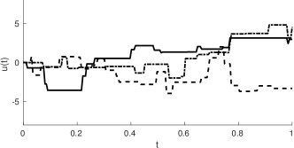
a)   b)

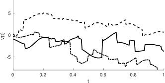
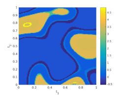
c)    d)

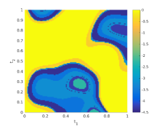
Fig. 3: (a) Three samples from the compound Poisson process (18) with normal jumps depicting the piecewise constant sample paths. (b) Samples from the $v(t)$ process generated using (21) by combining a smooth Gaussian process and an independent compound Poisson process with normal jumps. (c,d) Two draws from the random field $u(\mathbf{t})$ generated using (22) by combining a smooth Gaussian field with a Poisson process.

3.2 Extension to higher dimensions

At the end of this section we discuss some possibilities for extension of the compound Poisson process priors to random fields in $BV(\Omega)$ for compact domains $\Omega\subset\mathbb{R}^{n}$, for $n=2,3$, with Lipschitz boundary. Let $g$ be a Gaussian process on $\Omega$ with kernel $\kappa(r,s)=\exp(-|{r-s}|^{2})$ i.e.

$$(g({t}_{1}),\cdots,g({t}_{n}))^{T}\sim\mathcal{N}(0,\mathbf{K}),\quad\mathbf{K}_{k,j}=\kappa({t}_{k},{t}_{j})\quad\text{for any collection}\quad{t}_{1},\cdots{t}_{n}\in\Omega.$$

Under these assumptions $g\in C^{\infty}(\Omega)$ a.s. Now consider the random field

(22) $$u({t})=\sum_{k=1}^{\tau(g^{+}({t}))}\xi_{k},\qquad\text{for }t\in\Omega\qquad\text{where }g^{+}(t):=\max\{0,g(t)\}.$$

As before, $\tau$ is an independent Poisson random variable with rate $c>0$ and $\{\xi_{k}\}$ is a sequence of i.i.d. random variables distributed according to the probability measure $c^{-1}\lambda$. It is straightforward to check that samples from $u$ are piecewise constant functions on $\Omega$ that jump along a finite number of the positive level sets of the field $g$. These level sets are chosen by the poisson random variable $\tau$. Since we assumed that $g$ is in $C^{\infty}(\Omega)$ a.s. we expect that the level sets of $g$ are also smooth and so $u$ is a piecewise constant function that jumps along finitely many smooth curves (surfaces). We will now check whether the law of the field $u$ is indeed supported on $BV(\Omega)$.

In what follows we will occasionally suppress the dependence of different functions on $t$ to make the expressions more readable. Consider a test function $\phi\in C^{\infty}_{c}(\Omega;\mathbb{R}^{n})$ so that $|\phi(t)|\leq 1$. We can write

$$\int_{\Omega}u\>\text{div}\phi\>\text{d}\Lambda(t)=\int_{\Omega}\left(\sum_{k=1}^{\tau(g^{+})}\xi_{k}\right)\>\text{div}\phi\>\text{d}\Lambda(t)=\sum_{j=1}^{\tau(\max g^{+})}\int_{A_{j}}\left(\sum_{k=1}^{j}\xi_{k}\right)\>\text{div}\phi\>\text{d}\Lambda(t)$$

with the convention that the sum inside the integral is set to zero whenever $\tau(\max g^{+})=0$. The sets $A_{j}:=\{t\in\Omega\>\big{|}\>\tau(g^{+}(t))=j\}$ are the subsets of $\Omega$ on which $u$ is constant. Since $\tau$ is almost surely finite, we can integrate by parts [24, Thm. 5.6] to get

$$\int_{\Omega}u\>\text{div}\phi\>\text{d}\Lambda(t)=\sum_{j=1}^{\tau(\max g^{+})}\int_{\partial A_{j}}\mathcal{J}_{j}(u)\langle\phi,\vartheta_{j}\rangle\text{d}\Theta_{j}^{n-1}(s).$$

Here $\partial A_{j}$ is the boundary of $A_{j}$, $\vartheta_{j}$ is the unit outward normal on $\partial A_{j}$, $\mathcal{J}_{j}(u)$ is the jump of $u$ across $\partial A_{j}$ going from $A_{j-1}$ to $A_{j}$ and $\Theta_{j}^{n-1}$ are the $(n-1)$-dimensional Hausdorff measures on $\partial A_{j}$ [24, Ch. 2]. Recall that the $(n-1)$-dimensional Hausdorff measure of a simple curve in 2D (resp. surface in 3D) coincides with its length (resp. surface area) [24, Sec. 3.4]. Since the size of the jumps of $u$ are a.s. finite we can write

$$\int_{\Omega}u\>\text{div}\phi\>\text{d}\Lambda(t) \leq\left(\sum_{k=1}^{\tau(\max g^{+})}|\xi_{k}|\right)\left(\sum_{j=1}^{\tau(\max g^{+})}\int_{\partial A_{j}}\langle\phi,\vartheta_{j}\rangle\text{d}\Theta_{j}^{n-1}(s)\right)$$

$$\leq\left(\sum_{k=1}^{\tau(\max g^{+})}|\xi_{k}|\right)\sum_{j=1}^{\tau(\max g^{+})}\Theta_{j}^{n-1}({\partial A_{j}})$$

The main question now is whether or not $\Theta_{j}^{n-1}(\partial A_{j})$ are finite a.s. This is solely a property of the field $g$. We need a generalization of Rice’s formula in order to respond to this question.

Theorem 21 ([4, Thm. 6.8 and Prop. 6.12]).

Let $\Omega$ be a compact set in $\mathbb{R}^{n}$ with $n\geq 1$. Let $z:\Omega\mapsto\mathbb{R}$ be a Gaussian random field so that $z\in C^{2}(\Omega)$ a.s. and $\mathbf{Var}z(t)>0$ for all $t\in\Omega$. For a fixed constant $b\in\mathbb{R}$, $\mathbb{E\>}{\Theta}^{n-1}(\{t\in\Omega|z(t)=b\})<\infty$ if the pair $(z(t),\nabla z(t))$ have a joint density on $\Omega\times\mathbb{R}^{n}$ that is locally bounded.

It is well known [1, Thm. 2.2.2] that for $j\in\{1,\cdots,n\}$ the processes $g_{j}(t):=\frac{\partial g}{\partial t_{j}}(t)$ are themselves Gaussian processes with kernels $\kappa_{j}(r,s)=\frac{\partial^{2}}{\partial r_{j}\partial s_{j}}\kappa(r,s)$ whenever the second order partial derivative of the kernel exists. Using this fact it is straightforward to check that our choice of the field $g$ satisfies the assumptions of the above theorem. Therefore, $\Theta_{j}^{n-1}(\partial A_{j})$ are finite a.s. and we conclude that $V(u)<\infty$ a.s.

We show two samples from the random field of (22) on the box $[0,1]^{2}$ in Figure 3(c–d) with standard normal jumps. The choice of the field $g$ influences the shape of the discontinuity curves of $u$. The main difficulty in proving $u\in BV(\Omega)$ is in showing that the level sets of the underlying Gaussian field have finite length. Theorem 21 allows us to relax the regularity assumptions on $g$ and take Gaussian fields that are in $C^{2}(\Omega)$ rather than $C^{\infty}(\Omega)$ but for less regular fields it is not clear whether the level sets have finite length. Finally, one can show that the law of the process in (22) is a Radon measure on $BV(\Omega)$. The method of proof is identical to our argument for the 1D case except that now we need a different version of Helly’s selection principle [24, Thm. 5.5] in order to construct compact sets in $BV(\Omega)$.

4 Well-posed Bayesian inverse problems

Recall from Section 1 that we are interested in the problem of inferring a parameter $u\in X$ from data $y\in Y$ that are related via a generic stochastic mapping $\tilde{\mathcal{G}}$ that models the physical process that generates the data as well as the measurement noise:

$$y=\tilde{\mathcal{G}}(u).$$

In order to solve this problem we employ Bayes’ rule (2). In this section we collect certain conditions on the prior measure $\mu_{0}$ and the likelihood potential $\Phi$ that result in well-posed inverse problems. We consider a general enough setting that encompasses the heavy-tailed priors of Section 2 and the stochastic process priors of Section 3. We assume that the parameter space $X$ is a Banach space that is not necessarily separable (such as $BV$) and the prior measure $\mu_{0}$ is possibly heavy-tailed (such as the $G_{p,q}$-priors) and not necessarily Radon (such as the law of the pure jump Lévy processes when $\lambda$ is not finite).

The main results of this section are Theorems 23 and 24 that establish the existence, uniqueness and stability of the posterior measure. We acknowledge that these theorems are very similar to the results in [22, Sec. 4.1] and [52]. In comparison to these articles, we impose slightly different assumptions on the potential $\Phi$ and assume that the space $X$ is not necessarily separable. We also note that under the assumption that the prior measure $\mu_{0}$ is a Radon measure one can immediately generalize the result of [22] to non-separable parameter spaces $X$ using the fact that Radon measures on a Banach space are automatically concentrated on a separable subspace.

Theorem 22 ([9, Thm. 7.12.4]).

Let $\mu$ be a Radon probability measure on a Banach space $X$. Then, there exists a reflexive and separable Banach space $E$ embedded in $X$ such that $\mu(X\setminus E)=0$ and the closed balls of $E$ are compact in $X$.

It is important to note that while this theorem guarantees the existence of the separable space $E$ it does not provide us with a method for identifying $E$ or its norm. In the case of the product priors of Section 2 one can argue that the measures are concentrated on a separable Hilbert space but for the stochastic process priors of Section 3 it is no longer clear what the space $E$ is and so it is more convenient for us to analyze the inverse problem on the ambient space $X$ rather than passing to the space $E$.

We will present our well-posedness results using the total variation metric, since this metric is less often used in previous works, and refer the reader to [22] for proofs using the Hellinger metric that can easily be generalized to our setting by comparison to the proofs using the total variation metric. Given the inequalities (6) we immediately see that well-posedness in one of these metrics implies well-posedness in the other but the convergence rates will differ.

We start by presenting minimal assumptions on the likelihood potential and the forward map and make our way to more specific cases of inverse problems such as problems with linear forward maps. In a nutshell, as we put more restrictions on $\Phi$ we are able to relax our assumptions on $\mu_{0}$. In order to help with navigation through this section we present Table 1 that collects our main results and the key underlying assumptions.

Theorem/Corollary	Main assumptions	type of result
Theorem 23	$\Phi$ is locally bounded and Lipschitz in $u$.	$\mu^{y}$ is well-defined
Theorem 24	$\Phi$ satisfies Assumption 1	$\mu^{y}$ depends continuously on $y$
Corollary 25	$\Phi$ has polynomial growth in $u$ and $\mu_{0}$ has finitely many moments	well-posedness
Corollary 27	$\Phi\geq 0$ in addition to Assumption 1	well-posedness
Corollary 29	$Y=\mathbb{R}^{m}$, measurement noise is additive and Gaussian, prior is ID	well-posedness
Corollary 30	$Y=\mathbb{R}^{m}$, forward map is linear and bounded, measurement noise is additive and Gaussian	well-posedness
Corollary 32	$Y=\mathbb{R}^{m}$, forward map is linear and bounded, measurement noise is additive and Gaussian, $G_{p,q}$-prior	well-posedness

Table 1: Summary of the key theorems and corollaries of Section 4. In each case we identify the key underlying assumptions as well as the type of final result.

We begin by identifying some conditions on $\Phi$ that allow us to use a very large class of prior measures including those that are heavy-tailed.

Assumption 1.

Suppose that $X$ and $Y$ are Banach spaces and the likelihood potential $\Phi:X\times Y\mapsto\mathbb{R}$ satisfies the following properties:

1. (Lower bound in $u$): There is a positive and non-decreasing function $f_{1}:\mathbb{R}_{+}\mapsto[1,\infty)$ so that $\forall r>0$, there is a constant $M(r)\in\mathbb{R}$ such that,

   $$\Phi(u;y)\geq M(r)-\log\left(f_{1}(\|u\|_{X})\right),\qquad\forall u\in X\text{ and }\forall y\in B_{Y}(r).$$

2. (Boundedness above): $\forall r>0$ there is a constant $K(r)>0$ such that

   $$\Phi(u;y)\leq K(r),\qquad\forall u\in B_{X}(r)\text{ and }\forall y\in B_{Y}(r).$$

3. (Continuity in $u$): $\forall r>0$ there exists a constant $L(r)>0$ such that

   $$|\Phi(u_{1};y)-\Phi(u_{2},y)|\leq L(r)\|u_{1}-u_{2}\|_{X},\qquad\forall u_{1},u_{2}\in B_{X}(r)\text{ and }y\in B_{Y}(r).$$

4. (Continuity in $y$): There is a positive and non-decreasing function $f_{2}:\mathbb{R}_{+}\mapsto\mathbb{R}_{+}$ so that $\forall r>0$, there is a constant $C(r)\in\mathbb{R}$ such that

   $$|\Phi(u;y_{1})-\Phi(u,y_{2})|\leq C(r)f_{2}(\|u\|_{X})\|y_{1}-y_{2}\|_{Y},\qquad\forall y_{1},y_{2}\in B_{Y}(r)\text{ and }\forall u\in X.$$

Our first task is to establish the existence and uniqueness of the posterior measure.

Theorem 23.

Suppose $X$ is a Banach space, $\mu_{0}$ is a Borel probability measure on $X$ and let $\Phi$ satisfy Assumptions 1 (i), (ii) and (iii) with a function $f_{1}\geq 1$. If $f_{1}(\|\cdot\|_{X})\in L^{1}(X,\mu_{0})$ then the posterior $\mu^{y}$ given by (2) is a well-defined Borel probability measure on $X$. If $\mu_{0}$ is Radon then so is $\mu^{y}$.

Proof.

Our proof will closely follow the approach of [52, Thm. 4.3] and [34, Thm. 2.2]. Assumption 1(iii) implies the continuity of $\Phi$ on $X$ which in turn implies that $\Phi(\cdot,y):X\mapsto\mathbb{R}$ is $\mu_{0}$-measurable. We will now show that the normalizing constant satisfies $0<Z(y)<\infty$ which proves that $\mu^{y}$ is well-defined. The assertion that $\mu^{y}$ inherits the Radon property of $\mu_{0}$ will then follow from the absolute continuity of $\mu^{y}$ with respect to $\mu_{0}$ [9, Lem. 7.1.11].

Following Assumption 1(i) we can write

$$Z(y) \leq\int_{X}\exp(\log(f_{1}(\|u\|_{X}))-M)\text{d}\mu_{0}(u)=\exp(-M)\int_{X}f_{1}(\|u\|_{X})\text{d}\mu_{0}(u)<\infty.$$

We now need to show that the normalizing constant $Z(y)$ does not vanish. It follows from Assumption 1 that for $R>0$

$$Z(y) \geq\int_{B_{X}(R)}\exp(-K)\text{d}\mu_{0}(u)=\exp(-K)\mu_{0}(B_{X}(R)).$$

However, $\mu_{0}(B_{X}(R))>0$ for large enough $R$. To see this consider the disjoint sets $A_{k}:=\{u|k-1\leq\|u\|_{X}<k\}$ for $k\in\mathbb{N}$. The $A_{k}$ are open and hence measurable and $\sum_{k=1}^{\infty}\mu_{0}(A_{k})=\mu_{0}(\bigcup_{k=1}^{\infty}A_{k})=\mu(X)=1$. Then the measure of at least one of the $A_{k}$ has to be nonzero. ∎

We now establish the stability of Bayesian inverse problems with respect to perturbations in the data. Similar versions of the following theorems are available for Gaussian priors in [51], for Besov priors in [21], for convex priors in [34] and for heavy-tailed priors on separable Banach spaces in [22, 52].

Theorem 24.

Suppose that $X$ is a Banach space, $\mu_{0}$ is a Borel probability measure on $X$ and $\Phi$ satisfies Assumptions 1(i), (ii) and (iv) with functions $f_{1},f_{2}$. Let $\mu^{y}$ and $\mu^{y^{\prime}}$ be two measures defined via (2) for any $y$ and $y^{\prime}\in Y$, both absolutely continuous with respect to $\mu_{0}$.

1. If $f_{2}(\|\cdot\|_{X})f_{1}(\|\cdot\|_{X})\in L^{1}(X,\mu_{0})$ then $\forall r>0$, there exists a constant $C(r)>0$ so that $d_{TV}(\mu^{y},\mu^{y^{\prime}})\leq C\|y-y^{\prime}\|_{Y},\forall y,y^{\prime}\in B_{Y}(r)$

2. If instead $(f_{2}(\|\cdot\|_{X}))^{2}f_{1}(\|\cdot\|_{X})\in L^{1}(X,\mu_{0})$ then $\forall r>0$ there exists a constant $C^{\prime}(r)>0$ so that $d_{H}(\mu^{y},\mu^{y^{\prime}})\leq C^{\prime}\|y-y^{\prime}\|_{Y}.$

Proof.

We will only prove (i) and refer the reader to [22, Sec. 4.1] for the proof of (ii) that will readily generalize to our setting. Consider the normalizing constants $Z(y)$ and $Z(y^{\prime})$. We have already established in the proof of Theorem 23 that neither of these constants will vanish and they are both bounded. Thus the measures $\mu^{y}$ and $\mu^{y^{\prime}}$ are well-defined. Applying the mean value theorem to the exponential function and using Assumptions 1(i), (iv) and the assumption that $f_{2}(\|\cdot\|_{X})f_{1}(\|\cdot\|_{X})\in L^{1}(X,\mu_{0})$ we obtain

(23) $$|Z(y)-Z(y^{\prime})| \leq\int_{X}\exp(-\Phi(u;y))|\Phi(u;y)-\Phi(u;y^{\prime})|\text{d}\mu_{0}(u)$$

$$\leq\left(\int_{X}\exp(\log(f_{1}(\|u\|_{X}))-M)Cf_{2}(\|u\|_{X})\text{d}\mu_{0}(u)\right)\|y-y^{\prime}\|_{Y}$$

$$\leq C\exp(-M)\left(\int_{X}f_{1}(\|u\|_{X})f_{2}(\|u\|_{X})\text{d}\mu_{0}(u)\right)\|y-y^{\prime}\|_{Y}\lesssim\|y-y^{\prime}\|_{Y}.$$

Following the definition of the total variation distance we have

$$2d_{TV}(\mu^{y},\mu^{y^{\prime}}) =\int_{X}\left|Z(y)^{-1}\exp(-\Phi(u;y))-Z(y^{\prime})^{-1}\exp(-\Phi(u,y^{\prime}))\right|\text{d}\mu_{0}(u)$$

$$\leq\int_{X}\left|Z(y)^{-1}\exp(-\Phi(u;y))-Z(y^{\prime})^{-1}\exp(-\Phi(u,y))\right|\text{d}\mu_{0}(u)$$

$$\quad+Z(y^{\prime})^{-1}\int_{X}\left|\exp(-\Phi(u;y))-\exp(-\Phi(u,y^{\prime}))\right|\text{d}\mu_{0}(u)=:I_{1}+I_{2}.$$

Now using (23) we have

$$I_{1}=|Z(y)^{-1}-Z(y^{\prime})^{-1}|Z(y)=\frac{Z(y)}{Z(y^{\prime})}|Z(y^{\prime})-Z(y)|\lesssim\|y-y^{\prime}\|_{X}.$$

Furthermore, using the mean value theorem, Assumption 1 (i) and (iv) we can write

$${Z(y^{\prime})}{I_{2}} =\int_{X}\left|\exp(-\Phi(u;y))-\exp(-\Phi(u,y^{\prime}))\right|\text{d}\mu_{0}(u)$$

$$\leq\int_{X}\exp(-\Phi(u;y))\left|\Phi(u;y^{\prime})-\Phi(u,y)\right|\text{d}\mu_{0}(u)$$

$$\leq C\exp(-M)\left(\int_{X}\exp(\log(f_{1}(\|u\|_{X})))f_{2}(\|u\|_{X})\text{d}\mu_{0}(u)\right)\|y-y^{\prime}\|_{Y}\lesssim\|y-y^{\prime}\|_{Y}.$$

∎

The main distinction between the choice of the metrics in Theorem 24 is that in order to obtain the same rate of convergence in the Hellinger metric we need a (possibly) stronger assumption regarding the integrability of $f_{1}(\|u\|_{X})$ and $f_{2}(\|u\|_{X})$. So far we encountered conditions of the form $(f_{2}(\|u\|_{X}))^{p}f_{1}(\|u\|_{X})\in L^{1}(X,\mu_{0})$ for $p\in\{0,1,2\}$. Intuitively, these conditions identify the interplay between the growth of $\Phi(u;y)$ as a function of $\|u\|_{X}$ and the tail behavior of the prior $\mu_{0}$.

Corollary 25.

Suppose that $\Phi$ satisfies the conditions of Assumption 1 with $f_{1}(t)=f_{2}(t)=\max\{1,|t|^{p}\}$ for $p\geq 0$ and $\mu_{0}$ is a Borel probability measure on $X$. If $\mu_{0}$ has bounded raw moments of degree up to $\lceil 2p\rceil$ then the Bayesian inverse problem (2) is well-posed in both the total variation and Hellinger metrics.

Corollary 26.

Suppose that $\mu_{0}$ is a Borel probability measure on $X$ and $\exp(b\|\cdot\|_{X})\in L^{1}(X,\mu_{0})$ for some constant $b>0$. Then the Bayesian inverse problem (2) is well-posed in both the total variation and Hellinger metrics whenever $\Phi$ satisfies the conditions of Assumption 1 with functions $f_{1},f_{2}$ that are polynomially bounded.

For the remainder of this section we will focus on specific classes of likelihood potentials $\Phi$ which allow us to further relax our assumption regarding the tail behavior of $\mu_{0}$. The rest of our results follow from Theorems 23 and 24 but they are of great interest in practical applications. We start with the case of additive noise models and consider linear inverse problems afterwards.

4.1 The case of additive noise models

Additive noise models have a special place in practical applications due to their convenience and flexibility [36]. Suppose that the data is finite dimensional and, without loss of generality, take $Y=\mathbb{R}^{m}$, $m\in\mathbb{N}$. Now suppose that $y\in Y$ is related to the parameter $u\in X$ via the model

(24) $$y=\mathcal{G}(u)+\eta\qquad\eta\sim\pi(y)\text{d}\Lambda(y)$$

where $\pi(y)$ is the Lebesgue density of the measurement noise $\eta$ and $\mathcal{G}:X\mapsto\mathbb{R}^{m}$ is the forward map. It is straightforward to check that under these assumptions

(25) $$\Phi(u;y)=-\log\pi(\mathcal{G}(u)-y).$$

In particular if $\eta\sim\mathcal{N}(0,\boldsymbol{\Sigma})$ with an $m\times m$ positive definite matrix $\boldsymbol{\Sigma}$ then

(26) $$\Phi(u;y)=\frac{1}{2}\left\|(\mathcal{G}(u)-y)\right\|_{\boldsymbol{\Sigma}}^{2}.$$

Now if $\log\pi(y)\leq 0$ (which is clearly the case when $\eta$ is Gaussian or Laplace) then $\Phi(u;y)$ will satisfy Assumption 1(i) with the constant $M=0$ and $f_{1}(x)=1$. This observation will allow us to relax our assumption on the tail behavior of the prior whenever the measurement noise is additive.

Corollary 27.

Suppose $Y=\mathbb{R}^{m}$, $X$ is a Banach space and $\Phi(u;y)\geq 0$ and it satisfies Assumptions (ii) and (iv) with a function $f_{2}$. Suppose that the prior measure $\mu_{0}$ is a Borel probability measure on $X$ and let $\mu^{y}$ and $\mu^{y^{\prime}}$ be two measures defined via (2) for $y$ and $y^{\prime}\in Y$. Then the posterior measure $\mu^{y}$ is well-defined and

1. If $f_{2}(\|\cdot\|_{X})\in L^{1}(X,\mu_{0})$ then $\forall r>0,\exists C(r)>0$ so that $d_{TV}(\mu^{y},\mu^{y^{\prime}})\leq C(r)\|y-y^{\prime}\|_{Y}\text{ for all }y,y^{\prime}\in B_{Y}(r).$

2. If $f_{2}(\|\cdot\|_{X})\in L^{2}(X,\mu_{0})$ then $\exists C^{\prime}(r)>0$ $d_{H}(\mu^{y},\mu^{y^{\prime}})\leq C^{\prime}(r)\|y-y^{\prime}\|_{Y}.$

At this point it is natural to identify conditions on the distribution of the noise and the forward operator that guarantee that the likelihood potential of (25) satisfies the conditions of Assumption 1. We will address this when $\eta$ is Gaussian but our approach can be generalized to other types of additive noise models.

Theorem 28.

Consider the additive noise model of (24) when $\eta\sim\mathcal{N}(0,\boldsymbol{\Sigma})$ and $\boldsymbol{\Sigma}$ is a positive-definite matrix. Then the corresponding likelihood potential $\Phi(u;y)\geq 0$. Furthermore, $\Phi$ satisfies the conditions of Assumption 1(iv) with $f_{2}(x)=1+\tilde{f}(x)$ if there is a positive, non-decreasing and locally bounded function $\tilde{f}:\mathbb{R}_{+}\mapsto\mathbb{R}_{+}$ so that

1. $\exists C>0$ for which $\|\mathcal{G}(u)\|_{2}\leq C\tilde{f}(\|u\|_{X}),\forall u\in X.$

2. $\forall r>0,\exists K(r)>0$ so that $\|\mathcal{G}(u_{1})-\mathcal{G}(u_{2})\|_{2}\leq K(r)\|u_{1}-u_{2}\|_{X}$ for all $u_{1},u_{2}\in B_{X}(r)$.

Proof.

Since we assumed that $\eta$ is Gaussian then the likelihood potential is of the form (26). Then it is clear that $\Phi(u;y)\geq 0$ which immediately implies that $\Phi$ satisfies Assumption 1(i) with $M=0$ and $f_{1}(x)=0$. Now fix $r>0$ and suppose that $u\in B_{X}(r)$ and $y\in B_{Y}(r)$. Define $\tilde{r}=\max\{r,C\tilde{f}(r)\}$ and note that $\tilde{r}$ is bounded since we assumed that $\tilde{f}$ is locally bounded. Therefore, we have $\Phi(u;y)\leq\|\mathcal{G}(u)\|_{\boldsymbol{\Sigma}}^{2}+\|y\|_{\boldsymbol{\Sigma}}^{2}\lesssim\tilde{r}^{2}$ and so $\Phi$ satisfies Assumption 1(ii).

Now we will show that $\Phi$ satisfies Assumption 1(iii) as well. Let $r$ and $\tilde{r}$ be defined as above and consider $u_{1},u_{2}\in B_{X}(r)$ and $y\in B_{Y}(r)$. Using the identity $\|a\|_{2}^{2}-\|b\|_{2}^{2}=\langle a-b,a+b\rangle$ for $a,b\in\mathbb{R}^{m}$ and the conditions (i) and (ii) of the theorem we obtain

$$2|\Phi(u_{1};y)-\Phi(u_{2};y)| =\left|\langle\boldsymbol{\Sigma}^{-1/2}(\mathcal{G}(u_{1})-\mathcal{G}(u_{2})),\boldsymbol{\Sigma}^{-1/2}(\mathcal{G}(u_{1})+\mathcal{G}(u_{2})-2y)\rangle\right|$$

$$\leq\left(\|\mathcal{G}(u_{1})\|_{\boldsymbol{\Sigma}}+\|\mathcal{G}(u_{2})\|_{\boldsymbol{\Sigma}}+2\|y\|^{2}_{\boldsymbol{\Sigma}}\right)\|(\mathcal{G}(u_{1})-\mathcal{G}(u_{2}))\|_{\boldsymbol{\Sigma}}$$

$$\leq C(\tilde{r})\|(\mathcal{G}(u_{1})-\mathcal{G}(u_{2}))\|_{\boldsymbol{\Sigma}}\leq 2K(r)\|u_{1}-u_{2}\|_{X}.$$

Finally, fix $r>0$ and consider $y_{1},y_{2}\in B_{Y}(r)$. Then using the same line of reasoning as above, for any $u\in X$ we can write

$$2|\Phi(u;y_{1})-\Phi(u;y_{2})| =\left|\langle\boldsymbol{\Sigma}^{-1/2}(y_{2}-y_{1}),\boldsymbol{\Sigma}^{-1/2}(2\mathcal{G}(u)-y_{1}-y_{2})\rangle\right|$$

$$\leq\left(\|y_{2}\|_{\boldsymbol{\Sigma}}-\|y_{1}\|_{\boldsymbol{\Sigma}}+2\|\mathcal{G}(u)\|_{\boldsymbol{\Sigma}}\right)\|(y_{2}-y_{1})\|_{\boldsymbol{\Sigma}}$$

$$\leq C(r)(1+\tilde{f}(\|u\|_{X}))\|y_{1}-y_{2}\|_{2}.$$

∎

By putting this result together with Theorem 16 and Corollary 27 we deduce the following corollary concerning the well-posedness of Bayesian inverse problems with ID priors.

Corollary 29.

Let $X$ be a Banach space and $Y=\mathbb{R}^{m}$. Consider the additive noise model:

$$y=\mathcal{G}(u)+\eta,\qquad\eta\sim\mathcal{N}(0,\boldsymbol{\Sigma})$$

where $\boldsymbol{\Sigma}$ is a positive definite matrix and $\mathcal{G}:X\mapsto\mathbb{R}^{m}$ satisfies the conditions of Theorem 28 with a submultiplicative function $\tilde{f}$. Also, suppose that $\mu_{0}=\text{ID}(m,\mathcal{R},\lambda)$ where $\lambda$ is a Lévy measure such that $\lambda(X)<\infty$, $\mu_{0}(X)=1$ and $\|\cdot\|_{X}<\infty$ $\mu_{0}$-a.s. Then the Bayesian inverse problem (2) is well-posed if $1+\tilde{f}(\|\cdot\|_{X})\in L^{1}(X,\lambda)$.

4.2 The case of linear inverse problems

We now assume that the likelihood potential $\Phi$ has the form

$$\Phi(u;y):X\times\mathbb{R}^{m}\mapsto\mathbb{R},\qquad\Phi(u;y)=\frac{1}{2}\left\|\mathcal{G}(u)-y\right\|_{\boldsymbol{\Sigma}}^{2}$$

where $\boldsymbol{\Sigma}$ is a positive definite matrix and $\mathcal{G}:X\mapsto\mathbb{R}^{m}$ is bounded and linear. This case is of particular importance due to its occurrence in the Compressed Sensing literature [26] and estimation of sparse parameters. In this case, we can further relax our conditions on the prior measure $\mu_{0}$ and achieve well-posedness so long as the prior $\mu_{0}$ has bounded first moment.

Corollary 30.

Let $X$ be a Banach space and $Y=\mathbb{R}^{m}$. Suppose that the forward map $\mathcal{G}:X\mapsto\mathbb{R}^{m}$ is bounded and linear and consider the additive noise model

$$y=\mathcal{G}(u)+\eta\qquad where\qquad\eta\sim\mathcal{N}(0,\boldsymbol{\Sigma})\qquad\text{and}\qquad\text{$\boldsymbol{\Sigma}$ is positive definite}.$$

Then the Bayesian inverse problem of identifying the posterior $\mu^{y}$ via (2) is well-posed in both the Hellinger and total variation metrics if the prior $\mu_{0}$ is a Borel probability measure on $X$ and $\|\cdot\|_{X}\in L^{1}(X,\mu_{0})$.

Proof.

Follows directly from Theorems 28 and 23 and Corollary 27(i). ∎

Let us now return to the product priors of Section 2.1 and show that those measures result in well-posed Bayesian inverse problems under the linear and additive noise assumptions.

Theorem 31.

Let $X$ be a Banach space with an unconditional Schauder basis $\{x_{k}\}$ and take $Y=\mathbb{R}^{m}$. Suppose that the measurement noise is additive and Gaussian and the forward map $\mathcal{G}$ is bounded and linear. Furthermore, suppose that $\mu_{0}$ is a product prior with sample paths $u=\sum_{k=1}^{\infty}\gamma_{k}\xi_{k}x_{k}$ where $\{\gamma_{k}\}\in\ell^{2}$ and $\{\xi_{k}\}$ are i.i.d. and $\mathbf{Var}\xi_{k}<\infty$. Then the inverse problem (2) is well-posed in both the total variation and Hellinger metrics.

Proof.

The fact that $\mu_{0}$ is a Radon probability measures on $X$ follows from Theorem 3 and Theorem 2. Now if $\mathbf{Var}\xi_{k}<\infty$ then $\mathbb{E\>}\xi_{k}^{2}<\infty$ as well and so it follows from Theorem 4 that $\|\cdot\|_{X}\in L^{2}(X,\mu)$. Then the assertion follows from Theorems 27 and 28. ∎

Finally we turn our attention to the the $G_{p,q}$-priors of Section 2. The proof of the following corollary follows directly from Theorem 4 and the fact that the $G_{p,q}$ distributions in 1D have bounded variance for $0<p,q\leq 1$.

Corollary 32.

Let $X$ be a Banach space with an unconditional Schauder basis $\{x_{k}\}$ and $Y=\mathbb{R}^{m}$. Suppose that the measurement noise is additive and Gaussian and that the forward map $\mathcal{G}$ is bounded and linear. Then the Bayesian inverse problem (2) is well-posed in both the Hellinger and total variation metrics if $\mu_{0}$ is an $G_{p,q}$-prior with $0<p,q<1$.

5 Practical considerations and examples

We now turn our attention to practical aspects of solving an inverse problem within the Bayesian framework. In the first part of this section we discuss the problem of approximating the posterior measure via approximation of the likelihood potential. Afterwards, we will present three concrete examples of Bayesian inverse problems with heavy-tailed priors that arise from practical problems in image deblurring and ultrasound therapy.

5.1 Consistent approximation of the posterior

Up to this point we were concerned with identifying prior measures $\mu_{0}$ that result in a well-posed Bayesian inverse problem for a given likelihood potential $\Phi$. However, in practice we cannot solve the inverse problem directly on the infinite-dimensional Banach space. Therefore, we need to obtain a finite dimensional approximation to the posterior measure $\mu^{y}$ which is, in some sense, consistent with the infinite dimensional limit.

To this end, we will define the notion of consistent approximation of a Bayesian inverse problem in the context of applications where one would discretize (2) by approximating the likelihood potential $\Phi$ with a discretized version $\Phi_{N}:X\times Y\mapsto\mathbb{R}$, akin to a finite element discretization. We define the approximation $\mu^{y}_{N}$ to $\mu^{y}$ via

(27) $$\frac{\text{d}\mu^{y}_{N}}{\text{d}\mu_{0}}=\frac{1}{Z_{N}(y)}\exp(-\Phi_{N}(u;y))\qquad\text{where}\qquad Z_{N}(y)=\int_{X}\exp(-\Phi_{N}(u;y))\text{d}\mu_{0}(u).$$

Definition 33 (Consistent approximation[34]).

The approximate Bayesian inverse problem (27) is a consistent approximation to (2) for a choice of $\mu_{0}$, $\Phi$ and $\Phi_{N}$ if $d(\mu^{y},\mu^{y}_{N})\mapsto 0$ as $|\Phi(u;y)-\Phi_{N}(u;y)|\mapsto 0$. Here, $d$ is either the total variation or the Hellinger metric.

This notion of a consistent approximation relates directly to practical applications. Suppose, for example, that we are interested in computing the expected value of a quantity $h(u)$ under the posterior $\mu^{y}$ but we can only compute the expectation under the approximation $\mu^{y}_{N}$. If $\mu^{y}_{N}$ is a consistent approximation in the Hellinger metric then we have, by the bound (7), that if $h\in L^{2}(X,\mu^{y})\cap L^{2}(X,\mu^{y}_{N})$ then

$$\left|\int_{X}h(u)\text{d}\mu^{y}(u)-\int_{X}h(u)\text{d}\mu^{y}_{N}(u)\right|\leq Cd_{H}(\mu^{y},\mu^{y}_{N}).$$

In what follows, we will provide sharper bounds on the rate of convergence of the distances between $\mu^{y}$ and $\mu^{y}_{N}$ under mild conditions.

Theorem 34.

Assume that the measures $\mu^{y}$ and $\mu^{y}_{N}$ are defined via (2) and (27), for a fixed $y\in Y$ and all values of $N$, and are absolutely continuous with respect to the prior $\mu_{0}$ which is a Borel probability measure on $X$. Also assume that both $\Phi$ and $\Phi_{N}$ satisfy Assumptions 1(i) and (ii) with an appropriate function $f_{1}$, uniformly for all $N$ and that there exists a positive and non-decreasing function $f_{3}:\mathbb{R}_{+}\mapsto\mathbb{R}_{+}$ so that

(28) $$|\Phi(u;y)-\Phi_{N}(u;y)|\leq f_{3}(\|u\|_{X})\rho(N)$$

where $\rho(N)\mapsto 0$ as $N\mapsto\infty$.

1. If $f_{3}(\|\cdot\|_{X})f_{1}(\|\cdot\|_{X})\in L^{1}(X,\mu_{0})$ then there exists a constant $D>0$, independent of $N$ such that $d_{\text{TV}}(\mu^{y},\mu^{y}_{N})\leq D\rho(N).$

2. If $(f_{3}(\|\cdot\|_{X}))^{2}f_{1}(\|\cdot\|_{X})\in L^{1}(X,\mu_{0})$ then there exists a constant $D^{\prime}>0$, independent of $N$ such that $d_{H}(\mu^{y},\mu^{y}_{N})\leq D^{\prime}\rho(N).$

Proof.

Our method of proof uses similar arguments as in Theorem 24 and so we will only present it briefly for the total variation distance. Proof of part (ii) can also be found in [22] for separable Banach spaces. The existence and uniqueness of the measures $\mu^{y}$ and $\mu^{y}_{N}$ follows from Theorem 23 for all values of $N$. Next, the mean value theorem, Assumption 1(i), (28) and the assumption that $f_{3}(\|\cdot\|_{X})f_{1}(\|\cdot\|_{X})$ is $\mu_{0}$-integrable give

$$|Z(y)-Z_{N}(y)| \leq\int_{X}\exp(-\Phi(u;y))|\Phi(u;y)-\Phi_{N}(u;y)|\text{d}\mu_{0}(u)$$

$$\leq\left(\int_{X}\exp(\log(f_{1}(\|u\|_{X}))-M)Cf_{3}(\|u\|_{X})\text{d}\mu_{0}(u)\right)\rho(N)\lesssim\rho(N).$$

Furthermore, we have

$$2d_{TV}(\mu^{y},\mu^{y^{\prime}}) \leq\int_{X}\left|Z(y)^{-1}\exp(-\Phi(u;y))-Z_{N}(y)^{-1}\exp(-\Phi(u,y))\right|\text{d}\mu_{0}(u)$$

$$\quad+Z_{N}(y)^{-1}\int_{X}\left|\exp(-\Phi(u;y))-\exp(-\Phi_{N}(u,y))\right|\text{d}\mu_{0}(u)=:I_{1}+I_{2}.$$

It then follows in a similar manner to proof of Theorem 24 that $I_{1}\lesssim\rho(N)$ and $I_{2}\lesssim\rho(N)$ which gives the desired result. ∎

We now consider a more specific setting where the prior measure $\mu_{0}$ has a product structure. Suppose that the likelihood potential $\Phi$ satisfies the Assumption 1 with some functions $f_{1},f_{2}$. Also, assume that the space $X$ has an unconditional Schauder basis $\{x_{k}\}$ and consider the sequence of spaces $(X_{N},\|\cdot\|_{X})$ where $X_{N}=\text{span}\{x_{k}\}_{k=1}^{N}$. These are linear subspaces of $X$ and for each $N\in\mathbb{N}$ we have $X=X_{N}\oplus X_{N}^{\bot}$, meaning that every $u\in X$ can be written as $u=u_{N}+u_{N}^{\bot}$ where $u_{N}\in X_{N}$ and $u_{N}^{\bot}\in X_{N}^{\bot}$.

Suppose that the prior measure $\mu_{0}$ has the product structure of (8) and assume that it has sufficiently fast decaying tails so that the posterior measure $\mu^{y}$ is well-defined. Observe that for every value of $N$ the product prior can be factored as

(29) $$\mu_{0}=\mu_{N}\otimes\mu_{N}^{\bot}$$

where $\mu_{N}$ and $\mu_{N}^{\bot}$ are Radon measures on $X_{N}$ and $X_{N}^{\bot}$. It is natural for us to discretize the potential $\Phi$ using a projection operator:

(30) $$\Phi_{N}(u;y):=\Phi(P_{N}u;y)$$

where $P_{N}:X\mapsto X_{N}$ is defined by $P_{N}(u)=u_{N}$. Next, define the approximate posterior measures $\mu^{y}_{N}$ as in (27) using the above definition of $\Phi_{N}$. Under these assumptions, the $\mu^{y}_{N}$ will factor as (see [34, Sec. 4.1] for the details)

(31) $$\mu^{y}_{N}=\nu_{N}\otimes\mu_{N}^{\bot},$$

where

$$\frac{\text{d}\nu_{N}}{\text{d}\mu_{N}}=\frac{1}{Z_{N}(y)}\exp(-\Phi(P_{N}u;y)).$$

In other words, the likelihood potential is only informative on the subspace $X_{N}$ and so by comparing (29) and (31) we see that the approximate posterior $\mu^{y}_{N}$ differs from the prior only on this subspace and it is identical to the prior on $X_{N}^{\bot}$. As an example, we now check whether this method for discretization of the posterior results in a consistent approximation to $\mu^{y}$ in the additive Gaussian noise case.

Theorem 35.

Consider the above setting where the posterior and the prior have the prescribed product structures and the $X_{N}$ are linear subpaces of $X$. Suppose that $\Phi$and $\Phi_{N}$ are given by

$$\Phi(u;y)=\frac{1}{2}\|\mathcal{G}(u)-y\|_{2}^{2},\qquad\Phi_{N}(u;y)=\frac{1}{2}\|\mathcal{G}(P_{N}u)-y\|_{2}^{2}$$

where $P_{N}:X\mapsto X_{N}$ is the projection operator that was defined before. Assume that the following conditions are satisfied:

1. $\|u-P_{N}u\|_{X}\leq\|u\|_{X}\rho(N).$

2. $\|\mathcal{G}(u)\|_{2}\leq C\tilde{f}_{1}(\|u\|_{X})\qquad\forall u\in X.$

3. $\|\mathcal{G}(u_{1})-\mathcal{G}(u_{2})\|_{2}\leq\tilde{f}_{2}(\max\{(\|u_{1}\|_{X},\|u_{2}\|_{X}\})\|u_{1}-u_{2}\|_{X}\qquad\forall u_{1},u_{2}\in X.$

Here $\rho$ is a positive function such that $\rho(N)\mapsto 0$ as $N\mapsto\infty$ and the functions $\tilde{f}_{1},\tilde{f}_{2}:\mathbb{R}_{+}\mapsto\mathbb{R}_{+}$ are non-decreasing and locally bounded and $\tilde{f}_{1}\geq 1$. Then

1. If $\tilde{f}_{1}(\|\cdot\|_{X})\tilde{f}_{2}(\|\cdot\|_{X})\in L^{1}(X,\mu_{0})$ then $\exists D>0$ independent of $N$ so that $d_{TV}(\mu^{y},\mu^{y}_{N})\leq D\rho(N).$

2. If $\tilde{f}_{1}(\|\cdot\|_{X})\tilde{f}_{2}(\|\cdot\|_{X})\in L^{2}(X,\mu_{0})$ then $\exists D^{\prime}>0$ independent of $N$ so that $d_{H}(\mu^{y},\mu^{y}_{N})\leq D^{\prime}\rho(N).$

Proof.

It follows from Theorem 28 that $\Phi$ and $\Phi_{N}$ satisfy Assumption 1 uniformly in $N$ with $M=0$, $f_{1}(x)=1$. Then the measures $\mu^{y}$ and $\mu^{y}_{N}$ are well-defined for all values of $N\in\mathbb{N}$ by Theorem 23. Now it follows from our assumptions on $\mathcal{G}$ that

$$2|\Phi(u;y)-\Phi_{N}(u;y)| =\left|\|(\mathcal{G}(u)-y)\|_{\boldsymbol{\Sigma}}^{2}-\|(\mathcal{G}(P_{N}u)-y)\|_{\boldsymbol{\Sigma}}^{2}\right|$$

$$=\left|\langle\boldsymbol{\Sigma}^{-1/2}(\mathcal{G}(u)-\mathcal{G}(P_{N}u)),\boldsymbol{\Sigma}^{-1/2}(\mathcal{G}(u)+\mathcal{G}(P_{N}u)-2y)\rangle\right|$$

$$\leq\left(\|\mathcal{G}(u)\|_{\boldsymbol{\Sigma}}+\|\mathcal{G}(P_{N}u)\|_{\boldsymbol{\Sigma}}+2\|y\|^{2}_{\boldsymbol{\Sigma}}\right)\|(\mathcal{G}(u)-\mathcal{G}(P_{N}u))\|_{\boldsymbol{\Sigma}}$$

$$\leq C\tilde{f}_{1}(\|u\|_{X})\tilde{f}_{2}(\|u\|_{X})\|u-P_{N}u\|_{X}.$$

The claim will now follow by taking $f_{3}(x)=\tilde{f}_{1}(x)\tilde{f}_{2}(x)$ and applying Theorem 34. ∎

A few comments are in order concerning the previous theorem. First, the function $\rho(N)$ is independent of the forward map and the prior and depends solely on the topology of $X$. Then the rate of convergence of $\mu^{y}_{N}$ to $\mu^{y}$ depends directly on the rate of convergence of $P_{N}$ to the identity map in the operator norm. Also, observe that in order to achieve the same rate of convergence in the Hellinger metric as in the total variation metric, we need to impose stronger tail assumptions on the prior $\mu_{0}$.

5.2 Example 2: Deconvolution

We now turn our attention to a few concrete examples of inverse problems with heavy-tailed or non-Gaussian prior measures. We begin with a problem in deconvolution which is a classic example of a linear inverse problem with wide applications in optics and imaging [57, 30]. This problem was also considered in [34] as an example problem with a convex prior measure.

Let $X=L^{2}(\mathbb{T})$ where $\mathbb{T}$ is the circle of radius $(2\pi)^{-1}$ and let $Y=\mathbb{R}^{m}$ for a fixed integer $m$. Suppose that $\eta\sim\mathcal{N}(0,\sigma^{2}\mathbf{I})$ where $\sigma\in\mathbb{R}$ is a fixed constant and $\mathbf{I}$ is the $m\times m$ identity matrix. Let $S:C(\mathbb{T})\mapsto\mathbb{R}^{m}$ be a bounded linear operator that collects point values of a continuous function on a set of $m$ points over $\mathbb{T}$. Given a fixed kernel $\varphi\in C^{1}(\mathbb{T})$, define the forward map $\mathcal{G}:X\rightarrow Y$ as

(32) $$\mathcal{G}(u)=S(\varphi\ast u)\qquad\text{where}\qquad(\varphi\ast u)(t):=\int_{\mathbb{T}}\varphi(t-s)u(t)d\Lambda(s).$$

Now suppose that the data $y$ is generated via $y=\mathcal{G}(u)+\eta$ and our goal is to estimate the original image $u$ given noisy point values of its blurred version. Note that our assumptions so far imply a quadratic likelihood potential of the form (26)

It follows from Young’s inequality [32, Thm. 13.8] that $(\varphi\ast\cdot):L^{2}(\mathbb{T})\mapsto L^{2}(\mathbb{T})$ is a bounded linear operator and furthermore, $(\varphi\ast u)\in C^{1}(\mathbb{T})$ for all $u\in L^{2}(\mathbb{T})$. Since pointwise evaluation is a bounded linear functional on $C^{1}(\mathbb{T})$ then the forward map $\mathcal{G}:L^{2}(\mathbb{T})\mapsto\mathbb{R}^{m}$ is bounded and linear. We will use the results of Section 4.2 to show this problem is well-posed.

We will take our prior measure to be in class of the product priors of Section 2.1. Consider the functions

$$\tilde{w}(t)=\left\{\begin{aligned} &1\quad 0\leq t\leq 1,\\ &0\quad\text{otherwise}.\end{aligned}\right.\qquad\text{and}\qquad\tilde{v}(t)=\left\{\begin{aligned} &1\quad 0\leq t\leq 1/2,\\ &1\quad 1/2\leq t\leq 1,\\ &0\quad\text{otherwise}.\end{aligned}\right.$$

The function $\tilde{v}$ is the Haar wavelet and $\tilde{w}$ is its corresponding scaling function. Following [23, Sec. 9.3], we can define the periodic functions

$$w_{jn}(t):=\sum_{l\in\mathbb{Z}}\phi(2^{j}(t+l)-n),\qquad v_{jn}(t):=\sum_{l\in\mathbb{Z}}\psi(2^{j}(t+l)-n),$$

as well as the functions

$$x_{1}(t)=w_{0,0}(t),\quad x_{2}(t)=v_{0,0}(t),\quad x_{2^{j}+n_{j}+1}(t)=v_{j,n_{j}}(t).$$

for $j\in\mathbb{Z}_{+}$ and $n_{j}=\{0,1,\cdots,2^{j}-1\}$. The $\{x_{k}\}$ form an orthonormal basis for $L^{2}(\mathbb{T})$ and so they can be used in the construction of a $G_{p,q}$-prior.

Now choose $p,q\in(0,1)$ and take the prior $\mu_{0}$ to be the $G_{p,q}$-prior generated by the wavelet basis $\{x_{k}\}$ and the fixed sequence $\{\gamma_{k}\}$ where

$$\gamma_{2^{j}+n+1}=(1+|2^{j+1}|^{2})^{-1/2}\qquad\forall n\in\mathbb{Z}_{+}.$$

Clearly, $\{\gamma_{k}\}\in\ell^{2}$ and so it follows from Theorem 2 that $\|u\|_{L^{2}(\mathbb{T})}<\infty$ a.s. Furthermore, we know that the $G_{p,q}$-priors have bounded moments of order two. Putting this together with the fact that the forward map $\mathcal{G}$ is bounded and linear we immediately obtain the well-posedness of this inverse problem using Theorem 31.

5.3 Example 3: Deconvolution with a BV prior

We now formulate the deconvolution problem of Example 2 with a prior measure that is supported on $BV(\mathbb{T})$ using the stochastic process priors of Section 3. Let $u(t)$ for $t\in[0,1]$ denote a stochastic process such that

$$u(0)=0,\qquad\hat{u}_{t}(s)\exp\left(t\int_{\mathbb{R}}\exp(i\xi s)-1\>\text{d}\nu(\xi)\right)\qquad s\in\mathbb{R}.$$

where the measure $\nu=c\mathcal{N}(0,1)$ with a fixed constant $c\in(0,\infty)$. Then $u$ is a compound Poisson process with piecewise constant sample paths and normal jumps. We can write $u(t)=\sum_{k=1}^{\tau(t)}\xi_{k},$ where $\{\xi_{k}\}$ is an i.i.d. sequence of standard normal random variables and $\tau(t)$ is a Poisson process with intensity $c$. In Section 3 we saw that this process has piecewise constant sample paths and its law is a Radon measure on $BV([0,1])$.

Let us denote the law of this process by $\tilde{\mu}_{0}$. The next step is to use this measure to define a new measure $\mu_{0}$ on $BV(\mathbb{T})$. Take $\mu_{0}$ to be the law of the periodic versions of the sample paths of the above compound Poisson process $u$ on the interval $[0,1]$. We can write $\mu_{0}=\tilde{\mu}_{0}\circ T^{-1}$ where $T:BV([0,1])\mapsto BV(\mathbb{T})$ is a bounded and linear operator. Thus, $\mu_{0}$ is a Radon measure on $BV(\mathbb{T})$. With an abuse of notation we use $u$ to denote the corresponding periodic processes on $\mathbb{T}$. Since the convolution kernel $\varphi\in C^{1}(\mathbb{T})$ and $BV(\mathbb{T})\subset L^{1}(\mathbb{T})$ then the forward map $\mathcal{G}:BV(\mathbb{T})\mapsto\mathbb{R}^{m}$ (given by(32)) is well-defined, bounded and linear and so the likelihood potential has the form (26) once more. We have shown, in Section 3 that $\mathbb{E\>}\|u\|_{BV(\mathbb{T})}<\infty$. Putting this together with the fact that $\mathcal{G}:BV(\mathbb{T})\mapsto\mathbb{R}^{m}$ is bounded and linear we immediately obtain the well-posedness of this inverse problem via Corollary 30.

5.4 Example 4: Quadratic measurements of a continuous field

As our final example, we will consider a problem with a non-linear forward map. Our goal is to estimate a continuous field from quadratic measurements of its point values. This inverse problem was encountered in [33] in recovery of aberrations in high intensity focused ultrasound treatment and it is closely related to the phase retrieval problem [25, 31, 15]. Let $X=C(\mathbb{T})$ and let $\{t_{k}\}_{k=1}^{n}$ be a collection of distinct points in $\mathbb{T}$. Now define the operator

$$S:C(\mathbb{T})\mapsto\mathbb{R}^{n}\qquad(S(u))_{j}=u(t_{j})\qquad j=1,2,\cdots,n.$$

This operator collects point values of functions in $C(\mathbb{T})$. Let $\{z_{k}\}_{k=1}^{m}$ be a fixed collection of vectors $z_{k}\in\mathbb{R}^{n}$ and define the forward map

$$\mathcal{G}:C(\mathbb{T})\mapsto\mathbb{R}^{m},\qquad(\mathcal{G}(u))_{j}:=|z_{j}^{T}S(u)|^{2}\qquad\text{for}\qquad j=1,2,\cdots,m,$$

which collects quadratic measurements of the point values of a continuous function. We complete our model of the measurements with an additive layer of Gaussian noise

$$y=\mathcal{G}(u)+\eta,\qquad\eta\sim\mathcal{N}(0,\sigma^{2}\mathbf{I}),$$

where $\sigma>0$. Our goal in this problem is to infer the function $u\in C(\mathbb{T})$ from the quadratic measurements $y$.

A straightforward calculation shows that

(33) $$\|\mathcal{G}(u)\|_{2}\leq\tilde{K}\|S(u)\|_{2}^{2}\leq K\|u\|_{C(\mathbb{T})}^{2},$$

where $\tilde{K},K>0$ are constants that are independent of $u$ but depend on the $z_{k}$. The last inequality follows because pointwise evaluation is a bounded linear operator on $C(\mathbb{T})$.

Furthermore, we have that for $u_{1},u_{2}\in C(\mathbb{T})$

$$(\mathcal{G}(u_{1})-\mathcal{G}(u_{2}))_{j} =(z_{j}^{T}(S(u_{1}-u_{2})))(z_{j}^{T}(S(u_{1})+S(u_{2})))$$

$$\leq D_{j}(\max\{\|u_{1}\|_{C(\mathbb{T})},\|u_{2}\|_{C(\mathbb{T})}\})\|u_{1}-u_{2}\|_{C(\mathbb{T})}.$$

Here, the constant $D_{j}>0$ depends on $z_{j}$. We can now use this bound to obtain

(34) $$\|\mathcal{G}(u_{1})-\mathcal{G}(u_{2})\|_{2}\leq D(\max\{\|u_{1}\|_{C(\mathbb{T})},\|u_{2}\|_{C(\mathbb{T})}\})\|u_{1}-u_{2}\|_{C(\mathbb{T})}$$

where the constant $D>0$ will only depend on the $D_{j}$. Observe that the above bounds in (33) and (34) imply that $\mathcal{G}$ satisfies the conditions of Theorem 28 with a function $\tilde{f}(x)=x^{2}$. Therefore, that theorem implies that the likelihood function $\Phi$ for our problem will satisfy Assumption 1 (iv) with $f_{2}(x)=1+x^{2}$. Now we use Corollary 27 to infer that well-posedness can be achieved if we choose a prior measure $\mu_{0}$ for which $f_{2}(\|\cdot\|)=1+\|\cdot\|_{C(\mathbb{T})}^{2}\in L^{1}(C(\mathbb{T}),\mu_{0})$.

In order to construct such a prior measure $\mu_{0}$ we will consider a product prior with samples of the form

$$u\sim\sum_{k\in\mathbb{Z}}\gamma_{k}\xi_{k}w_{k}\qquad\text{where}\qquad w_{k}(t)=(2\pi)^{-1/2}\exp(2\pi ikt).$$

The $\{w_{k}\}$ are simply the Fourier basis on $\mathbb{T}$. Our plan is to construct the prior measure to be supported on a sufficiently regular Sobolev space that is embedded in $C(\mathbb{T})$. The reason for going through the Sobolev space is the fact that $C(\mathbb{T})$ does not have an unconditional Schauder basis and so we cannot directly apply the methodology of Section 2.1.

To this end, we choose

$$\gamma_{k}=(1+|k|^{2})^{-3/2}\qquad k\in\mathbb{Z},$$

and suppose that the $\{\xi_{k}\}$ are i.i.d. and $\xi_{1}\sim\text{CPois}(0,\text{Lap}(0,1))$ (recall Definition 13), where $\text{Lap}(0,1)$ is the standard Laplace distribution on the real line with Lebesgue density $\pi(x)=\frac{1}{2}\exp(-|x|)$ which clearly has exponential tails and this, in turn, implies that $\mathbf{Var}\xi_{1}<\infty$. Note that the random variables $\xi_{k}$ have a positive probability of being zero and hence draws from this prior will incorporate a certain level of sparsity. Observe that this is a different type of sparsity in comparison to the $G_{p,q}$-prior. Samples from this compound Poisson prior have a non-zero probability of having modes that are exactly zero. The samples from the $G_{p,q}$-prior have a zero probability of having modes that are exactly zero and instead most of their modes will concentrate in a neighborhood of zero.

The Sobolev space $H^{1}(\mathbb{T})$ is defined as

$$H^{1}(\mathbb{T}):=\{v\in L^{2}(\mathbb{T}):\|v\|_{H^{1}(\mathbb{T})}^{2}:=\sum_{k\in\mathbb{Z}}(1+|k|^{2})|\langle v,w_{k}\rangle|^{2}<\infty\}$$

where $\langle\cdot,\cdot\rangle$ is the usual $L^{2}(\mathbb{T})$ inner product. Now consider $u\sim\mu_{0}$ then

$$\|u\|_{H^{1}(\mathbb{T})}^{2}=\sum_{k\in\mathbb{Z}}(1+|k|^{2})^{-1}|\xi_{k}|^{2}.$$

But $\{(1+|k|^{2})^{-1}\}\in\ell^{1}$ and $\mathbf{Var}|\xi_{k}|^{2}<\infty$ and so it follows from Theorem 2 that $\|u\|_{H^{1}(\mathbb{T})}^{2}<\infty$ a.s. Now the Sobolev embedding theorem [53, Prop. 3.3] guarantees that $\|u\|_{C(\mathbb{T})}<\infty$ a.s. and it follows from Theorem 4 that $\|u\|_{C(\mathbb{T})}^{2}\in L^{1}(C(\mathbb{T}),\mu_{0})$.

6 Closing remarks

At the beginning of this article we set out to achieve four goals. We introduced the new classes $G_{p,q},W_{p}$ and $\ell_{p}$-prior measures in connection with $\ell_{p}$ regularization techniques (G1) and showed that these prior measures belong to the larger class of ID measures. This motivated our study of the ID class as priors (G2). Afterwards, we introduced another class of prior measures that were based on the laws of pure jump Lévy processes (G3). Our goal here was to construct a well-defined alternative to the classic total variation prior. Finally, we presented a theory of well-posedness for Bayesian inverse problems that was general enough that it covered the new classes of prior measures that we had introduced (G4). Our approach to well-posedness theory was to identify the minimal restrictions on the prior measure given a choice of the likelihood potential $\Phi$. A common theme in our results was the trade-off between the tail decay of the prior and the growth of the likelihood potential. As an example, we considered the setting where the likelihood had a quadratic form and the forward map was linear. This example corresponds to linear inverse problems with additive Gaussian noise that are of great interest in practice. We showed that in this simple setting well-posedness can be achieved if the prior has moments of order one.

Finally, we considered some practical aspects of solving inverse problems with heavy-tailed or ID priors. We discussed consistent discretization of inverse problems and the use of projections in discretization of the likelihood. Afterwards, we presented three concrete examples of inverse problems that used heavy-tailed or ID prior measures. In particular, we studied the well-posedness of a deconvolution problem with a Lévy process prior that was cast on the non-separable space $BV(\mathbb{T})$.

The results of this article open the door for the use of large classes of prior measures in inverse problems and they can be extended in several directions. For example, we showed that if the forward problem is linear and the measurement noise is Gaussian then one can achieve well-posedness for priors that have poor tail behavior. Then many of the common heavy-tailed priors can be used to model sparsity in the linear case. But it is not clear which prior is the optimal choice and in what sense. Furthermore, given that the Compressed Sensing literature is mainly focused on recovery of sparse signals from linear measurements, it is interesting to study the implications of the Compressed Sensing theory in the setting of Bayesian inverse problems. Throughout the article we mentioned the issue of sparsity on several occasions but this is not the only setting where non-Gaussian priors can be useful. For example, non-Gaussian priors can be used in modelling of constraints or in construction of hierarchical models. Finally, a major issue when it comes to using non-Gaussian priors in practice is that of sampling. For example, even in finite dimensions, the $G_{p,q}$-priors are far from a Gaussian measure. Then we expect that Metropolis-Hastings algorithms that utilize a Gaussian proposal will have poor performance in sampling from posteriors that arise from $G_{p,q}$-priors. This issue will become worse as the diemension of the parameter space grows. Therefore, new sampling techniques that are tailor made to these non-Gaussian priors are needed if we wish to apply them in real world situations.

References

- [1] R. J. Adler. The Geometry of Random Fields. Number 62 in Classics in Applied Mathematics. SIAM, Philadelphia, 2010.
- [2] C. D. Aliprantis and K. Border. Infinite dimensional analysis: a hitchhiker’s guide. Springer Science & Business Media, New York, third edition, 2006.
- [3] D. Applebaum. Lévy processes and stochastic calculus. Number 93 in Cambridge studies in advanced mathematics. Cambridge University Press, Cambridge, 2009.
- [4] J. M. Azaïs and M. Wschebor. Level sets and extrema of random processes and fields. John Wiley & Sons, New Jersey, 2009.
- [5] J. M. Bernardo and A. F. Smith. Bayesian theory. Wiley Series in Probability and Statistics. John Wiley & Sons, New York, 2009.
- [6] P. Billingsley. Probability and measure. Wiley Series in Probability and Mathematical Statistics. John Wiley & Sons, New York, three edition, 2008.
- [7] V. I. Bogachev. Gaussian measures, volume 62 of Mathematical Surveys and Monographs. American Mathematical Society, Providence, 1998.
- [8] V. I. Bogachev. Measure theory, volume 1. Springer, New York, 2007.
- [9] V. I. Bogachev. Measure theory, volume 2. Springer, New York, 2007.
- [10] L. Bondesson. A general result on infinite divisibility. The Annals of Probability, pages 965–979, 1979.
- [11] C. Borell. Convex measures on locally convex spaces. Arkiv för Matematik, 12(1):239–252, 1974.
- [12] G. Buttazzo, M. Giaquinta, and S. Hildebrandt. One-dimensional variational problems: an introduction. Number 15 in Oxford Lecture Series in Mathematics and Its Applications. Oxford University Press, Oxford, 1998.
- [13] D. Calvetti, J. P. Kaipio, and E. Somersalo. Inverse problems in the Bayesian framework. Inverse Problems, 30(11):110301, 2014.
- [14] D. Calvetti and E. Somersalo. An introduction to Bayesian scientific computing: Ten lectures on subjective computing, volume 2 of Surveys and Tutorials in the Applied Mathematical Sciences. Springer Science & Business Media, New York, 2007.
- [15] E. J. Candes, T. Strohmer, and V. Voroninski. Phaselift: Exact and stable signal recovery from magnitude measurements via convex programming. Communications on Pure and Applied Mathematics, 66(8):1241–1274, 2013.
- [16] C. M. Carvalho, N. G. Polson, and J. G. Scott. The horseshoe estimator for sparse signals. Biometrika, 97(2):465–480, 2010.
- [17] I. Castillo, J. Schmidt-Hieber, and A. Van der Vaart. Bayesian linear regression with sparse priors. The Annals of Statistics, 43(5):1986–2018, 2015.
- [18] I. Castillo and A. van der Vaart. Needles and straw in a haystack: Posterior concentration for possibly sparse sequences. The Annals of Statistics, 40(4):2069–2101, 2012.
- [19] R. Cont and P. Tankov. Financial modelling with jump processes. Chapman & Hall/CRC Financial mathematics series. CRC press LLC, New York, 2004.
- [20] S. L. Cotter, M. Dashti, and A. M. Stuart. Approximation of Bayesian inverse problems for PDEs. SIAM Journal on Numerical Analysis, 48(1):322–345, 2010.
- [21] M. Dashti, S. Harris, and A. M. Stuart. Besov priors for Bayesian inverse problems. Inverse Problems and Imaging, 6(2):183–200, 2012.
- [22] M. Dashti and A. M. Stuart. The Bayesian Approach to Inverse Problems. Springer International Publishing, 2016.
- [23] I. Daubechies et al. Ten lectures on wavelets. Number 61 in CBMS-NSF Regional Conference Series in Applied Mathematics. SIAM, Philadelphia, 1992.
- [24] L. C. Evans and R. F. Gariepy. Measure Theory and Fine Properties of Functions. Text Books in Mathematics. CRC Press, New York, revised edition, 2015.
- [25] C. Fienup and J. Dainty. Phase retrieval and image reconstruction for astronomy. Image Recovery: Theory and Application, pages 231–275, 1987.
- [26] S. Foucart and H. Rauhut. A mathematical introduction to compressive sensing. Applied and Numerical Harmonic Analysis. Springer Sience & Business Media, New York, 2013.
- [27] R. G. Ghanem and P. D. Spanos. Stochastic finite elements: a spectral approach. Dover Publication Inc., New York, 2003.
- [28] P. Ghosh and A. Chakrabarti. Posterior concentration properties of a general class of shrinkage priors around nearly black vectors. arXiv preprint at arXiv:1412.8161, 2014.
- [29] H. Hanche-Olsen and H. Holden. The Kolmogorov–Riesz compactness theorem. Expositiones Mathematicae, 28(4):385–394, 2010.
- [30] P. C. Hansen, J. G. Nagy, and D. P. O’leary. Deblurring images: matrices, spectra, and filtering. SIAM, Philadelphia, 2006.
- [31] R. W. Harrison. Phase problem in crystallography. JOSA A, 10(5):1046–1055, 1993.
- [32] C. Heil. A basis theory primer: Expanded edition. Applied and Numerical Harmonic Analysis. Springer Sicence & Business Media, New York, 2010.
- [33] B. Hosseini, C. Mougenot, S. Pichardo, E. Constanciel, J. M. Drake, and J. M. Stockie. A Bayesian approach for energy-based estimation of acoustic aberrations in high intensity focused ultrasound treatment. arXiv preprint arXiv:1602.08080, 2016.
- [34] B. Hosseini and N. Nigam. Well-posed Bayesian inverse problems: priors with exponential tails. 2016. arXiv preprint at arxiv:1604.02575.
- [35] N. L. Johnson, S. Kotz, and N. Balakrishnan. Continuous univariate distributions, Volume 1: Models and Applications. John Wiley & Sons, New York, second edition, 2002.
- [36] J. Kaipio and E. Somersalo. Statistical and computational inverse problems, volume 160 of Applied Mathematical Sciences. Springer Sience & Business Media, New York, 2005.
- [37] S. Kotz, T. J. Kozubowski, and K. Podgorski. The Laplace distribution and generalizations: A revisit with applications to communications, economics, engineering, and finance. Springer Science & Business Media, New York, 2012.
- [38] V. Kruglov. A note on infinitely divisible distributions. Theory of Probability & Its Applications, 15(2):319–324, 1970.
- [39] M. Lassas and S. Siltanen. Can one use total variation prior for edge-preserving Bayesian inversion? Inverse Problems, 20(5):1537, 2004.
- [40] G. Leoni. A First Course in Sobolev spaces, volume 105 of Graduate Studies in Mathematics. 2009.
- [41] W. Linde. Probability in Banach spaces: Stable and infinitely divisible distributions. John Wiley & Sons, New York, 1986.
- [42] F. Lucka. Bayesian inversion in biomedical imaging. PhD thesis, University of Muenster, december 2014.
- [43] S. Nadarajah. The kotz-type distribution with applications. Statistics: A Journal of Theoretical and Applied Statistics, 37(4):341–358, 2003.
- [44] S. Nadarajah. A generalized normal distribution. Journal of Applied Statistics, 32(7):685–694, 2005.
- [45] C. J. Paciorek. Nonstationary Gaussian processes for regression and spatial modelling. PhD thesis, Carnegie Mellon University, May 2003.
- [46] S. Peszat and J. Zabczyk. Stochastic partial differential equations with Lévy noise: An evolution equation approach, volume 113 of Encyclopedia of Mathematics and its Applications. Cambridge University Press, Cambridge, 2007.
- [47] N. G. Polson and J. G. Scott. Shrink globally, act locally: Sparse Bayesian regularization and prediction. Bayesian Statistics, 9:501–538, 2010.
- [48] C. E. Rasmussen and W. C. K. I. Gaussian processes for machine learning. the MIT press, Cambridge, 2006.
- [49] K.-i. Sato. Lévy processes and infinitely divisible distributions. Number 68 in Cambridge studies in advanced mathematics. Cambridge university press, Cambridge, 1999.
- [50] F. W. Steutel and K. Van Harn. Infinite divisibility of probability distributions on the real line. Pure and Applied Mathematics. Marcel Dekker Inc., New York, 2003.
- [51] A. M. Stuart. Inverse problems: a Bayesian perspective. Acta Numerica, 19:451–559, 2010.
- [52] T. J. Sullivan. Well-posed bayesian inverse problems and heavy-tailed stable Banach space priors. 2016. arXiv preprint at arxiv:1605.05898.
- [53] M. E. Taylor. Partial Differential Equations I: Basic Theory, volume 115 of Applied Mathematical Sciences. Springer Science & Business Media, New York, second edition, 2011.
- [54] M. Unser and P. Tafti. An introduction to sparse stochastic processes. Cambridge University Press, Cambridge, 2013.
- [55] M. Unser, P. Tafti, A. Amini, and H. Kirshner. A unified formulation of Gaussian vs. sparse stochastic processes. Part II: Discrete-domain theory. IEEE Transactions on Information Theory, 60:3036–3051, 2011.
- [56] M. Unser, P. Tafti, and Q. Sun. A unified formulation of Gaussian vs. sparse stochastic processes. Part I: Continuous-domain theory. IEEE Transactions on Information Theory, 60:1945–1962, 2011.
- [57] C. R. Vogel. Computational methods for inverse problems. SIAM, Philadelphia, 2002.
- [58] Z. Yao, Z. Hu, and J. Li. A TV-Gaussian prior for infinite-dimensional Bayesian inverse problems and its numerical implementations. Inverse Problems, 32(7):075006, 2016.