Transport and localization in a topological phononic lattice with correlated disorder

Abstract

Recently proposed classical analogs of topological insulators in phononic lattices have the advantage of much more accessible experimental realization as compared to conventional materials. Drawn to their potential practical structural applications, we investigate how disorder, which is generically non-negligible in macroscopic realization, can attenuate the topologically protected edge (TPE) modes that constitute robust transmitting channels at zero disorder. We simulate the transmission of phonon modes in a quasi-one-dimensional classical lattice waveguide with mass disorder, and show that the TPE mode transmission remains highly robust ($\Xi\sim 1$) in the presence of uncorrelated disorder, but diminishes when disorder is spatially correlated. This reduction in transmittance is attributed to the Anderson localization of states within the mass disorder domains. By contrast, non-TPE channels exhibit qualitatively different behavior, with spatial correlation in the mass disorder leading to significant transmittance reduction (enhancement) at low (high) frequencies. Our results demonstrate how TPE modes drastically modify the effect of spatial correlation on mode localization.

I Introduction

Among the more striking recent advances in acoustic metamaterials has been the development of a class of engineered metamaterials known as topological phononic crystals Wang et al. (2015); Khanikaev et al. (2015); Yang et al. (2015); Mousavi et al. (2015); Nash et al. (2015); Süsstrunk and Huber (2015). Like their electronic analogs commonly known as topological insulators Fu and Kane (2007); Fu et al. (2007); Qi et al. (2008); Zhang et al. (2009); Qi and Zhang (2011); Hasan and Kane (2010); Lee and Ye (2015), they support edge-localized excitations that propagate without significant attenuation due to their supposed immunity to backscattering by defects. This peculiar property is a hallmark of topological protection from nontrivial bulk topological properties in momentum space and potentially allows the topologically protected edge (TPE) modes to be exploited for novel applications in phononic circuits and waveguides, where the high transmission fidelity and the simple linear dependence of system response on the transfer route are highly beneficial for device performance Mousavi et al. (2015). The realization of such systems can lead to improved functionalities for ultrasonic imaging, sonars, and noise absorbing or enhancing devices.

However, although it has been demonstrated numerically Wang et al. (2015); Yang et al. (2015) and experimentally Nash et al. (2015); Süsstrunk and Huber (2015) that individual TPE modes can circumvent point or isolated defects, the propagation of topological modes across a random medium with spatially distributed disorder, where the system effectively consists of heterogeneous domains of possibly distinct topological character, remains poorly understood, despite their relevance to real phononic lattices in which structural imperfections may appear. This scenario is especially relevant to real systems where the phonon wavelength can be smaller than the disorder domain size. Theoretical studies of electronic topological insulators in condensed matter physics show that sufficiently strong disorder can break down the momentum-space picture that topological protection is built on Li et al. (2009); Groth et al. (2009); Jiang et al. (2009); Guo et al. (2010); Zhang et al. (2012); Xing et al. (2011); Song et al. (2012); Xu et al. (2012); Yamakage et al. (2011); Zhang and Shen (2013); Girschik et al. (2013). It has been shown numerically by Onoda, Avishai and Nagaosa Onoda et al. (2007), as well as by Castro and co-workers Castro et al. (2015, 2016), that localized states start to form in the bulk band gap at high disorder levels like in conventional Anderson localization Anderson (1958) in two-dimensional systems. Chu, Lu and Shen Chu et al. (2012) also showed that in a quantum spin hall system with a high enough density of antidots, the breakdown of quantized electrical conduction through the TPE modes is accompanied by the formation of localized bound states in the bulk band gap. Connected to the disorder-induced breakdown of TPE states are the numerical results of Li and co-workers Li et al. (2009) showing that the electrical conductance can be quantized within the conduction band (CB), instead of the bulk band gap, when the disorder strength is sufficiently large to localize the CB bulk modes and create extended edge modes, and this phenomenon has been called the topological Anderson insulator (TAI). However, it was discovered that the quantized conductance plateau in TAIs can be destroyed through coupling between opposite edge modes by partially delocalized bulk modes Girschik et al. (2013, 2015) when the disorder is spatially correlated. This suggests that the transport robustness of TPE modes is sensitive to the spatial distribution as well as the strength of the disorder.

Given the importance of TPE modes in topological phononic crystals and other metamaterials to the realization to novel device applications, it is imperative to have a deeper understanding of how they propagate through disordered media and of the possible suppression of energy diffusion by Anderson localization Shi et al. (2015), a wave phenomenon in both classical and quantum systems. In addition to its possible relevance to novel acoustic applications, the use of a classical lattice Hu et al. (2008) to investigate the phenomenon of Anderson localization in topologically nontrivial systems also allows us to make direct comparison with experiments Nash et al. (2015) where the real space propagation of the modes can be observed. At the more fundamental level and going beyond conventional condensed matter physics, the interplay between Anderson localization and topology has not been fully explored, unlike localization in simple harmonic lattices which has been studied extensively Williams and Maris (1985); Li et al. (2001); de Moura et al. (2003); Chaudhuri et al. (2010); Monthus and Garel (2010); Pinski et al. (2012).

In this work, we explore the correlated disorder-induced changes in phonon transmission and the onset of bulk localization in a multichannel phononic Chern insulator lattice waveguide. We apply our recent extension of the atomistic Green’s function method, originally formulated for studying nanoscale phonon transmission Ong and Zhang (2015), to characterize the transport of topological and non-topological modes in a disordered environment by analyzing the dependence of the individual phonon mode transmission on frequency, momentum and topology. We show that correlated disorder can result in the breakdown of robust TPE mode transmission and this breakdown occurs simultaneously with the formation of Anderson-localized states within the disordered region. The spatial distribution of the localized states in different domains also depends on the relative position of the mode frequency with respect to the topological band gap edges.

The organization of the paper is as follows. We give a brief overview of our model two-dimensional Chern insulator phononic lattice and the emergence of the TPE modes when lattice has a finite width. We then describe the configuration of the simulated topological phononic lattice waveguide, which we use to characterize the transmission of individual modes through a finite disordered region. The detailed description of the numerical implementation is given in the appendices. We then present the numerical results and discuss how the effect of disorder on the bulk and TPE modes. The transmission reduction of the TPE modes is connected to the change in density of states within the topological band gap. By comparing the local density of states and the mass disorder distribution, we show how the spatial distribution of the localized states depends on the frequency and the type of mass disorder.

II Description of topological phononic crystal and waveguide

II.1 Topological and bulk modes in phononic Chern insulators

As introduced theoretically in Ref. Wang et al. (2015) and demonstrated experimentally in Ref. Nash et al. (2015), TPE modes in a two-dimensional (2D) lattice of masses connected by linear springs can be realized by introducing time-reversal symmetry breaking via gyroscopic coupling Wang et al. (2015). The phonon modes are described by the eigenvalue equation

$$[\mathbf{K}(\mathbf{q})-\omega^{2}\mathbf{M}]\mathbf{U}=\mathbf{0},$$ (1)

with $\omega$ and $\mathbf{q}$ being the eigenfrequency and wave vector. The stiffness ($\mathbf{K}$) and mass ($\mathbf{M}$) matrices depend on the lattice configuration, while $\mathbf{U}$ represents an eigenmode. In Eq. (1), the phonon lattice is mathematically described by a tight-binding “Hamiltonian” $\mathbf{M^{-1/2}KM^{-1/2}}$, with each band $n$ possessing a Berry flux $F_{n}^{xy}=-i\left(\langle\partial_{q_{y}}\mathbf{U_{n}}|\partial_{q_{x}}\mathbf{U_{n}}\rangle-\langle\partial_{q_{x}}\mathbf{U_{n}}|\partial_{q_{y}}\mathbf{U_{n}}\rangle\right)$ yielding a Chern number $C_{n}=\frac{1}{2\pi}\int_{BZ}F_{n}^{xy}\;d^{2}\mathbf{q}$. These fluxes acquire nonzero values in the presence of time-reversal breaking, and can integrate to nonzero Chern numbers, i.e., give rise to nontrivial topology, with appropriate gyroscopic coupling.

A prototypical 2D topological phononic lattice is given by the honeycomb model from Ref. Wang et al. (2015), which we use in our simulations [Fig 1(a)]. It consists of identical masses $m$ with only in-plane motion connected by nearest and next-nearest neighbor springs [Fig. 1(a)]. Since there are two masses per unit cell and two polarizations ($x$ and $y$), Eq. (1) yields two acoustic and two optical phonon bands [Fig. 1(b) to (e)]. We define the characteristic frequency $\omega_{0}=\sqrt{k_{1}/\langle m\rangle}$ where $k_{1}$ and $\langle m\rangle$ are the nearest-neighbor spring constant and the average mass, respectively. Robust TPE modes are formed in the gap between these topological bands [Fig. 1(f)] when the 2D lattice is terminated by edges like in a waveguide [Fig. 1(g)] where TPE modes of opposite momentum are localized at either one of the edges separated by $N_{W}$ unit cells in the transverse direction. Figure 1(f) shows the phonon dispersion for a pristine $N_{W}=20$ armchair-edge lattice waveguide, identical to the one in Ref. Wang et al. (2015).

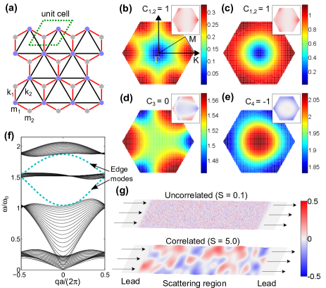
Figure 1: (a) Schematic of the hexagonal lattice. The blue (gray) circles represent the masses $m_{1}$ ($m_{2}$) while the red (black) lines represent the linear springs $k_{1}$ ($k_{2}$). (b)-(e) Plot of the first to fourth phonon band over the first Brillouin zone (BZ). The units of the color scale are in $\omega_{0}$. The accompanying insets show the Berry fluxes $F_{n}^{xy}$ with their corresponding Chern numbers ($C_{n}$, $n=$ 1 to 4). We combine the Chern number ($C_{1,2}$) for the first two bands because they are degenerate at the BZ center. (f) Phonon dispersion for $N_{W}=20$ lattice waveguide. (g) Schematic of uncorrelated and correlated mass disorder in a waveguide. The color scale for $\delta m(\mathbf{r})$ is shown.

II.2 Topological phononic lattice waveguide configuration

To simulate the transport of TPE and non-TPE modes, we set up the lattice waveguide with a finite mass-disordered scattering region of length $N_{L}a$ sandwiched between two pristine semi-infinite leads. $N_{L}$ is the number of unit cells spanning the scattering region and $a$ is the 1D lattice constant. Disorder in the scattering region is introduced by modifying the mass $m(\mathbf{r})$ at each site $\mathbf{r}$ by a random variable $\delta m(\mathbf{r})$, i.e., $m(\mathbf{r})=\langle m\rangle+\delta m(\mathbf{r})$ where $\langle m\rangle=1.0$. The spatial correlation in $\delta m(\mathbf{r})$ is characterized by the function

$$\langle\delta m(\mathbf{r}_{1})\delta m(\mathbf{r}_{2})\rangle=\langle\delta m^{2}\rangle\exp[-|\mathbf{r}_{1}-\mathbf{r}_{2}|^{2}/(2S^{2})]\ ,$$ (2)

where $S$ is the correlation length and $\langle\ldots\rangle$ is the ensemble average. The detailed procedure for generating the correlated disorder in Eq. (2) is described in Appendix A. We note that the mass disorder results in the changes in the diagonal and off-diagonal matrix elements of the “Hamiltonian” $\mathbf{M^{-1/2}KM^{-1/2}}$. Such mass disorder in the scattering region can be realized experimentally by using ‘atoms’ of different masses in the lattice Wang et al. (2015); Nash et al. (2015). The mass $m(\mathbf{r})$ is treated as a continuous random variable like in other studies of disordered harmonic lattices Li et al. (2001); Chaudhuri et al. (2010); Pinski et al. (2012). We set the nearest-neighbor distance between the masses $r_{\textrm{NN}}$ to $1.0$. We take $S=0.1$ to represent uncorrelated disorder, since $S\ll r_{\textrm{NN}}$, and $S=5.0$ to represent correlated disorder. The root-mean-square mass disorder is set as $\sqrt{\langle\delta m^{2}\rangle}=0.1$. Figure 1(g) shows the spatial profile of $\delta m(\mathbf{r})$ for $S=0.1$ and $S=5.0$, with the latter showing significant domains of positive ($\delta m>0$, in red) or negative ($\delta m<0$, in blue) mass disorder. In the waveguide, incoming left lead phonons are either reflected from or scattered across the disordered scattering region to the available right-lead channels. Due to transverse subband quantization, there are $N(\omega)$ transmitting and receiving channels at each frequency. The calculated transmission coefficient (TC) of each left-lead mode, $\Xi_{n}(\omega)$ for $n=1,\ldots,N(\omega)$, gives the fraction of energy that is transmitted after scattering. We define the transmittance $T(\omega)$ as the sum of the TCs at each frequency, i.e. $T(\omega)=\sum_{n=1}^{N(\omega)}\Xi_{n}(\omega)$.

III Results and discussion

III.1 Effect of disorder correlation on transmission coefficients

We first consider the case of uncorrelated disorder ($S=0.1$). Since translational symmetry is still preserved after disorder averaging, the Chern number remains well-defined in momentum space and the TPE states are robust. This is evident from Figs. 2 (a) and (c), which show the phonon dispersion with the computed average mode transmission coefficients superimposed on it. The TC is close to unity for the TPE modes in the two yellow-shaded frequency ranges, each of which delineates a “topological band gap” (TBG). The lower TBG ($1.15<\omega/\omega_{0}<1.45$) lies between the second and third bands [Figs. 1(c) and (d)] and the upper TBG ($1.575<\omega/\omega_{0}<1.825$) lies between the third and fourth bands [Figs. 1(d) and (e)]. The topological mode TCs show no appreciable decrease as the waveguide length is increased ten times from $N_{L}=200$ to $2000$, attesting to their immunity to backscattering.

The TCs for the bulk (non-TPE) modes with uncorrelated disorder exhibit the following universal behavior. Notably, the TC in each branch decreases at higher frequencies, a tendency also observed in disordered single-channel atomic chains Matsuda and Ishii (1970); Dhar (2001); Ong and Zhang (2014a, b). As expected, the TCs decrease as the size of the system increases from $N_{L}=200$ [Fig. 2(a)] to $2000$ [Fig. 2(c)], indicating that transmission is attenuated by the length of the intervening disordered medium. More interestingly, at the same frequency, the TC is generally lower for modes nearer to the BZ center ($q=0$) and with smaller group velocities, indicating that slower modes are more strongly attenuated by disorder.

When spatial correlation [Eq. (2)] is introduced in the disorder, the system effectively becomes a conglomerate of “islands” with different masses, and translational symmetry is broken even after disorder averaging. Consequently, the TCs for non-TPE modes are enhanced (reduced) at higher (lower) frequencies below the bottom edge of the lower TBG, i.e., for $\omega/\omega_{0}<1.15$. This is evident from comparing Figs. 2(b) and (d), where $S=5.0$, with Figs. 2(a) and (c) with $S=0.1$. Additional results showing the change in TC with correlation length are given in Appendix C. The most striking effect of disorder correlation is the transmission attenuation of states that are topologically protected when the disorder is uncorrelated. In Figs. 2(c) and (d), we observe considerable reduction of the TC in former TPE states within the upper TBG, with the reduction more pronounced near the band gap edges. This is related to the breakdown of a single bulk Chern number and the onset of bulk localization.

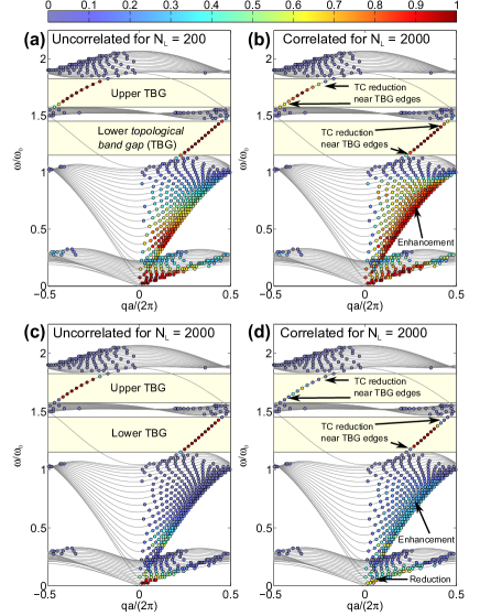
Phonon modes	Phonon mode transmission $\Xi_{n}$
	Higher $q$	Higher $\omega$	Higher $S$
Low-frequency	Enhanced	Reduced	Reduced
(bulk)
High-frequency			Enhanced
(bulk)
Topologically	Enhanced, if mode shifts		Reduced
protected edge	away from TBG edge

Figure 2: Average phonon mode transmission coefficients for $N_{L}=200$ with (a) uncorrelated and (b) correlated disorder. The transmission coefficients have a value between 0 and 1, and are indicated by color according to the top color bar scale. The effects of correlated disorder on the transmission attenuation can be seen more clearly for $N_{L}=2000$ with (c) uncorrelated and (d) correlated disorder. The yellow-shaded bands represent the topological band gaps. Since the propagation direction is rightward, only modes with a positive group velocity ($\partial\omega/\partial q>0$) can be transmitted. The table summarizes the effects of changing the wave vector ($q$), frequency ($\omega$) and disorder correlation length ($S$) on the transmission coefficients $\Xi_{n}$ for different phonon modes. More plots for $S=1.0$ and $2.0$ are available in Appendix C.

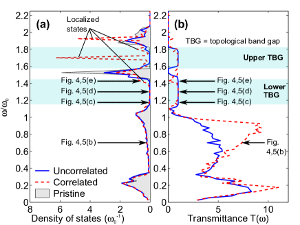
Figure 3: (a) Total density of states $\overline{\rho}(\omega)$ spectra for the scattering region in the $N_{L}=200$ waveguide with uncorrelated (solid line), correlated (dashed line) and no disorder (pristine). (b) The corresponding transmittance spectra for uncorrelated and correlated disorder. The corresponding local density of states for $\omega/\omega_{0}$ = 0.700, 1.175, 1.300 and 1.425 are shown in Figs. 4 and 5(b)-(e) and labeled accordingly.

III.2 Changes in transmission coefficients and density of states

The topological mode TC reduction from correlated disorder suggests coupling between the propagating states from the leads and the localized states within the scattering region. It is known that the amplitude of a mode localized within the the interior of a disordered region is exponentially small at the boundary and couples weakly to the surrounding degrees of freedom at the boundaries Shi et al. (2015), reducing the probability of an incoming propagating mode being transmitted across the disordered scattering region. To clarify the relationship between correlated disorder and the formation of the localized states, we compare the local density of states (LDOS) $\rho(\omega,\mathbf{r})$, defined in B.7, for both uncorrelated and correlated disorder (Figs. 4 and 5 respectively) at the specific frequencies indicated in Fig. 3, in which their total density of states (TDOS) $\overline{\rho}(\omega)$, defined as

$$\overline{\rho}(\omega)=\frac{\int d\mathbf{r^{\prime}}\rho(\omega,\mathbf{r^{\prime}})\sum_{\mathbf{r}}\delta(\mathbf{r^{\prime}}-\mathbf{r})}{d\omega\int d\mathbf{r^{\prime}}\rho(\omega,\mathbf{r^{\prime}})\sum_{\mathbf{r}}\delta(\mathbf{r^{\prime}}-\mathbf{r})}$$ (3)

where $\rho(\omega,\mathbf{r})$ is given in Eq. (29) and the summation $\sum_{\mathbf{r}}\ldots$ is over lattice degrees of freedom within the scattering region, and corresponding transmittance spectra $T(\omega)$ are shown for a single $N_{L}=200$ realization. The TDOS $\overline{\rho}(\omega)$ corresponds to the normalized average LDOS within the disordered region and satisfies the relation $\int d\omega\overline{\rho}(\omega)=1$.

As expected, uncorrelated disorder localizes bulk states, leading to reduced bulk transmission, but leaves the TPE states unattenuated. At $\omega/\omega_{0}=0.700$ in the bulk transmission window, the LDOS is well-localized with stripe-like patterns within the bulk of the waveguide because of the uncorrelated disorder [Fig. 4(b)]. However, near the bottom [Fig. 4(c)] and middle [Fig. 4(d)] of the lower TBG, only TPE modes exist and the LDOS is consistently edge-localized in spite of the disorder. There is some accumulation of bulk-localized states nearer to the top edge of the lower TBG [Fig. 4(e)], but that is not sufficient to destroy the near-perfect transmission. We associate the absence of significant bulk localization in the TBGs [Figs. 4(c)-(e)] with near-perfect transmittance ($T(\omega)\geq 0.99$).

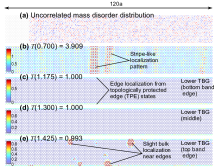
Figure 4: (a) Uncorrelated mass disorder distribution in a portion of an $N_{L}=200$ waveguide with positive (red) and negative (blue) $\delta m$. Part of the left lead is also shown. The shading intensity corresponds to the amplitude of the $\delta m(\mathbf{r})$. (b)-(e) The local density of states for $\omega/\omega_{0}=$ 0.700, 1.175, 1.300 and 1.425 are shown together with their transmittance $T(\omega)$ values. (c)-(e) correspond to modes in the lower TBG. Bulk localization only occurs in the bulk window [(b)], and to a small extent near the TBG [(e)].

When disorder is spatially correlated [Fig. 5(a)], there exists heterogeneous regions of mass domains that are large enough to be topologically distinct. This is most apparent in the LDOS spectra within the TBGs, where bulk states do not exist in the pristine case. But here, near the bottom of the lower TBG [Fig. 5(c)], parts of the LDOS are localized inside the bulk and confined within the $\delta m<0$ domains delineated by the unshaded portions of Fig. 5(c), implying that the bulk-localized states are formed within the $\delta m<0$ domains. At $\omega/\omega_{0}=1.300$ in the middle of the lower TBG [Fig. 5(d)], there is no bulk localization although it is again observed near the top of the lower TBG [Fig. 5(e)]. However, unlike Fig. 5(c), the contiguous bulk-localized portions are confined within the $\delta m>0$ domains. The difference between the LDOS spectra in Figs. 5(c)-(e) suggests that the correspondence in the spatial distribution of the bulk-localized states and the mass disorder domains is frequency-sensitive.

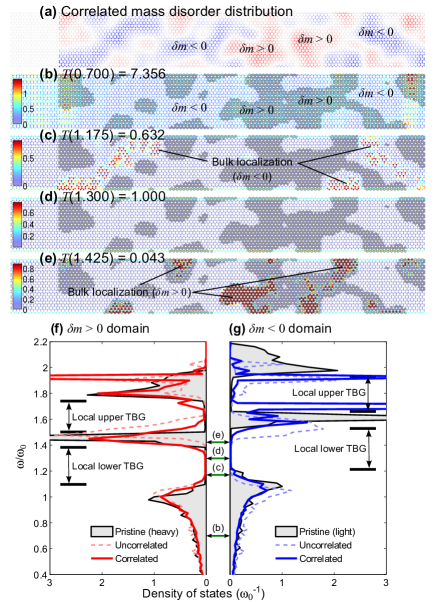
Figure 5: (a) Plot of $\delta m(\mathbf{r})$ like in Fig. 4 but for a realization of correlated disorder, with positive (red) and negative (blue) $\delta m$. (b)-(e) The local density of states (LDOS) at $\omega/\omega_{0}=$ 0.700, 1.175, 1.300 and 1.425 are shown together with their transmittance $T(\omega)$ values. The sites in (b)-(e) corresponding to $\delta m>0$ are outlined with a solid gray line in the background. In the bulk window, the LDOS is well-localized within the bulk like in Fig. 4(b), but there is no direct correspondence between the localized LDOS regions and the mass disorder domains. (f) The LDOS averaged over sites with $\delta m>0$ for uncorrelated (dashed line) and correlated (solid line) disorder, and the TDOS for the pristine (heavy) system with a mass shift of $\langle m\rangle\rightarrow\langle m\rangle+\sqrt{\langle\delta m^{2}\rangle}$. (g) The LDOS averaged over sites with $\delta m<0$ for uncorrelated and correlated disorder, and the TDOS for the pristine (light) system with a mass shift of $\langle m\rangle\rightarrow\langle m\rangle-\sqrt{\langle\delta m^{2}\rangle}$. The corresponding shifted local TBGs for (f) and (g) are also indicated.

III.3 Bulk localization and local topological band gap shifts

Having established the basic picture of how bulk localization [Figs. 5(b)-(e)] depends on domain distribution [Fig. 5(a)], we connect it to the change in density of states and transmittance in Figs. 3(a) and (b). It is heuristically useful to interpret the $\delta m>0$ ($\delta m<0$) domains as islands with positive (negative) mass ‘doping’ that downshifts (upshifts) the local TBGs. At the bottom edge of the lower TBG [Fig. 5(c)], the states in the $\delta m>0$ domains are in the downshifted local TBG and are thus ‘TPE-like’ while the states in the $\delta m<0$ domains are outside of the upshifted local TBG and can be described as ‘bulk-like’. Thus, the bulk-localized states in Fig. 5(c) only occur in the $\delta m<0$ domains. Similarly, at the top edge of the lower TBG [Fig. 5(e)], the states in the $\delta m>0$ domains are just above the top edge of the downshifted local TBG and ‘bulk-like’ while the states in the $\delta m<0$ domains are inside the upshifted local TBG and ‘TPE-like’. Hence, the bulk localization [Fig. 5(e)] occurs only in the $\delta m>0$ domains.

To illustrate this explanation, we plot in Fig. 5(f) the LDOS averaged over the heavier $\delta m>0$ sites for correlated [Figs. 4(a)] and uncorrelated [Fig. 5(a)] disorder. The spectra are similar at low frequencies but diverge as $\omega\rightarrow\infty$. In particular, the correlated-disorder LDOS gap is downshifted with respect to the TBGs in Fig. 3(a). We interpret the shift as the local TBG downshift caused by positive mass loading. To confirm this interpretation, we plot the TDOS for a heavy pristine system with a positive mass shift of $\langle m\rangle\rightarrow\langle m\rangle+\sqrt{\langle\delta m^{2}\rangle}$. The TDOS is much better aligned to the LDOS for correlated ($\delta m>0$) disorder than for uncorrelated disorder, reinforcing the idea that the gap downshift is due to the mass loading of the local modes within the $\delta m>0$ domains. Likewise, we also plot the LDOS averaged over the lighter $\delta m<0$ sites in Figs. 4(a) and 5(a) together with the TDOS for a light pristine system with a negative mass shift of $\langle m\rangle\rightarrow\langle m\rangle-\sqrt{\langle\delta m^{2}\rangle}$. Similarly, the light pristine TDOS is much better aligned to the average LDOS for correlated ($\delta m<0$) disorder than for uncorrelated disorder. Finally, in contrast, the gaps in the LDOS spectra for uncorrelated disorder $\delta m>0$ [Fig. 5(f)] and $\delta m<0$ [Fig. 5(g)] are well-aligned to each other and to the TBGs in Fig. 3(a), confirming that mass loading has less effect on their TBGs.

IV Summary and conclusions

We have studied the transmission of topological protected edge (TPE) and non-topological bulk modes through a finite mass-disordered lattice waveguide and found that correlated mass disorder enhances (reduces) the transmission of high (low) frequency non-topological modes. However, the transmission of TPE modes near the band edges of topological band gap (TBG) is degraded by correlated disorder because of the formation of bulk-localized states in topologically distinct mass ($\delta m>0$ and $\delta m<0$ ) domains in which one can effectively define a shifted local topological band gap. We find that bulk localization in the mass domain is only permitted if the mode frequency lies outside of the local TBG. This suggests that we can control the spatial localization of acoustic energy in a topological phononic crystal through correlated disorder.

Appendix A Generation of correlated mass disorder

We first generate a dense two-dimensional (2D) Cartesian grid in the $x$-$y$ plane for the Gaussian function

$$f(x,y)=\frac{1}{\pi S^{2}}\exp\left(-\frac{x^{2}+y^{2}}{S^{2}}\right)$$ (4)

over the domain where $-\frac{D}{2}<x\leq\frac{D}{2}$ and $-\frac{D}{2}<y\leq\frac{D}{2}$ for $D\gg S$. The Fourier components $\tilde{f}(k_{x},k_{y})=\mathcal{F}[f(x,y)]$ are computed by taking the discrete Fourier transform. We then multiply each Fourier component by a random phase factor $\theta(k_{x},k_{y})$ uniformly distributed between $0$ and $2\pi$:$\tilde{f}(k_{x},k_{y})\rightarrow\tilde{f}(k_{x},k_{y})e^{i\theta(k_{x},k_{y})}$. The 2D random function $h(x,y)$ is obtained by taking the real part of the inverse Fourier transform of $\tilde{f}(k_{x},k_{y})e^{i\theta(k_{x},k_{y})}$, i.e.,

$$h(x,y)=\sqrt{2}\text{Re}\mathcal{F}^{-1}[\tilde{f}(k_{x},k_{y})e^{i\theta(k_{x},k_{y})}]\ .$$ (5)

Figure 6 shows the spatial profile of $f(x,y)$ and $h(x,y)$, with the latter displaying distinct domains. It can be shown that the autocorrelation function of $h(x,y)$ has a Gaussian form, i.e.,

$$\frac{\langle h(x,y)h(0,0)\rangle}{\langle h(0,0)^{2}\rangle}=\exp\left(-\frac{x^{2}+y^{2}}{2S^{2}}\right)\ ,$$

where $\langle\ldots\rangle$ represents the average taken over all disorder realizations. Therefore, the mass disorder at site $\mathbf{r}=(x,y)$ is given by

$$\delta m(\mathbf{r})=\sqrt{\frac{\langle\delta m\rangle}{\langle h(0,0)^{2}\rangle}}h(x,y)\ .$$ (6)

Roughly speaking, the length scale of the domains in $h(x,y)$ is $\sim 2S$.

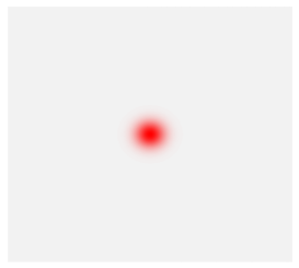
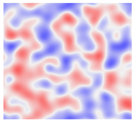
Figure 6: The left shows the function $f(x,y)=\frac{1}{\pi S^{2}}\exp\left(-\frac{x^{2}+y^{2}}{S^{2}}\right)$ from Eq. (4) while the right shows the function $h(x,y)$ from Eq. (5) for $S=5.0$.

We note that the above approach can be generalized to arbitrarily correlated textures. Suppose we start from a generic distribution $f(\mathbf{r})$. We want to derive the spatial correlation of $h(\mathbf{r})=\sqrt{2}\text{Re}\mathcal{F}^{-1}[\tilde{f}(\mathbf{k})e^{i\theta(\mathbf{k})}]$, i.e. the inverse Fourier transform of the product of the Fourier transform of $f$ with a random phase. We have

$$\langle h(\mathbf{r}+\Delta\mathbf{r})h(\mathbf{r})\rangle = \frac{1}{2}\left\langle\left(\int e^{i\mathbf{k}\cdot(\mathbf{r}+\Delta\mathbf{r})}e^{i\theta(\mathbf{k})}f(\mathbf{k})d\mathbf{k}+\text{c.c}\right)\left(\int e^{i\mathbf{k}^{\prime}\cdot\mathbf{r}}e^{i\theta(\mathbf{k}^{\prime})}f(\mathbf{k}^{\prime})d\mathbf{k}^{\prime}+\text{c.c}\right)\right\rangle$$

$$= \frac{1}{2}\left(\int\int\langle e^{i(\theta(\mathbf{k})+\theta(\mathbf{k}^{\prime}))}\rangle e^{i(\mathbf{k}\cdot(\mathbf{r}+\Delta\mathbf{r})+\mathbf{k}^{\prime}\cdot\mathbf{r})}f(\mathbf{k})f(\mathbf{k}^{\prime})d\mathbf{k}d\mathbf{k}^{\prime}+\text{c.c}\right)$$

$$+\frac{1}{2}\left(\int\int\langle e^{i(\theta(\mathbf{k})-\theta(\mathbf{k}^{\prime}))}\rangle e^{i(\mathbf{k}\cdot(\mathbf{r}+\Delta\mathbf{r})-\mathbf{k}^{\prime}\cdot\mathbf{r})}f(\mathbf{k})\bar{f}(\mathbf{k}^{\prime})d\mathbf{k}d\mathbf{k}^{\prime}+\text{c.c}\right)$$

$$= \int\cos(\mathbf{k}\cdot\Delta\mathbf{r})|f(\mathbf{k})|^{2}d\mathbf{k}$$

$$= \text{Re}\left[\int f(\mathbf{r}+\Delta\mathbf{r})\bar{f}(\mathbf{r})d\mathbf{r}\right]$$

which is just the real part of the convolution of $f$. In going to line 4, we have made use of the fact that $\langle e^{i(\theta(\mathbf{k})+\theta(\mathbf{k}^{\prime}))}\rangle=0$ and $\langle e^{i(\theta(\mathbf{k})-\theta(\mathbf{k}^{\prime}))}\rangle=\delta_{\mathbf{k},\mathbf{k}^{\prime}}$, since $\theta$ is uncorrelated with $\mathbf{k}$. Indeed, the random phase ’randomizes’ $f(\mathbf{r})$, replacing the convolution with the autocorrelation function. This result can also be extended to higher correlations of even orders.

If given a desired correlation function $\langle h(\mathbf{r})h(\mathbf{0})\rangle$, one can find the requisite initial distribution via

$$f(\mathbf{r})=\int e^{i\mathbf{k}\cdot\mathbf{r}}\sqrt{\int e^{-i\mathbf{k}\cdot\mathbf{r}^{\prime}}\langle h(\mathbf{r})h(\mathbf{0})\rangle d\mathbf{r}^{\prime}}d\mathbf{k}$$ (7)

In this paper, the Gaussian distribution has the special property that its autocorrelation is still a Gaussian, albeit with twice the variance:

$$\int e^{-(x+\Delta x)^{2}}e^{-x^{2}}dx=e^{-\frac{(\Delta x)^{2}}{2}}$$

Appendix B Calculation of mode transmission coefficient and local density of states

Our computation of the transmission coefficient is adapted from the extension of the commonly used nonequilibrium Green’s function method described in Ong and Zhang Ong and Zhang (2015). Although the approach was originally proposed for the study of nanoscale interfacial phonon transmission, the structure of the equations describing the topological lattice waveguide is in fact identical to that of the equations typically used to model nanoscale phonons and is thus compatible with the method, allowing us to apply the method to the macroscopic topological phononic lattice system.

In the method, the one-dimensional (1D) system is divided into three parts: the left lead, the central scattering region and the right lead. The finite width of the leads means that the waveguide can be treated as a multichannel system. At each frequency, a propagating mode in the left lead is treated as a transmitting channel while a propagating mode in the right lead is a receiving channel. Numerically, the system identifies and extracts the eigenmodes of the left and right lead from the uncoupled surface Green’s function of the respective leads. The retarded Green’s function relating the left and right edges of the scattering region is also computed and then used to calculate the transition amplitude between each transmitting channel and each receiving channel. Formally, this is equivalent to calculating the scattering amplitude between the left lead modes and the right lead modes.

B.1 Structure and geometry of lattice waveguide

The width of the waveguide is $N_{W}=20$ unit cells across and its length is $2N+N_{L}$ unit cells. Hence, each cell (or principal layer) of the waveguide consists of $20$ unit cells. As shown in Fig. 7, the waveguide can be divided into three components: the pristine left lead, the scattering region with disorder and the pristine right lead. There are $N$ cells in each lead and $N_{L}$ cells in the scattering region. We enumerate the cells from $n=N^{-}$ to $n=N^{+}$ where $N^{-}=-N+1$ and $N^{+}=N_{L}+N$ . Although we will take the limit $N\rightarrow\infty$ eventually, we treat $N$ as a finite number in the following description of the setup of the matrices and equations.

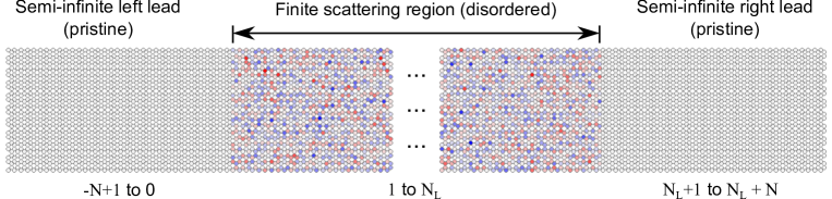
Figure 7: Schematic of the different components of the lattice waveguide: the left lead, the scattering region and the right lead. The enumeration of the cells in each component is also given.

B.2 Equation of motion

The equation of motion for the entire lattice waveguide can be compactly written as

$$\left(\mathbf{M}\frac{d^{2}}{dt^{2}}-\mathbf{K}\right)\mathbf{U}=\mathbf{0}$$ (8)

where $\mathbf{K}$ and $\mathbf{M}$ are the stiffness and mass matrices, respectively, and $\mathbf{U}$ is the column vector of displacement coordinates. The stiffness matrix in Eq. (8) can be written in the block-tridiagonal form with diagonal and off-diagonal bands of submatrices,

$$\mathbf{K}=\left(\begin{array}[]{cccccc}\boldsymbol{K}_{N^{-},N^{-}}&\boldsymbol{K}_{N^{-},N^{-}+1}\\ \boldsymbol{K}_{N^{-}+1,N^{-}}&\ddots&\ddots\\ &\ddots&\boldsymbol{K}_{n,n}&\boldsymbol{K}_{n,n+1}\\ &&\boldsymbol{K}_{n+1,n}&\ddots&\ddots\\ &&&\ddots&\boldsymbol{K}_{N^{+}-1,N^{+}-1}&\boldsymbol{K}_{N^{+}-1,N^{+}}\\ &&&&\boldsymbol{K}_{N^{+},N^{+}-1}&\boldsymbol{K}_{N^{+},N^{+}}\end{array}\right)$$ (9)

where each $\boldsymbol{K}_{n,m}$ is an $80\times 80$ submatrix and $n$ ($m=n\pm 1$) is the column (row) group index representing the position of the cell. Since the spring coupling between adjacent cells is identical, we set $\boldsymbol{K}_{n,n}=\boldsymbol{K}_{0,0}$, $\boldsymbol{K}_{n,n+1}=\boldsymbol{K}_{0,1}$ and $\boldsymbol{K}_{n,n-1}=\boldsymbol{K}_{1,0}$ for $n=N^{-},\ldots,N^{+}$. In addition, it follows from the Hermiticity of $\mathbf{K}$ that $\boldsymbol{K}_{n+1,n}=(\boldsymbol{K}_{n,n+1})^{\dagger}$.

The mass matrix in Eq. (8) can be expressed as

$$\mathbf{M}=\left(\begin{array}[]{ccccc}\boldsymbol{M}_{N^{-}}\\ &\ddots\\ &&\boldsymbol{M}_{1}\\ &&&\ddots\\ &&&&\boldsymbol{M}_{N^{+}}\end{array}\right)$$ (10)

where $\boldsymbol{M}_{n}$ is an $80\times 80$ submatrix representing the effective mass of the $n$-th cell for $n=N^{-},\ldots,N^{+}$. However, unlike Eq. (9), the masses associated with each cell are not necessarily periodic although the submatrices for the pristine left lead ($N^{-}\leq n\leq 0$) and right lead ($N_{L}+1\leq n\leq N^{+}$) are identical,i.e., $\boldsymbol{M}_{n}=\boldsymbol{M}_{0}$ for $N^{-}\leq n<1$ and $N_{L}<n\leq N^{+}$. The submatrices in the central scattering region ($1\leq n\leq N_{L}$) are however not identical because of mass disorder. Each of the submatrices $\boldsymbol{M}_{n}$ in the central scattering region ($1\leq n\leq N_{L}$) can be written in the block-diagonal form

$$\boldsymbol{M}_{n}=\left(\begin{array}[]{ccc}\boldsymbol{m}(\mathbf{r}_{1})\\ &\ddots\\ &&\boldsymbol{m}(\mathbf{r}_{40})\end{array}\right)$$ (11)

where $\mathbf{r}_{l}$ is the position of $l$-th mass within the cell, and

$$\boldsymbol{m}(\mathbf{r})=[\langle m\rangle+\delta m(\mathbf{r})]\left(\begin{array}[]{cc}1&-i\alpha\\ i\alpha&1\end{array}\right)$$ (12)

is the $2\times 2$ matrix representing the effective mass at $\mathbf{r}$ with $\alpha=0.3$ like in Ref. Wang et al. (2015). Equation (8) can be simplified to the matrix equation that is second order in time, i.e.

$$\left(\frac{d^{2}}{dt^{2}}+\mathbf{H}\right)\mathbf{V}=\mathbf{0}$$ (13)

where $\mathbf{V=\mathbf{M}}^{1/2}\mathbf{U}$, and $\mathbf{H}=\mathbf{M}^{-1/2}\mathbf{K}\mathbf{M}^{-1/2}$ is the mass-normalized force constant matrix that can be written in the block-tridiagonal form

$$\mathbf{H}=\left(\begin{array}[]{cccccc}\boldsymbol{H}_{N^{-},N^{-}}&\boldsymbol{H}_{N^{-},N^{-}+1}\\ \boldsymbol{H}_{N^{-}+1,N^{-}}&\ddots&\ddots\\ &\ddots&\boldsymbol{H}_{1,1}&\boldsymbol{H}_{1,2}\\ &&\boldsymbol{H}_{2,1}&\ddots&\ddots\\ &&&\ddots&\boldsymbol{H}_{N^{+}-1,N^{+}-1}&\boldsymbol{H}_{N^{+}-1,N^{+}}\\ &&&&\boldsymbol{H}_{N^{+},N^{+}-1}&\boldsymbol{H}_{N^{+},N^{+}}\end{array}\right)\ .$$ (14)

Each submatrix $\boldsymbol{H}_{n,m}$ is given by $\boldsymbol{H}_{n,m}=\boldsymbol{M}_{n}^{-1/2}\boldsymbol{K}_{n,m}\boldsymbol{M}_{m}^{-1/2}$ where $m=n$ or $n\pm 1$. The Hermiticity of $\mathbf{H}$ implies that $\boldsymbol{H}_{n,m}=(\boldsymbol{H}_{m,n})^{\dagger}$.

B.3 Division of waveguide into scattering region and leads

We recall in Fig. 7 that the scattering region corresponds to the cells for $1\leq n\leq N_{L}$ while the left (right) lead corresponds to the cells for $N^{-}\leq n\leq 0$ ($N_{L}+1\leq n\leq N^{+}$). In the left and right lead, there is no mass disorder or $\delta m(\mathbf{r})=0$ while in the scattering region, it is determined by Eq. (6). We can write Eq. (14) as

$$\mathbf{H}=\left(\begin{array}[]{ccc}\mathbf{H}_{L}&\mathbf{H}_{LC}\\ \mathbf{H}_{CL}&\mathbf{H}_{C}&\mathbf{H}_{CR}\\ &\mathbf{H}_{RC}&\mathbf{H}_{R}\end{array}\right)$$ (15)

where

$$\mathbf{H}_{L}=\left(\begin{array}[]{cccc}\boldsymbol{H}_{N_{-},N_{-}}&\boldsymbol{H}_{N_{-},N_{-}+1}\\ \boldsymbol{H}_{N_{-}+1,N_{-}}&\ddots&\ddots\\ &\ddots&\boldsymbol{H}_{-1,-1}&\boldsymbol{H}_{-1,0}\\ &&\boldsymbol{H}_{0,-1}&\boldsymbol{H}_{0,0}\end{array}\right)$$ (16a)

$$\mathbf{H}_{C}=\left(\begin{array}[]{cccc}\boldsymbol{H}_{1,1}&\boldsymbol{H}_{1,2}\\ \boldsymbol{H}_{2,1}&\boldsymbol{H}_{2,2}&\ddots\\ &\ddots&\ddots&\boldsymbol{H}_{N_{L}-1,N_{L}-1}\\ &&\boldsymbol{H}_{N_{L},N_{L}-1}&\boldsymbol{H}_{N_{L},N_{L}}\end{array}\right)$$ (16b)

$$\mathbf{H}_{R}=\left(\begin{array}[]{cccc}\boldsymbol{H}_{N_{L}+1,N_{L}+1}&\boldsymbol{H}_{N_{L}+1,N_{L}+2}\\ \boldsymbol{H}_{N_{L}+2,N_{L}+1}&\boldsymbol{H}_{N_{L}+2,N_{L}+2}&\ddots\\ &\ddots&\ddots&\boldsymbol{H}_{N_{+}-1,N_{+}}\\ &&\boldsymbol{H}_{N_{+},N_{+}-1}&\boldsymbol{H}_{N_{+},N_{+}}\end{array}\right)$$ (16c)

The matrices in Eqs. (16a), (16b) and (16c) correspond to the left lead, the scattering region and the right lead, respectively. The periodicity in the arrangement of the stiffness and mass matrices of the left lead implies that the diagonal and off-diagonal submatrices of Eq. (16a) satisfy the following conditions

$$\boldsymbol{H}_{N_{-},N_{-}}=\boldsymbol{H}_{N_{-}+1,N_{-}+1}=\ldots=\boldsymbol{H}_{0,0}$$

$$\boldsymbol{H}_{N_{-},N_{-}+1}=\boldsymbol{H}_{N_{-}+1,N_{-}+2}=\ldots=\boldsymbol{H}_{-1,0}$$

$$\boldsymbol{H}_{N_{-}+1,N_{-}}=\boldsymbol{H}_{N_{-}+2,N_{-}+1}=\ldots=\boldsymbol{H}_{0,-1}$$

Likewise, the diagonal and off-diagonal submatrices of Eq. (16c) also satisfy

$$\boldsymbol{H}_{N_{L}+1,N_{L}+1}=\ldots=\boldsymbol{H}_{N_{+},N_{+}}=\boldsymbol{H}_{0,0}$$

$$\boldsymbol{H}_{N_{L}+1,N_{L}+2}=\ldots=\boldsymbol{H}_{N_{+}-1,N_{+}}=\boldsymbol{H}_{-1,0}$$

$$\boldsymbol{H}_{N_{L}+2,N_{L}+1}=\ldots=\boldsymbol{H}_{N_{+},N_{+}-1}=\boldsymbol{H}_{0,-1}$$

Given the uniformity in the stiffness and mass submatrices, the dispersion ($\omega-\mu$) relationship for the propagating modes of the semi-infinite leads is determined by solving the equation

$$\det(\boldsymbol{H}_{0,-1}\lambda^{-1}+\boldsymbol{H}_{0,0}+\boldsymbol{H}_{0-1,0}\lambda-\omega^{2}\boldsymbol{I})=0$$ (17)

where $\boldsymbol{I}$ is the identity matrix and $\lambda=e^{i\mu a}$ is the Bloch factor. $\omega$ and $\mu$ are respectively the frequency and the wave vector. In the scattering region ($1\leq n\leq N_{L}$), the mass at each lattice site $m(\mathbf{r})=\langle m\rangle+\delta m(\mathbf{r})$ varies with the position $\mathbf{r}$ according to Eq. (6). The mass disorder of the scattering region causes the left lead propagating modes to be partially transmitted to the right lead.

B.4 Green’s functions for leads and scattering region

In the frequency domain, Eq. (15) becomes

$$(\omega^{2}\mathbf{I}-\mathbf{H})\tilde{\mathbf{V}}=\mathbf{0}$$ (18)

where $\tilde{\mathbf{V}}$ is the Fourier transform of $\mathbf{V}$ and $\mathbf{I}$ is the identity matrix. The retarded Green’s function corresponding to the linear operator in Eq. (18) is

$$\mathbf{G}^{\text{ret}}(\omega)=[(\omega^{2}+i0^{+})\mathbf{I}-\mathbf{H}]^{-1}$$ (19)

and Eq. (19) can be expressed as

$$\mathbf{G}^{\text{ret}}(\omega)=\left(\begin{array}[]{ccc}\mathbf{G}_{L}^{\text{ret}}(\omega)&\mathbf{G}_{LC}^{\text{ret}}(\omega)&\mathbf{G}_{LR}^{\text{ret}}(\omega)\\ \mathbf{G}_{CL}^{\text{ret}}(\omega)&\mathbf{G}_{C}^{\text{ret}}(\omega)&\mathbf{G}_{CR}^{\text{ret}}(\omega)\\ \mathbf{G}_{RL}^{\text{ret}}(\omega)&\mathbf{G}_{RC}^{\text{ret}}(\omega)&\mathbf{G}_{R}^{\text{ret}}(\omega)\end{array}\right)\ .$$

In order to compute the left lead mode transmission coefficients, we first need to find the retarded Green’s function $\mathbf{G}_{C}^{\text{ret}}(\omega)$ for the finite scattering region. It is given by the expression

$$\mathbf{G}_{C}^{\text{ret}}(\omega)=[(\omega^{2}+i0^{+})\mathbf{I}_{C}-\mathbf{H}_{C}^{\textrm{eff}}(\omega)]^{-1}\ ,$$ (20)

where the term $\mathbf{H}^{\textrm{eff}}(\omega)$ is the $\omega$-dependent effective Hamiltonian

$$\mathbf{H}_{C}^{\textrm{eff}}(\omega)=\mathbf{H}_{C}+\mathbf{H}_{CL}\mathbf{g}_{L}^{\text{ret}}(\omega)\mathbf{H}_{LC}+\mathbf{H}_{CR}\mathbf{g}_{R}^{\text{ret}}(\omega)\mathbf{H}_{RC}$$ (21)

with

$$\mathbf{g}_{L}^{\text{ret}}(\omega)=[(\omega^{2}+i0^{+})\mathbf{I}_{L}-\mathbf{H}_{L}]^{-1}$$

$$\mathbf{g}_{R}^{\text{ret}}(\omega)=[(\omega^{2}+i0^{+})\mathbf{I}_{R}-\mathbf{H}_{R}]^{-1}$$

The LHS of Eq. (21) can be written more explicitly as

$$\mathbf{H}_{C}^{\textrm{eff}}(\omega)=\left(\begin{array}[]{cccc}\boldsymbol{H}_{1,1}^{\textrm{eff}}&\boldsymbol{H}_{1,2}\\ \boldsymbol{H}_{2,1}&\boldsymbol{H}_{2,2}&\ddots\\ &\ddots&\ddots&\boldsymbol{H}_{N_{L}-1,N_{L}}\\ &&\boldsymbol{H}_{N_{L},N_{L}-1}&\boldsymbol{H}_{N_{L},N_{L}}^{\textrm{eff}}\end{array}\right)\ ,$$ (22)

with

$$\boldsymbol{H}_{1,1}^{\textrm{eff}}=\boldsymbol{H}_{1,1}+\boldsymbol{H}_{1,0}\boldsymbol{g}_{0,0}^{\text{ret}}(\omega)\boldsymbol{H}_{0,1}$$

and

$$\boldsymbol{H}_{N_{L},N_{L}}^{\textrm{eff}}=\boldsymbol{H}_{N_{L},N_{L}}+\boldsymbol{H}_{N_{L},N_{L}+1}\boldsymbol{g}_{N_{L}+1,N_{L}+1}^{\text{ret}}(\omega)\boldsymbol{H}_{N_{L}+1,N_{L}}\ .$$

The matrices $\boldsymbol{g}_{0,0}^{\text{ret}}(\omega)$ and $\boldsymbol{g}_{N_{L}+1,N_{L}+1}^{\text{ret}}(\omega)$ represent the surface Green’s function of the uncoupled left and right lead, respectively, and in the limit $N\rightarrow\infty$ where the leads become infinitely large, they satisfy the equations

$$\boldsymbol{g}_{0,0}^{\text{ret}}(\omega)= [(\omega^{2}+i0^{+})\boldsymbol{I}-\boldsymbol{H}_{0,0}$$

$$-\boldsymbol{H}_{0,-1}\boldsymbol{g}_{0,0}^{\text{ret}}(\omega)\boldsymbol{H}_{-1,0}]^{-1}$$ (23a)

$$\boldsymbol{g}_{N_{L}+1,N_{L}+1}^{\text{ret}}(\omega)= [(\omega^{2}+i0^{+})\boldsymbol{I}-\boldsymbol{H}_{0,0}$$

$$-\boldsymbol{H}_{-1,0}\boldsymbol{g}_{N_{L}+1,N_{L}+1}^{\text{ret}}(\omega)\boldsymbol{H}_{0,-1}]^{-1}\ .$$ (23b)

The nonlinear equations in Eq. (23) can be solved numerically with the decimation technique Ong and Zhang (2015) to yield the surface Green’s functions $\boldsymbol{g}_{0,0}^{\text{ret}}(\omega)$ and $\boldsymbol{g}_{N_{L}+1,N_{L}+1}^{\text{ret}}(\omega)$.

B.5 Surface Green’s functions, Bloch matrices and eigenmodes

It is shown by Ong and Zhang Ong and Zhang (2015) that the constant-$\omega$ propagating and evanescent eigenmodes can be extracted from the surface Green’s functions. We first compute the corresponding Bloch matrices

$$\boldsymbol{F}_{L}^{\text{adv}}(-)^{-1}=[\boldsymbol{H}_{0,-1}\boldsymbol{g}_{0,0}^{\text{ret}}]^{\dagger}$$ (24a)

and

$$\boldsymbol{F}_{R}^{\text{ret}}(+)=\boldsymbol{g}_{N_{L}+1,N_{L}+1}^{\text{ret}}\boldsymbol{H}_{0,-1}\ .$$ (24b)

The matrices $\boldsymbol{U}_{L}^{\text{adv}}(-)$ and $\boldsymbol{U}_{R}^{\text{ret}}(+)$, in which the column vectors represent the extended and evanescent eigenmodes, are obtained by solving numerically the equations

$$\boldsymbol{F}_{L}^{\text{adv}}(-)\boldsymbol{U}_{L}^{\text{adv}}(-)=\boldsymbol{U}_{L}^{\text{adv}}(-)\boldsymbol{\Lambda}_{L}^{\text{adv}}(-)$$ (25a)

and

$$\boldsymbol{F}_{R}^{\text{ret}}(+)\boldsymbol{U}_{R}^{\text{ret}}(+)=\boldsymbol{U}_{R}^{\text{ret}}(+)\boldsymbol{\Lambda}_{R}^{\text{ret}}(+)\ .$$ (25b)

The matrices $\boldsymbol{\Lambda}_{L}^{\text{adv}}(-)$ and $\boldsymbol{\Lambda}_{R}^{\text{ret}}(+)$ are diagonal matrices with the diagonal elements equal to the Bloch factor $\lambda=\exp(\mp i\mu a)$ of the corresponding propagating eigenmodes, where $a$ is the one-dimensional lattice constant.

$$\boldsymbol{\Lambda}_{L}^{\text{adv}}(-)=\left(\begin{array}[]{cccc}\lambda_{1}&0\\ 0&\lambda_{2}&\ddots\\ &\ddots&\ddots&0\\ &&0&\lambda_{80}\end{array}\right)$$

Thus, the wave vector $\mu$ of the eigenmode can be easily determined from $\lambda$.

The group velocity matrices for the eigenmodes are

$$\boldsymbol{V}_{L}(+)= \frac{ia}{2\omega}\boldsymbol{U}_{L}^{\text{adv}}(-)^{\dagger}\boldsymbol{H}_{0,-1}$$

$$\times[\boldsymbol{g}_{0,0}^{\text{ret}}(\omega)-\boldsymbol{g}_{0,0}^{\text{ret}}(\omega)^{\dagger}]\boldsymbol{H}_{-1,0}\boldsymbol{U}_{L}^{\text{adv}}(-)$$ (26a)

and

$$\boldsymbol{V}_{R}(+)= \frac{ia}{2\omega}\mathbf{U}_{R}^{\text{ret}}(+)^{\dagger}\boldsymbol{H}_{-1,0}[\boldsymbol{g}_{N+1,N+1}^{\text{ret}}(\omega)$$

$$-\boldsymbol{g}_{N+1,N+1}^{\text{ret}}(\omega)^{\dagger}]\boldsymbol{H}_{0,-1}\boldsymbol{U}_{R}^{\text{ret}}(+)\ ,$$ (26b)

which are needed for calculating the transmission coefficient later. The off-diagonal elements of the velocity matrices in Eq. 26 are zero while the diagonal elements are positive only if the corresponding eigenmode is propagating (extended).

Like $\mathbf{H}_{C}^{\textrm{eff}}(\omega)$ in Eq. (22), the matrix $\mathbf{G}_{C}^{\text{ret}}(\omega)$ in Eq. (20) can be written in the block form

$$\mathbf{G}_{C}^{\text{ret}}(\omega)=\left(\begin{array}[]{cccc}\boldsymbol{G}_{1,1}^{\textrm{ret}}&\boldsymbol{G}_{1,2}^{\textrm{ret}}&\cdots&\boldsymbol{G}_{1,N_{L}}^{\textrm{ret}}\\ \boldsymbol{G}_{2,1}^{\textrm{ret}}&\boldsymbol{G}_{2,2}^{\textrm{ret}}&\ddots&\vdots\\ \vdots&\ddots&\ddots&\boldsymbol{G}_{N_{L}-1,N_{L}}^{\textrm{ret}}\\ \boldsymbol{G}_{N_{L},1}^{\textrm{ret}}&\cdots&\boldsymbol{G}_{N_{L},N_{L}-1}^{\textrm{ret}}&\boldsymbol{G}_{N_{L},N_{L}}^{\textrm{ret}}\end{array}\right)\ .$$

The submatrix $\boldsymbol{G}_{n,m}^{\textrm{ret}}(\omega)$ can be interpreted as the frequency-domain transfer function for the vibrational response at unit cell $n$ to an oscillatory harmonic driving force at unit cell $m$ with frequency $\omega$. Intuitively, information on energy transfer from the leftmost cell to the rightmost cell of the scattering region should be contained in the submatrix $\boldsymbol{G}_{N_{L},1}^{\textrm{ret}}(\omega)$.

B.6 Transmission amplitude matrix

The transmission amplitude matrix is

$$\boldsymbol{t}(\omega)= \frac{2i\omega}{a}\boldsymbol{V}_{R}(+)^{\nicefrac{{1}}{{2}}}[\boldsymbol{U}_{R}^{\text{ret}}(+)]^{-1}$$

$$\times\boldsymbol{\mathcal{G}}_{C}^{\text{ret}}(\omega)[\boldsymbol{U}_{L}^{\text{adv}}(-)^{\dagger}]^{-1}\boldsymbol{V}_{L}(+)^{\nicefrac{{1}}{{2}}}$$ (27)

where

$$\boldsymbol{\mathcal{G}}_{C}^{\text{ret}}(\omega)=\boldsymbol{g}_{N_{L}+1,N_{L}+1}^{\text{ret}}(\omega)\boldsymbol{H}_{0,-1}\boldsymbol{G}_{N_{L},1}^{\textrm{ret}}(\omega)\boldsymbol{H}_{0,-1}\boldsymbol{g}_{0,0}^{\text{ret}}(\omega)\ .$$

The individual matrix elements of the transmission matrix in Eq. (27) gives the transition probability amplitude between an in-coming left lead channel and an out-going right lead channel at frequency $\omega$. For instance, $t_{mn}$ gives the transition probability amplitude between the in-coming left lead eigenmode corresponding to the $n$-th column vector of $\boldsymbol{U}_{L}^{\text{adv}}(-)$, with its Bloch factor given by the $n$-th diagonal element of $\boldsymbol{\Lambda}_{L}^{\text{adv}}(-)$, and the out-going right lead eigenmode corresponding to the $m$-th column vector of $\boldsymbol{U}_{R}^{\text{ret}}(+)$ with its Bloch factor given by the $m$-th diagonal element of $\boldsymbol{\Lambda}_{R}^{\text{ret}}(+)$. If either one of the eigenmodes is an evanescent mode, then its group velocity is 0, i.e. $[\boldsymbol{V}_{L}(+)]_{n,n}=0$ or $[\boldsymbol{V}_{R}(+)]_{m,m}=0$, and the transition probability amplitude is $t_{mn}=0$.

The transmission coefficient of the $n$-th left lead eigenmode $\Xi_{n}(\omega)$ is given by $\Xi_{n}(\omega)=\sum_{m}|t_{mn}(\omega)|^{2}$, or the $n$-th diagonal element of $\boldsymbol{t}(\omega)^{\dagger}\boldsymbol{t}(\omega)$, and has a numerical value between 0 and 1. The associated wavevector $\mu$ can be determined by from the $n$-th diagonal element of $\boldsymbol{\Lambda}_{L}^{\text{adv}}(-)$ which yields the Bloch factor $\lambda=e^{i\mu a}$. The transmittance at frequency $\omega$ can be computed from the sum of the transmission coefficients, i.e.,

$$T(\omega)=\sum_{n}\Xi_{n}(\omega)=\text{Tr}[\boldsymbol{t}(\omega)^{\dagger}\boldsymbol{t}(\omega)]\ .$$ (28)

In the absence of any mass disorder in the scattering region, the transmittance in Eq. (28) is an integer equal to the number of channels in each lead at frequency $\omega$ since $\Xi_{n}(\omega)=1$ for each propagating eigenmode and $0$ otherwise.

B.7 Local density of states

The local density of states (LDOS) at site $\mathbf{r}$ in the scattering region is

$$\rho(\omega,\mathbf{r})=\frac{i\omega}{\pi a}\sum_{n(\mathbf{r})}[\mathbf{G}_{C}^{\text{ret}}(\omega)-\mathbf{G}_{C}^{\text{ret}}(\omega)^{\dagger}]_{n(\mathbf{r}),n(\mathbf{r})}$$ (29)

where $n(\mathbf{r})$ is the index of the degrees of freedom associated with site $\mathbf{r}$. In effect, Eq. (29) is the trace of a $2\times 2$ matrix, and the LDOS has the units of inverse length times inverse frequency. The scattering region has $N_{L}$ cells and each cell has $40$ lattice sites and $80$ degrees of freedom since each lattice site has two degrees of freedom, one in $x$ and the other in $y$. Hence, the entire scattering region has $80N_{L}$ degrees of freedom and $\mathbf{G}_{C}^{\text{ret}}$ is an $80N_{L}\times 80N_{L}$ matrix. To find the LDOS at a site of a particular site $\mathbf{r}$, we only need to sum over the two diagonal elements of $\mathbf{G}_{C}^{\text{ret}}$ corresponding to the $x$ and $y$ degrees of freedom at site $\mathbf{r}$. In total, there are $40N_{L}$ lattice sites $\mathbf{r}$ and associated LDOS values $\rho(\mathbf{r})$.

Appendix C Mode transmission coefficients for different correlation lengths

We plot the mode transmission coefficients in Fig. 8 for different values of the correlation length $S$ at $N_{L}=200$, $1000$ and $5000$. Figures 8(g) to (i) show that the mode transmission coefficients for the very low-frequency modes and the TPE modes in the lower and upper topological band gap (TBG) decrease as $S$ increases. On the other hand, the transmission of the higher-frequency modes is enhanced as we increase $S$.

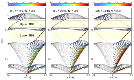
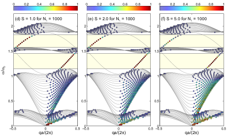
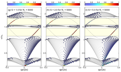
Figure 8: Mode transmission coefficients (color in the small circles) for correlation lengths $S=1.0$, $2.0$ and $5.0$ at (a-c) $N_{L}=200$, (d-f) $N_{L}=1000$ and (g-i) $N_{L}=5000$. The yellow-shaded regions correspond to the topological band gaps.

References

- Wang et al. (2015) P. Wang, L. Lu, and K. Bertoldi, Phys. Rev. Lett. 115, 104302 (2015).
- Khanikaev et al. (2015) A. B. Khanikaev, R. Fleury, S. H. Mousavi, and A. Alù, Nature Communications 6, 8260 (2015).
- Yang et al. (2015) Z. Yang, F. Gao, X. Shi, X. Lin, Z. Gao, Y. Chong, and B. Zhang, Phys. Rev. Lett. 114, 114301 (2015).
- Mousavi et al. (2015) S. H. Mousavi, A. B. Khanikaev, and Z. Wang, Nature Communications 6, 8682 (2015).
- Nash et al. (2015) L. M. Nash, D. Kleckner, A. Read, V. Vitelli, A. M. Turner, and W. T. Irvine, Proceedings of the National Academy of Sciences 112, 14495 (2015).
- Süsstrunk and Huber (2015) R. Süsstrunk and S. D. Huber, Science 349, 47 (2015).
- Fu and Kane (2007) L. Fu and C. L. Kane, Phys. Rev. B 76, 045302 (2007).
- Fu et al. (2007) L. Fu, C. L. Kane, and E. J. Mele, Phys. Rev. Lett. 98, 106803 (2007).
- Qi et al. (2008) X.-L. Qi, T. L. Hughes, and S.-C. Zhang, Phys. Rev. B 78, 195424 (2008).
- Zhang et al. (2009) H. Zhang, C.-X. Liu, X.-L. Qi, X. Dai, Z. Fang, and S.-C. Zhang, Nature physics 5, 438 (2009).
- Qi and Zhang (2011) X.-L. Qi and S.-C. Zhang, Rev. Mod. Phys. 83, 1057 (2011).
- Hasan and Kane (2010) M. Z. Hasan and C. L. Kane, Rev. Mod. Phys. 82, 3045 (2010).
- Lee and Ye (2015) C. H. Lee and P. Ye, Phys. Rev. B 91, 085119 (2015).
- Li et al. (2009) J. Li, R.-L. Chu, J. Jain, and S.-Q. Shen, Phys. Rev. Lett. 102, 136806 (2009).
- Groth et al. (2009) C. Groth, M. Wimmer, A. Akhmerov, J. Tworzydło, and C. Beenakker, Phys. Rev. Lett. 103, 196805 (2009).
- Jiang et al. (2009) H. Jiang, L. Wang, Q.-f. Sun, and X. Xie, Phys. Rev. B 80, 165316 (2009).
- Guo et al. (2010) H.-M. Guo, G. Rosenberg, G. Refael, and M. Franz, Phys. Rev. Lett. 105, 216601 (2010).
- Zhang et al. (2012) Y.-Y. Zhang, R.-L. Chu, F.-C. Zhang, and S.-Q. Shen, Phys. Rev. B 85, 035107 (2012).
- Xing et al. (2011) Y. Xing, L. Zhang, and J. Wang, Phys. Rev. B 84, 035110 (2011).
- Song et al. (2012) J. Song, H. Liu, H. Jiang, Q.-f. Sun, and X. Xie, Phys. Rev. B 85, 195125 (2012).
- Xu et al. (2012) D. Xu, J. Qi, J. Liu, V. Sacksteder IV, X. Xie, and H. Jiang, Phys. Rev. B 85, 195140 (2012).
- Yamakage et al. (2011) A. Yamakage, K. Nomura, K.-I. Imura, and Y. Kuramoto, Journal of the Physical Society of Japan 80, 053703 (2011).
- Zhang and Shen (2013) Y.-Y. Zhang and S.-Q. Shen, Phys. Rev. B 88, 195145 (2013).
- Girschik et al. (2013) A. Girschik, F. Libisch, and S. Rotter, Phys. Rev. B 88, 014201 (2013).
- Onoda et al. (2007) M. Onoda, Y. Avishai, and N. Nagaosa, Phys. Rev. Lett. 98, 076802 (2007).
- Castro et al. (2015) E. V. Castro, M. P. López-Sancho, and M. A. H. Vozmediano, Phys. Rev. B 92, 085410 (2015).
- Castro et al. (2016) E. V. Castro, R. de Gail, M. P. López-Sancho, and M. A. H. Vozmediano, Phys. Rev. B 93, 245414 (2016).
- Anderson (1958) P. W. Anderson, Phys. Rev. 109, 1492 (1958).
- Chu et al. (2012) R.-L. Chu, J. Lu, and S.-Q. Shen, Europhys. Lett. 100, 17013 (2012).
- Girschik et al. (2015) A. Girschik, F. Libisch, and S. Rotter, Phys. Rev. B 91, 214204 (2015).
- Shi et al. (2015) Z. Shi, M. Davy, and A. Z. Genack, Optics Express 23, 12293 (2015).
- Hu et al. (2008) H. Hu, A. Strybulevych, J. H. Page, S. E. Skipetrov, and B. A. V. Tiggelen, Nature Phys. 4, 794 (2008).
- Williams and Maris (1985) M. L. Williams and H. J. Maris, Phys. Rev. B 31, 4508 (1985).
- Li et al. (2001) B. Li, H. Zhao, and B. Hu, Phys. Rev. Lett. 86, 63 (2001).
- de Moura et al. (2003) F. A. B. F. de Moura, M. D. Coutinho-Filho, E. P. Raposo, and M. L. Lyra, Phys. Rev. B 68, 012202 (2003).
- Chaudhuri et al. (2010) A. Chaudhuri, A. Kundu, D. Roy, A. Dhar, J. L. Lebowitz, and H. Spohn, Phys. Rev. B 81, 064301 (2010).
- Monthus and Garel (2010) C. Monthus and T. Garel, Phys. Rev. B 81, 224208 (2010).
- Pinski et al. (2012) S. D. Pinski, W. Schirmacher, T. Whall, and R. A. Römer, J. Phys.: Condens. Matter 24, 405401 (2012).
- Ong and Zhang (2015) Z.-Y. Ong and G. Zhang, Phys. Rev. B 91, 174302 (2015).
- Matsuda and Ishii (1970) H. Matsuda and K. Ishii, Suppl. Prog. Theor. Phys. 45, 56 (1970).
- Dhar (2001) A. Dhar, Phys. Rev. Lett. 86, 5882 (2001).
- Ong and Zhang (2014a) Z.-Y. Ong and G. Zhang, Journal of Physics: Condensed Matter 26, 335402 (2014a).
- Ong and Zhang (2014b) Z.-Y. Ong and G. Zhang, Phys. Rev. B 90, 155459 (2014b).