Stationary waves on nonlinear quantum graphs II:
Application of canonical perturbation theory in basic graph structures

Abstract

We consider exact and asymptotic solutions of the stationary cubic nonlinear Schrödinger equation on metric graphs. We focus on some basic example graphs. The asymptotic solutions are obtained using the canonical perturbation formalism developed in our earlier paper paper1 . For closed example graphs (interval, ring, star graph, tadpole graph) we calculate spectral curves and show how the description of spectra reduces to known characteristic functions of linear quantum graphs in the low intensity limit. Analogously for open examples we show how nonlinear scattering of stationary waves arises and how it reduces to known linear scattering amplitudes at low intensities.
In the short-wave length asymptotics we discuss how genuine nonlinear effects may be described using the leading order of canonical perturbation theory: bifurcation of spectral curves (and the corresponding solutions) in closed graphs and multistability in open graphs.

I Introduction

This is the second paper in a series of two where we discuss stationary solutions to the nonlinear Schrödinger equation (NLSE) on metric graphs, that is, nonlinear quantum graphs. In the first paper paper1 , we have developed a framework that allows to reduce the solution of the wave equation with matching conditions at the vertices to a finite set of nonlinear algebraic equations and we have derived a low-intensity approximation scheme for the nonlinear transfer operator that expresses the wave function and its derivative at one end of an edge in terms of their values at the other end.
Nonlinear quantum graphs have received increasing attention in the mathematical and theoretical physics literature recently as a model that allows to study the interplay between network topology and nonlinear wave propagation in a relatively simple but non-trivial setting. Moreover, they may be used as models, e.g., for Bose-Einstein condensates in quasi-one-dimensional traps with self-intersections or as models for wave propagation in a network of optical fibers where the nonlinearity is related to the Kerr effect of the material. We refer to our first paper paper1 for a detailed overview of the recent literature.
In this paper, we focus on the stationary cubic NLSE and we apply the framework and the approximation scheme to a number of basic open and closed graph structures. In order to keep this paper self-contained we summarize the relevant exact framework for nonlinear quantum graphs and the approximate solutions of the cubic NLSE using canonical perturbation theory in the remainder of this section. In Sec. II we consider the spectral curves of some basic examples with increasing complexity: the interval, the ring, star graphs and the tadpole (i.e. lollipop or lasso) graph. For all these examples we derive a finite set of nonlinear algebraic equations that describe the spectrum of the nonlinear graph and the corresponding wave functions. In the low-intensity limit, we show how the equations reduce to a single secular equation for the spectrum that is well known for linear quantum graphs. In a short-wavelength limit, we show how canonical perturbation theory simplifies the nonlinear equations and may be used in order to describe genuine nonlinear effects such as the appearance of new solutions via bifurcations.
In Sec. III we consider stationary scattering on open graphs where one or two nonlinear edges are connected to a small number of leads. We assume linear wave propagation on the leads and derive exact equations that describe the nonlinear scattering of stationary waves. In the small-wavelength limit, we show how canonical perturbation theory simplifies the nonlinear equations that describe genuine nonlinear effects. We explicitly show how multi-stability occurs in some settings.
In Sec. IV we conclude with an outlook and the proposition to use the approximate description based on canonical perturbation theory as a genuine model for nonlinear stationary waves on metric graphs.
The definitions of the elliptic integrals used in the main text are summarized in the Appendix A and some derivations have been put in Appendix B.

I.1 The NLSE on metric graphs

A nonlinear quantum graph consists of a metric graph, a nonlinear wave equation on the edges of the graph and matching conditions for the wave functions at the vertices. Each edge $e$ has a length $L_{e}$ and a coordinate $x_{e}\in[0,L_{e}]$. Some edges may be half-infinite intervals with $L_{e}=\infty$ and one end at $x_{e}=0$ adjacent to one vertex. We call such edges leads while edges of finite length (adjacent to vertices on both ends) will be called bonds. Graphs that contain (do not contain) leads are open (closed).
In this paper we consider the stationary cubic NLSE for a complex valued scalar wave function $\phi_{e}(x_{e})$ on any edge $e$

$$-\phi_{e}^{\prime\prime}(x_{e})+g_{e}|\phi_{e}(x_{e})|^{2}\phi_{e}(x_{e})=\mu\phi_{e}(x_{e})\ .$$ (1)

Here, $g_{e}$ is the nonlinear coupling constant and $\mu$ the chemical potential. The nonlinear interaction is called repulsive for $g_{e}>0$ and attractive for $g_{e}<0$. We use units (of energy) where the coefficient of the second derivative in (1) is unity. The wave equation (1) needs to be complemented by matching conditions at the vertices. We will introduce these below in Section I.1.2 after discussing the solutions of the wave equation on one edge.

I.1.1 Bounded stationary wave functions for the NLSE on the line

Let us consider one edge without any conditions at its ends. We omit the index $e$ until we come back to solutions on the graph. All local solutions to the stationary cubic NLSE on an interval are known and may be expressed in terms of elliptic functions (see paper1 for a complete overview). In this paper, we only consider solutions $\phi(x)=r(x)e^{i\eta(x)}$ with a positive chemical potential $\mu=k^{2}>0$ ($k>0$). We will also restrict our attention to sufficiently low intensities where $|g|\ |\phi(x)|^{2}<k^{2}$ such that all solutions remain bounded when extended to the infinite line. The bounded solutions are characterized by the maximal and minimal values $\frac{k^{2}}{|g|}\rho_{\pm}$ of the local intensity $|\phi(x)|^{2}=r(x)^{2}$:

$$0\leq\rho_{-}\leq\frac{|g|}{k^{2}}r(x)^{2}\leq\rho_{+}\ .$$ (2)

The amplitude is a periodic function $r(x+P)=r(x)$ with period

$$P=\begin{cases}\frac{2K(m)}{\beta k}&\text{if $g>0$,}\\ \end{cases}$$ (3)

where $K(m)$ is the complete elliptic integral of first kind (see Appendix A for our conventions for elliptic functions and integrals) and we introduced the two constants

$$m= \begin{cases}\frac{\rho_{+}-\rho_{-}}{2-\rho_{+}-2\rho_{-}}&\text{if $g>0$;}\\ \frac{\rho_{+}-\rho_{-}}{2+2\rho_{+}+\rho_{-}}&\text{if $g<0$;}\end{cases}$$ (4a)

and

$$\beta= \begin{cases}\sqrt{\frac{2-\rho_{+}-2\rho_{-}}{2}}&\text{if $g>0$;}\\ \sqrt{\frac{2+2\rho_{+}+\rho_{-}}{2}}&\text{if $g<0$.}\end{cases}$$ (4c)

It is explicitly given in terms of the $2P$-periodic elliptic sine function

$$u(x)=\mathrm{sn}(k\beta x,m)$$ (5)

as

$$r(x)=\frac{k}{\sqrt{|g|}}\begin{cases}\sqrt{\rho_{-}+\left(\rho_{+}-\rho_{-}\right)u(x-x_{0})^{2}}&\text{if $g>0$;}\\ \sqrt{\rho_{-}+\left(\rho_{+}-\rho_{-}\right)\frac{(1-m)u(x-x_{0})^{2}}{1-mu(x-x_{0})^{2}}}&\text{if $g<0$.}\end{cases}$$ (6)

The phase $\eta(x)$ is a monotonic function that is non-decreasing in the direction of the constant current

$$I\equiv\mathrm{Im}\phi(x)^{*}\phi^{\prime}(x)=\pm\frac{k^{3}}{|g|}\begin{cases}\sqrt{\frac{\rho_{+}\rho_{-}(2-\rho_{+}-\rho_{-})}{2}}&\text{if $g>0$;}\\ \sqrt{\frac{\rho_{+}\rho_{-}(2+\rho_{+}+\rho_{-})}{2}}&\text{if $g<0$.}\end{cases}$$ (7)

In the interval $|x-x_{0}|\leq\frac{K(m)}{k\beta}=\frac{P}{2}$ the phase is given by

$$\eta(x)=\eta_{0}+\mathrm{sgn}(I)\begin{cases}\sqrt{\frac{\rho_{+}(2-\rho_{+}-\rho_{-})}{\rho_{-}(2-\rho_{+}-2\rho_{-})}}\Pi(u(x-x_{0})|-a,m)&\text{if $g>0$;}\\ \left(\sqrt{\frac{\rho_{+}}{\rho_{-}}}\frac{2+\rho_{+}+2\rho_{-}}{\sqrt{(2+\rho_{+}+\rho_{-})(2+2\rho_{+}+\rho_{-})}}\Pi(u(x-x_{0})|-a,m)-\sqrt{\frac{\rho_{+}\rho_{-}}{2(2+\rho_{+}+\rho_{-})}}(x-x_{0})\right)&\text{if $g<0$.}\end{cases}$$ (8)

where $\Pi(u|a,m)$ is the incomplete elliptic integral of third kind and

$$a=\begin{cases}\frac{\rho_{+}-\rho_{-}}{\rho_{-}}&\text{if $g>0$;}\\ \frac{(\rho_{+}-\rho_{-})(2+\rho_{+}+\rho_{-})}{\rho_{-}(2+2\rho_{+}+\rho_{-})}&\text{if $g<0$.}\end{cases}$$ (9)

For $|x-x_{0}|>P/2$ the phase function is continued in a smooth way using

$$\eta(x+P)=\eta(x)+2\left(\eta(x_{0}+P/2)-\eta_{0}\right)\ .$$ (10)

Note that the change of phase over a period $P$ is in general not commensurate with $2\pi$.
The stationary wave functions simplify considerably if the current vanishes $I=0$. For the bounded wave functions this is the case if and only if there are nodal points such that $\rho_{-}=0$. The corresponding wave functions are given by

$$\phi(x)=\frac{ke^{i\eta_{0}}}{\sqrt{|g|}}\begin{cases}\sqrt{\rho_{+}}\ \mathrm{sn}\left(k\sqrt{\frac{2-\rho_{+}}{2}}(x-x_{0}),\frac{\rho_{+}}{2-\rho_{+}}\right)&\text{if $g>0$;}\\ \sqrt{\frac{\rho_{+}(2+\rho_{+})}{2(1+\rho_{+})}}\frac{\mathrm{sn}\left(k\sqrt{1+\rho_{+}}(x-x_{0}),\frac{\rho_{+}}{2(1+\rho_{+})}\right)}{\mathrm{dn}\left(k\sqrt{1+\rho_{+}}(x-x_{0}),\frac{\rho_{+}}{2(1+\rho_{+})}\right)}&\text{if $g<0$.}\end{cases}$$ (11)

These wave functions are essentially real as they only contain a global phase factor $e^{i\eta_{0}}$.

I.1.2 Matching conditions

The wave function on the graph $\Phi(x)=\{\phi_{e}(x_{e})\}_{e\in\mathcal{E}}$ (where $\mathcal{E}$ is the set of edges of the graph) is just the collection of all scalar wave functions on the edges. We choose standard matching conditions at all vertices (also known as Kirchhoff or Neumann matching conditions for quantum graphs). At the vertex $v$ these are defined as follows. Let $\mathcal{E}(v)$ be the set of edges connected to $v$. We may assume that $x_{e}=0$ at the vertex $v$ for all $e\in\mathcal{E}(v)$. We now require the following conditions: (i.) continuity of the wave function $\phi_{e}(0)=\phi_{e^{\prime}}(0)\equiv\phi^{(v)}$ for all $e,e^{\prime}\in\mathcal{E}(v)$, and (ii.) a vanishing sum of outward derivatives $\sum_{e\in\mathcal{E}(v)}\phi_{e}^{\prime}(0)=0$. If $d=\left|\mathcal{E}(v)\right|$ is the valency of the vertex $v$ these conditions imply $d$ complex equations that couple the wave functions on different edges. It is useful to write these conditions in terms of amplitudes and phases. With $\phi_{e}(x_{e})=r_{e}(x_{e})e^{i\eta_{e}(x_{e})}$ continuity of the wave function just implies continuity of amplitudes and phases

$$r_{e}(0)=r_{e^{\prime}}(0)\equiv r^{(v)}\quad\text{and}\quad\eta_{e}(0)=\eta_{e^{\prime}}(0)=\eta^{(v)}\quad\text{for $e,e^{\prime}\in\mathcal{E}(v)$.}$$ (12)

The condition on the outward derivatives then becomes

$$\sum_{e\in\mathcal{E}(v)}r_{e}^{\prime}(0)= 0\quad\text{and}$$ (13a)

$$\sum_{e\in\mathcal{E}(v)}I_{e}= 0$$ (13b)

where $I_{e}\equiv\mathrm{Im}\ \phi_{e}(x_{e})^{*}\phi_{e}^{\prime}(x_{e})$ is the (constant) current along edge $v$. The second equation is just Kirchhoff’s rule that the sum of all currents at a vertex must vanish.

I.2 Approximate wave functions using canonical perturbation theory

The exact solutions of the one-dimensional NLSE described in Section I.1.1 may be used to find solutions on a graph. The matching conditions (12) and (13) lead to a finite set of nonlinear algebraic equations for the parameters $\rho_{\pm,e}$, $x_{0,e}$ and $\eta_{0,e}$ of the exact solution on each edge. Even for simple network structures, these equations are usually too complex to be solved analytically. An approximation method that may take into account the effect of weak nonlinearity has been developed in paper1 using canonical perturbation theory after rewriting the NLSE as an equivalent integrable Hamiltonian system with two degrees of freedom and “time” $x$. In this approximation scheme, the unperturbed system is the corresponding linear Schrödinger equation obtained by setting $g=0$. The approximation is locally valid for sufficiently small nonlinearities $|g|\phi_{\mathrm{max}}^{2}\ll k^{2}$ (where $\phi_{\mathrm{max}}=\mathrm{max}\left(|\phi(x)|\right)$). We will use the dimensionless parameter $\lambda=|g|\phi_{\mathrm{max}}^{2}/k^{2}$ to denote the order of the approximation. With few exceptions we will only require first-order perturbation theory in this manuscript. The corresponding approximate solutions may best be described introducing action-angle variables in the zero-order (linear) wave equations. With $(J_{r}(x),J_{\eta},\beta_{r}(x),\beta_{\eta}(x))$ the solution in higher order perturbation theory is written as

$$\phi(x)=\frac{e^{i\beta_{\eta}(x)}}{\sqrt{k}}\left(\sqrt{J_{r}(x)+|J_{\eta}|}+i\mathrm{sgn}(J_{\eta})\sqrt{J_{r}(x)}e^{-i\mathrm{sgn}(J_{\eta})\beta_{r}(x)}\right)$$ (14)

where $J_{r}(x)\geq 0$ while $J_{\eta}$ can take arbitrary real values. The action variable $J_{\eta}$ is constant for arbitrary value of $g$ while $J_{r}(x)$ is only constant for $g=0$. Indeed for $g=0$ one has $\beta_{\eta}(x)=\mathrm{sgn}(J_{\eta})kx+\beta_{\eta}(0)$ and $\beta_{r}(x)=2kx+\beta_{r}(0)$ such that Eq. (14) reduces to a superposition of two plane waves with opposite current directions. In first-order perturbation theory one finds paper1

$$J_{r}(x)= I_{r}\left(1+\frac{g}{4k^{3}}\left(2(2I_{r}+|I_{\eta}|)\sqrt{1+\frac{|I_{\eta}|}{I_{r}}}\sin(\alpha_{r}(x))-(I_{r}+|I_{\eta}|)\cos(2\alpha_{r}(x))\right)+O\left(\lambda^{2}\right)\right),$$ (15a)

$$J_{\eta}= I_{\eta},$$ (15b)

$$\beta_{r}(x)= \alpha_{r}(x)+\frac{g}{8k^{3}}\left(\frac{16I_{r}^{2}+16I_{r}|I_{\eta}|+2I_{\eta}^{2}}{\sqrt{I_{r}(I_{r}+|I_{\eta}|)}}\cos(\alpha_{r}(x))+(2I_{r}+|I_{\eta}|)\sin(2\alpha_{r}(x))\right)+O\left(\lambda^{2}\right),$$ (15c)

$$\beta_{\eta}(x)= \alpha_{\eta}(x)+\mathrm{sgn}(I_{\eta})\frac{g}{8k^{3}}\left(\frac{8I_{r}^{2}+6I_{r}|I_{\eta}|}{\sqrt{I_{r}(I_{r}+|I_{\eta}|)}}\cos(\alpha_{r}(x))+I_{r}\sin(2\alpha_{r}(x))\right)+O\left(\lambda^{2}\right),$$ (15d)

where $I_{r}\geq 0$ and $I_{\eta}$ are the constant action variables of the nonlinear system and

$$\alpha_{r}(x)= k_{r}x+\alpha_{r}(0),$$ (16a)

$$k_{r}= 2k\left(1-\frac{3g}{4k^{3}}(2I_{r}+|I_{\eta}|)+O\left(\lambda^{2}\right)\right),$$ (16b)

$$\alpha_{\eta}(x)= k_{\eta}x+\alpha_{\eta}(0),$$ (16c)

$$k_{\eta}= \mathrm{sgn}(I_{\eta})k\left(1-\frac{g}{2k^{3}}(3I_{r}+|I_{\eta}|)+O\left(\lambda^{2}\right)\right)\ .$$ (16d)

Note that one action variable is equivalent to the current $I\equiv I_{\eta}$. Equations (15) and (16) reveal two entirely different effects of a weak nonlinearity on a solution. The first effect seen in (15) is a local deformation of the linear solution. The second effect seen in (16) is a change of the phase dynamics where we see a shift in the “nonlinear wave numbers” $k_{r}$ and $k_{\eta}$. The latter changes may accumulate over large distances and lead to a dephasing between the two angles which is not present in the linear case where the two nonlinear wave numbers have the exact ratio two. In the setting of a nonlinear quantum graph we need to specify the parameters $I_{r}$, $I_{\eta}$, $\alpha_{r}(0)$, and $\alpha_{\eta}(0)$ on each edge separately such that the given matching conditions are satisfied at the vertices. It may then happen that though the local deformations (which are of order $\lambda=\frac{|g|\phi_{\mathrm{max}}^{2}}{k^{2}}\propto\frac{|g|I}{k^{3}}$ (where $I=\mathrm{max}(I_{r},I_{\eta})$) are tiny while the accumulated change in the phase $\propto\lambda k\ell=\frac{|g|\phi_{\mathrm{max}}^{2}\ell}{k}\propto\frac{|g|I\ell}{k^{2}}$ along an edge of length $\ell$ is of order unity which implies that the global spectral characteristics of the graph (such as the nonlinear spectrum) completely change. We thus have a second dimensionless parameter $\kappa=k\ell$ that may characterize different asymptotic regimes. Especially short wave length limits $\kappa\to\infty$ will be of interest. In the latter locally weak nonlinearity $\lambda\ll 1$ does not imply globally weak nonlinearity $\lambda\kappa\ll 1$.

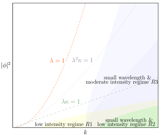
Figure 1: (Color online.) Illustration of the regions in the $k$-$|\phi|^{2}$ plane where the asymptotic regimes R1, R2, R3 are applicable. The dimensionless parameters $\lambda=g|\phi|^{2}/k^{2}$ and $\kappa=k\ell$ define the lines $\lambda=1$, $\lambda^{2}\kappa=1$ and $\lambda\kappa=1$. The dashed (red) line $\lambda=1$ marks the complete breakdown of canonical perturbation theory which requires $\lambda\ll 1$. Regimes R1 and R2 require $\lambda\to 0$ and $\lambda\kappa\to 0$ and thus break down near the dash-dotted (green) line $\lambda\kappa=1$. Regime R3 only requires $\lambda\to 0$ while $\lambda^{n}\kappa$ may not be negligible. Along the dash-dotted (green) line $\lambda\kappa=1$ only first-order perturbation theory gives a non-negligible contribution. Along the dotted line $\lambda^{2}\kappa$ second-order contributions are required.

We may identify three different regimes that are consistent with the canonical perturbation expansion ($\lambda\ll 1$) and may lead to additional simplifications. We explain their range of validity in the following and illustrate it in Fig. 1.

• The low-intensity asymptotic regime $\lambda\to 0$ at fixed $\kappa$ (see illustration in Figure 1). This regime is weak in both the local and the global sense. For the leading nonlinear effects one may expand the oscillatory functions with respect to the small phase shifts (where this leads to a simplification). We will see that this regime allows explicit analytical results that include nonlinear effects to lowest order.

• The short-wavelength globally weak nonlinear asymptotic regime $\kappa\to\infty$ with $\lambda\kappa\to 0$ (see illustration in Figure 1). This regime is a special case of the low-intensity regime which leads to additional simplifications as the dominant nonlinear effects all come from the shift in the nonlinear wave numbers $k_{r}$ and $k_{\eta}$.

• The short-wavelength asymptotic regime with moderately large intensities $\kappa\to\infty$ and $\lambda\to 0$ (see illustration in Figure 1). This regime is weakly nonlinear only in the local but not (necessarily) in the global sense and the intensity is allowed to have moderately large values. As in the globally weak short-wavelength regime, the leading effect is the change of the nonlinear wave numbers $k_{r}$ and $k_{\eta}$ which leads to phase shifts of order $\lambda\kappa$. As these phase shifts may be large, we may not expand the oscillatory terms and the nonlinear effect in the wave function comes in the leading order. If we are only interested in the leading effect, we may neglect all other deformations. In this regime, the equations that describe the stationary states on nonlinear quantum graphs simplify considerably but remain nonlinear.
  A final note on this regime: We have only given the leading shift of the nonlinear wave numbers in (16). This is consistent as long as the intensity is only growing moderately as $\phi_{\mathrm{max}}^{2}=O(k)$ (at fixed $\ell$ and $g$). The regime however allows a larger growth $\phi_{\mathrm{max}}^{2}=o(k^{2})$ but this requires to calculate the nonlinear wave numbers $k_{r}$ and $k_{\eta}$ to higher orders: if $\lambda^{n}\kappa=O(1)$, then we need to calculate $k_{r}$ and $k_{\eta}$ to $n$-th order. While this is possible in principle (see paper1 ), we will confine our discussions to $\lambda^{2}\kappa\ll 1$ (or, equivalently, $\phi_{\mathrm{max}}^{2}\propto k$) with one exception: in our discussion of multi-stability in Sec. III.1 we will consider $\lambda^{2}\kappa=O(1)$ and $\lambda^{3}\kappa\ll 1$.

Apart from finding analytical or numerical solutions in the above mentioned cases, we will also discuss to some extent whether the regimes allow for a quantitative or at least qualitative description of nonlinear effects such as multi-stability of scattering solutions or bifurcations of spectral curves. Our focus here is on how the complexity of the description of example graphs reduces with an appropriate perturbation theory. Therefore, we will usually not give the complete discussion of nonlinear effects that each example graph may deserve. We believe that the methods we present here will be useful for such a detailed analysis in the near future.

I.3 Real solutions

Finally let us state how Eqs. (15) and (16) simplify for essentially real wave functions (real modulo a global complex phase) where the current $I_{\eta}$ vanishes. These equations appear to be singular at $I_{\eta}=0$. The limit $I_{\eta}\to 0$ is, however, well defined and after an appropriate shift of the angle variable $\alpha_{r}(x)$ they reduce to

$$\phi(x)= 2e^{i\eta_{0}}\sqrt{\frac{J_{r}(x)}{k}}\sin\left(\frac{\beta_{r}(x)}{2}\right),$$ (17a)

$$J_{r}(x)= I_{r}\left(1-\frac{gI_{r}}{4k^{3}}\left(4\cos(\alpha_{r}(x))-\cos(2\alpha_{r}(x))\right)+O\left(\lambda^{2}\right)\right),$$ (17b)

$$\beta_{r}(x)= \alpha_{r}(x)+\frac{gI_{r}}{4k^{3}}\left(8\sin(\alpha_{r}(x))-\sin(2\alpha_{r}(x))\right)+O\left(\lambda^{2}\right),$$ (17c)

$$\alpha_{r}(x)= \alpha_{r}(0)+k_{r}x,$$ (17d)

$$k_{r}= 2k\left(1-\frac{3gI_{r}}{2k^{3}}-\frac{51g^{2}I_{r}^{2}}{16k^{6}}+O\left(\lambda^{3}\right)\right)$$ (17e)

where $e^{i\eta_{0}}$ is a fixed global phase of the solution. Note that we have included a term proportional to $g^{2}$ in $k_{r}$. This term can be obtained straight forwardly using canonical perturbation theory to second order in $\lambda$. In most of our discussion, this term will be negligible (apart from Sec. III.1).

II Stationary States in Closed Nonlinear Graphs

Let us now discuss a few examples of closed nonlinear quantum graphs $G$. Exact solutions for the interval and the ring are well-known and are used here to illustrate approximations using canonical perturbation theory – the star and the lasso are added to illustrate how proper graph topologies behave. Our main aim in this section is to describe the spectral curves ${\mu_{n}(N)}$ that give the nonlinear eigenvalues as a function of the $L^{2}$-norm or total intensity

$$N=\sum_{e}\int_{0}^{\ell_{e}}|\phi_{e}(x_{e})|^{2}dx_{e}$$ (18)

which is physically proportional to the number of particles in a Bose-Einstein condensate or the number of photons in an optical setting. In each case we will reduce the problem of solving the generalized nonlinear eigenproblem to a set of (coupled) nonlinear equations with a finite number of unknown variables. Where analytical solutions are available we will give them, but will sometimes have to rely on numerical solutions.

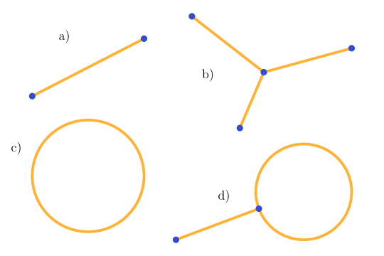
Figure 2: (Color online.) Basic closed graphs analyzed in this paper: (a) an interval, (b) a star graph with three edges, (c) a ring, (d) a tadpole graph (i.e. lasso graph or lollipop graph)

II.1 Nonlinear interval

The stationary NLSE on the interval (as a graph with a single edge connecting two vertices, see Fig. 2a)) $x\in[0,\ell]$ with Dirichlet conditions at both ends $\phi(0)=\phi(\ell)=0$ is straight forward to solve CarrI ; CarrII . In this case the current $I=\mathrm{Im}\ \phi(x)^{*}\phi^{\prime}(x)$ vanishes which leads to the essentially real exact solutions (11) where we set the arbitrary phase $e^{i\eta_{0}}=1$. The Dirichlet condition at $x=0$ implies $x_{0}=0$. The remaining parameters in the solution are the wave number $k\equiv\sqrt{\mu}$ and $\rho_{+}>0$. The latter is a dimensionless measure of the strength of nonlinearity and proportional to the intensity with $\mathrm{max}_{x\in[0,L]}(g|\phi(x)|^{2}/k^{2})=\rho_{+}$ (for $g>0$ it is bounded by $\rho<1$). In order to obey the second Dirichlet condition $\phi(\ell)=0$ as well the wave number $k$ has to be quantized according to

$$k=k_{n}(\rho_{+})\equiv\begin{cases}\frac{2nK\left(\frac{\rho_{+}}{2-\rho_{+}}\right)}{\sqrt{\frac{2-\rho_{+}}{2}}\ell}&\text{if $g>0$}\\ \frac{2nK\left(\frac{\rho_{+}}{2(\rho_{+}+1)}\right)}{\sqrt{\rho_{+}+1}\ell}&\text{if $g<0$.}\end{cases}$$ (19)

for any positive integer $n$. For $\rho_{+}\to 0$ one finds the usual spectrum $k_{n}=\frac{n\pi}{\ell}$ of the linear Schrödinger equation. The total intensity can now be evaluated as

$$N(\rho_{+})=\begin{cases}\frac{2nk_{n}(\rho_{+})\sqrt{4-2\rho_{+}}\left[K\left(\frac{\rho_{+}}{2-\rho_{+}}\right)-E\left(1,\frac{\rho_{+}}{2-\rho_{+}}\right)\right]}{g}&\text{if $g>0$}\\ \frac{2nk_{n}(\rho_{+})(2+\rho_{+})\left[\Pi\left(1,\frac{\rho_{+}}{2(\rho_{+}+1)},\frac{\rho_{+}}{2(\rho_{+}+1)}\right)-K\left(\frac{\rho_{+}}{2(\rho_{+}+1)}\right)\right]}{|g|\sqrt{\rho_{+}+1}}&\text{if $g<0$.}\end{cases}$$ (20)

Equations (19) and (20) implicitly define the nonlinear wave number spectrum $k_{n}(N)$ which is shown in Fig. 3 together with some corresponding wave functions $\phi_{n}(x)$.

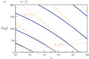
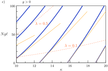
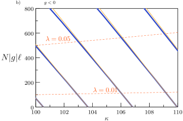
Figure 3: (Color Online.) Spectral curves for the nonlinear interval, the exact curves are shown in blue, the curves derived by canonical perturbation theory in yellow. The curves $\lambda={\rm const.}$ are shown dashed. On the left the regime $g<0$, on the right the regime $g>0$ is considered. The upper panels focus on small values of $\kappa=k\ell$, the lower panels on large values of $\kappa$. (For the purpose of this graph we have defined $\lambda=\frac{|g|N}{k^{2}\ell}$ which is numerically smaller but of the same order compared to the definition in the text.)

With the full solution available for the interval we may use this as a test ground for using the perturbative local solutions that have been developed in Sec. III of paper1 . In first-order perturbation theory the wave function is given by (17). The first Dirichlet condition implies $\alpha_{r}(0)=0$ and we may again set $e^{i\eta_{0}}=1$. The nodal points $x_{n}$ with $\phi(x_{n})=0$ then satisfy $kx_{n}\left(1-\frac{3gI_{r}}{2k^{3}}+O\left(\lambda^{2}\right)\right)=n\pi$. Requiring $\phi(\ell)=0$ thus leads to the condition

$$k=k_{n}(I_{r})=\frac{n\pi}{\ell}\left(1+\frac{3gI_{r}\ell^{3}}{2n^{3}\pi^{3}}+O\left(\lambda^{2}\right)\right)\ .$$ (21)

on the wave number. Note that $\lambda\sim\frac{|g|I_{r}}{k_{n}^{3}}\sim\frac{|g|I_{r}\ell^{3}}{n^{3}}$. The total intensity of the corresponding wave function is

$$N(I_{r})=\frac{2I_{r}\ell}{k_{n}}\left(1+\frac{3gI_{r}}{2k_{n}^{3}}+O\left(\lambda^{2}\right)\right)$$ (22)

which allows us to write $k_{n}$ explicitly in terms of the total intensity

$$k_{n}(N)=\frac{n\pi}{\ell}\left(1+\frac{3gN\ell}{4n^{2}\pi^{2}}+O\left(\lambda^{2}\right)\right)$$ (23)

which is consistent with expanding (19) and (20) for small $\rho_{+}$ and solving for $k_{n}(N)$ including first-order corrections (for either sign of $g$). Note that $\lambda\sim\frac{|g|I_{r}}{k_{n}^{3}}\sim\frac{|g|I_{r}\ell^{3}}{n^{3}}\sim\frac{|g|N\ell}{n^{2}}\sim\frac{|g|N}{k_{n}^{2}\ell}$. Figure 3 compares the exact spectrum and wave functions to the ones obtained using perturbation theory. As expected from the error estimate in (23) the agreement extends to much higher intensities for large values of $\kappa$.
Note that no further assumptions than locally weak nonlinearity (in first-order canonical perturbation theory) have been used to derive (23) which is thus valid in the low-intensity and both small-wavelength regimes introduced in Sec. I.2. The small-wavelength limit corresponds here to $n\to\infty$ where (23) includes the regime R3 where $N$ should grow not faster than $n$. Only the first-order shift in the nonlinear wave number $k_{r}=2k\left(1-\frac{3gI_{r}}{2k^{3}}+O(\lambda^{2})\right)$ enters into the explicit first-order correction term to $k_{n}(I_{r})$ in (21) and $k_{n}(N)$ in (23). For $k_{n}(I_{r})$ higher-order corrections follow directly from higher-order corrections in the nonlinear wave number $k_{r}(I_{r})$. The explicitly given first-order correction (and any higher order corrections) to the intensity $N(I_{r})$ in (22) result from corrections to $k_{r}(I_{r})$ and the deformations of the wave form. This implies that apart from the shift in the nonlinear wave number also the deformations are relevant in higher-order corrections of $k_{n}(N)$.
For consistency let us compare maximal amplitudes in the exact and approximate solutions. One then finds $\rho_{+}+O(\rho_{+}^{2})=\frac{4|g|I_{r}\ell^{3}}{n^{3}\pi^{3}}$ which allows us to express (21) $k_{n}(\rho_{+})=\frac{n\pi}{\ell}\left(1+\mathrm{sgn}(g)\frac{3}{8}\rho_{+}+O(\rho^{2})\right)$ which is indeed the first-order expansion in $\rho_{+}$ of the exact expression (19).
While the shift of the nonlinear wave number and the deformation of the plane wave solution are both affected by the nonlinearity in first-order perturbation theory we see that even for the simplest graph the two effects enter in different ways – and that some leading nonlinear corrections to spectral curves may be found by only referring to the shift.

II.2 Star graphs

A star graph consists of $E$ edges (which we enumerate $e=1,2,\dots,E$) with lengths $\{\ell_{e}\}_{e=1}^{E}$, one vertex of degree $E$ (the center of the graph to which all edges are adjacent) and $E$ vertices of degree one where we assume Dirichlet conditions. For $E=3$ the corresponding graph is depicted in Figure 2b). The ground states of nonlinear star graphs and their stability (with respect to the time-dependent NLSE dynamics) have been the subject of recent research Adami5 ; Adami3 ; Adami6 ; Adami10 ; Adami4 .
We will use the convention that the variable $x_{e}$ on edge $e$ increases towards the center where $x_{e}=\ell_{e}$ while $x_{e}=0$ corresponds to the other end. We will also assume that the coupling constant takes the same constant value $g_{e}\equiv g$ on all edges. As there is no cycle in the graph the current has to vanish everywhere and the wave function ${\phi_{e}(x_{e})}$ may be chosen real.
If some of the edges have rational ratios then we may immediately construct some solutions with a nodal point at the central vertex from the known solutions on the interval. For instance if $\ell_{1}/N_{1}=\ell_{2}/N_{2}=\ell_{0}$ assume that $\phi_{1}(x_{1})$ is a solution of the NLSE on the interval $0\leq x_{1}\leq\ell_{0}$ that we continue smoothly to the edge such that $\phi_{1}(\ell_{1})=0$. Defining $\phi_{2}(x_{2})$ to be the corresponding continuation along edge $e=2$ (that is $\phi_{2}(x_{2}=\ell_{2}-a)=-\phi_{1}(x_{1}=\ell_{1}-a)$) and $\phi_{e}(x_{e})=0$ on all remaining edges we have constructed a solution on the star with a nodal point in the center. Moreover, there will be a corresponding spectral curve $k(N)$ such that the central vertex remains a nodal point for the solutions of this spectral curve. If all edges have rationally independent lengths, then we are not able to build any solutions as easily from the solutions on the interval. There will generally still be some solutions with a nodal point at the center (and a wave function which is supported by a few edges) but these features cannot be expected to be stable along any spectral curve.
Let us now consider the problem of finding spectral curves under the assumption that there is no nodal point at the center. By continuity we can extend this to spectral curves with isolated points with a nodal point at the center. We first reduce the problem of finding exact stationary solutions on a star to a set of nonlinear equations that may be solved numerically in an efficient way. For a given (unperturbed) wave number $k$ the wave function on each edge is given by (11). The Dirichlet conditions $\phi_{e}(0)=0$ imply $x_{0,e}=0$. The remaining parameters $\rho_{+,e}$ and $e^{i\eta_{0,e}}$ have to be found by considering the matching conditions at the center. Let $\phi_{0}=\phi_{e}(\ell_{e})$ be the value of the wave function at the central vertex. By choosing a global phase we assume $\phi_{0}\geq 0$; the wave function is then real and $e^{i\eta_{0,e}}=\pm 1$. The parameters $\rho_{+,e}$ can be found in terms of $\phi_{0}$ by solving the nonlinear equation $|\phi_{e}(\ell)|=\phi_{0}$. This is a nonlinear equation which has in general many solutions $\rho_{+,e}\equiv\rho_{+,e}(\phi_{0};k)$ – for $\phi_{0}\neq 0$ the sign $e^{i\eta_{0,e}}=\pm 1$ then follows from requiring $\phi_{e}(\ell_{e})=\phi_{0}>0$. Choosing one solution branch $\rho_{+,e}=\rho_{+,e}(\phi_{0};k)$ on each edge this leaves $\phi_{0}$ and the wave number $k$ as free parameters. However, we have one more condition to satisfy which is $\sum_{e}\phi_{e}^{\prime}(\ell)=0$; this condition can be compactly written as

$$\sum_{e=1}^{E}\sqrt{1-\frac{\rho_{+,e}}{2}}\frac{\mathrm{cn}\left(\sqrt{1-\frac{\rho_{+,e}}{2}}k\ell_{e},\frac{\rho_{+,e}}{2-\rho_{+,e}}\right)\mathrm{dn}\left(\sqrt{1-\frac{\rho_{+,e}}{2}}k\ell_{e},\frac{\rho_{+,e}}{2-\rho_{+,e}}\right)}{\mathrm{sn}\left(\sqrt{1-\frac{\rho_{+,e}}{2}}k\ell_{e},\frac{\rho_{+,e}}{2-\rho_{+,e}}\right)}= 0 g>0$$ for , and (24a)

$$\sum_{e=1}^{E}\sqrt{1+\rho_{+,e}}\frac{\mathrm{cn}\left(\sqrt{1+\rho_{+,e}}k\ell_{e},\frac{\rho_{+,e}}{2(1+\rho_{+,e})}\right)}{\mathrm{sn}\left(\sqrt{1+\rho_{+,e}}k\ell_{e},\frac{\rho_{+,e}}{2(1+\rho_{+,e})}\right)\mathrm{dn}\left(\sqrt{1+\rho_{+,e}}k\ell_{e},\frac{\rho_{+,e}}{2(1+\rho_{+,e})}\right)}= 0 g<0$$ for . (24b)

We have omitted the explicit dependence of $\rho_{+,e}\equiv\rho_{+,e}(\phi_{0},k)$. We may write the solutions of (24) as spectral curves $k=k_{n}(\phi_{0})$ (where $n$ enumerates disconnected spectral curves). The total intensity $N(\phi_{0})$ is then calculated straight forwardly from the corresponding parameters $\rho_{+,e}$. This implies that we implicitly know $k_{n}(N)$ . Note that as $N\to 0$ all amplitudes $\rho_{e,+}$ have to vanish and the condition (24) reduces to

$$\sum_{e=1}^{E}\mathrm{cot}(k\ell_{e})=0$$ (25)

which is the secular equation for $k$ to be in the spectrum of the corresponding linear star graph where $g=0$ (for rationally independent lengths this gives the complete spectrum).
Numerically, if one point on a spectral curve $k_{n}(\phi_{0})$ is found one may use Newton-Raphson methods to extend this numerically to a finite part of the curve. If one is only interested in spectral curves that connect to the spectrum of the corresponding linear graph it may be numerically more efficient to first solve (25) for the linear spectrum and then extend the curves using Newton-Raphson methods.
While we have reduced the coupled nonlinear problem of finding $E$ parameters $\rho_{+,e}$ (and corresponding signs) to a sequence of $E+1$ relatively benign nonlinear equations that can be solved numerically it remains a formidable task to find all solutions in a given spectral interval (and some restrictions on the maximal local or total intensities).
We now turn to the perturbative solutions for locally weak nonlinearity $g|\phi_{e}|^{2}\ll k^{2}$. The wave function $\phi_{e}(x_{e})$ on each edge $e$ is then given in terms of (17) with $\alpha_{r,e}(0)=0$ and $e^{i\eta_{0,e}}=\mathrm{sgn}\sin(\beta_{r,e}(\ell_{e})/2)$. We need to find a set of $E$ action variables $\{I_{r,e}\}_{e=1}^{E}$ such that the matching conditions at the center are satisfied. The continuity condition $\phi_{e}(\ell_{e})=\phi_{0}$ leads to the nonlinear implicit equation

$$k\phi_{0}^{2}=4J_{r,e}(\ell_{e})\sin^{2}(\beta_{r,e}(\ell_{e})/2)$$ (26)

for $I_{r,e}$. We will later see that the asymptotic regimes R1 and R2 allow us to obtain explicit unique expressions for $I_{r,e}$ in terms of $\phi_{0}^{2}$. In general, (26) may have many solutions which are easy to obtain numerically. Before discussing the asymptotic regimes, let us continue with the general expressions based on first-order perturbation theory. Once the parameters $I_{r,e}$ are found such that (26) is satisfied, we may calculate the total intensity

$$N=\frac{2}{k}\sum_{e=1}^{E}\int_{0}^{\ell_{e}}J_{r,e}(x_{e})\left(1-\cos(\beta_{r,e}(x_{e}))\right)dx_{e}$$ (27)

which at this stage is a function of $\phi_{0}$. The remaining matching condition $\sum_{e}\phi_{e}^{\prime}(\ell_{e})=0$ may be reduced to

$$\sum_{e=1}^{E}\left[\cot\left(\frac{\beta_{r,e}(\ell_{e})}{2}\right)\frac{\beta_{r,e}^{\prime}(\ell_{e})}{2k}+\frac{J_{r,e}^{\prime}(\ell_{e})}{2kJ_{r,e}(\ell_{e})}\right]=0\ .$$ (28)

Here $\beta(\ell_{e})=k_{r,e}\ell_{e}+O\left(\lambda\right)$, $\beta^{\prime}(\ell_{e})=k_{r,e}\left(1+O\left(\lambda\right)\right)$ and $J_{r,e}^{\prime}(\ell_{e})/(2kJ_{r,e}(\ell_{e}))=O\left(\lambda\right)$, so that one obtains

$$\sum_{e=1}^{E}\frac{k_{r,e}}{2k}\cot(k_{r,e}\ell_{e}/2)+O\left(\lambda,\lambda\kappa\right)=0$$ (29)

in leading order, which is consistent with the linear limit where $k_{r,e}\to 2k$. Equations (26), (27), and (28) implicitly define the spectral curves $k_{n}(N)$. While they are simpler than the corresponding exact equations based on Jacobi elliptic functions, they generally remain nonlinear.
Let us now turn to the three asymptotic regimes R1, R2, and R3 where additional simplifications allow for a more explicit form of the solutions. In the low-intensity regime R1 $\lambda\sim g|\phi_{e}|^{2}/k^{2}\propto gI_{r}/k^{3}\to 0$ where $\kappa=k\ell$ is bounded one may expand oscillatory functions such as $\sin(k_{r,e}\ell_{e}/2)$ and consider the leading-order corrections in the continuity condition (26), the total intensity (27), and the quantizations condition (28). In Appendix B we show how these expansions can be used to find spectral curves $k(N)$ in the vicinity of the linear spectrum. If $k_{0}$ is in the spectrum of the linear graph, it satisfies $\sum_{e=1}^{E}\cot(k_{0}\ell_{e})=0$ and the calculation in Appendix B gives the spectral curve $k(N)$ emanating from $k_{0}$ as

$$k(N)=k_{0}\left(1+\frac{gN}{8k_{0}}\left(\frac{\sum_{e=1}^{E}\frac{12k_{0}\ell_{e}-8\sin(2k_{0}\ell_{e})+\sin(4k_{0}\ell_{e})}{\sin^{4}(k_{0}\ell_{e})}}{\sum_{e,e^{\prime}=1}^{E}\frac{k_{0}\ell_{e}}{\sin^{2}(k_{0}\ell_{e})}\frac{2k_{0}\ell_{e^{\prime}}-\sin(2k_{0}\ell_{e^{\prime}})}{\sin^{2}(k_{0}\ell_{e^{\prime}})}}+O\left(\lambda,\lambda^{2}\kappa,\lambda^{2}\kappa^{2}\right)\right)\right)\ .$$ (30)

One may worry about the terms $\sin(k\ell_{e})$ that appear in various denominators and give rise to poles for $k=n\pi/\ell_{e}$. Note that we have already assumed that there is no nodal point in the center $\phi_{0}>0$; moreover, in the low-intensity regime R1 one has $N\to 0$ which implies $\phi_{0}^{2}/\sin^{2}(k\ell_{e})\to 0$ as well.

Next, let us consider the short-wave length regime R2 where $k\to\infty$ with bounded total intensity ($\kappa\to\infty$ and $\lambda\kappa\to 0$ in terms of dimensionless quantitites). In this case, additional simplifications apply (see Appendix B) which result in the spectral curve

$$k(N)=k_{0}\left(1+\frac{gN}{4k_{0}^{2}}\frac{\sum_{e=1}^{E}\frac{3\ell_{e}}{\sin^{4}(k_{0}\ell_{e})}}{\sum_{e,e^{\prime}=1}^{E}\frac{\ell_{e}\ell_{e^{\prime}}}{\sin^{2}(k_{0}\ell_{e})\sin^{2}(k_{0}\ell_{e^{\prime}})}}+O\left(1/\kappa,\lambda/\kappa,\lambda^{2}\kappa\right)\right)$$ (31)

which shows that the slope of the spectral curves decreases fast when $k\to\infty$.

While the regimes R1 and R2 allowed us to express the spectral curves $k(N)$ implicitly as the zeros of an explicit function of $k$ and $N$ the corresponding results may as well have been derived by expanding the exact expressions in terms of elliptic functions in terms of the local amplitudes $\rho_{+,e}$. One strength of the approach based on canonical perturbation theory is that it remains valid even for moderately strong total intensities at small wave lengths. This is the regime R3 where $k\to\infty$ with a total intensity $N\propto k$ that may grow proportional to the wave number (or equivalently, the actions may grow as $I_{r,e}\propto k^{2}$; in terms of dimensionless parameters $\lambda\to 0$, $\kappa\to\infty$ where $\lambda\sim 1/\kappa$). In this case we are not allowed to expand oscillating terms completely. For example, in a term $\sin(k_{r,e}\ell_{e}/2)=\sin(k\ell_{e}-3gI_{r,e}\ell_{e}/2k^{2}+\dots)$ the phase $3gI_{r,e}\ell_{e}/2k^{2}\sim\lambda\kappa$ cannot be considered small. Indeed, these phases give the leading nonlinear effect which is of order unity. Neglecting all other nonlinear effects leads to the set of equations

$$k\phi_{0}^{2}=4I_{r,e}\sin^{2}\left(k\ell_{e}-\frac{3gI_{r,e}\ell_{e}}{2k^{2}}\right)\left(1+O(\lambda,\lambda^{2}\kappa)\right)\qquad\text{for $e=1,\dots,E$;}$$ (32a)

$$N=\frac{2}{k}\sum_{e=1}^{E}I_{r,e}\ell_{e}\left(1+O\left(1/\kappa\right)\right)$$ (32b)

$$\sum_{e=1}^{E}\cot\left(k\ell_{e}-\frac{3gI_{r,e}\ell_{e}}{2k^{2}}\right)\left(1+O(\lambda)\right)=0$$ (32c)

where the neglected term falls off at least as $1/k$ (if the total intensity is allowed to grow $N\propto k$). Note that these equations remain nonlinear and allow in principle for effects such as bifurcation of spectral curves that remain absent in the regimes with globally weak nonlinearity (R1 and R2). For instance Eq. (32a) at fixed $k$ and $\phi_{0}$ has generally more than one solution that is consistent with the range of validity of these equations.

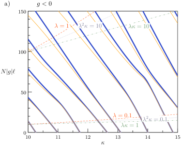
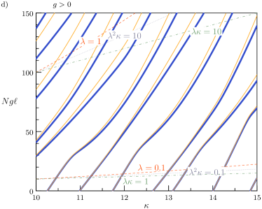
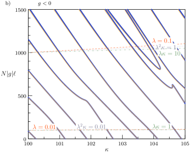
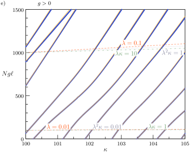
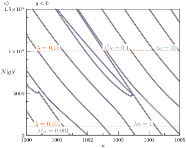
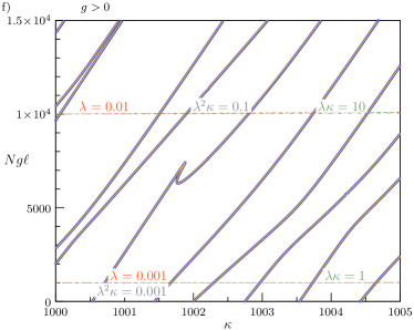
Figure 4: (Color online.) Spectral lines for a star graph with three edges: Exact results (blue curves) are compared with the ones following by canonical perturbation theory (yellow curves). The dashed lines show the curves $\lambda={\rm const.}$, $\lambda\kappa={\rm const.}$ and $\lambda\kappa^{2}={\rm const.}$. (For the purpose of this graph we have defined $\lambda=\frac{|g|N}{k^{2}\ell}$ which is numerically different but of the same order compared to the definition in the text.)

Indeed, one can find bifurcations of spectral curves in the exact spectral curves and these are well described by the asymptotic approximation (32) in the short-wave length regime R3. This can be seen in Fig. 4 where we compare the spectral curves obtained from exact solutions with approximative solutions based on (32). The agreement of the curves clearly improves with increasing wave number $k$ and extends to higher total intensities $N$ as $k$ is increased. We have found some new spectral curves appearing at higher intensities which are not connected to the linear spectrum at $N=0$. We do not want to suggest that we have found all spectral curves in the shown intervals. The spectral curves that extend to the linear spectrum were found using a Newton Raphson method by deforming the (easily available) linear solution. We would like to note that the computations using the asymptotic approximation (32) were considerably quicker. Indeed, the bifurcations where new spectral curves appear at larger intensities have usually first to be found using the asymptotic equations before (which could then be used as a starting point to find the exact ones). In a very different regime (negative chemical potential), bifurcations in the ground state have been analyzed in Adami6 .

II.3 The ring

Next, let us consider a ring of total length $\ell$ illustrated in Fig. 2(c) where the spectrum of the linear case is just the collection of eigenvalues $\mu_{n}=k_{n}^{2}=\frac{4\pi^{2}n^{2}}{\ell^{2}}$ for $n=0,1,\dots$ (we will always assume $k_{n}\geq 0$). Here, $n=0$ corresponds to the constant function and eigenvalues $n\geq 1$ are double degenerate with corresponding eigenfunctions of the form $\phi(x)=Ae^{ik_{n}x}+Be^{-ik_{n}x}$ such that the intensity $|\phi(x)|^{2}$ is constant for $A=0$ or $B=0$ and has discrete nodal points for $|A|=|B|>0$. The exact solutions in the nonlinear case have been studied in detail before in terms of Jacobi elliptic equations for repulsive CarrI and attractive nonlinearity CarrII . Here, we want to give a short overview how the equations simplify for locally weak nonlinearity where first-order canonical perturbation theory applies. The main new feature compared to the interval or star graphs is that the wave functions may be genuinely complex valued. This is accompanied by the fact that there are now two distinct periodicities described by the nonlinear wave numbers $k_{r}$ and $k_{\eta}$. In the linear limit, their ratio takes a unique value $k_{r}/k_{\eta}=2$ and we will see that in the nonlinear case this ratio can take other (rational) values.
Let us start with stating the conditions for an exact solution $\phi(x)=r(x)e^{i\eta(x)}$ which is locally given by (6) and (8) with $x_{0}=0$ (by choice of origin) and with the periodicity condition $\phi(x)=\phi(x+\ell)$ for all $x$. This implies

$$r(x+\ell)= r(x),$$ (33a)

$$\varphi(x+\ell)= \varphi(x)\;\;\mathrm{mod}\ 2\pi.$$ (33b)

The solutions (6) and (8) depend on two parameters $\rho_{\pm}$ such that $\rho_{-}\leq\frac{|g|r(x)^{2}}{k^{2}}\leq\rho_{+}$. For a given value of the wave number $k$ the two conditions (33) can be satisfied for a discrete set of values $(\rho_{+,n}(k),\rho_{-,n}(k))$. With the total intensity $N=\int_{0}^{\ell}r(x)^{2}dx$ each of the solutions $(\rho_{+,n}(k),\rho_{-,n}(k))$ then defines a spectral curve $N_{n}(k)$.
We want to discuss these curves using canonical perturbation theory to first order where the wave function is given by Equations (14) and (15) (with $\alpha_{r}(0)=0=\alpha_{\eta}(0)$ by choice of origin and global phase). These solutions depend on the two action variables $I_{r}\geq 0$ and $I_{\eta}$ which need to be determined through conditions (33). Complex conjugation of a solution gives a new solution that is given by replacing $I_{\eta}\mapsto-I_{\eta}$. We may thus confine our discussion to non-negative values $I_{\eta}\geq 0$. For $I_{r}>0$ the periodicity conditions imply

$$k_{r}= 2k\left(1-\frac{3g}{2k^{3}}I_{r}-\frac{3g}{4k^{3}}I_{\eta}+O\left(\lambda^{2}\right)\right)=\frac{2\pi(2n-m\ \mathrm{sgn}(g))}{\ell},$$ (34a)

$$k_{\eta}= k\left(1-\frac{3g}{2k^{3}}I_{r}-\frac{g}{2k^{3}}I_{\eta}+O\left(\lambda^{2}\right)\right)=\frac{2\pi n}{\ell},$$ (34b)

where $n$ and $m$ are integers. Here $n=1,2,\dots$ may take any positive value which is obvious from the second equation. We will see later that $m=0,1,2,\dots$ takes non-negative values and this is the reason for writing $2n-m\ \mathrm{sgn}(g)$ in the first condition. If $I_{r}=0$ the intensity is constant and only the second condition applies which then reduces to

$$\left.k_{\eta}\right|_{I_{r}=0}=k\left(1-\frac{gI_{\eta}}{2k^{3}}+O\left(\lambda^{2}\right)\right)=\frac{2\pi n}{\ell}\ .$$ (35)

Note that in this case the integer $m$ is not defined. With $N=\frac{I_{\eta}\ell}{k}\left(1+O(\lambda)\right)$ one obtains a spectral curve

$$k_{n}(N)=\frac{2\pi n}{\ell}\left(1+\frac{gN\ell}{8\pi^{2}n^{2}}+O\left(\lambda^{2}\right)\right)\ .$$ (36)

These spectral curves connect to the linear spectrum as $k_{n}(0)=\frac{2\pi n}{\ell}$.
Setting $m=0$ in (34) leads to another set of spectral curves that connect to the linear spectrum. In this case $I_{\eta}=0$ and we have an essentially real wave function (modulo choice of a global phase) with $2n$ nodal points such that the problem reduces to the nonlinear interval of length $\ell/2$. The corresponding spectral curves are given by

$$k_{n,0}(N)=\frac{2\pi n}{\ell}\left(1+\frac{3gN\ell}{16\pi^{2}n^{2}}+O\left(\lambda^{2}\right)\right),$$ (37)

where $N=\frac{2I_{r}\ell}{k}\left(1+O(\lambda)\right)$. Note that so far the discussion has been consistent with the globally weak asymptotic regimes R1 and R2 as well as the short-wave length regime with moderate intensities R3. Let us now discuss the case $m>0$. First, note that eliminating $n$ from (34) gives

$$m=\frac{|g|\ell}{4\pi k^{2}}I_{\eta}\left(1+O(\lambda)\right),$$ (38)

which is manifestly non-negative (as we confined the discussion to $I_{\eta}\geq 0$ without loss of generality), so that $m=0,1,\dots$ is a non-negative integer as stated above. Moreover, if we want to have $m>0$ then (38) shows that this is not consistent with globally weak nonlinearity (regimes R1 and R2) where the right-hand side becomes arbitrarily small in the asymptotic limit. On the other hand the short-wave length regime R3 with modestly large intensities allows for the right-hand side to be of order unity (as $I_{\eta}$ is allowed to take values $O(k^{2})$). The rest of the discussion will be confined to this regime where the $I_{\eta}$ and $I_{r}$ are of order $O(k^{2})$ and $n\propto k\ell\gg 1$ (so $n=O(k)$) while $m\ll n$ takes small integer values ($m=O(k^{0})$). Solving (34) for the action variables gives

$$I_{\eta}= \frac{4\pi mk^{2}}{|g|\ell}\left(1+O\left(\lambda\right)\right)$$ (39a)

$$I_{r}= \frac{2k^{2}}{3g\ell}\left(k\ell-2\pi\left(n+\frac{g}{|g|}m\right)+O\left(\lambda\right)\right)\ .$$ (39b)

Note that the second equation implies that $I_{r}$ changes sign at $\kappa=k\ell=2\pi\left(n+\frac{g}{|g|}m\right)+O(\lambda)$. As $I_{r}$ is manifestly positive this defines an endpoint of a spectral curve where $I_{\eta}=\frac{16\pi^{3}mn^{2}}{|g|\ell^{3}}\left(1+O(\lambda)\right)>0$ is not vanishing at the same time. With $N=\frac{(2I_{r}+I_{\eta})\ell}{k}\left(1+O(\lambda)\right)$ the corresponding spectral curve

$$k_{n,m}(N)=\frac{2\pi n}{\ell}\left(1-\frac{g}{|g|}\frac{m}{2n}+\frac{3g\ell}{16\pi^{2}n^{2}}N\right)+O(\lambda,\kappa\lambda^{2})\quad\text{for $N>\frac{8\pi^{2}mn}{|g|\ell}$ }$$ (40)

does not connect directly to the linear spectrum. Rather it bifurcates from the spectral curve $k_{n}(N)$ given by (36) at a finite total intensity $N\approx\frac{8\pi^{2}mn}{|g|\ell}$. This bifurcation scenario is depicted in Figure 5.

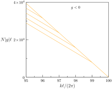
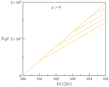
Figure 5: (Color online.) Approximative bifurcation scenario for spectral curves on a ring graph. The spectral curve $k_{n}(N)$ (see Eq. (36)) is shown for $n=100$ together with the spectral curves $k_{n,m}$ (see Eq. (40)) that bifurcate above a critical intensity. The approximations are valid in the high wave number asymptotic regime R3.

II.4 The tadpole (aka lasso aka lollipop) graph

The tadpole graph consists of a ring graph of length $\ell_{1}$ to which one dangling edge of length $\ell_{2}$ is attached at one end (see Fig. 2(d)). We choose the coordinates on the ring such that $-\ell_{1}/2\leq x_{1}\leq\ell_{1}/2$ where $x_{1}=-\ell_{1}/2$ (and equivalently $x_{1}=\ell_{1}/2$) is the position of the vertex where the dangling edge is attached. The coordinate on the dangling edge will be chosen such that $0\leq x_{2}\leq\ell_{2}$ with $x_{2}=0$ for the vertex of degree one and $x_{2}=\ell_{2}$ for the vertex that connects to the ring. We assume Dirichlet boundary conditions $\phi_{2}(0)=0$ at the dangling vertex and standard matching conditions

$$\phi_{2}(\ell_{2})=\phi_{1}(-\ell_{1}/2)=\phi_{1}(\ell_{1}/2)$$ (41a)

$$\phi_{1}^{\prime}(-\ell_{1}/2)-\phi_{1}^{\prime}(\ell_{1}/2)-\phi_{2}^{\prime}(\ell_{2})=0$$ (41b)

at the vertex on the ring. One may observe that the real solutions of the ring considered in Sec. II.3 can be extended to a solution on the tadpole: if one of the nodal points is on the vertex and we set $\phi_{2}(x_{2})\equiv 0$, then all matching conditions are satisfied. If we try to extend the (non-trivially) complex solutions on the ring (with a finite current) to the tadpole then, due to the lack of nodal points, this can only be done with a non-vanishing solution on the dangling edge such that $\phi_{2}^{\prime}(\ell_{2})=0$. This can in general not be satisfied at the same time as continuity. However, there is also the additional rotational freedom of solutions on the ring – so the problem of extending a ring solution to the tadpole reduces to the condition $\phi_{2}^{\prime}(\ell_{2})=0$ where $\phi_{2}(\ell_{2})\in{|\phi_{1}(x_{1})|:0\leq x_{1}\leq\ell_{1}}$. While this may not work for arbitrary ring solutions one expects that at least some (non-trivially) complex nonlinear ring solutions can be extended to the tadpole for any values of the lengths $\ell_{1}$ and $\ell_{2}$. Interestingly, in the linear case ($g=0$) this is generally not the case because solutions do not change with the overall scaling.
In the linear case, complex solutions with a finite current around the ring only exist for wave numbers $k$ that satisfy $\cos(k\ell_{2})=0$ and $e^{ik\ell_{1}}=1$ at the same time. This in turn implies that the quotient of the two lengths is rational $\frac{\ell_{2}}{\ell_{1}}=\frac{2n_{2}+1}{4n_{1}}$ (where $n_{1}>0$ and $n_{2}\geq 0$ are integers). The linear wave number spectrum is then discrete and non-degenerate. One half of the spectrum $k=n\frac{2\pi}{\ell_{1}}$ for positive integers $n$ corresponds to wave functions

$$\phi_{1}(x_{1})=\sin(k(x_{1}+\ell_{1}/2))\quad\text{and}\quad\phi_{2}(x_{2})\equiv 0$$ (42)

on the ring with a nodal point on the vertex while the other half can only be given implicitly as the zeros of the equation

$$\tan\left(k\ell_{2}\right)\tan\left(k\ell_{1}/2\right)=\frac{1}{2}\ .$$ (43)

The wave functions corresponding to the latter solutions are of the form

$$\phi_{1}(x_{1})=\frac{\sin(k\ell_{2})}{\cos(k\ell_{1}/2)}\cos(kx_{1})\quad\text{and}\quad\phi_{2}(x_{2})=\sin(kx_{2})$$ (44)

which have a non-vanishing value $\sin(k\ell_{2})\neq 0$ at the vertex which follows from condition (43) and the assumption that $\ell_{1}/\ell_{2}$ is irrational.

In the nonlinear case the exact solutions were classified in Finco and their stability and bifurcations were studied in Noja . We will now establish a few complex solutions using canonical perturbation theory in the generic case where $\ell_{1}/\ell_{2}$ is irrational. In the previous sections we have seen that the asymptotic low-intensity regimes R1 and the globally weakly nonlinear short wave length regime R2 describe how nonlinear solutions connect to the linear solutions while not being able to describe any bifurcations. The same applies in the present context, so we immediately consider the short wave length asymptotic regime R3 and try to find solutions of the form

$$\phi_{1}(x_{1})= \frac{e^{ik_{\eta,1}x_{1}}}{\sqrt{k}}\left(\sqrt{I_{r,1}+I_{\eta,1}}\pm\sqrt{I_{r,1}}e^{-ik_{r,1}x_{1}}\right)\left(1+{O}\left(\lambda\right)\right)$$ (45a)

$$\phi_{2}(x_{2})= 2e^{i\beta}\sqrt{\frac{I_{r,2}}{k}}\sin\left(k_{r,2}x_{2}/2\right)\left(1+{O}\left(\lambda\right)\right)$$ (45b)

where the form of $\phi_{1}(x_{1})$ ensures that $|\phi_{1}(-\ell_{1}/2)|=|\phi_{1}(\ell_{1}/2)|$. We have also chosen $I_{\eta_{1}}\geq 0$ such that complex solutions have a current along the ring in increasing direction of $x_{1}$. By complex conjugation one then finds a new solution with opposite current (i.e. the corresponding solution with negative $I_{\eta,1}$).
Before considering how some complex solutions can be described let us first consider the appreciable simpler case of real solutions where $I_{\eta,1}=0$ and $k_{\eta,1}=k_{r,1}/2$. In that case the two choices of the sign in $\phi_{1}(x_{1})$ lead to

$$\phi_{1}(x_{1})=2\sqrt{\frac{I_{r,1}}{k}}\begin{cases}i\sin\left(k_{\eta,1}x_{1}\right)\left(1+{O}\left(\lambda\right)\right)\\ \cos\left(k_{\eta,1}x_{1}\right)\left(1+{O}\left(\lambda\right)\right)\end{cases}$$ (46)

It is straight forward to see from $\phi_{1}(-\ell_{1}/2)=\phi_{1}(\ell_{1}/2)$ that the sine solutions must have a nodal point at the vertex which implies $k_{\eta,1}=\frac{2\pi n}{\ell_{1}}$ and that the wave function on the dangling bond is identically zero $\phi_{2}(x_{2})\equiv 0$. We identify these solutions as the nonlinear solutions on the ring. The corresponding spectral curves are given by (37) and connect to the corresponding part of the linear spectrum. Choosing the cosine in (46) leads to the condition

$$\tan\left(\frac{k_{\eta,1}\ell_{1}}{2}\right)\tan\left(\frac{k_{r,2}\ell_{2}}{2}\right)= \frac{k_{r,2}}{4k_{\eta,1}}\left(1+{O}\left(\lambda\right)\right)$$ (47a)

$$I_{r,1}\cos^{2}\left(\frac{k_{\eta,1}\ell_{1}}{2}\right)= I_{r,2}\sin^{2}\left(\frac{k_{r,2}\ell_{2}}{2}\right)\left(1+{O}\left(\lambda\right)\right)$$ (47b)

$$N= \frac{2I_{r,1}\ell_{1}}{k}\left(1+{O}\left(1/\kappa\right)\right)+\frac{2I_{r,2}\ell_{2}}{k}\left(1+{O}\left(1/\kappa\right)\right)$$ (47c)

which together define spectral curves $k(N)$. In the limit $N\to 0$ we have $k_{\eta,1}\to k$ and $k_{r,2}\to 2k$ and the condition (47a) becomes the implicit equation (43) for the corresponding linear spectrum. Altogether we found a clear correspondence between the real nonlinear solutions and corresponding linear solutions of the tadpole graph.
In addition to the real solutions there may be a large number of complex solutions. With the canonical perturbation approach we have reduced the problem of finding all complex solutions to a finite set of non-linear conditions (41) that can in general be solved numerically. In the present setting, we restrict ourselves to establish the existence of some complex solutions analytically. Let us consider only the leading behavior and look for solutions that satisfy the additional condition $I_{r,1}=0$. This condition implies that the intensity on the ring is constant, $|\phi_{1}(x_{1})|^{2}=\frac{I_{\eta,1}}{k}\left(1+O(\lambda)\right)$. In this case the matching condition $\phi_{1}(\ell_{1}/2)=\phi_{1}(-\ell_{1}/2)$ implies

$$k_{\eta,1}\ell_{1}\equiv k\ell_{1}\left(1-\frac{g}{2k^{3}}I_{\eta,1}\right)+O\left(\lambda,\lambda^{2}\kappa\right)=n_{1}\pi$$ (48)

for some integer $n_{1}>0$. In this case $\phi_{1}^{\prime}(\ell_{1}/2)=\phi_{1}^{\prime}(-\ell_{1}/2)$ which reduces the matching condition (41b) to $\phi_{2}^{\prime}(\ell_{2})=0$ or

$$k_{r,2}\ell_{2}\equiv 2k\ell_{2}\left(1-\frac{3g}{2k^{3}}I_{r,2}\right)+O\left(\lambda,\lambda^{2}\kappa\right)=(2n_{2}-1)\pi$$ (49)

for a positive integer $n_{2}>0$. The remaining matching conditions $\phi_{2}(\ell_{2})=\phi_{1}({-\ell_{1}/2})$ just implies $4I_{r,2}=I_{\eta,1}$. We may replace one of the two conditions (48) and (49) by the quotient

$$\frac{(2n_{2}-1)\ell_{1}}{2\ell_{2}n_{1}}=1+\frac{g}{2k^{3}}I_{r,2}+O\left(\lambda/\kappa,\lambda^{2}\right)\ .$$ (50)

This is a single condition for the combination $\frac{g}{2k^{3}}I_{r,2}$. If it is satisfied the individual conditions (48) and (49) are straight forwardly satisfied by considering $k$ and $I_{r,2}$ independently. So let us show that (50) can indeed be satisfied in the short wave length regime. In this regime one may choose $n_{1}$ and $n_{2}$ large such that the ratio $\frac{2n_{2}-1}{2n_{1}}$ is a rational approximant to (the irrational number) $\ell_{2}/\ell_{1}$ or $\frac{(2n_{2}-1)\ell_{1}}{2\ell_{2}n_{1}}=1+\delta$ where $\delta$ may be positive or negative and arbitrarily small. Choosing $\frac{g}{2k^{3}}I_{r,2}=\delta$ then satisfies the condition (in leading order).
We see that a relatively simple graph such as the tadpole already has a rich set of solutions. Within canonical perturbation theory we have shown straight forwardly that there exist solutions to the nonlinear tadpole which are not just deformations of the solutions of the corresponding linear problem. It would certainly be interesting to study the full bifurcation scenario of the spectral curves $k(N)$ in this case using canonical perturbation theory; in this paper we confine ourselves to initial steps in a variety of simple graphs and thus leave this as an open problem for later investigation.

III Wave Scattering from Nonlinear Graph Structures

In this section we discuss stationary scattering from nonlinear graphs. We will consider a few simple graphs with some nonlinear bonds and linear leads. We will fix incoming wave amplitudes on the leads and be interested in reflection and transmission amplitudes through the nonlinear graph. In the linear setting these amplitudes are described by a scattering matrix Kottos1 ; Kottos2 . Scattering through nonlinear graphs was studied previously by different methods in Adami ; Sobirov ; Holmer ; Uecker . We will use canonical perturbation theory to show how the nonlinear setting connects to the known linear description at low intensities and also discuss how multi-stability as a proper nonlinear effect can be described in this framework. As before we do not aim at a complete description of each example graph.

III.1 Nonlinear interval connected to a single lead

We consider a nonlinear interval of length $\ell$ with Dirichlet boundary condition at $x=0$ and a linear interval coupled at $x=\ell$ (see Fig. 6a)).

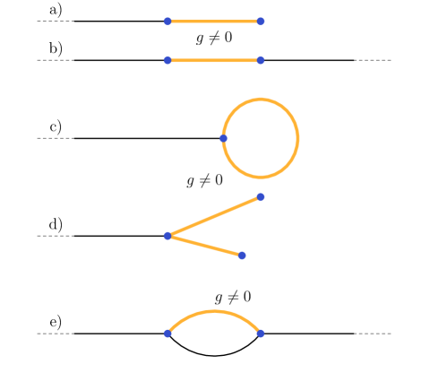
Figure 6: (Color online.) Basic open graphs considered in the main text: (a) one linear lead, connected to a nonlinear interval, (b) a nonlinear interval connected to two linear leads on both ends, (c) a nonlinear ring connected to a linear lead, (d) a Y-structure with two nonlinear bonds and a linear lead meeting in one vertex; one may also refer to this as scattering from a nonlinear 2-star, or a T-structure (aligning the two bonds); (e) two bonds (one linear one non-linear) creating a cycle and two linear leads.

It is ideal for testing the power of the canonical perturbation theory for a scattering setup. We write the wave function as

$$\phi(x)=\begin{cases}\phi_{\mathrm{NL}}(x)e^{i\delta/2}&\text{for $x<\ell$,}\\ \sqrt{\frac{I_{L}}{k}}(e^{-ikx}+e^{i\delta}e^{ikx})&\text{for $x>\ell$}\end{cases}$$ (51)

where $\phi_{\mathrm{NL}}(x)$ is a real nonlinear solution given in equation (11) (with $x_{0}=0$ to satisfy the Dirichlet condition and $\eta_{0}=0$). The parameter $I_{L}$ in (51) is the current of the incoming wave. The reflected wave contains an additional scattering amplitude $e^{i\delta}$. In an experiment one sets the current $I_{L}$ and the wave number $k$ and measures the scattering phase $\delta$ as a function of $k$ and $I_{L}$. In the linear case the scattering phase is $\delta=\pi$ (or $e^{i\delta}=-1$) which follows from the Dirichlet condition at $x=0$. At a given wave number $k$ the nonlinear wave function $\phi_{\mathrm{NL}}(x)$ depends on the single parameter $\rho_{+}$. If we fix $\rho_{+}$ we may determine $I_{L}$ and $\delta$ from the continuity of the wave function and its derivative at $x=\ell$. This is equivalent to considering the point $x=\ell$ as a vertex on graph with two edges (a finite bond and an infinite lead) with the standard matching conditions described in Section I.1.2. This leads to the exact and unique relation between $I_{L}$ and $\rho_{+}$

$$I_{L}(\rho_{+})= \frac{k^{2}\phi_{\mathrm{NL}}(\ell)^{2}+\phi_{\mathrm{NL}}^{\prime}(\ell)^{2}}{4k}$$ (52)

$$= \begin{cases}\frac{k^{3}\rho_{+}}{4g}\left[\mathrm{sn}^{2}\left(k\sqrt{\frac{(2-\rho_{+})}{2}}\ell,\frac{\rho_{+}}{2-\rho_{+}}\right)+\left(1-\frac{\rho_{+}}{2}\right)\mathrm{cn}^{2}\left(k\sqrt{\frac{(2-\rho_{+})}{2}}\ell,\frac{\rho_{+}}{2-\rho_{+}}\right)\mathrm{dn}^{2}\left(k\sqrt{\frac{(1-\rho_{+})}{2}}\ell,\frac{\rho_{+}}{2-\rho_{+}}\right)\right]&\text{if $g>0$}\\ \frac{k^{3}}{|g|}\frac{\rho_{+}(2+\rho_{+})}{8(1+\rho_{+})}\left[\frac{\mathrm{sn}^{2}\left(k\sqrt{1+\rho_{+}}\ell,\frac{\rho_{+}}{2(1+\rho_{+})}\right)}{\mathrm{dn}^{2}\left(k\sqrt{1+\rho_{+}}\ell,\frac{\rho_{+}}{2(1+\rho_{+})}\right)}+(1+\rho_{+})\frac{\mathrm{cn}^{2}\left(k\sqrt{1+\rho_{+}}\ell,\frac{\rho_{+}}{2(1+\rho_{+})}\right)}{\mathrm{dn}^{4}\left(k\sqrt{1+\rho_{+}}\ell,\frac{\rho_{+}}{2(1+\rho_{+})}\right)}\right].&\text{if $g<0$.}\end{cases}$$ (53)

The scattering amplitude may generally be expressed as

$$e^{i\delta}=-e^{-i2k\ell}\frac{\phi_{\mathrm{NL}}^{\prime}(\ell)+ik\phi_{\mathrm{NL}}(\ell)}{\phi_{\mathrm{NL}}^{\prime}(\ell)-ik\phi_{\mathrm{NL}}(\ell)}$$ (54)

which leads to the phase shift

$$\delta(\rho_{+})=\begin{cases}\mathrm{arg}\left(e^{i(\pi-2k\ell)}\frac{\sqrt{\frac{(2-\rho_{+})}{2}}\mathrm{cn}\left(k\sqrt{\frac{(2-\rho_{+})}{2}}\ell,\frac{\rho_{+}}{2-\rho_{+}}\right)\mathrm{dn}\left(k\sqrt{\frac{(2-\rho_{+})}{2}}\ell,\frac{\rho_{+}}{2-\rho_{+}}\right)+i\mathrm{sn}\left(k\sqrt{\frac{(2-\rho_{+})}{2}}\ell,\frac{\rho_{+}}{2-\rho_{+}}\right)}{\sqrt{\frac{(2-\rho_{+})}{2}}\mathrm{cn}\left(k\sqrt{\frac{(2-\rho_{+})}{2}}\ell,\frac{\rho_{+}}{2-\rho_{+}}\right)\mathrm{dn}\left(k\sqrt{\frac{(2-\rho_{+})}{2}}\ell,\frac{\rho_{+}}{2-\rho_{+}}\right)-i\mathrm{sn}\left(k\sqrt{\frac{(2-\rho_{+})}{2}}\ell,\frac{\rho_{+}}{2-\rho_{+}}\right)}\right)&\text{if $g>0$;}\\ \mathrm{arg}\left(e^{i(2k\ell-\pi)}\frac{\sqrt{1+\rho_{+}}\mathrm{cn}\left(k\sqrt{1+\rho_{+}}\ell,\frac{\rho_{+}}{2(1+\rho_{+})}\right)+i\mathrm{sn}\left(k\sqrt{1+\rho_{+}}\ell,\frac{\rho_{+}}{2(1+\rho_{+})}\right)\mathrm{dn}\left(k\sqrt{1+\rho_{+}}\ell,\frac{\rho_{+}}{2(1+\rho_{+})}\right)}{\sqrt{1+\rho_{+}}\mathrm{cn}\left(k\sqrt{1+\rho_{+}}\ell,\frac{\rho_{+}}{2(1+\rho_{+})}\right)-i\mathrm{sn}\left(k\sqrt{1+\rho_{+}}\ell,\frac{\rho_{+}}{2(1+\rho_{+})}\right)\mathrm{dn}\left(k\sqrt{1+\rho_{+}}\ell,\frac{\rho_{+}}{2(1+\rho_{+})}\right)}\right)&\text{if $g<0$.}\end{cases}$$ (55)

Implicitly this defines the scattering phase $\delta$ as a function of the incoming flow $I_{L}$. It is well-known that multi-stability and related hysteresis effects occur already in the most basic nonlinear scattering systems such as the one considered here. In the present context, hysteresis physically implies that the outcome of an experiment where $I_{L}$ and $k$ are given and $\delta$ is measured depends on the history of the experiment which selects one (stable) branch out of many. Numerically this is indeed seen straight forwardly. This is shown in Fig. 7 where $\delta(I_{L})$ is depicted for some values of $k$. As can be seen, there is a critical value $I_{L}^{\mathrm{(c)}}$ such that multi-stability sets in above $I_{L}>I_{L}^{\mathrm{(c)}}$ and this value increases with $k$.

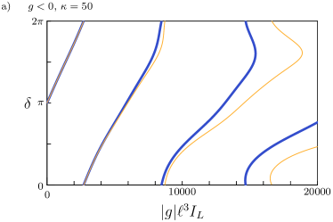
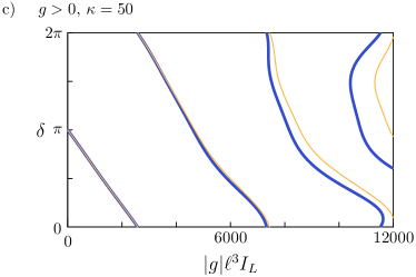
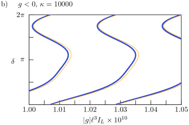
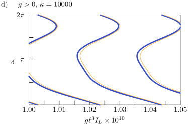
Figure 7: (Color online.) Scattering phase for an interval connected to one lead as a function of $g\ell^{3}I_{L}$. The blue curves depict the exact results whereas the results based on canonical perturbation theory are shown as yellow curves. The flow is plotted in natural dimensionless units as $|g|\ell^{3}I_{L}$.

In the remainder of this chapter we want to use canonical perturbation theory in order to approximate the nonlinear effects in the scattering phase and to give an analytical estimate how the critical flow $I_{L}^{\mathrm{(c)}}$ increases with $k$. The wave function $\phi_{\mathrm{NL}}(x)$ is then given by Eq. (17) (with $\alpha_{r}(0)=0$ and $\eta_{0}=0$). The scattering amplitude can then be expressed as

$$e^{i\delta}=-e^{i\left(\beta_{r}(\ell)-2k\ell\right)}\frac{2kJ_{r}(\ell)+e^{-i\beta_{r}(\ell)/2}\left[(\beta^{\prime}_{r}(\ell)-2k)J_{r}(\ell)\cos(\beta_{r}(\ell)/2)+J^{\prime}_{r}(\ell)\sin(\beta_{r}(\ell)/2)\right]}{2kJ_{r}(\ell)+e^{i\beta_{r}(\ell)/2}\left[(\beta^{\prime}_{r}(\ell)-2k)J_{r}(\ell)\cos(\beta_{r}(\ell)/2)+J^{\prime}_{r}(\ell)\sin(\beta_{r}(\ell)/2)\right]}$$ (56)

and the incoming flow as

$$I_{L}=J_{r}(\ell)\sin^{2}\left(\frac{\beta_{r}(\ell)}{2}\right)+\frac{1}{4k^{2}}\left[\frac{J_{r}^{\prime}(\ell)}{\sqrt{J_{r}(\ell)}}\sin\left(\frac{\beta_{r}(\ell)}{2}\right)+\sqrt{J_{r}(\ell)}\beta_{r}^{\prime}(\ell)\cos\left(\frac{\beta_{r}(\ell)}{2}\right)\right]^{2}$$ (57)

The low-intensity regimes R1 and R2 do not allow for multi-stability because the asymptotic limit is not compatible with describing nonlinear effects above a critical value.
Let us now turn to the short-wavelength regime $R3$. In this regime, $\lambda=\frac{g|\phi|^{2}}{k^{2}}\to 0$ and $\kappa=k\ell\to\infty$. In all previous examples we could capture interesting nonlinear effects by only considering the leading order corrections of order $\lambda\kappa$ to the phase while neglecting contributions $O(\lambda^{2}\kappa)$ to the phase and $O(\lambda)$ (relative to the leading term) to the amplitude. We will show that the critical value $I_{L}^{\mathrm{(c)}}$ scales like $k^{2.5}$ which implies that $\lambda^{2}\kappa$ cannot be neglected as $k\to\infty$. The detailed calculation can then only be performed consistently if one also keeps corrections $O(\lambda)$ to the amplitude. Using (56) and (57) one then obtains

$$I_{L}(I_{r})=I_{r}\left[1+\frac{gI_{r}}{4k^{3}}\left(\cos(2\alpha)-4\cos(\alpha)\right)+O(\lambda^{2})\right]$$ (58)

and

$$\delta(I_{r})=\pi+\alpha-2k\ell+\frac{gI_{r}}{k^{3}}\left(2\sin(\alpha)-\frac{1}{4}\sin(2\alpha)\right)+O(\lambda^{2})$$ (59)

where

$$\alpha=2k\ell\left(1-\frac{3gI_{r}}{2k^{3}}-\frac{51g^{2}I_{r}^{2}}{16k^{6}}+O(\lambda^{3})\right)\ .$$ (60)

Figure 7 shows the scattering phase $\delta(I_{L})$ by numerically solving (58) and (59) and compares it to the numerical solution of the exact equations. As can be seen multi-stability can be accurately described numerically.
The expressions can also be used for analytical estimates. A unique function is only obtained if the function (58) is a monotonic function of $I_{r}$. If $I_{r}^{\mathrm{(c)}}$ is the smallest value such that $\frac{dI_{L}}{dI_{r}}=0$ then multi-stability sets in for $I_{r}>I_{r}^{\mathrm{(c)}}$, and since the incoming flow $I_{L}$ is equal to $I_{r}$ to leading order we get multi-stability for incoming flows $I_{L}>I_{L}^{\mathrm{(c)}}=I_{r}^{\mathrm{(c)}}$. This value can be estimated straight forwardly from (58) by taking the derivative

$$\frac{dI_{L}}{dI_{r}}=1+\frac{3g^{2}I_{r}^{2}\ell}{2k^{5}}\left(\sin(2\alpha)-2\sin(\alpha)\right)+O\left(\lambda,\lambda^{3}\kappa\right),$$ (61)

which shows that the derivative can only vanish if $\frac{g^{2}I_{r}^{2}\ell}{k^{5}}$ is of order unity which gives the estimate

$$I_{L}^{\mathrm{(c)}}=\frac{k^{5/2}}{|g|\ell^{1/2}}.$$ (62)

Fig. 8 compares this estimate $I_{L}^{\mathrm{(c)}}$ to the numerically obtained critical value using the exact equations.

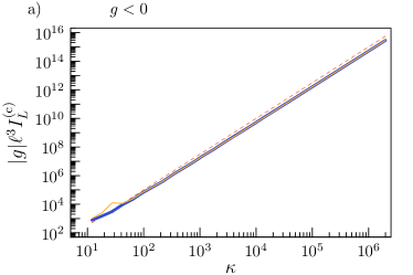
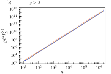
Figure 8: (Color online.) Double logarithmic plot of the critical incoming flow $I_{L}^{\mathrm{(}c)}$ as a function of the wave number above which multi-stability sets in for scattering from a nonlinear interval with one (linear) lead attached at one end: (a) attractive case; (b) repulsive. The wave number is expressed in a natural dimensionless way by $\kappa=k\ell$.
Thick blue lines: numerical data using exact equations.
Thin yellow lines: numerical data using canonical perturbation theory (see text).
Dashed lines give the analytically found scaling law $|g|\ell^{3}I_{L}^{\mathrm{(c)}}\propto\kappa^{2.5}$ in very good agreement with numerically found data.

III.2 Nonlinear interval connected to two leads

Next let us consider a nonlinear interval of length $\ell$ that is connected to linear leads at both ends (see Fig. 6b)). Here a plane wave with flow $I_{L}$ and wave number $k$ comes in through one lead and is partially reflected and partially transmitted through the interval. The wave function may written as

$$\phi(x)=\begin{cases}\sqrt{\frac{I_{L}}{k}}\left(e^{ikx}+Re^{-ikx}\right)&\text{for $x\leq 0$;}\\ \phi_{\mathrm{NL}}(x)&\text{for $0\leq x\leq\ell$;}\\ \sqrt{\frac{I_{L}}{k}}Te^{ikx}&\text{for $x\geq\ell$.}\end{cases}$$ (63)

Here $T\equiv T(I_{L},k)$ and $R\equiv R(I_{L},k)$ are complex transmission and reflection coefficients that depend on the incoming flow $I_{L}$ and the wave number $k$. Flow conservation implies $|R|^{2}+|T|^{2}=1$. Inside the nonlinear lead $\phi_{\mathrm{NL}}(x)$ is a complex solution of the NLSE.
We do not aim at a complete discussion of the solutions. Rather we want to show how the solution simplifies in the leading order when one considers the short wavelength regime R3 where $\lambda=|g|I_{L}/k^{3}\to 0$ and $\kappa=k\ell\to\infty$ while $\lambda^{n}\kappa$ need not be small. Neglecting terms of order $O(\lambda)$ we can write

$$\phi_{\mathrm{NL}}(x)=\frac{e^{i\beta_{\eta}(x)}}{\sqrt{k}}\left(\sqrt{I_{r}+I_{\eta}}+i\sqrt{I_{r}}e^{-i\beta_{r}(x)}+O(\lambda)\right)$$ (64)

where $\beta_{\eta}(x)=k_{\eta}x+\beta_{\eta}(0)$, $\beta_{r}(x)=k_{r}x+\beta_{r}(0)$, and we have used that the flow $I_{\eta}$ through the interval is positive. Requiring that the wave function and its first derivative are continuous at the two ends of the interval it is straight forward to show that assuming

$$\begin{split}I_{r}/I_{L}=&O(\lambda)\\ R=&O(\lambda)\\ T=&e^{i\delta}+O(\lambda)\end{split}$$ (65)

is consistent with these requirements. In this case there is negligible reflection and the wave passes through unhindered. The only effect is a non-negligible phase shift that can easily be calculated as

$$\delta=(k_{\eta}-k)\ell\ .$$ (66)

It is well known Rapedius0 ; Rapedius that transport through a nonlinear interval shows multi-stability. Our calculation here shows that this cannot be analyzed by only considering the nonlinear phase shifts, which are the dominant nonlinear effect in the short wavelength asymptotic regime R3. Multi-stability can only be analyzed if the reflection coefficient is not neglected, so one needs to take into account terms of order $O(|g|I/k^{3})$ in the nonlinear wave function $\phi_{\mathrm{NL}}(x)$. This is analogous to the scattering from the nonlinear interval with a single lead: in order to get a consistent description of multi-stability, we had to add terms that change the shape of the wave function in addition. The main reason why seemingly small contributions are important when considering multi-stability is the necessity to use the implicit function theorem to get $R$ and $T$ as a locally unique function of $I_{L}$ and $k$. Multi-stability can be analyzed by considering the breakdown of the implicit function theorem; this involves derivatives of the wave function with respect to all parameters. A consistent description of these derivatives in the presence of large phase shifts generally requires also that the corrections $O(|g|I/k^{3})$ to the shape are used in sufficient high order. In that sense Eqs. (65) have to be taken with care, if one assumes that one obtains a unique solution. However, solving the equations for $R$ and $T$ starting from (63) using the implicit function theorem may still reveal that there are additional solutions.
Any further analysis in the present case would follow similar lines as for the case with one lead. A detailed discussion of this case would certainly also be of interest but at present our aim is just to show the power and the limitations of the approach using canonical perturbation theory.

III.3 Scattering from a nonlinear ring with one attached lead (the infinite tadpole)

We now consider a nonlinear ring with (circumference) length $\ell$ and a variable $x_{R}\in[-\ell/2,\ell/2]$ with one infinite linear lead attached at $x_{R}=\ell/2\equiv-\ell/2$ (see Fig. 6c)). We denote the variable on the lead as $x_{L}\geq 0$ with the vertex on the ring being at $x_{L}=0$. The configuration is similar to the finite tadpole discussed above where the finite nonlinear interval is replaced by an infinite linear lead.
The wave function in the lead is

$$\phi_{L}(x_{L})=\sqrt{\frac{I_{L}}{k}}\left(e^{-ikx_{L}}+e^{i\delta}e^{ikx_{L}}\right)$$ (67)

where $I_{L}$ is the incoming flow and $\delta\equiv\delta(I_{L},k)$ is a scattering phase and the wave function $\phi_{R}(x_{R})$ on the ring is a complex solution of the NLSE.
One special feature of this scattering system is the existence of bound states in the continuum, i.e. states that have a finite amplitude on the ring but vanish on the lead. This implies $\phi_{R}(-\ell/2)=\phi_{R}(\ell/2)=0$ and $\phi_{R}^{\prime}(\ell/2)=\phi_{R}^{\prime}(-\ell/2)$ which are just the conditions for finding real solutions to the NLSE on the ring as discussed in Sec. II.3; in the linear limit this leads to the standard quantization condition $k\ell=2\pi n$. The existence of such solutions gives rise to severe limitations to any kind of perturbation theory because assuming that the incoming flow $I_{L}$ is sufficiently small does in general not imply that the intensities on the ring are small as well.
Our aim is to show in a concise way how canonical perturbation theory can be used in this context to find some solutions. We focus again on the short-wavelength regime R3 where the leading effect is a nonlinear phase shift in a superposition of plane waves and other changes being neglected

$$\phi_{R}(x_{R})=\frac{e^{i\beta_{\eta}(x_{R})}}{\sqrt{k}}\left(\sqrt{I_{r}+I_{\eta}}+i\sqrt{I_{r}}e^{-i\beta_{r}(x_{R})}+O(\lambda)\right)$$ (68)

where $\beta_{\eta}(x_{r})=k_{\eta}x_{R}+\beta_{\eta}(0)$ and $\beta_{r}(x_{R})=k_{r}x_{R}+\beta_{r}(0)$. We have chosen $I_{\eta}>0$ – solutions with the opposite direction of flow can be obtained by complex conjugation. For the bound states in the continuum we have no current $I_{\eta}$. Confining our discussions to scattering states that are ‘close’ to the bound states we will focus on solutions with $I_{\eta}=0$. The wave function simplifies to

$$\phi_{R}(x_{R})=2e^{i\beta_{\eta}(0)}\sqrt{\frac{I_{r}}{k}}\cos\left(\frac{k_{r}x_{R}+\beta_{r}(0)}{2}\right)$$ (69)

where we implicitly redefined the (still undetermined) phase $\beta_{r}(0)$. Continuity at the vertex then implies

$$\cos\left(\frac{k_{r}\ell/2+\beta_{r}(0)}{2}\right)=\cos\left(\frac{-k_{r}\ell/2+\beta_{r}(0)}{2}\right)$$ (70)

which has two types of solutions: either $k_{r}\ell=4\pi n$ with arbitrary $\beta_{r}(0)$ or $\beta_{r}(0)=0$ with no restrictions on $k_{r}$. In the first case $k_{r}\ell=4\pi n$ we have $\phi_{R}(\ell/2)=\phi_{R}(-\ell/2)$ and $\phi_{R}^{\prime}(\ell/2)=\phi_{R}^{\prime}(-\ell/2)$ which are the conditions for a solution on the ring. This in turn implies that $\phi_{L}^{\prime}(0)=0$ or that the scattering phase is $\delta=0$ . The bound state is thus embedded in a one-parameter family of solutions with finite incoming flow where the scattering phase vanishes. In fact this can easily be seen using the exact equations.
Finally let us turn to solutions with $\beta_{r}(0)=0$ where two conditions still need to be satisfied

$$\sqrt{I_{L}}\left(1+e^{i\delta}\right)= 2e^{i\beta_{\eta}(0)}\sqrt{I_{r}}\left(\cos(k_{r}\ell/4)+O(\lambda)\right)$$ (71)

$$ik\sqrt{I_{L}}\left(1-e^{i\delta}\right)= k_{r}e^{i\beta_{\eta}(0)}\sqrt{I_{r}}\left(\sin(k_{r}\ell/4)+O(\lambda)\right)\ .$$ (72)

Using that $k_{r}=2k\left(1++O(\lambda)\right))$ and consistently neglecting terms $O(\lambda)$ these equations simplify to $I_{r}=I_{L}$, $\beta_{\eta}(0)=k_{r}\ell/4$ and a scattering phase

$$\delta=k_{r}\ell/2.$$ (73)

While our calculations again show that some solutions can easily be explored using canonical perturbation theory caution needs to be applied when uniqueness of these solutions is considered (see the previous discussion for the interval with two leads). Note that the existence of bound states did not obstruct a consistent derivation of some solutions in the perturbative regime. This is mainly due to the restricted topology and our restriction to solutions without flow around the ring.

III.4 An outlook on challenging graph structures: Topological resonances

Narrow resonances in a scattering graph pose a challenge to any perturbation theory based on (relatively) low intensities. If the corresponding linear quantum graph has a narrow resonance at some wave number $k_{0}$, then this implies that the wave is “trapped” inside the graph where constructive interference leads to intensities inside the graph that may be much higher than on the lead. In the nonlinear case, any nonlinearity is then magnified. Indeed, it has been observed NLSE_scatt that nonlinear effects such as multi-stability in quantum graphs occur generically already when the incoming flow is very low due to a generic mechanism for narrow resonances, the so-called topological resonances topological . We refer to topological for a more detailed discussion of topological resonances in linear quantum graphs and to NLSE_scatt for a numerical analysis how topological resonances magnify nonlinearities and lead to multi-stability for arbitrarily small incoming flows. Here, we want to describe this mechanism briefly for two example graphs. We leave the detailed nonlinear analysis as a challenging problems in future research and restrict ourselves to explain the challenge.
The first example is the Y-structure shown in Fig. 6 (d). Two nonlinear bonds of lengths $\ell_{1}$ and $\ell_{2}$ are connected to a linear lead. In the linear case it can easily be seen that there are bound states if the bond lengths are rationally related $n_{1}\ell_{1}=n_{2}\ell_{2}$ for some integers $n_{1}$ and $n_{2}$; in that case, it is straight forward to construct sine waves on the bonds such that there is a nodal point on the vertex, so that the solution can be continued on the lead by a vanishing wave function. However, for a generic choice of lengths no integers $n_{1}$ and $n_{2}$ exist (the lengths are incommensurate) and thus no bound states. While there are no bound states where the wave function has a nodal point on the vertex there are many scattering solutions where a nodal point comes arbitrarily close to the vertex; in that case the intensity on the two bonds may be orders of magnitude higher than on the attached lead. Indeed, just as any irrational number can be approximated by a rational number to arbitrary precision one can find resonances where the intensity on the bonds is arbitrarily high. In a nonlinear graph this leads to arbitrarily high magnifications of all nonlinear effects. If $k$ ranges in a certain spectral interval the strongest topological resonance will limit any uniform application of perturbation theory (although it may break down only in a tiny interval around the resonance).
The Y-graph is the simplest structure where the effect of such topological resonances may be studied. One reason for being simple is that all scattering solutions are essentially real (they can be made real by a global gauge transformation) and total flows on all edges vanish. The simplest graph with fundamentally complex scattering solutions consists of two bonds of lengths $\ell_{1}$ and $\ell_{2}$ and two leads, see Fig. 6(e). The two bonds form a ring with two vertices by connecting each end of one bond to an end of the other, and the leads are connected. In the linear case, we again find bound states for rationally related lengths – in that case one can construct sine functions around the ring that have nodal points at both vertices. For incommensurate lengths, one finds again no bound states but one does find topological resonances that are arbitrarily “close” to a bound state (in the sense that the intensity outside may be arbitrarily small) Wal ; Wal1 . If one wants to consider nonlinear effects of topological resonances in a graph with complex wave functions and particle flows this structure is probably the simplest case, although it remains a challenge for future research. Note, however, that it is sufficient to assume that one of the two bonds responds nonlinearly which does simplify the problem to some extent.

IV Conclusion and Outlook

To summarize, we studied applications of canonical perturbation theory for the stationary nonlinear Schrödinger equation developed in paper1 to some specific quantum graphs. Depending on wave number, the strength of the nonlinear interaction, and the lengths of the edges in the graphs, we identified three different asymptotic regimes. The first two regimes can be equivalently obtained by linearizing the stationary wave function and the chemical potential around the results obtained for vanishing nonlinearity. The resulting equations are simple to solve as they allow for a recursive treatment, however, effects such as multistabilities and bifurcations typical for systems with nonlinear dynamics cannot be obtained. The third regime describing quantum graphs with weak nonlinear interaction but moderately large intensities at large wave numbers (or large bond lengths) allows to describe multistabilities and bifurcations as the underlying equations connecting the solutions at the vertices remain nonlinear. Compared to an exact analysis, this regime offers a reduced complexity. Numerically this leads to much shorter computation times. Analytically it opens the way to find some asymptotic solutions and their nonlinear properties. In leading order, the nonlinear waves in this regime are still described by two counterpropagating plane waves with wave numbers that depend on the amplitudes of both plane waves. In higher orders, one needs to take into account changes in the shape as well. We showed that the nonlinear changes to the phases in the leading order are often sufficient to describe proper nonlinear effects such as bifurcations of spectral curves. Physically the short-wavelength regime described here is natural in applications to wave propagation through optical fiber networks. In this setting, the NLSE is usually used to describe the envelope of a propagating wave. It is not entirely clear whether this description catches the main features observed in experiment when fibers are connected at vertices. For detailed predictions in that case one may need a more complex microscopic description in terms of Maxwell-equations in a nonlinear quasi one-dimensional medium. A simplified asymptotic approach using canonical perturbation theory along the same lines as described in this paper for the NLSE may turn out very valuable then.
Let us now summarize our results in slightly more detail. In the case of closed graphs, we focused on determining spectral curves $k_{n}(N)$, i.e., we determined the discrete allowed values indexed by $n$ of the wave number as a function of the norm $N$ of the wave function. We considered here the nonlinear interval, star graphs, the ring and the tadpole graph and explained the simplifications induced by the canonical perturbation theory. For example, for the nonlinear interval we obtain an explicit expression for the spectral curves within canonical perturbation theory, whereas only an implicit expression was available from exact calculations. For star graphs we could show numerically that the asymptotic description captures the bifurcations present in the exact solutions. For the ring we could analyze the bifurcation scenario within canonical perturbation theory. For the tadpole graph we established some complex solutions in the asymptotic large wave number regime.
For open graphs we focused on the transmitted intensity and scattering phase. For the nonlinear interval connected to one lead we derived in our perturbative approach a simple condition for the onset of multistabilities that we confirmed numerically. We also calculated the scattering phase for the nonlinear interval connected to two leads and the infinite tadpole.
Canonical perturbation theory is usually used to describe either small perturbations of an integrable Hamiltonian system or the vicinity of a periodic orbit with elliptic stability. Our work extends this analysis to quantum graphs with nonlinear interaction on the bonds. Thus the aim of our work is to give a first overview over the possibilities provided by canonical perturbation theory leaving plenty of open questions: The bifurcation scenarios and classification of spectral curves for the closed star graph and the tadpole graph remain incomplete. Characterizing bifurcation scenarios by canonical perturbation theory in more complicated nonlinear scattering systems would be of interest as well. A first step would be to consider here the nonlinear interval connected to two leads or the infinite tadpole. Eventually one would hope to understand typical nonlinear effects in large complex networks. This certainly remains challenging analytically and numerically. Canonical perturbation theory simplifies the equations and reduces the numerical complexity but the equations remain fundamentally nonlinear in the most interesting regime with short wavelengths and moderate intensities (R3). A different open question is if there is any way to approximate the exact solutions obtained at negative chemical potential by canonical perturbation theory.
Here we focused on the cubic NLSE; the approach has also been developed to the non-cubic case (see paper1 ) and may be extended to other nonlinear wave equations on quantum graphs. Furthermore, several interesting modifications and applications of quantum graphs without nonlinearity have been developed in the past, that call for including effects of nonzero nonlinearity. One example are fat graphs consisting of bonds with finite widths Uecker . What is the effect of nonlinear interaction on quantum spectral filters modeled by star graphs Turek ; TurekI ?
Nonlinear equations play in general a fundamental role for describing the dynamics in physical systems. An extension of the method applied here to networks with the dynamics determined by the Burgers’ equation, the Dirac equation with nonlinearity Cacciapuoti , Korteweg-de Vries Mugnolo or the sine-Gordon equation SobirovIII could lead to new insights into bifurcations present in these systems.
Finally, all of the results of the paper are obtained using the model of quantum graphs. It would be interesting how well such a model can be realized and our predicted effects can be confirmed in experiments by considering optical fiber networks or one dimensional (cigar-like) Bose-Einstein condensates.

V Acknowledgments

We would like to thank Uzy Smilansky for initial discussions during research stays of both authors at the Weizmann Institute and the Weizmann Institute of Science for hospitality. D.W.  acknowledges financial support from the Minerva foundation making this research stay possible. S.G. would like to thank the Technion for hospitality and the Joan and Reginald Coleman-Cohen Fund for financial support.

Appendix A Elliptic integrals and Jacobi Elliptic functions

We use the following notation for elliptic integrals

$$F(x|m):= \int_{0}^{x}\frac{1}{\sqrt{1-u^{2}}\sqrt{1-m\,u^{2}}}du$$ (74a)

$$K(m):= F(1|m)$$ (74b)

$$E(x|m):= \int_{0}^{x}\frac{\sqrt{1-m\,u^{2}}}{\sqrt{1-u^{2}}}du$$ (74c)

$$\Pi(x|a,m):= \int_{0}^{x}\frac{1}{\sqrt{1-u^{2}}\sqrt{1-m\,u^{2}}(1-a\,u^{2})}du$$ (74d)

where $0\leq x\leq 1$, $m\leq 1$ and $a\leq 1$. Jacobi’s elliptic function $\mathrm{sn}(x,m)$, the elliptic sine, is defined as the inverse of $F(u|m)$

$$u=\mathrm{sn}(x,m)\qquad\Leftrightarrow\qquad x=F(u|m)$$ (75)

extended to a periodic function with period $4K(m)$. The corresponding elliptic cosine $\mathrm{cn}(x,m)$ is

$$\mathrm{cn}^{2}(x,m)+\mathrm{sn}^{2}(x,m)=1$$ (76)

such that $\mathrm{cn}(0,m)=1$. We also use the non-negative function

$$\mathrm{dn}(x,m):=\sqrt{1-m\,\mathrm{sn}^{2}(x,m)}.$$ (77)

Appendix B Derivation of spectral curves in star graphs

In this appendix we derive Eqs. (30) and (31) which describe spectral curves for star graphs in the asymptotic regimes R1 and R2. On the way we give explicit expressions for continuity conditions, total intensity and matching conditions in both regimes.
In the low intensity regime R1 $\lambda\sim g|\phi_{e}|^{2}/k^{2}\propto gI_{r}/k^{3}\to 0$ where $\kappa=k\ell$ is bounded one may expand oscillatory functions such as $\sin(k_{r,e}\ell_{e}/2)=\sin(k\ell_{e})-\frac{3gI_{r}\ell_{e}}{2k^{2}}\cos(k\ell_{e})+O(\lambda^{2}\kappa)$ (note that $gI_{r}\ell_{e}/k^{2}\sim\kappa\lambda$). After this expansion the continuity condition (26) may be solved explicitly for the action variable

$$I_{r,e}=\frac{\phi_{0}^{2}k}{4\sin^{2}(k\ell_{e})}\left(1+\frac{3g\ell_{e}\phi_{0}^{2}\cos(k\ell_{e})}{4k\sin^{3}(k\ell_{e})}-\frac{g\phi_{0}^{2}}{16k^{2}\sin^{2}(k\ell_{e})}\left(7+2\cos(2k\ell_{e})\right)+O\left(\lambda,\lambda^{2}\kappa,\lambda^{2}\kappa^{2}\right)\right)\ .$$ (78)

We keep error terms involving low orders in $\kappa$ for later use. We may use the above expression in order to give an explicit expression for the leading nonlinear correction in (28). The latter correction is proportional to the total intensity

$$N=\frac{\phi_{0}^{2}}{4k}\sum_{e=1}^{E}\frac{2k\ell_{e}-\sin(2k\ell_{e})}{\sin^{2}(k\ell_{e})}\left(1+O\left(\lambda,\lambda^{2}\kappa,\lambda^{2}\kappa^{2}\right)\right)$$ (79)

for which we only give the required leading term. The matching condition (28) now reduces to

$$\sum_{e,e^{\prime}=1}^{E}\cot(k\ell_{e})\frac{2k\ell_{e^{\prime}}-\sin(2k\ell_{e^{\prime}})}{\sin^{2}(k\ell_{e^{\prime}})}+\frac{gN}{8k}\left(\sum_{e=1}^{E}\frac{12k\ell_{e}-8\sin(2k\ell_{e})+\sin(4k\ell_{e})}{\sin^{4}(k\ell_{e})}+O\left(\lambda,\lambda^{2}\kappa,\lambda^{2}\kappa^{2}\right)\right)=0$$ (80)

which implicitly defines the spectral curves $k=k_{n}(N)$. If $k_{0}$ is in the spectrum of the linear graph it satisfies $\sum_{e=1}^{E}\cot(k_{0}\ell_{e})=0$ one may expand the matching condition (80) in $k$ around $k_{0}$. Together with the expression (79) for the total intensity this leads to the spectral curve $k(N)$ (30) that we wanted to derive.
In the short-wave length regime R2 where $k\to\infty$ with bounded total intensity ($\kappa\to\infty$ and $\lambda\kappa\to 0$ in terms of dimensionless quantities) the expansions performed above remain valid. Note that in expressions (78), (79), (80), and (30) we have kept track of the dependence of error terms on the wave number $k$. Neglecting subdominant terms allows us to simplify the matching condition (80) further to

$$\sum_{e,e^{\prime}=1}^{E}\cot(k\ell_{e})\left(\frac{2k\ell_{e^{\prime}}}{\sin^{2}(k\ell_{e^{\prime}})}+O(1)\right)+\frac{3gN}{2k}\sum_{e=1}^{E}\left(\frac{k\ell_{e}}{\sin^{4}(k\ell_{e})}+O\left(1,\lambda,\lambda^{2}\kappa,\lambda^{2}\kappa^{2}\right)\right)=0\ .$$ (81)

The spectral curve (31) is obtained from (30) in the same way.

References

- (1) S. Gnutzmann, D. Waltner, Phys. Rev. E 93, 032204 (2016).
- (2) L. D. Carr, C. W. Clark, W. P. Reinhardt, Phys. Rev. A 62, 063610 (2000).
- (3) L. D. Carr, C. W. Clark, W. P. Reinhardt, Phys. Rev. A 62, 063611 (2000).
- (4) R. Adami, C. Cacciapuoti, D. Finco, D. Noja, J. Phys. A: Math. Theor. 45, 192001 (2012).
- (5) R. Adami, C. Cacciapuoti, D. Finco, D. Noja, Europhys. Lett. 100, 10003 (2012).
- (6) R. Adami, D. Noja, Commun. Math. Phys. 318, 247 (2013).
- (7) R. Adami, C. Cacciapuoti, D. Finco, D. Noja, J. Diff. Eq. 257, 3738 (2014).
- (8) R. Adami, C. Cacciapuoti, D. Finco, D. Noja, Ann. I. H. Poincare 31, 1289 (2014).
- (9) C. Cacciapuoti, D. Finco, and D. Noja, Phys. Rev. E 91, 013206 (2015).
- (10) D. Noja, D. Pelinovsky, G. Shaikhova, Nonlinearity 28, 2343 (2015).
- (11) T. Kottos, U. Smilansky, Phys. Rev. Lett. 85, 968 (2000).
- (12) T. Kottos, U. Smilansky, J. Phys. A 36, 3501 (2003).
- (13) R. Adami, C. Cacciapuoti, D. Finco, D. Noja, Rev. Math. Phys. 23, 409 (2011).
- (14) Z. Sobirov, D. Matrasulov, K. Sabirov, S. Sawada, K. Nakamura, Phys. Rev. E 81, 066602 (2010).
- (15) J. Holmer, J. Marzuola, M. Zworski, Commun. Math. Phys. 274, 187 (2007).
- (16) H. Uecker, D. Grieser, Z. Sobirov, D. Babajanov, D. Matrasulov, Phys, Rev. E 91, 023209 (2015).
- (17) K. Rapedius, D. Witthaut, H.J. Korsch, Phys. Rev. A 73, 033608 (2006).
- (18) K. Rapedius, H.J. Korsch, Phys. Rev. A 77, 063610 (2008).
- (19) S. Gnutzmann, U. Smilansky, S. Derevyanko, Phys. Rev. A 83, 033831 (2011).
- (20) S. Gnutzmann, H. Schanz, U. Smilansky, Phys. Rev. Lett. 110, 094101 (2013).
- (21) D. Waltner, U. Smilansky, Act. Phys. Pol. 124, 1087 (2013).
- (22) D. Waltner, U. Smilansky, J. Phys. A 47, 355101 (2014).
- (23) O. Turek, T. Cheon, Europhys. Lett. 98 50005 (2012).
- (24) O. Turek, T. Cheon, Ann. Phys. (NY) 330 104 (2013).
- (25) C. Cacciapuoti, R. Carlone, D. Noja, A. Posilicano, arXiv:1607.00665.
- (26) D. Mugnolo, D. Noja, C. Seifert, arXiv:1608.01461.
- (27) Z. Sobirov, D. Babajanov, D. Matrasulov, K. Nakamura, H. Uecker, arXiv:1511.02314.