Entanglement and nonclassicality in four-mode Gaussian states generated via parametric down-conversion and frequency up-conversion

Abstract

Multipartite entanglement and nonclassicality of four-mode Gaussian states generated in two simultaneous nonlinear processes involving parametric down-conversion and frequency up-conversion are analyzed assuming the vacuum as the initial state. Suitable conditions for the generation of highly entangled states are found. Transfer of the entanglement from the down-converted modes into the up-converted ones is also suggested. The analysis of the whole set of states reveals that sub-shot-noise intensity correlations between the equally-populated down-converted modes, as well as the equally-populated up-converted modes, uniquely identify entangled states. They represent a powerful entanglement identifier also in other cases with arbitrarily populated modes.

Introduction

Since the discovery of quantum mechanics, entanglement has been considered a very peculiar and purely quantum feature of the physical systems. Its fundamental importance emerged when the experiments showing the violation of the Bell inequalities Aspect82 ; Weihs1998 ; Brunner14 , implementing quantum teleportation Bouwmeester1997 ; Genovese2005 or demonstrating dense coding were performed. Nowadays, entanglement is undoubtedly considered as the key resource of modern and emerging quantum technology, including quantum metrology, quantum computation NielsenBook and quantum communications aoki03 ; loock01 ; yonezawa04 .

For this reason, a great deal of attention has been devoted to the construction of practical sources of entangled light, both in the domains of discrete and continuous variables. While individual entangled photon pairs arising in spontaneous parametric down-conversion are commonly used in the discrete domain Bouwmeester2000 , single-mode as well as two-mode squeezed states originating in parametric down-conversion and containing many photon pairs represent the sources in the domain of continuous variables Dodonov2002 . Even more complex nonlinear optical processes, including those combining simultaneous parametric down-conversion and frequency up-conversion, have been analyzed as sources of more complex entangled states. This approach has been experimentally implemented in Refs. alessia04 ; coelho considering three-mode entanglement and in Ref. pysher where the four-mode entanglement has been analyzed.

Here, we consider a four-mode system composed of two down-converted modes and two up-converted modes. In the system, parametric down-conversion and frequency up-conversion involving both down-converted modes simultaneously occur in the same nonlinear medium Boyd2003 . While parametric down-conversion serves as the primary source of entanglement Mandel1995 , frequency up-conversion is responsible for the transfer of the entanglement to the up-converted modes.

This transfer operation is interesting from the fundamental point of view, as it generalizes the well-known property of ‘one-mode’ frequency up-conversion pumped by a strong coherent field, in which the statistical properties of the incident field are transferred to the frequency up-converted counterpart, also including the nonclassical ones (e.g., squeezing, Perina1991 ). We note that such properties are important for the applications of the up-conversion process: For instance, it has been used many times for ‘shifting’ an optical ‘one-mode’ field to an appropriate frequency where its detection could be easily achieved Langrock2005 ; Zeilinger12 .

In the general analysis of the four-mode system, we quantify its global nonclassicality via the Lee nonclassicality depth Lee91 . Since the four-mode system under consideration cannot exhibit nonclassicality of individual single modes, the global nonclassicality automatically implies the presence of entanglement among the modes (for a two-mode Gaussian system involving parametric down-conversion, see Arkhipov2016 ). The analysis of ‘the structure of entanglement’ further simplifies by applying the Van Loock and Furusawa inseparability criterion vanLoock03 that excludes the presence of genuine three- and four-partite entangled states. This means that in the system discussed here there are only bipartite entangled states. It is thus sufficient to divide the analyzed four-mode state into different bipartitions to monitor the structure of entanglement. Then, the well-known entanglement criterion based on the positive partial transposition of the statistical operator Peres96 ; Horodecki97 , which gives the logarithmic negativity as an entanglement quantifier, is straightforwardly applied Hill1997 ; Vidal02 .

The experimental detection of two-mode (-partite) entanglement is in general quite challenging, as it requires measurements in complementary bases. Here, we theoretically show that, for the considered system with the assumed initial vacuum state, any two-mode partition exhibiting sub-shot-noise intensity correlations is also entangled. As a consequence, the measurement of intensity auto- and cross-correlations in this system is sufficient to give the evidence of the presence of two-mode entangled states through the commonly used noise reduction factor.

Finally, we note that the Hamiltonian of the analyzed four-mode system formally resembles that describing a twin beam with signal and idler fields divided at two beam splitters. This analogy results in similar properties of the four-mode states obtained in the two cases, though the processes of down-conversion and up-conversion occur simultaneously in our system, at variance with the system with two beam splitters, which modify the already emitted twin beam. We note that the system with two beam splitters has been frequently addressed in the literature as a prototype of more complex devices based on two multiports that are used to have access to intensity correlation functions for the detailed characterization of the measured fields Vogel2008 , also including their photon-number statistics Waks2004 ; Haderka2005a ; Avenhaus2008 ; PerinaJr2012 ; Sperling2012 ; Allevi2012 .

The paper is organized as follows. In Section Four-mode nonlinear interaction the model of four-mode nonlinear interaction including parametric down-conversion and frequency up-conversion is analyzed. Nonclassicality of the overall system is addressed in Section Nonclassicality. In Section Four-mode entanglement, the entanglement of the overall system is investigated considering the partitioning of the state into different bipartitions. Two-mode entangled states obtained after state reduction are analyzed in Section Two-mode entanglement and noise reduction factor, together with two-mode sub-shot-noise intensity correlations. Suitable parameters of the corresponding experimental setup can be found in Section Experimental implementation. Section Conclusions summarizes the obtained results.

Four-mode nonlinear interaction

We consider a system of four nonlinearly interacting optical modes (for the scheme, see Fig. 1). Photons in modes 1 and 2 are generated by parametric down-conversion with strong pumping (coupling constant $g_{1}$). Photons in mode 1 (2) can then be annihilated with the simultaneous creation of photons in mode 3 (4). The two up-conversion processes are possible thanks to the presence of two additional strong pump fields with coupling constants $g_{2}$ and $g_{3}$. The overall interaction Hamiltonian for the considered four-mode system is written as Boyd2003 :

$${\hat{H}}_{\mathrm{int}}=\hbar g_{1}{\hat{a}_{1}}^{\dagger}{\hat{a}_{2}}^{\dagger}+\hbar g_{2}\hat{a}_{1}{\hat{a}_{3}}^{\dagger}+\hbar g_{3}\hat{a}_{2}{\hat{a}_{4}}^{\dagger}+\mathrm{H.c.},$$ (1)

where the operators $\hat{a}_{1}^{\dagger}$ and $\hat{a}_{2}^{\dagger}$ create an entangled photon pair in modes 1 and 2 and the creation operators $\hat{a}_{3}\dagger$ and $\hat{a}_{4}^{\dagger}$ put the up-converted photons into modes 3 and 4, respectively. Symbol ${\rm H.c.}$ replaces the Hermitian conjugated terms.

Figure 1: Optical fields in modes 1 and 2 interact via parametric down-conversion described by the nonlinear coupling constant $g_{1}$. Photons from mode 1 (2) are converted into photons of mode 3 (4) thanks to the frequency up-conversion characterized by the coupling constant $g_{2}$ ($g_{3}$); $t$ stands for the interaction time. In the symmetric case we have $g_{23}=g_{2}=g_{3}$.

The Heisenberg-Langevin equations corresponding to the Hamiltonian $\hat{H}_{\mathrm{int}}$ in Eq. (1) are written in their matrix form as follows:

$$\frac{d\hat{\bf a}}{dt} = {\bf U}\hat{\bf a}+\hat{\bf L},$$ (2)

where $\hat{\bf a}=(\hat{a}_{1}^{\dagger},\hat{a}_{2},\hat{a}_{3}^{\dagger},\hat{a}_{4})^{T}$ and $\hat{\bf L}=(\hat{L}_{1}^{\dagger},\hat{L}_{2},\hat{L}_{3}^{\dagger},\hat{L}_{2})^{T}$. The matrix ${\bf U}$ introduced in Eq. (2) is expressed as

$${\bf U}=\begin{pmatrix}-\gamma_{1}/2&-ig_{1}&-ig_{2}&0\\ ig_{1}&-\gamma_{2}/2&0&ig_{3}\\ -ig_{2}&0&-\gamma_{3}/2&0\\ 0&ig_{3}&0&-\gamma_{4}/2,\end{pmatrix}$$ (3)

in which $\gamma_{j}$ stands for the damping coefficient of mode $j$, $j=1,\ldots,4$. The Langevin operators $\hat{L}_{j}$, $j=1,\ldots,4$, obey the following relations:

$$\langle\hat{L}_{j}(t)\rangle=\langle\hat{L}^{\dagger}_{j}(t)\rangle=0,\quad\langle\hat{L}^{\dagger}_{j}(t)\hat{L}_{k}(t^{\prime})\rangle=\delta_{jk}\gamma_{j}\langle n_{dj}\rangle\delta(t-t^{\prime}),\quad\langle\hat{L}_{j}(t)\hat{L}^{\dagger}_{k}(t^{\prime})\rangle=\delta_{jk}\gamma_{j}(\langle n_{dj}\rangle+1)\delta(t-t^{\prime}).$$ (4)

The Kronecker symbol is denoted as $\delta_{ij}$ and the symbol $\delta(t)$ means the Dirac function. The mean numbers $n_{dj}$ corresponding to noise reservoir photons have been used in Eqs. (4). We note that for the noiseless system the following quantity $\langle\hat{a}_{1}^{\dagger}\hat{a}_{1}\rangle+\langle\hat{a}_{4}^{\dagger}\hat{a}_{4}\rangle-\langle\hat{a}_{2}^{\dagger}\hat{a}_{2}\rangle-\langle\hat{a}_{3}^{\dagger}\hat{a}_{3}\rangle$ is conserved in the interaction.

Introducing frequencies $\omega_{j}$ and wave vectors $\vec{k}_{j}$ of the mutually interacting modes, we formulate the assumed ideal frequency and phase-matching conditions of the considered nonlinear interactions in the form:

$$\omega_{p12}=\omega_{1}+\omega_{2},\quad\omega_{p13}=\omega_{1}+\omega_{3},\quad\omega_{p24}=\omega_{2}+\omega_{4},$$ (5)

$$\vec{k}_{p12}=\vec{k}_{1}+\vec{k}_{2},\quad\vec{k}_{p13}=\vec{k}_{1}+\vec{k}_{3},\quad\vec{k}_{p24}=\vec{k}_{2}+\vec{k}_{4}.$$

In Eqs. (5), $\omega_{p12}$ ($\vec{k}_{p12}$) stands for the pump-field frequency (wave vector) of parametric down-conversion, whereas $\omega_{p13}$ [$\omega_{p24}$] ($\vec{k}_{p13}$ [$\vec{k}_{p24}$]) means the frequency (wave vector) of the field pumping the up-conversion process between modes 1 [2] and 3 [4].

The solution of the system of first-order linear operator stochastic equations (2) can be conveniently expressed in the following matrix form:

$$\hat{\bf a}(t)={\bf M}\hat{\bf a}(0)+\hat{\bf F}(t),$$ (6)

where the evolution matrix $\bf M$ is written in Eq. (22) of Appendix for the noiseless case and vector $\hat{F}$ arises from the presence of the stochastic Langevin forces. More details can be found in Ref. PerinaJr2000 . When applying the solution (6), we consider the appropriate phases of the three pump fields such that the coupling constants $g_{j}$, $j=1,2,3$, are real.

The statistical properties of the optical fields generated both by parametric down-conversion and up-conversion are described by the normal characteristic function $C_{\mathcal{N}}$ defined as

$$C_{\mathcal{N}}(\mbox{\boldmath$\beta$})=\mathrm{Tr}\left[\hat{\rho}(0)\exp\left(\sum_{i=1}^{4}\beta_{i}\hat{a}^{\dagger}_{i}\right)\exp\left(-\sum_{i=1}^{4}\beta^{\ast}_{i}\hat{a}_{i}\right)\right],$$

where ${\rm Tr}$ denotes the trace and $\mbox{\boldmath$\beta$}\equiv(\beta_{1},\beta_{2},\beta_{3},\beta_{4})^{T}$. Using the solution given in Eq. (6), the normal characteristic function $C_{\mathcal{N}}$ attains the Gaussian form:

$$C_{\mathcal{N}}(\mbox{\boldmath$\beta$}) = \exp\Big{\{}-\sum_{i=1}^{4}B_{i}|\beta_{i}|^{2}+\Bigl{[}D^{\ast}_{12}\beta_{1}\beta_{2}+\bar{D}^{\ast}_{13}\beta_{1}\beta_{3}^{\ast}+$$ (8)

$$D^{\ast}_{14}\beta_{1}\beta_{4}+D^{\ast}_{23}\beta_{2}\beta_{3}+\bar{D}^{\ast}_{24}\beta_{2}\beta_{4}^{\ast}+\mathrm{c.c.}\Bigr{]}\Big{\}}$$

and ${\rm c.c.}$ replaces the complex conjugated terms. The coefficients occurring in Eq. (8) are derived in the form:

$$B_{1} = \langle\Delta\hat{a}_{1}^{\dagger}\Delta\hat{a}_{1}\rangle=|M_{12}|^{2}+|M_{14}|^{2}+\langle\hat{F}_{1}^{\dagger}\hat{F}_{1}\rangle,$$

$$B_{2} = \langle\Delta\hat{a}_{2}^{\dagger}\Delta\hat{a}_{2}\rangle=|M_{21}|^{2}+|M_{23}|^{2}+\langle\hat{F}_{2}^{\dagger}\hat{F}_{2}\rangle,$$

$$B_{3} = \langle\Delta\hat{a}_{3}^{\dagger}\Delta\hat{a}_{3}\rangle=|M_{32}|^{2}+|M_{34}|^{2}+\langle\hat{F}_{3}^{\dagger}\hat{F}_{3}\rangle,$$

$$B_{4} = \langle\Delta\hat{a}_{4}^{\dagger}\Delta\hat{a}_{4}\rangle=|M_{41}|^{2}+|M_{43}|^{2}+\langle\hat{F}_{4}^{\dagger}\hat{F}_{4}\rangle,$$

$$D_{12} = \langle\Delta\hat{a}_{1}\Delta\hat{a}_{2}\rangle=M_{11}^{\ast}M_{21}+M_{13}^{\ast}M_{23}+\langle\hat{F}_{1}\hat{F}_{2}\rangle,$$

$$\bar{D}_{13} = -\langle\Delta\hat{a}_{1}^{\dagger}\Delta\hat{a}_{3}\rangle=-M_{11}^{\ast}M_{31}-M_{13}^{\ast}M_{33}-\langle\hat{F}_{1}^{\dagger}\hat{F}_{3}\rangle,$$

$$D_{14} = \langle\Delta\hat{a}_{1}\Delta\hat{a}_{4}\rangle=M_{11}^{\ast}M_{41}+M_{13}^{\ast}M_{43}+\langle\hat{F}_{1}\hat{F}_{4}\rangle,$$

$$D_{23} = \langle\Delta\hat{a}_{2}\Delta\hat{a}_{3}\rangle=M_{32}^{\ast}M_{22}+M_{34}^{\ast}M_{24}+\langle\hat{F}_{2}\hat{F}_{3}\rangle,$$

$$\bar{D}_{24} = -\langle\Delta\hat{a}_{2}^{\dagger}\Delta\hat{a}_{4}\rangle=-M_{42}^{\ast}M_{22}-M_{44}^{\ast}M_{24}-\langle\hat{F}_{2}^{\dagger}\hat{F}_{4}\rangle,$$

$$D_{34} = \langle\Delta\hat{a}_{3}\Delta\hat{a}_{4}\rangle=M_{31}^{\ast}M_{41}+M_{33}^{\ast}M_{43}+\langle\hat{F}_{1}\hat{F}_{4}\rangle.$$

We note that the two-mode interactions characterized by the coefficients $D_{ij}$ and $\bar{D}_{ij}$ in Eq. (8) attain specific forms. While the coefficients $D_{ij}$ reflect the presence of photon pairs in modes $i$ and $j$, coefficients $\bar{D}_{ij}$ describe mutual transfer of individual photons between modes $i$ and $j$.

The normal characteristic function $C_{\mathcal{N}}$ can be rewritten in the matrix form $\exp(\mbox{\boldmath$\beta$}^{\dagger}{\bf A}\mbox{\boldmath$\beta$}/2)$ by introducing the normally-ordered covariance matrix ${\bf A}$:

$${\bf A}=\begin{pmatrix}{\bf A}_{1}&{\bf D}_{12}&{\bf D}_{13}&{\bf D}_{14}\\ {\bf D}_{12}^{\dagger}&{\bf A}_{2}&{\bf D}_{23}&{\bf D}_{24}\\ {\bf D}_{13}^{\dagger}&{\bf D}_{23}^{\dagger}&{\bf A}_{3}&{\bf D}_{34}\\ {\bf D}_{14}^{\dagger}&{\bf D}_{24}^{\dagger}&{\bf D}_{34}^{\dagger}&{\bf A}_{4}\end{pmatrix},$$ (10)

where the $2\times 2$ matrices are defined as:

$${\bf A}_{i} = \begin{pmatrix}-B_{i}&0\\ 0&-B_{i}\end{pmatrix},\quad i=1,\ldots,4,$$

$${\bf D}_{jk} = \begin{pmatrix}\bar{D}_{jk}^{*}&D_{jk}\\ D_{jk}^{*}&\bar{D}_{jk}\end{pmatrix},\quad j,k=1,\ldots,4.$$ (11)

The covariance matrix $\sigma$ related to the symmetric ordering and corresponding to the phase space $(\hat{x},\hat{p})$ is needed to perform easily partial transposition. It has the same structure as the covariance matrix ${\bf A}$ written in Eq. (10) with the blocks ${\bf A}_{i}$ (${\bf D}_{jk}$) replaced by the blocks $\sigma_{i}$ ($\varepsilon_{jk}$) defined as:

$$\sigma_{i} = \begin{pmatrix}B_{i}+\frac{1}{2}&0\\ 0&B_{i}+\frac{1}{2}\end{pmatrix},$$

$$\varepsilon_{jk} = \begin{pmatrix}{\mathrm{Re}}(D_{jk}-\bar{D}_{jk})&{\mathrm{Im}}(D_{jk}-\bar{D}_{jk})\cr{\mathrm{Im}}(D_{jk}+\bar{D}_{jk})&-{\mathrm{Re}}(D_{jk}+\bar{D}_{jk})\end{pmatrix},$$ (12)

$$\hskip 85.35826pti,j,k=1,\ldots,4.$$

Symbol ${\rm Re}$ (${\rm Im}$) denotes the real (imaginary) part of the argument.

In what follows, we consider the situation in which all four modes begin their interaction in the vacuum state. Moreover, we focus on the specific symmetric case in which $g_{2}=g_{3}\equiv g_{23}$. A note concerning the general case $g_{2}\neq g_{3}$ is found at the end.

Nonclassicality

We first analyze the global nonclassicality of the whole four-mode system as it is relatively easy and, for the considered initial vacuum state, it implies entanglement (see below). Nonclassicality of the whole four-mode state described by the statistical operator $\hat{\rho}$ is conveniently quantified by the Lee nonclassicality depth $\tau$ Lee91 . This quantity gives the amount of noise, expressed in photon numbers, needed to conceal nonclassical properties exhibited by the Glauber-Sudarshan $P$ function, which attains negative values in certain regions or even does not exist as an ordinary function. The Glauber-Sudarshan $P$ function is determined by the Fourier transform of the normally-ordered characteristic function $C_{\cal N}$ given in Eq. (8). Technically, the Lee nonclassicality depth is given by the largest positive eigenvalue of the covariance matrix ${\bf A}$ defined in Eq. (10). So, it can be easily determined.

The Lee nonclassicality depth $\tau$ as a function of the coupling parameters $g_{1}t$ and $g_{23}t$ is shown in Fig. 2.

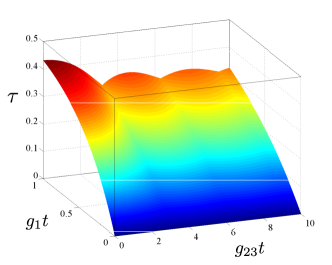
Figure 2: Nonclassicality depth $\tau$ as a function of the parameters $g_{1}t$ and $g_{23}t$.

The increasing values of $g_{1}t$ result in larger values of the nonclassicality depth $\tau$, as the number of photons simultaneously generated in modes 1 and 2 increases. We note that this pairing of photons in the process of parametric down-conversion is the only source of nonclassicality in the analyzed four-mode system. On the contrary, nonzero values of parameter $g_{23}t$ only lead to the oscillations of the nonclassicality depth $\tau$. This behavior occurs as the frequency up-conversion moves photons, and so also photon pairs, from modes 1 and 2 to modes 3 and 4 and vice versa (see the scheme in Fig. 1). This results in the nonclassical properties of modes 3 and 4, at the expenses of the nonclassical properties of modes 1 and 2.

The maximum value of the Lee nonclassicality depth $\tau=0.5$ is reached for $g_{23}t=0$ and ideally in the limit $g_{1}t\rightarrow\infty$, i.e. when only the strong parametric down-conversion occurs. This is in agreement with the analysis of nonclassical properties of twin beams reported in Ref. arkhipov15 . The value $\tau=0.5$ can also be asymptotically reached in the limit $g_{23}t\rightarrow\infty$, in which we have

$$\tau_{g_{23}t\to\infty}=\frac{1}{2}\left[\sqrt{(B_{1}-B_{2})^{2}+4|D_{12}|^{2}}-(B_{1}+B_{2})\right]$$ (13)

with $B_{3}\rightarrow B_{1}$, $B_{4}\rightarrow B_{2}$ and $D_{34}\rightarrow D_{12}$. It is worth noting that formula (13) applies also for $g_{23}t=0$.

Nonclassicality is also strongly resistant against damping in the system. This means that even a low number of photon pairs is sufficient to have a nonclassical state. We demonstrate this resistance by considering the damping constants $\gamma$ proportional to the nonlinear coupling constant $g_{1}$, which quantifies the speed of photon-pair generation. The graphs in Fig. 3 show that the generated states remain strongly nonclassical even though a considerable fraction of photon pairs is broken under these conditions. The comparison of graphs in Figs. 3(a) and (b) reveals that the damping is more detrimental in the down-converted modes 1 and 2 than in the up-converted modes 3 and 4.

At variance with nonclassicality, the determination and quantification of entanglement is more complex and it is technically accomplished by considering all possible bipartitions of the four-mode system (see the next Section). On the one side all bipartitions considered below are in principle sufficient to indicate entanglement, on the other side the application of the Van Loock and Furusawa inseparability criterion vanLoock03 to our system excludes the presence of genuine three- and four-mode entanglement. The analyzed Hamiltonian written in Eq. (1) together with the incident vacuum state also excludes the presence of nonclassical states in individual modes. In what follows, the bipartite entanglement is thus the only source of the global nonclassicality in the analyzed system. This situation considerably simplifies the possible experimental investigations as positive values of the Lee nonclassicality depth directly imply the presence of entanglement somewhere in the system.

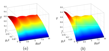
Figure 3: Nonclassicality depth $\tau$ as it depends on parameters $g_{1}t$ and $g_{23}t$ for (a) $\gamma_{1}t=\gamma_{2}t=g_{1}t$, $\gamma_{3}t=\gamma_{4}t=0$; (b) $\gamma_{1}t=\gamma_{2}t=0$, $\gamma_{3}t=\gamma_{4}t=g_{1}t$, assuming $n_{dj}=0$ for $j=1,\ldots,4$.

Four-mode entanglement

In quantifying the entanglement in our four-mode Gaussian system, we rely on the following facts applicable to an arbitrary $(m+n)$-mode Gaussian state. It has been proven that positivity of the partially transposed (PPT) statistical operator describing any $2\times 2$ or $2\times 3$ bipartition of the state is a necessary condition for the separability of the state Peres96 ; Horodecki97 . Moreover, it has been shown that the violation of PPT condition occurring in any $1\times(m+n-1)$ bipartitions or $m\times n$ bisymmetric bipartitions for $m>2$ and $n>3$ is a sufficient condition for the entanglement in the analyzed $(m+n)$-mode state Simon00 ; Serafini05 . For continuous variables systems, the PPT is simply accomplished when the symmetrically-ordered field operators are considered allowing to perform the PPT only by changing the signs of the momenta $\hat{p}$ Simon00 . Moreover, symplectic eiganvalues $\tilde{n}_{i}$ of the symmetrically-ordered covariance matrix $\sigma$ can be conveniently used to quantify entanglement in bipartite systems via the logarithmic negativity $E$ Vidal02 , defined in terms of eigenvalues $\tilde{n}_{i}<1/2$:

$$E=\max\left\{0,-\sum\limits_{i}{\mathrm{log}}(2\tilde{n}_{i})\right\},$$ (14)

where ${\rm max}$ gives the maximal value.

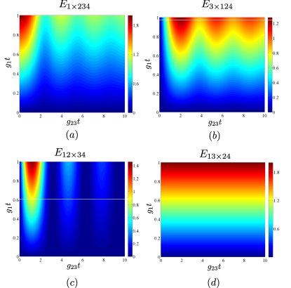
Figure 4: Logarithmic negativities $E_{1\times 234}$ (a), $E_{3\times 124}$ (b), $E_{12\times 34}$ (c), and $E_{13\times 24}$ (d) as functions of parameters $g_{1}t$ and $g_{23}t$ for different bipartitions indicated in the subscripts.

In the four-mode Gaussian state sketched in Fig. 1, we have two kinds of bipartitions. Either a single mode forms one subsystem and the remaining three modes belong to the other subsystem, or two modes are in one subsystem and the remaining two modes lie in the other subsystem. Due to the symmetry, only two members of each group are of interest for us. Namely, these are bipartitions $1\times 234$ and $3\times 124$ from the first group and bipartitions $12\times 34$ and $13\times 24$ from the second one. We note that, while the bipartition $12\times 34$ is bisymmetric in our interaction configuration (provided that $g_{2}t=g_{3}t$), the bipartition $13\times 24$ is not bisymmetric. Nevertheless, positive values of both the logarithmic negativities $E_{12\times 34}$ and $E_{13\times 24}$ reflect entanglement as both bipartitions involve two modes on both sides. Similarly, positive values of the logarithmic negativities $E_{1\times 234}$ and $E_{3\times 124}$ guarantee the presence of entanglement.

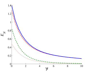
Figure 5: Logarithmic negativity $E$ as a function of the damping coefficient $\gamma t$ for different bipartitions: $1\times 234$ (dashed red line), $3\times 124$ (brown dotted line), $12\times 34$ (dashed-dotted green line), and $13\times 24$ (solid blue line). We set $g_{1}t=g_{2}t=g_{3}t=0.7$, $\gamma\equiv\gamma_{1}=\gamma_{2}=\gamma_{3}=\gamma_{4}$; $n_{dj}=0$ for $j=1,\ldots,4$.

We first pay attention to the entanglement expressed in the logarithmic negativities $E_{1\times 234}$ and $E_{3\times 124}$. As suggested by the graphs in Figs. 4(a) and (b), the oscillating behavior of negativity $E_{1\times 234}$ is complementary to that of negativity $E_{3\times 124}$. This means that the larger values of negativity $E_{1\times 234}$ are accompanied by the lower values of negativity $E_{3\times 124}$ and vice versa. Such a result is a consequence of the fact that the entanglement is due to the presence of photon pairs and a photon created in mode 1 can move to mode 3 and later return back to mode 1. This movement leads to the oscillations with frequency $g_{23}$, which are clearly visible in Figs. 4(a) and (b). This explanation also suggests that no entanglement is possible between modes 1 and 3. Indeed, if we also determine the negativity $E_{1\times 24}$ (or $E_{3\times 24}$), we will get the same values already obtained for the negativity $E_{1\times 234}$ ($E_{3\times 124}$).

The negativity $E_{12\times 34}$, characterizing the entanglement between the twin beam in modes 1 and 2 and the up-converted beams in modes 3 and 4, is plotted in Fig. 4(c). It reflects the gradual movement of photon pairs from modes 1 and 2, where they are created, to modes 3 and 4. Note that the maxima of negativity $E_{12\times 34}$ along the $g_{23}t$-axis occur inbetween the maxima of negativities $E_{1\times 234}$ and $E_{3\times 124}$. The origin of entanglement in photon pairing is confirmed in the graph of Fig. 4(d), showing that the negativity $E_{13\times 24}$ is independent of parameter $g_{23}t$ and that the negativity $E_{13\times 24}$ increases with the increasing parameter $g_{1}t$. In certain sense, the independence of negativity $E_{13\times 24}$ from parameter $g_{23}t$ represents the conservation law for nonclassical resources, as the negativities of the different two-mode reductions derived from this bipartition ($E_{1\times 2}$, $E_{1\times 4}$, $E_{3\times 2}$, and $E_{3\times 4}$) do depend on parameter $g_{23}t$.

The developed model also allows us to study the role of damping in the entanglement creation. The investigations based on equal damping constants $\gamma$ and noiseless reservoirs ($n_{d}=0$) just reveal the deterioration of entanglement in all the considered bipartitions with the increase of damping constants (see Fig. 5).

Two-mode entanglement and noise reduction factor

The results of the theoretical analysis suggest that, from the experimental point of view, the observation of entanglement between pairs of modes is substantial for the characterization of the emitted entangled states. Formally, the theory describes such observations through the reduced two-mode statistical operators. The analysis shows that the behavior of two-mode negativities $E_{1\times 2}$, $E_{3\times 4}$, and $E_{1\times 4}$ with respect to parameters $g_{1}t$ and $g_{23}t$ is qualitatively similar to that of four-mode negativities $E_{1\times 234}$, $E_{3\times 124}$, and $E_{12\times 34}$ plotted in Figs. 4(a), (b) and (c). This similarity originates in possible ‘trajectories’ of photon pairs born in modes 1 and 2 and responsible for the entanglement.

Additional insight into the generation of entanglement in the analyzed system is provided when the entanglement is related to the intensities of the interacting fields. As quantified in the graphs of Fig. 6, both mean photon numbers $B_{1}\equiv B_{2}$ and $B_{3}\equiv B_{4}$ are increasing functions of parameter $g_{1}t$ and oscillating functions of parameter $g_{23}t$. This oscillating behavior is particularly interesting, as it reflects the flow of photons from modes 1 and 2 to modes 3 and 4, respectively, and vice versa. As we will see below, this is in agreement with the ‘flow of the entanglement’ among the modes.

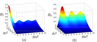
Figure 6: Mean photon numbers $B_{1}$ (a) and $B_{3}$ (b) plotted as functions of parameters $g_{1}t$ and $g_{23}t$.

The graph in Fig. 7(a) shows that the negativity $E_{1\times 2}$ is on the one side an increasing function of the mean photon number $B_{1}$, on the other side it only weakly depends on the mean photon number $B_{3}$. This confirms that pairing of photons in parametric down-conversion is the only resource for entanglement creation. On the contrary, as shown in Fig. 7(b), the negativity $E_{3\times 4}$ is an increasing function of the mean photon number $B_{3}$, whereas it weakly depends on the mean photon number $B_{1}$. This indicates that the entanglement in modes 34 comes from modes 12 through the transfer of photon pairs: The stronger the transfer is, the larger the value of negativity $E_{3\times 4}$ is. Moreover, optimal conditions for the observation of entanglement in modes 1 and 4 occur provided that there is the largest available number of photon pairs with one photon in mode 1 and its twin in mode 4. According to the graph in Fig. 7(c) this occurs when the mean photon numbers $B_{4}$ ($B_{4}\equiv B_{3}$) and $B_{1}$ are balanced, independently of their values.

In general, the experimental identification of two-mode entanglement is not easy, as it requires the simultaneous measurement of the entangled state in two complementary bases. Alternatively, entanglement can be inferred from the reconstructed two-mode phase-space quasi-distribution, which needs two simultaneous homodyne detectors Lvovsky2009 , each one endowed with a local oscillator. However, the detection of entanglement, at least in some cases, can be experimentally accomplished by the observation of sub-shot-noise intensity correlations. This is a consequence of the detailed numerical analysis,

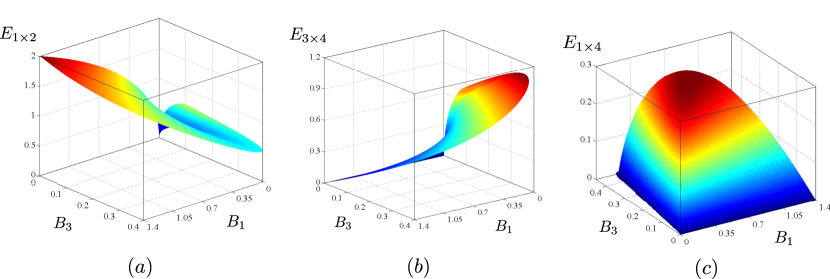
Figure 7: Logarithmic negativities $E_{1\times 2}$ (a), $E_{3\times 4}$ (b) and $E_{1\times 4}$ (c) as they depend on mean photon numbers $B_{1}$ and $B_{3}$.

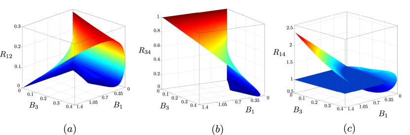
Figure 8: Noise reduction factors $R_{1\times 2}$ (a), $R_{3\times 4}$ (b) and $R_{1\times 4}$ (c) as they depend on mean photon numbers $B_{1}$ and $B_{3}$. In (c), the netted plane is defined as $R_{1\times 4}=1$.

which reveals that the majority of the reduced two-mode entangled states also exhibits sub-shot-noise intensity correlations. Nevertheless, it should be emphasized here that, in the analyzed system, there are also two-mode entangled states not exhibiting sub-shot-noise intensity correlations. On the contrary, we note that the reduced two-mode separable states do not naturally exhibit sub-shot-noise intensity correlations.

Sub-shot-noise intensity correlations are quantified by the noise reduction factor $R$ Degiovanni07 ; Degiovanni09 , that is routinely measured to recognize nonclassical intensity correlations of two optical fields. The noise reduction factor $R$ expressed in the moments of photon numbers $n_{j}$ and $n_{k}$ of modes $j$ and $k$, respectively, is defined by the formula:

$$R_{jk}=\frac{\langle\triangle(n_{j}-n_{k})^{2}\rangle}{\langle n_{j}\rangle+\langle n_{k}\rangle}.$$ (15)

Sub-shot-noise intensity correlations are described by the condition $R<1$. We note that there exists the whole hierarchy of inequalities involving higher-order moments of photon numbers (or intensities) Vogel2008 ; Miranowicz02 ; Miranowicz10 ; Allevi2012 that indicate nonclassicality and, in our system, also entanglement. We mention here the inequality derived by Lee Lee1990a as a practical example that is sometimes used in the experimental identification of nonclassicality. We note that this criterion is stronger than the noise reduction factor $R$ in revealing the nonclassicality Degiovanni07 .

The noise reduction factors $R_{1\times 2}$, $R_{3\times 4}$ and $R_{1\times 4}$ describing the reduced two-mode fields with their negativities plotted in Fig. 7 are drawn in Fig. 8 for comparison. We can see complementary behavior of the negativities $E$ and noise reduction factors $R$ in the graphs in Figs. 7 and 8. An increase of the negativity $E$ is accompanied by a decrease in the noise reduction factor $R$. A closer inspection of the curves in these graphs shows that the condition $R<1$ identifies very well entangled states when the noise reduction factor is measured in modes $1\times 2$ and $3\times 4$. Nevertheless, there are entangled states with $R_{1\times 4}>1$, as shown in the graph of Fig. 9, in which the values of parameters $g_{1}t$ and $g_{23}t$ appropriate for this situation occur in the areas I and III. On the other hand, the entangled states found in the area II in the graph of Fig. 9 have $R<1$. It is worth noting that the relative amount of entangled states not detected via $R<1$ increases with the increasing coupling constant $g_{1}t$ and so with the increasing overall number of photons in the system.

The observed relation between the entangled states and those exhibiting sub-shot-noise intensity correlations can even be explained theoretically, due to the specific form of the reduced two-mode Gaussian states analyzed in Ref. arkhipov15 . According to Ref. arkhipov15 entangled states in modes $i$ and $j$ are identified through the inequality $B_{i}B_{j}<|D_{ij}|^{2}$. On the other hand, the noise reduction factor $R_{ij}$ defined in Eq. (15) attains for our modes the form:

$$R_{ij}=1+\frac{B_{i}^{2}+B_{j}^{2}-2|D_{ij}|^{2}}{B_{i}+B_{j}}$$ (16)

that assigns the sub-shot-noise intensity correlations to the states obeying the inequality $B_{i}^{2}+B_{j}^{2}<2|D_{ij}|^{2}$. Thus, the inequality $B_{i}^{2}+B_{j}^{2}\geq 2B_{i}B_{j}$ implies that the states with sub-shot-noise intensity correlations form a subset in the set of all entangled states. Moreover, if $B_{i}=B_{j}$, both sets coincide as we have $B_{i}^{2}+B_{j}^{2}=2B_{i}B_{j}$. Thus, the noise reduction factors $R_{12}$ and $R_{34}$ are reliable in identifying entangled states in the symmetric case, in which $B_{1}=B_{2}$ and $B_{3}=B_{4}$.

We note that, according to the theory developed for the modes without an additional internal structure arkhipov15 , the logarithmic negativity $E_{ij}$ can be determined along the formula arkhipov15

$$E_{ij}={\rm max}\Big{\{}0, -\log\Big{(}1+B_{i}+B_{j}-$$ (17)

$$\sqrt{(B_{i}-B_{j})^{2}+4|D_{ij}|^{2}}\Big{)}\Big{\}},$$

where $|D_{ij}|^{2}=\langle\Delta n_{i}\Delta n_{j}\rangle$. According to Eq.  the logarithmic negativity $E_{ij}$ can, in principle, be inferred from the measured mean intensities in modes $i$ and $j$ and the cross-correlation function of intensity fluctuations in this idealized case.

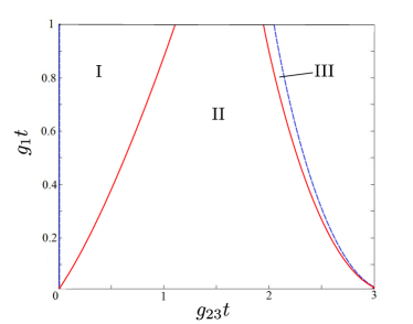
Figure 9: Solutions of the equations for logarithmic negativity $E_{1\times 4}=0$ (blue dashed line) and noise reduction factor $R_{1\times 4}=1$ (red solid line) in the plane spanned by parameters $g_{1}t$ and $g_{23}t$. The two-mode field is entangled [sub-shot-noise] ($E_{1\times 4}>0$ [$R_{1\times 4}<1$]) inbetween the blue dashed [red solid] lines, i.e. in the areas I, II, and III [II].

At the end, we make a note about the entanglement in the general four-mode system with different up-conversion coupling constants ($g_{2}\neq g_{3}$). This is relevant when non-ideal phase-matching conditions of the three nonlinear interactions are met in the experiment (see below). According to our investigations, the largest values of negativities $E_{1\times 2}$ and $E_{3\times 4}$ are found in the symmetric four-mode system ($g_{2}=g_{3}$) considered above. On the contrary, the largest values of negativities $E_{1\times 4}$ and $E_{2\times 3}$ are obtained for unbalanced $g_{2}$ and $g_{3}$ interactions.

Similarly to the symmetric case, separable states, entangled states without sub-shot-noise intensity correlations and entangled states exhibiting sub-shot-noise intensity correlations are found in the whole three-dimensional parametric space spanned by variables $g_{j}t$ for $j=1,2,3$. As an example, the distribution of different kinds of reduced two-mode states found in the up-converted modes 3 and 4 in this space is plotted in Fig. 10. The graphs in Fig. 10 indicate that, in accord with the symmetric case, the larger the value of constant $g_{1}t$, the larger the relative amount of entangled states that cannot be identified through sub-shot-noise intensity correlations.

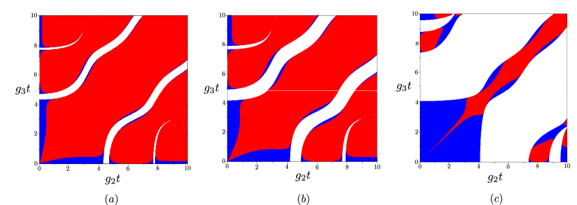
Figure 10: Planes given by $g_{1}t=0.5$ (a), $g_{1}t=1$ (b) and $g_{1}t=5$ (c) in the ’phase diagram’ identifying classical states (white areas), entangled states without sub-shot-noise intensity correlations (blue) and entangled states with sub-shot-noise intensity correlations (red) in the space spanned by the coupling constants $g_{j}t$, $j=1,2,3$.

Experimental implementation

A possible experimental implementation of the four mode interaction described above can be achieved by using a BaB₂O₄ crystal as the nonlinear medium, a ps-pulsed laser (a mode-locked Nd:YLF laser regeneratively amplified at 500 Hz, High-Q Laser Production) to get the pump fields and hybrid photodetectors (mod. R10467U-40, Hamamatsu Photonics) as the photon-number-resolving detectors. A typical experimental setup can be built in analogy with other previous experiments Allevi2012 . The phase-matching conditions can be chosen so as to have $\omega_{1}=\omega_{2}$ and a common pump field for both up-conversion processes so that $\omega_{3}=\omega_{4}$. In this specific symmetric case we have $g_{2}=g_{3}\equiv g_{23}$.

We can estimate the range of coupling constants achievable in this setup based on the above-mentioned laser source. Let us consider the following parameters: wavelength of the pump for down-conversion $\lambda_{p1}=349$ nm, $\lambda_{1}=\lambda_{2}=698$ nm, wavelength of the pump for up-conversion $\lambda_{p2}=1047$ nm, $\lambda_{3}=\lambda_{4}=418.8$ nm, length of the BaB₂O₄ crystal $L=4$ mm, diameters of the pumps 0.5 mm, pulse duration 4.5 ps. The coupling constants $g_{1}$ and $g_{23}$ are linearly proportional to the corresponding pump field amplitudes so that $g_{1}t=\kappa_{1}A_{p1}L$ and $g_{23}t=\kappa_{23}A_{p2}L$, where $\kappa_{j}$ ($j=1,23$) are the nonlinear coupling coefficients and $A_{j}$ ($j=p1,p2$) are the pump amplitudes. For the considered parameters we can estimate $\kappa_{j}\approx 10^{-13}s^{1/2}$. The useful range of energies per pulse is up to 66 $\mu$J in the UV and up to 240 $\mu$J in the IR, corresponding to maximum values $g_{1}t\approx 5.9$ and $g_{2}t\approx 7$. The theoretical results discussed above predict an interesting behavior for this range of parameters, including the transfer of entanglement into the up-converted modes.

Conclusions

Four-mode Gaussian states generated via parametric down-conversion and frequency up-conversion have been analyzed in terms of nonclassicality, entanglement and entanglement transfer among the modes. While nonclassicality of the state has been described by the easily-computable Lee nonclassicality depth, logarithmic negativity for different bipartitions has been applied to monitor the occurrence of entanglement among different modes. It has been shown that whenever the analyzed system is nonclassical, it is also entangled. Moreover, the entanglement is present only in the form of bipartite entanglement. The analysis of the noise reduction factor identifying sub-shot-noise intensity correlations, in parallel with the logarithmic negativity quantifying two-mode entanglement, has shown that the noise reduction factor is a powerful indicator of the entanglement in the analyzed system. This is substantial for the experimental demonstration of the transfer of entanglement from the down-converted modes to the up-converted ones.

Acknowledgments This work was supported by the projects No. 15-08971S of the GA ČR and No. LO1305 of the MŠMT ČR. I.A. thanks project IGA_2016_002 UP Olomouc. The authors also acknowledge support from the bilateral Czech-Italian project CNR-16-05 between CAS and CNR.

Author contributions statement I.A., J.P., O.H., A.A. and M.B. developed the theory. I.A. prepared the figures. I.A., J.P., O.H., A.A. and M.B. wrote the manuscript. All authors reviewed the manuscript.

Appendix A The evolution matrix ${\bf M}$

The evolution matrix ${\bf M}$ describing the operator solution of the Heisenberg equations written in Eq. (2) is derived in the form:

$${\bf M}=\Large\left(\begin{array}[]{cccc}{\frac{x{c_{1}}-y{c_{2}}}{x-y}}&{\frac{ixy\left(\sqrt{{y_{1}}}{s_{2}}-\sqrt{{x_{1}}}{s_{1}}\right)}{\left(x{y_{1}}-{x_{1}}\,y\right){g_{1}}}}&{\frac{i\left(y\sqrt{{y_{1}}}{x_{1}}\,{s_{2}}-x\sqrt{{x_{1}}}{y_{1}}\,{s_{1}}\right)}{{g_{2}}\,\left(x{y_{1}}-{x_{1}}\,y\right)}}&{\frac{xy\left({c_{2}}-{c_{1}}\right)}{{g_{1}}\,{g_{3}}\,\left(x-y\right)}}\\ \vskip 6.0pt plus 2.0pt minus 2.0pt\cr{\frac{i{g_{1}}\,\left(\sqrt{{y_{1}}}{s_{2}}-\sqrt{{x_{1}}}{s_{1}}\right)}{x-y}}&{\frac{x{y_{1}}\,{c_{2}}-{x_{1}}\,y{c_{1}}}{x{y_{1}}-{x_{1}}\,y}}&{\frac{{g_{1}}\,{y_{1}}\,{x_{1}}\,\left({c_{2}}-{c_{1}}\right)}{{g_{2}}\,\left(x{y_{1}}-{x_{1}}\,y\right)}}&{\frac{i\left(\sqrt{{y_{1}}}x{s_{2}}-\sqrt{{x_{1}}}y{s_{1}}\right)}{\left(x-y\right){g_{3}}}}\\ \vskip 6.0pt plus 2.0pt minus 2.0pt\cr{\frac{i{g_{2}}\,\left(\sqrt{{x_{1}}}y{s_{2}}-\sqrt{{y_{1}}}x{s_{1}}\right)}{\sqrt{{x_{1}}}\left(x-y\right)\sqrt{{y_{1}}}}}&-{\frac{{g_{2}}\,xy\left({\it c_{2}}-{c_{1}}\right)}{\left(x{y_{1}}-{x_{1}}\,y\right){g_{1}}}}&{\frac{x{y_{1}}\,{c_{1}}-{x_{1}}\,y{c_{2}}}{x{y_{1}}-{x_{1}}\,y}}&{\frac{-i{g_{2}}\,xy\left(\sqrt{{x_{1}}}{s_{2}}-\sqrt{{y_{1}}}{s_{1}}\right)}{{g_{1}}\,{g_{3}}\,\left(x-y\right)\sqrt{{x_{1}}}\sqrt{{y_{1}}}}}\\ \vskip 6.0pt plus 2.0pt minus 2.0pt\cr{\frac{{g_{1}}\,{g_{3}}\,\left(-{c_{2}}+{c_{1}}\right)}{x-y}}&{\frac{i{g_{3}}\,\left(\sqrt{{y_{1}}}x{s_{2}}-\sqrt{{x_{1}}}y{s_{1}}\right)}{x{y_{1}}-{x_{1}}\,y}}&{\frac{i{g_{1}}\,{g_{3}}\,\left({x_{1}}\,\sqrt{{y_{1}}}{s_{2}}-{y_{1}}\,\sqrt{{x_{1}}}{s_{1}}\right)}{{g_{2}}\,\left(x{y_{1}}-{x_{1}}\,y\right)}}&{\frac{x{c_{2}}-y{c_{1}}}{x-y}}\end{array}\right)$$ (22)

where $x=(a+b)/2$, $x_{1}=(a_{1}+b)/2$, $y=(a-b)/2$, $y_{1}=(a_{1}-b)/2$, $a=-g_{1}^{2}+g_{2}^{2}-g_{3}^{2}$, $a_{1}=-g_{1}^{2}+g_{2}^{2}+g_{3}^{2}$, $b=\sqrt{{{g_{1}}}^{4}-2\,{{g_{1}}}^{2}{{g_{2}}}^{2}-2\,{{g_{1}}}^{2}{{g_{3}}}^{2}+{{g_{2}}}^{4}-2\,{{g_{2}}}^{2}{{g_{3}}}^{2}+{{g_{3}}}^{4}}$, $c_{1}=\cos(\sqrt{x_{1}}t)$, $c_{2}=\cos(\sqrt{y_{1}}t)$, $s_{1}=\sin(\sqrt{x_{1}}t)$, and $s_{2}=\sin(\sqrt{y_{1}}t)$.

References

- (1) Aspect, A., Dalibard, J. & Roger, G. Experimental test of bell’s inequalities using time- varying analyzers. Phys. Rev. Lett. 49, 1804–1807 (1982).
- (2) Weihs, G., Jennewein, T., Simon, C., Weinfurter, H. & Zeilinger, A. Violation of Bell’s inequality under strict Einstein locality conditions. Phys. Rev. Lett. 81, 5039 (1998).
- (3) Brunner, N., Cavalcanti, D., Pironio, S., Scarani, V. & Wehner, S. Bell nonlocality. Rev. Mod. Phys. 86, 419–478 (2014).
- (4) Bouwmeester, D. et al. Experimental quantum teleportation. Nature 390, 575–579 (1997).
- (5) Genovese, M. Research on hidden variable theories: A review of recent progresses. Phys. Rep. 413, 319—396 (2005).
- (6) Nielsen, M. A. & Chuang, I. L. Quantum Computation and Quantum Information (Cambridge University Press, Cambridge, UK, 2000).
- (7) Aoki, T. et al. Experimental creation of a fully inseparable tripartite continuous-variable state. Phys. Rev. Lett. 91, 080404 (2003).
- (8) van Loock, P. & Braunstein, S. L. Telecloning of continuous quantum variables. Phys. Rev. Lett. 87, 247901 (2001).
- (9) Yonezawa, H., Aoki, T. & Furusawa, A. Demonstration of a quantum teleportation network for continuous variables. Nature 431, 430 (2004).
- (10) Bouwmeester, D., Ekert, A. & Zeilinger, A. The Physics of Quantum Information (Springer, Berlin, 2000).
- (11) Dodonov, V. V. Nonclassical states in quantum optics: A squeezed review of the first 75 years. J. Opt. B: Quantum Semiclass. Opt. 4, R1—R33 (2002).
- (12) Allevi, A., Bondani, M., Paris, M. G. A. & Andreoni, A. Demonstration of a bright and compact source of tripartite nonclassical light. Phys. Rev. A 78, 063801 (2008).
- (13) Coelho, A. S. et al. Three-color entanglement. Science 326, 823 (2009).
- (14) Pysher, M., Miwa, Y., Shahrokhshahi, R., Bloomer, R. & Pfister, O. Parallel generation of quadripartite cluster entanglement in the optical frequency comb. Phys. Rev. Lett. 107, 030505 (2011).
- (15) Boyd, R. W. Nonlinear Optics, 2nd edition (Academic Press, New York, 2003).
- (16) Mandel, L. & Wolf, E. Optical Coherence and Quantum Optics (Cambridge Univ. Press, Cambridge, 1995).
- (17) Peřina, J. Quantum Statistics of Linear and Nonlinear Optical Phenomena (Kluwer, Dordrecht, 1991).
- (18) Langrock, C. et al. Highly efficient single-photon detection at communication wavelengths by use of upconversion in reverse-proton-exchanged periodically poled LiNBO3 waveguides. Opt. Lett. 30, 1725–1727 (2005).
- (19) Ramelow, S., Fedrizzi, A., Poppe, A., Langford, N. K. & Zeilinger, A. Polarization-entanglement-conserving frequency conversion of photons. Phys. Rev. A 85, 013845 (2012).
- (20) Lee, C. T. Measure of the nonclassicality of nonclassical states. Phys. Rev. A 44, R2775 (1991).
- (21) Arkhipov, I. I., Peřina Jr., J., Svozilík, J. & Miranowicz, A. Nonclassicality invariant of general two-mode Gaussian states. Sci. Rep. 6, 26523 (2016).
- (22) van Loock, P. & Furusawa, A. Detecting genuine multipartite continuous-variable entanglement. Phys. Rev. A 67, 052315 (2003).
- (23) Peres, A. Separability criterion for density matrices. Phys. Rev. Lett 77, 1413 (1996).
- (24) Horodecki, P. Separability criterion and inseparable mixed states with positive partial transposition. Phys. Lett. A 232, 333 (1997).
- (25) Hill, S. & Wootters, W. K. Computable entanglement. Phys. Rev. Lett. 78, 5022 (1997).
- (26) Vidal, G. & Werner, R. F. Computable measure of entanglement. Phys. Rev. A 65, 032314 (2002).
- (27) Vogel, W. Nonclassical correlation properties of radiation fields. Phys. Rev. Lett. 100, 013605 (2008).
- (28) Waks, E., Diamanti, E., Sanders, B. C., Bartlett, S. D. & Yamamoto, Y. Direct observation of nonclassical photon statistics in parametric down-conversion. Phys. Rev. Lett. 92, 113602 (2004).
- (29) Haderka, O., Peřina Jr., J., Hamar, M. & Peřina, J. Direct measurement and reconstruction of nonclassical features of twin beams generated in spontaneous parametric down-conversion. Phys. Rev. A 71, 033815 (2005).
- (30) Avenhaus, M. et al. Photon number statistics of multimode parametric down-conversion. Phys. Rev. Lett. 101, 053601 (2008).
- (31) Peřina Jr., J., Hamar, M., Michálek, V. & Haderka, O. Photon-number distributions of twin beams generated in spontaneous parametric down-conversion and measured by an intensified CCD camera. Phys. Rev. A 85, 023816 (2012).
- (32) Sperling, J., Vogel, W. & Agarwal, G. S. True photocounting statistics of multiple on-off detectors. Phys. Rev. A 85, 023820 (2012).
- (33) Allevi, A., Olivares, S. & Bondani, M. Measuring high-order photon-number correlations in experiments with multimode pulsed quantum states. Phys. Rev. A 85, 063835 (2012).
- (34) Peřina Jr., J. & Peřina, J. Quantum statistics of nonlinear optical couplers. In Wolf, E. (ed.) Progress in Optics, Vol. 41, 361—419 (Elsevier, Amsterdam, 2000).
- (35) Arkhipov, I. I., J. Peřina Jr., J. Peřina & Miranowicz, A. Comparative study of nonclassicality, entanglement, and dimensionality of multimode noisy twin beams. Phys. Rev. A 91, 033837 (2015).
- (36) Simon, R. Peres-Horodecki separability criterion for continuous variable systems. Phys. Rev. Lett 84, 2726 (2000).
- (37) Serafini, A., Adesso, G. & Illuminati, F. Unitarily localizable entanglement of gaussian states. Phys. Rev. A. 71, 032349 (2005).
- (38) A. I. Lvovsky and M. G. Raymer. Continuous-variable optical quantum state tomography. Rev. Mod. Phys. 81, 299 (2009).
- (39) Degiovanni, I. P., Bondani, M., Puddu, E., Andreoni, A. & Paris, M. G. A. Intensity correlations, entanglement properties, and ghost imaging in multimode thermal-seeded parametric down-conversion: Theory. Phys. Rev. A 76, 062609 (2007).
- (40) Degiovanni, I. P. et al. Monitoring the quantum-classical transition in thermally seeded parametric down-conversion by intensity measurements. Phys. Rev. A 79, 063836 (2009).
- (41) Richter, T. & Vogel, W. Nonclassicality of quantum states: A hierarchy of observable conditions. Phys. Rev. Lett. 89, 283601 (2002).
- (42) Miranowicz, A., Bartkowiak, M., Wang, X., Liu, Y. X. & Nori, F. Testing nonclassicality in multimode fields: A unified derivation of classical inequalities. Phys. Rev. A 82, 013824 (2010).
- (43) Lee, C. T. Higher-order criteria for nonclassical effects in photon statistics. Phys. Rev. A 41, 1721 (1990).