Semiparametric clustered overdispersed multinomial goodness-of-fit of log-linear models

Abstract

Traditionally, the Dirichlet-multinomial distribution has been recognized as a key model for contingency tables generated by cluster sampling schemes. There are, however, other possible distributions appropriate for these contingency tables. This paper introduces new test-statistics capable to test log-linear modeling hypotheses with no distributional specification, when the individuals of the clusters are possibly homogeneously correlated. The estimator for the intracluster correlation coefficient proposed in Alonso-Revenga et al. (2016), valid for different cluster sizes, plays a crucial role in the construction of the goodness-of-fit test-statistic.

Keywords: Clustered Multinomial Data; Consistent Intracluster Correlation Estimator; Log-linear model; Overdispersion; Quasi Minimum Divergence Estimator.

1 Introduction

In studies of frequency data, often the observations are organized in clusters. For clustered frequency data the classical statistical procedures are not longer valid. For example, in a study of hospitalized pairs of siblings, it is desired to study wether gender has any influence in schizophrenic diagnosis. Since the two outcomes of every pair of siblings (a cluster) are correlated for all the $N$ pairs of siblings, the assumption of independence of all the $2N$ observations is violated and the classical independence test of two categorical variables, gender and schizophrenic diagnosis, is in principle useless. The same problem of invalidity of the classical chi-square and likelihood ratio tests are presented with any statistical model used for clustered frequencies.

Frequency data cross-classified according to $K$ variables, $(X_{1},...,X_{K})$, having $X_{k}$ categories $1,2,...,I_{k}$, $k=1,...,K$, are the so-called $K$-way contingency tables with $M=I_{1}\times I_{2}\times\cdots\times I_{K}$ cells. In order to clarify the concepts and notation we will focus our interest only on $K=2$ variables, $(X_{1},X_{2})$, with $I$ and $J$ categories respectively, i.e. it has $M=I\times J$ cells denoted by pairs lexicographically ordered as

$$\Omega=\{(1,1),(1,2),...,(1,J),....,(I,1),(I,2),...,(I,J)\},$$

but it is possible to extend easily the same idea to $K$ variables. The bidimensional random variable associated with the $\ell$-th cluster of size $n_{\ell}$, $\ell=1,...,N$, being $N$ the number of clusters, is denoted as

$$(X_{1,h}^{(\ell)},X_{2,h}^{(\ell)}),\quad\ell=1,...,N,\;h=1,...,n_{\ell}.$$

Let

$$\mathrm{I}_{S}(X_{1},X_{2})=\left\{\begin{array}[c]{ll}1,&\text{if }(X_{1},X_{2})\in S\\ 0,&\text{if }(X_{1},X_{2})\notin S\end{array}\right.$$

denote an indicator function of $S\subset\Omega$. Taking into account the total count associated with cell $(i,j)$ is

$$Y_{ij}^{(\ell)}=\sum_{h=1}^{n_{\ell}}\mathrm{I}_{\{(i,j)\}}(X_{1,h}^{(\ell)},X_{2,h}^{(\ell)}),\quad\ell=1,...,N,$$ (1.1)

the $\ell$-th two-way frequency table in vector notation is given

$$\boldsymbol{Y}^{(\ell)}=(Y_{11}^{(\ell)},...,Y_{1J}^{(\ell)},...,Y_{I1}^{(\ell)},...,Y_{IJ}^{(\ell)})^{T},\quad\ell=1,...,N,$$

where “^T” denotes the transpose of a vector or matrix. In what follows, it is assumed an homogeneous probability for each individual felt in cell $(i,j)$ of the $\ell$-th cluster

$$p_{ij}(\boldsymbol{\theta})=\Pr(X_{1,h}^{(\ell)}=i,X_{2,h}^{(\ell)}=j),\quad\ell=1,...,N,\;h=1,...,n_{\ell},$$

whose expression depends on an unknown $M_{0}$-dimensional parameter vector

$$\boldsymbol{\theta}=(\theta_{1},...,\theta_{M_{0}})^{T}\in\mathbb{R}^{M_{0}},$$

in terms of a log-linear model

$$\boldsymbol{p}(\boldsymbol{\theta})=\frac{\exp\{\boldsymbol{W\theta}\}}{\boldsymbol{1}_{M}^{T}\exp\{\boldsymbol{W\theta}\}},$$ (1.2)

where $M_{0}<M-1$,

$$\boldsymbol{p}(\boldsymbol{\theta})=(p_{11}(\boldsymbol{\theta}),...,p_{1J}(\boldsymbol{\theta}),...,p_{I1}(\boldsymbol{\theta}),...,p_{IJ}(\boldsymbol{\theta}))^{T}$$ (1.3)

and the design matrix, $\boldsymbol{W}$, is a full rank matrix, with column vectors linearly independent with respect to the $M$-dimensional vector of $1$’s, $\boldsymbol{1}_{M}=(1,...,1)^{T}$.

Under common correlation model for any pair of individuals $h$ and $s$ ($h,s=1,...,n_{\ell},\;h\neq s$) of any cluster $\ell=1,...,N$, the intracluster correlation coefficient is defined as

$$\rho_{ij}^{2} =\mathrm{Cor}[\mathrm{I}_{\{(i,j)\}}(X_{1,h}^{(\ell)},X_{2,h}^{(\ell)}),\mathrm{I}_{\{(i,j)\}}(X_{1,s}^{(\ell)},X_{2,s}^{(\ell)})]$$

$$=\frac{\mathrm{E}[\mathrm{I}_{\{(i,j)\}}(X_{1,h}^{(\ell)},X_{2,h}^{(\ell)})\mathrm{I}_{\{(i,j)\}}(X_{1,s}^{(\ell)},X_{2,s}^{(\ell)})]-\mathrm{E}[\mathrm{I}_{\{(i,j)\}}(X_{1,h}^{(\ell)},X_{2,h}^{(\ell)})]E[\mathrm{I}_{\{(i,j)\}}(X_{1,s}^{(\ell)},X_{2,s}^{(\ell)})]}{\sqrt{\mathrm{Var}(\mathrm{I}_{\{(i,j)\}}(X_{1,h}^{(\ell)},X_{2,h}^{(\ell)}))\mathrm{Var}(\mathrm{I}_{\{(i,j)\}}(X_{1,s}^{(\ell)},X_{2,s}^{(\ell)}))}}$$

$$=\frac{\Pr(X_{1,h}^{(\ell)}=X_{1,s}^{(\ell)}=i,X_{2,h}^{(\ell)}=X_{2,s}^{(\ell)}=j)-p_{ij}^{2}(\boldsymbol{\theta})}{p_{ij}(\boldsymbol{\theta})\left(1-p_{ij}(\boldsymbol{\theta})\right)},\quad\ell=1,...,N,\;h,s=1,...,n_{\ell},\;h\neq s$$

(see Eldridge et al. (2009), for more details). In correlated clustered overdispersed multinomial frequency data, in case of having homogeneous intracluster correlation cell by cell, $\rho^{2}=\rho_{ij}^{2}$, $i=1,...I$, $j=1,...,J$ and for this case, taking into account (1.1) and

$$\mathrm{E}[\mathrm{I}_{\{(i,j)\}}(X_{1,h}^{(\ell)},X_{2,h}^{(\ell)})] =p_{ij}(\boldsymbol{\theta}),$$

$$\mathrm{Cov}[\mathrm{I}_{\{(i,j)\}}(X_{1,h}^{(\ell)},X_{2,h}^{(\ell)}),I_{\{(i,j)\}}(X_{1,s}^{(\ell)},X_{2,s}^{(\ell)})] =\left\{\begin{array}[c]{ll}\rho^{2}p_{ij}(\boldsymbol{\theta})\left(1-p_{ij}(\boldsymbol{\theta})\right),&h\neq s\\ p_{ij}(\boldsymbol{\theta})\left(1-p_{ij}(\boldsymbol{\theta})\right),&h=s\end{array}\right.,$$

it is proven that

$$\mathrm{E}[\boldsymbol{Y}^{(\ell)}]=n_{\ell}\boldsymbol{p}(\boldsymbol{\theta})\quad\text{and}\quad\mathrm{Var}[\boldsymbol{Y}^{(\ell)}]=\vartheta_{n_{\ell}}n_{\ell}\boldsymbol{\Sigma}_{\boldsymbol{p}(\boldsymbol{\theta})},$$ (1.4)

where

$$\vartheta_{n_{\ell}}=1+(n_{\ell}-1)\rho^{2},$$ (1.5)

is referred to as “design effect” associated with the $\ell$-th cluster,

$$\boldsymbol{\Sigma}_{\boldsymbol{p}(\boldsymbol{\theta})}=\boldsymbol{D}_{\boldsymbol{p}(\boldsymbol{\theta})}-\boldsymbol{p}(\boldsymbol{\theta})\boldsymbol{p}^{T}(\boldsymbol{\theta}),$$ (1.6)

and $\boldsymbol{D}_{\boldsymbol{p}(\boldsymbol{\theta})}$ is the diagonal matrix of $\boldsymbol{p}(\boldsymbol{\theta})$. Since $\mathrm{Var}[Y_{ij}^{(\ell)}]>0$, it holds $\vartheta_{n_{\ell}}=1+(n_{\ell}-1)\rho^{2}>0$ for $\ell=1,...,N$ and thus $\rho^{2}>-1/(\max\{n_{\ell}\}_{\ell=1}^{N}-1)$, but in practice it is assumed that $\rho^{2}\geq 0$. This is just the reason why these models are termed “overdispersed models”. In particular, for $\rho^{2}=0$ all the frequency tables are multinomial.

Correlated clustered multinomial frequency data have been dealt in the statistical literature since many years ago through two different approaches. Following Choi and McHugh (1989), the design-based approach provides inferences with respect to the sampling distribution of estimates over repetitions of the same design. The works of Fellegi (1980), Holt et al. (1980), Rao and Scott (1981,1984), Bedrick (1983), Landis et al (1984), Koch et al. (1975), Fay (1985), as well as references therein are good examples of this approach. On the other hand, Altham (1976), Cohen (1976), Brier (1980), Fienberg (1979), Menéndez et al. (1995, 1996) postulate a probability distribution to model the sample data. Dirichlet-multinomial is, historically, the first suitable distribution to modelize homogeneously correlated clustered overdispersed multinomial frequency with a fixed cluster size (see Mosimann, 1962). Later, Cohen (1976) and Altham (1976) proposed the $n$-inflated distribution and more recently, Morel and Nagaraj (1993) proposed the random-clumped distribution. The zero-inflated binomial distribution falls also inside this family of homogeneously correlated clustered overdispersed multinomial frequency data. Details about these distributions can be found in Alonso-Revenga et al. (2016). In the current paper and in Alonso-Revenga et al. (2016) a third approach is presented, different from the previous ones, based on the sole knowledge of the vector mean and the variance-covariance matrix of the distribution, given in (1.4), associated with the generator of the sample data. For log-linear modeling no distribution assumption is required if the quasi minimum $\phi$-divergence estimators are used. In the following we shall assume that the data are generated by a population verifying (1.4). One of the strengths of this methodology, is that the proposed consistent estimator for $\rho^{2}$ is semi-parametric and it exhibits by far a better behavior with regard to the mean square error (MSE) in comparison with the existing estimation method, which is fully non-parametric. This kind of estimators are specially appealing for improving the behavior of the existing goodness-of-fit tests for log-linear models, with regard to the exact sizes and powers. The second strength of this methodology, is the flexibility in being applicable for different cluster sizes.

For the semiparametric clustered overdispersed multinomial goodness-of-fit of log-linear models, the interest lays on testing wether it holds a particular log-linear model

$$H_{0}:\;\boldsymbol{p}(\boldsymbol{\theta})=\frac{\exp\{\boldsymbol{W\theta}\}}{\boldsymbol{1}_{M}^{T}\exp\{\boldsymbol{W\theta}\}}\quad\text{vs.}\quad H_{1}:\;\boldsymbol{p}(\boldsymbol{\theta})\neq\frac{\exp\{\boldsymbol{W\theta}\}}{\boldsymbol{1}_{M}^{T}\exp\{\boldsymbol{W\theta}\}}.$$ (1.7)

2 Asymptotic Goodness-Of-Fit (GOF) test-statistics for equal cluster sizes

For the frequency tables and the probability vectors, a single index notation is preferred, since it covers any value, $K$, for the dimension of the contingency table. This means that the probability vector

$$\boldsymbol{p}(\boldsymbol{\theta})=(p_{1}(\boldsymbol{\theta}),...,p_{M}(\boldsymbol{\theta}))^{T},$$

and the $\ell$-th frequency table

$$\boldsymbol{Y}^{(\ell)}=(Y_{1}^{(\ell)},...,Y_{M}^{(\ell)})^{T},\quad\ell=1,...,N,$$ (2.1)

are valid to represent double index elements ordered as (1.3) when $K=2$ ($M=IJ$), as well as to generalize for any value of $K$ when the $K$-tuples are lexicographically ordered ($M=\prod_{k=1}^{K}I_{k}$). The $M$-dimensional vector obtained from collapsing the whole data, $\boldsymbol{Y}^{(\ell)}$, $\ell=1,...,N$, is denoted by

$$\boldsymbol{Y}=\sum_{\ell=1}^{N}\boldsymbol{Y}^{(\ell)}$$

and $MN$-dimensional vector which gathers the whole data, $\boldsymbol{Y}^{(\ell)}$, $\ell=1,...,N$, by

$$\widetilde{\boldsymbol{Y}}=(\boldsymbol{Y}^{(1)T},...,\boldsymbol{Y}^{(N)T})^{T}.$$

In this section, a family of GOF test-statistics for testing (1.7) with equal cluster sizes is introduced. In the following section the case of unequal cluster sizes is treated. Some preliminary results related to the estimators of the probability vector, derived in Alonso-Revenga et al. (2016), are first introduced. The non-parametric estimator of $\boldsymbol{p}(\boldsymbol{\theta})$, based on $N$ clusters of sizes $n_{\ell}=n$, $\ell=1,...,N$, is the $M$-dimensional vector of relative frequencies obtained collapsing the $N$ frequency tables $\boldsymbol{Y}^{(\ell)}$, $\ell=1,...,N$,

$$\widehat{\boldsymbol{p}}=\frac{1}{nN}\boldsymbol{Y}=\frac{1}{nN}\sum_{\ell=1}^{N}\boldsymbol{Y}^{(\ell)}=\frac{1}{N}\sum_{\ell=1}^{N}\widehat{\boldsymbol{p}}^{(\ell)},$$

where $\widehat{\boldsymbol{p}}^{(\ell)}=\tfrac{1}{n}\boldsymbol{Y}^{(\ell)}$ represents the non-parametric estimator of $\boldsymbol{p}(\boldsymbol{\theta})$ based exclusively on the $\ell$-th cluster.

Based on the collapsed table, $\boldsymbol{Y}$, the quasi minimum $\phi$-divergence estimator (QM$\phi$E) of $\boldsymbol{\theta}$ in (1.2) is defined as

$$\widehat{\boldsymbol{\theta}}_{\phi}=\widehat{\boldsymbol{\theta}}_{\phi}\left(\boldsymbol{Y}\right)=\arg\min_{\theta\in\Theta}d_{\phi}(\widehat{\boldsymbol{p}},\boldsymbol{p}\left(\boldsymbol{\theta}\right)),$$

where $\phi\left(x\right)$ is a convex function, $x>0$, such that at $x=1$, $\phi\left(1\right)=0$, $\phi^{\prime}\left(1\right)=0$, $\phi^{\prime\prime}\left(1\right)>0$, at $x=0$, $0\phi\left(0/0\right)=0$, $0\phi\left(p/0\right)=\underset{u\rightarrow\infty}{\lim}p\phi\left(u\right)/u$, and

$$\mathrm{d}_{\phi}\left(\widehat{\boldsymbol{p}},\boldsymbol{p}\left(\boldsymbol{\theta}\right)\right)=\sum\limits_{r=1}^{M}p_{r}\left(\boldsymbol{\theta}\right)\phi\!\left(\frac{\widehat{p}_{r}}{p_{r}\left(\boldsymbol{\theta}\right)}\right)$$ (2.2)

is the $\phi$-divergence between the probability vectors $\widehat{\boldsymbol{p}}$ and $\boldsymbol{p}\left(\boldsymbol{\theta}\right)$. For more details about $\phi$-divergence measures see Cressie and Pardo (2002) and Pardo (2006).

The quasi-maximum likelihood estimator (QMLE) of $\boldsymbol{\theta}$, denoted by $\widehat{\boldsymbol{\theta}}$, is a particular case of the QM$\phi$E by replacing the $\phi$-divergence by the Kullback divergence between the probability vectors $\widehat{\boldsymbol{p}}$ and $\boldsymbol{p}\left(\boldsymbol{\theta}\right)$, i.e.,

$$\widehat{\boldsymbol{\theta}}=\widehat{\boldsymbol{\theta}}\left(\boldsymbol{Y}\right)=\arg\min_{\theta\in\Theta}\mathrm{d}_{Kullback}(\widehat{\boldsymbol{p}},\boldsymbol{p}\left(\boldsymbol{\theta}\right)),$$

$$\mathrm{d}_{Kullback}(\widehat{\boldsymbol{p}},\boldsymbol{p}\left(\boldsymbol{\theta}\right))=\sum\limits_{r=1}^{M}\widehat{p}_{r}\log\frac{\widehat{p}_{r}}{p_{r}\left(\boldsymbol{\theta}\right)},$$

or equivalently $\widehat{\boldsymbol{\theta}}=\widehat{\boldsymbol{\theta}}\left(\boldsymbol{Y}\right)=\arg\min_{\theta\in\Theta}d_{\phi}(\widehat{\boldsymbol{p}},\boldsymbol{p}\left(\boldsymbol{\theta}\right))$, with $\phi(x)=x\log x-x+1$. Since the QM$\phi$Es are invariant estimators,

$$\boldsymbol{p}(\widehat{\boldsymbol{\theta}}_{\phi})=\frac{\exp\{\boldsymbol{W}\widehat{\boldsymbol{\theta}}_{\phi}\}}{\boldsymbol{1}_{M}^{T}\exp\{\boldsymbol{W}\widehat{\boldsymbol{\theta}}_{\phi}\}}$$

is the QM$\phi$Es of $\boldsymbol{p}\left(\boldsymbol{\theta}\right)$.

Theorem 2.1

The asymptotic distribution of the difference between the non-parametric estimator and the QM$\phi E$ of $\boldsymbol{p}(\boldsymbol{\theta})$, with $N$ clusters of size $n$, is

$$\sqrt{N}(\widehat{\boldsymbol{p}}-\boldsymbol{p}(\widehat{\boldsymbol{\theta}}_{\phi_{2}}))\overset{\mathcal{L}}{\underset{N\rightarrow\infty}{\longrightarrow}}\mathcal{N}(\boldsymbol{0}_{M},\tfrac{\vartheta_{n}}{n}(\boldsymbol{\Sigma}_{\boldsymbol{p}(\boldsymbol{\theta}_{0})}-\boldsymbol{\Sigma}_{\boldsymbol{p}(\boldsymbol{\theta}_{0})}\boldsymbol{W}\left(\boldsymbol{W}^{T}\boldsymbol{\Sigma}_{\boldsymbol{p}(\boldsymbol{\theta}_{0})}\boldsymbol{W}\right)^{-1}\boldsymbol{W}^{T}\boldsymbol{\Sigma}_{\boldsymbol{p}(\boldsymbol{\theta}_{0})})),$$

where $\boldsymbol{\theta}_{0}$ is the unknown true value of $\boldsymbol{\theta}$.

Proof. By following (A.5) and (A.3) in the proof of Theorem 2.2 of Alonso-Revenga et al. (2016, Section A.3), it holds

$$\sqrt{N}(\boldsymbol{p}(\widehat{\boldsymbol{\theta}}_{\phi})-\boldsymbol{p}(\boldsymbol{\theta}_{0}))=\boldsymbol{\Sigma\boldsymbol{{}_{\boldsymbol{p}\left(\theta_{0}\right)}}W}\sqrt{N}(\widehat{\boldsymbol{\theta}}_{\phi}-\boldsymbol{\theta}_{0})+o_{p}\left(\boldsymbol{1}_{M}\right),$$

and

$$\sqrt{N}(\widehat{\boldsymbol{\theta}}_{\phi}-\boldsymbol{\theta}_{0})=\boldsymbol{D}_{\boldsymbol{p}\left(\theta_{0}\right)}^{-1/2}\left(\boldsymbol{A}^{T}(\boldsymbol{\theta}_{0})\boldsymbol{A}(\boldsymbol{\theta}_{0})\right)^{-1}\boldsymbol{A}^{T}(\boldsymbol{\theta}_{0})\sqrt{N}\left(\widehat{\boldsymbol{p}}-\boldsymbol{p}\left(\boldsymbol{\theta}_{0}\right)\right)+o_{p}\left(\boldsymbol{1}_{M_{0}}\right),$$

where

$$\boldsymbol{A}(\boldsymbol{\theta}_{0})=\boldsymbol{D}_{\boldsymbol{p}\left(\theta_{0}\right)}^{-1/2}\boldsymbol{\Sigma\boldsymbol{{}_{\boldsymbol{p}\left(\theta_{0}\right)}}W}.$$

Plugging $\sqrt{N}(\widehat{\boldsymbol{\theta}}_{\phi}-\boldsymbol{\theta}_{0})$ into the expression of $\sqrt{N}(\boldsymbol{p}(\widehat{\boldsymbol{\theta}}_{\phi})-\boldsymbol{p}(\boldsymbol{\theta}_{0}))$ we get

$$\sqrt{N}(\boldsymbol{p}(\widehat{\boldsymbol{\theta}}_{\phi})-\boldsymbol{p}(\boldsymbol{\theta}_{0}))=\boldsymbol{A}(\boldsymbol{\theta}_{0})\left(\boldsymbol{A}^{T}(\boldsymbol{\theta}_{0})\boldsymbol{A}(\boldsymbol{\theta}_{0})\right)^{-1}\boldsymbol{A}^{T}(\boldsymbol{\theta}_{0})\sqrt{N}\left(\widehat{\boldsymbol{p}}-\boldsymbol{p}\left(\boldsymbol{\theta}_{0}\right)\right)+o_{p}\left(\boldsymbol{1}_{M}\right),$$

and subtracting the expressions on both sides of the equality to $\widehat{\boldsymbol{p}}-\boldsymbol{p}\left(\boldsymbol{\theta}_{0}\right)$,

$$\sqrt{N}(\widehat{\boldsymbol{p}}-\boldsymbol{p}(\widehat{\boldsymbol{\theta}}_{\phi}))=\left(\boldsymbol{I}_{M}-\boldsymbol{A}(\boldsymbol{\theta}_{0})\left(\boldsymbol{A}^{T}(\boldsymbol{\theta}_{0})\boldsymbol{A}(\boldsymbol{\theta}_{0})\right)^{-1}\boldsymbol{A}^{T}(\boldsymbol{\theta}_{0})\right)\sqrt{N}\left(\widehat{\boldsymbol{p}}-\boldsymbol{p}\left(\boldsymbol{\theta}_{0}\right)\right)+o_{p}\left(\boldsymbol{1}_{M}\right).$$

On the other hand, by applying the Central Limit Theorem

$$\sqrt{N}\left(\widehat{\boldsymbol{p}}-\boldsymbol{p}\left(\boldsymbol{\theta}_{0}\right)\right)\overset{\mathcal{L}}{\underset{N\rightarrow\infty}{\longrightarrow}}\mathcal{N(}\boldsymbol{0}_{M},\tfrac{\vartheta_{n}}{n}\boldsymbol{\Sigma}_{\boldsymbol{p}\left(\boldsymbol{\theta}_{0}\right)})$$ (2.3)

(see Alonso-Revenga et al. (2016), eq. (3.1)), from which the asymptotic distribution of $\sqrt{N}(\widehat{\boldsymbol{p}}-\boldsymbol{p}(\widehat{\boldsymbol{\theta}}_{\phi}))$ is an $M$-dimensional central normal with variance-covariance matrix equal to

$$\tfrac{\vartheta_{n}}{n}\left(\boldsymbol{I}_{M}-\boldsymbol{A}(\boldsymbol{\theta}_{0})\left(\boldsymbol{A}^{T}(\boldsymbol{\theta}_{0})\boldsymbol{A}(\boldsymbol{\theta}_{0})\right)^{-1}\boldsymbol{A}^{T}(\boldsymbol{\theta}_{0})\right)\boldsymbol{\Sigma}_{\boldsymbol{p}\left(\boldsymbol{\theta}_{0}\right)}\left(\boldsymbol{I}_{M}-\boldsymbol{A}(\boldsymbol{\theta}_{0})\left(\boldsymbol{A}^{T}(\boldsymbol{\theta}_{0})\boldsymbol{A}(\boldsymbol{\theta}_{0})\right)^{-1}\boldsymbol{A}^{T}(\boldsymbol{\theta}_{0})\right)$$

$$=\tfrac{\vartheta_{n}}{n}(\boldsymbol{\Sigma}_{\boldsymbol{p}(\boldsymbol{\theta}_{0})}-\boldsymbol{\Sigma}_{\boldsymbol{p}(\boldsymbol{\theta}_{0})}\boldsymbol{W}\left(\boldsymbol{W}^{T}\boldsymbol{\Sigma}_{\boldsymbol{p}(\boldsymbol{\theta}_{0})}\boldsymbol{W}\right)^{-1}\boldsymbol{W}^{T}\boldsymbol{\Sigma}_{\boldsymbol{p}(\boldsymbol{\theta}_{0})}).$$

The last equality comes from $\boldsymbol{\Sigma}_{\boldsymbol{p}(\boldsymbol{\theta}_{0})}\boldsymbol{D}_{\boldsymbol{p}\left(\theta_{0}\right)}^{-1}\boldsymbol{\Sigma}_{\boldsymbol{p}(\boldsymbol{\theta}_{0})}=\boldsymbol{\Sigma}_{\boldsymbol{p}(\boldsymbol{\theta}_{0})}$ and $\boldsymbol{D}_{\boldsymbol{p}\left(\theta_{0}\right)}^{-1}\boldsymbol{\Sigma}_{\boldsymbol{p}(\boldsymbol{\theta}_{0})}\boldsymbol{A}(\boldsymbol{\theta}_{0})=\boldsymbol{A}(\boldsymbol{\theta}_{0})$.  

The semi-parametric estimator of $\vartheta_{n}$, via QM$\phi$Es, is

$$\widetilde{\vartheta}_{n,N,\phi}=\frac{X^{2}(\widetilde{\boldsymbol{Y}},\widehat{\boldsymbol{\theta}}_{\phi})}{(N-1)(M-1)},$$

where

$$X^{2}(\widetilde{\boldsymbol{Y}},\widehat{\boldsymbol{\theta}}_{\phi})=\sum_{\ell=1}^{N}\left(\boldsymbol{Y}^{(\ell)}-n\widehat{\boldsymbol{p}}\right)^{T}\tfrac{1}{n}\boldsymbol{D}_{\boldsymbol{p}(\widehat{\boldsymbol{\theta}}_{\phi})}^{-1}\left(\boldsymbol{Y}^{(\ell)}-n\widehat{\boldsymbol{p}}\right)=n\sum_{\ell=1}^{N}\sum_{r=1}^{M}\frac{(\widehat{p}_{r}^{(\ell)}-\widehat{p}_{r})^{2}}{p_{r}(\widehat{\boldsymbol{\theta}}_{\phi})}.$$ (2.4)

Similarly, the semi-parametric estimator of $\rho^{2}$, via QM$\phi$Es, is

$$\widetilde{\rho}_{n,N,\phi}^{2}=\frac{\widetilde{\vartheta}_{n,N,\phi}-1}{n-1}.$$

Both, $\widetilde{\vartheta}_{n,N,\phi}$ and $\widetilde{\rho}_{n,N,\phi}^{2}$, are consistent estimators of $\vartheta$ and $\rho^{2}$ respectively.

Corollary 2.2

The semiparametric clustered overdispersed chi-square GOF test-statistic, with $N$ clusters of size $n$, has the following asymptotic distribution

$$\frac{X^{2}(\boldsymbol{Y},\widehat{\boldsymbol{\theta}}_{\phi})}{\widetilde{\vartheta}_{n,N,\phi}}\overset{\mathcal{L}}{\underset{N\rightarrow\infty}{\longrightarrow}}\chi_{M-M_{0}-1}^{2},$$

where

$$X^{2}(\boldsymbol{Y},\widehat{\boldsymbol{\theta}}_{\phi})=nN(\widehat{\boldsymbol{p}}-\boldsymbol{p}(\widehat{\boldsymbol{\theta}}_{\phi}))^{T}\boldsymbol{D}_{\boldsymbol{p}(\widehat{\boldsymbol{\theta}}_{\phi})}^{-1}(\widehat{\boldsymbol{p}}-\boldsymbol{p}(\widehat{\boldsymbol{\theta}}_{\phi}))=nN\sum_{r=1}^{M}\frac{(\widehat{p}_{r}-p_{r}(\widehat{\boldsymbol{\theta}}_{\phi}))^{2}}{p_{r}(\widehat{\boldsymbol{\theta}}_{\phi})}.$$ (2.5)

Proof.

$$\frac{X^{2}(\boldsymbol{Y},\widehat{\boldsymbol{\theta}}_{\phi})}{\widetilde{\vartheta}_{n,N,\phi}}=\boldsymbol{Q}^{T}\boldsymbol{Q},$$ (2.6)

where

$$\boldsymbol{Q}=\sqrt{\frac{n}{\widetilde{\vartheta}_{n,N,\phi}}}\boldsymbol{D}_{\boldsymbol{p}(\widehat{\boldsymbol{\theta}}_{\phi})}^{-1/2}\sqrt{N}(\widehat{\boldsymbol{p}}-\boldsymbol{p}(\widehat{\boldsymbol{\theta}}_{\phi}))$$

is an $M$-dimensional central normal with variance-covariance matrix equal to

$$\boldsymbol{V}(\boldsymbol{\theta}_{0}) =\boldsymbol{D}_{\boldsymbol{p}(\boldsymbol{\theta}_{0})}^{-1}\boldsymbol{\Sigma}_{\boldsymbol{p}(\boldsymbol{\theta}_{0})}-\boldsymbol{D}_{\boldsymbol{p}(\widehat{\boldsymbol{\theta}}_{\phi})}^{-1/2}\boldsymbol{\Sigma}_{\boldsymbol{p}(\boldsymbol{\theta}_{0})}\boldsymbol{W}\left(\boldsymbol{W}^{T}\boldsymbol{\Sigma}_{\boldsymbol{p}(\boldsymbol{\theta}_{0})}\boldsymbol{W}\right)^{-1}\boldsymbol{W}^{T}\boldsymbol{\Sigma}_{\boldsymbol{p}(\boldsymbol{\theta}_{0})}\boldsymbol{D}_{\boldsymbol{p}(\boldsymbol{\theta}_{0})}^{-1/2}$$

$$=\boldsymbol{D}_{\boldsymbol{p}(\boldsymbol{\theta}_{0})}^{-1}\boldsymbol{\Sigma}_{\boldsymbol{p}(\boldsymbol{\theta}_{0})}-\boldsymbol{A}(\boldsymbol{\theta}_{0})\left(\boldsymbol{A}^{T}(\boldsymbol{\theta}_{0})\boldsymbol{A}(\boldsymbol{\theta}_{0})\right)^{-1}\boldsymbol{A}^{T}(\boldsymbol{\theta}_{0}),$$

by applying the Slutsky’s Theorem. The asymptotic distribution of a quadratic form, such as (2.6), with $\boldsymbol{V}(\boldsymbol{\theta}_{0})$ being idempotent, is a chi-square distribution with degrees of freedom equal to the rank of $\boldsymbol{V}(\boldsymbol{\theta}_{0})$. The idempotence of $\boldsymbol{V}(\boldsymbol{\theta}_{0})$ is proven with similar arguments given to obtain the variance-covariance matrix at the end of the proof of Theorem 2.1. Finally, taking into account that for idempotent matrices rank and trace are equivalent, and by properties of the trace of the product of two matrices, it holds

$$\mathrm{rank}(\boldsymbol{V}(\boldsymbol{\theta}_{0})) =\mathrm{trace}(\boldsymbol{V}(\boldsymbol{\theta}_{0}))$$

$$=\mathrm{trace}(\boldsymbol{D}_{\boldsymbol{p}(\boldsymbol{\theta}_{0})}^{-1}\boldsymbol{\Sigma}_{\boldsymbol{p}(\boldsymbol{\theta}_{0})})-\mathrm{trace}(\boldsymbol{A}(\boldsymbol{\theta}_{0})\left(\boldsymbol{A}^{T}(\boldsymbol{\theta}_{0})\boldsymbol{A}(\boldsymbol{\theta}_{0})\right)^{-1}\boldsymbol{A}^{T}(\boldsymbol{\theta}_{0}))$$

$$=\mathrm{trace}(\boldsymbol{I}_{M}-\boldsymbol{p}(\boldsymbol{\theta}_{0}))-\mathrm{trace}(\boldsymbol{I}_{M_{0}})$$

$$=(M-1)-M_{0}.$$

 

Remark 2.3

The chi-square statistics given in (2.4) and (2.5) need some clarifications, since under the same terminology arise totally different ideas. While $X^{2}(\boldsymbol{Y},\widehat{\boldsymbol{\theta}}_{\phi})$ is part of a GOF test-statistic, $X^{2}(\widetilde{\boldsymbol{Y}},\widehat{\boldsymbol{\theta}}_{\phi})$ is part of an estimator constructed through the trace of the quasi-variance-covariance matrix of $\widetilde{\boldsymbol{Y}}$ (see more details in Alonso-Revenga et al. (2016)). Structurally, $X^{2}(\widetilde{\boldsymbol{Y}},\widehat{\boldsymbol{\theta}}_{\phi})$ is quite different from the usual chi-square test-statistics, since the total number of cells, $NM$, depends on $N$, which increases to infinity.

The $\phi$-divergence measures permit to construct either estimators as well as test-statistics. Both of them do not need to be the same, for example in the usual chi-square test-statistic with QMLEs, $X^{2}(\boldsymbol{Y},\widehat{\boldsymbol{\theta}})=2nN\mathrm{d}_{\phi_{1}}(\widehat{\boldsymbol{p}},\boldsymbol{p}(\widehat{\boldsymbol{\theta}}_{\phi_{2}}))$, where $\phi_{1}(x)=\frac{1}{2}(x^{2}-1)$ and $\phi_{2}(x)=x\log x-x+1$. In what is to follow, notation $\phi_{1}$ and $\phi_{2}$ are used to distinguish the $\phi$ function of the $\phi$-divergences.

Theorem 2.4

The semiparametric clustered overdispersed divergence based GOF test-statistic, with $N$ clusters of size $n$, has the following asymptotic distribution

$$\frac{T^{\phi_{1}}(\boldsymbol{Y},\widehat{\boldsymbol{\theta}}_{\phi_{2}})}{\widetilde{\vartheta}_{n,N,\phi_{2}}}\overset{\mathcal{L}}{\underset{N\rightarrow\infty}{\longrightarrow}}\chi_{M-M_{0}-1}^{2},$$

where

$$T^{\phi_{1}}(\boldsymbol{Y},\widehat{\boldsymbol{\theta}}_{\phi_{2}})=\frac{2nN}{\phi_{1}^{\prime\prime}(1)}\mathrm{d}_{\phi_{1}}(\widehat{\boldsymbol{p}},\boldsymbol{p}(\widehat{\boldsymbol{\theta}}_{\phi_{2}}))$$ (2.7)

and

$$\mathrm{d}_{\phi_{1}}(\widehat{\boldsymbol{p}},\boldsymbol{p}(\widehat{\boldsymbol{\theta}}_{\phi_{2}}))=\sum\limits_{r=1}^{M}p_{r}(\widehat{\boldsymbol{\theta}}_{\phi_{2}})\phi_{1}\!\left(\frac{\widehat{p}_{r}}{p_{r}(\widehat{\boldsymbol{\theta}}_{\phi_{2}})}\right).$$

Proof. A second order Taylor expansion of $\mathrm{d}_{\phi_{1}}(\widehat{\boldsymbol{p}},\boldsymbol{p}(\widehat{\boldsymbol{\theta}}_{\phi_{2}}))$ around $\left(\boldsymbol{p}\left(\boldsymbol{\theta}_{0}\right),\boldsymbol{p}\left(\boldsymbol{\theta}_{0}\right)\right)$ needs derivatives of first and second order. Since

$$\mathrm{d}_{\phi_{1}}\left(\boldsymbol{p},\boldsymbol{q}\right)=\sum\limits_{j=1}^{M}q_{j}\phi_{1}\left(\frac{p_{j}}{q_{j}}\right),$$

and $\phi_{1}\left(1\right)=\phi_{1}^{\prime}\left(1\right)=0$, the first order derivatives of the Taylor expansion are cancelled. The second order derivatives yields

$$\left.\frac{\partial^{2}\mathrm{d}_{\phi_{1}}\left(\boldsymbol{p},\boldsymbol{p}\left(\boldsymbol{\theta}_{0}\right)\right)}{\partial\boldsymbol{p}\partial\boldsymbol{p}^{T}}\right|_{\boldsymbol{p=p}\left(\boldsymbol{\theta}_{0}\right)} =\left.\frac{\partial^{2}\mathrm{d}_{\phi_{1}}\left(\boldsymbol{p}\left(\boldsymbol{\theta}_{0}\right),\boldsymbol{q}\right)}{\partial\boldsymbol{q}\partial\boldsymbol{q}^{T}}\right|_{\boldsymbol{q=p}\left(\boldsymbol{\theta}_{0}\right)}=-\left.\frac{\partial^{2}\mathrm{d}_{\phi_{1}}\left(\boldsymbol{p},\boldsymbol{q}\right)}{\partial\boldsymbol{q}\partial\boldsymbol{p}^{T}}\right|_{\boldsymbol{p=p}\left(\boldsymbol{\theta}_{0}\right),\boldsymbol{q=p}\left(\boldsymbol{\theta}_{0}\right)}$$

$$=\phi_{1}^{\prime\prime}\left(1\right)\boldsymbol{D}_{\boldsymbol{p}\left(\boldsymbol{\theta}_{0}\right)}^{-1}.$$

Hence,

$$\mathrm{d}_{\phi_{1}}(\widehat{\boldsymbol{p}},\boldsymbol{p}(\widehat{\boldsymbol{\theta}}_{\phi_{2}}))=\tfrac{1}{2}\phi_{1}^{\prime\prime}\left(1\right)(\widehat{\boldsymbol{p}}-\boldsymbol{p}(\widehat{\boldsymbol{\theta}}_{\phi_{2}}))^{T}\boldsymbol{\boldsymbol{D}}_{\boldsymbol{p}\left(\boldsymbol{\theta}_{0}\right)}^{-1}(\widehat{\boldsymbol{p}}-\boldsymbol{p}(\widehat{\boldsymbol{\theta}}_{\phi_{2}}))+o(||\widehat{\boldsymbol{p}}-\boldsymbol{p}(\widehat{\boldsymbol{\theta}}_{\phi_{2}})||^{2}).$$

Finally, since Theorem 2.1 $o(N||\widehat{\boldsymbol{p}}-\boldsymbol{p}(\widehat{\boldsymbol{\theta}}_{\phi_{2}})||^{2})=o_{p}(1)$, and thus

$$\frac{T^{\phi_{1}}(\boldsymbol{Y},\widehat{\boldsymbol{\theta}}_{\phi_{2}})}{\widetilde{\vartheta}_{n,N,\phi_{2}}}=\frac{1}{\widetilde{\vartheta}_{n,N,\phi_{2}}}\frac{2Nn}{\phi_{1}^{\prime\prime}\left(1\right)\vartheta_{n}}\mathrm{d}_{\phi_{1}}(\widehat{\boldsymbol{p}},\boldsymbol{p}(\widehat{\boldsymbol{\theta}}_{\phi_{2}}))=\frac{1}{\widetilde{\vartheta}_{n,N,\phi_{2}}}\boldsymbol{Q}^{T}\boldsymbol{Q}+o_{p}(1)=\frac{X^{2}(\boldsymbol{Y},\widehat{\boldsymbol{\theta}}_{\phi_{2}})}{\widetilde{\vartheta}_{n,N,\phi_{2}}}+o_{p}(1),$$

which means that $T^{\phi_{1}}(\boldsymbol{Y},\widehat{\boldsymbol{\theta}}_{\phi_{2}})/\widetilde{\vartheta}_{n,N,\phi_{2}}$ and $X^{2}(\boldsymbol{Y},\widehat{\boldsymbol{\theta}}_{\phi_{2}})/\widetilde{\vartheta}_{n,N,\phi_{2}}$ have the same asymptotic distribution, $\chi_{M-M_{0}-1}^{2}$, according to Corollary 2.2.

 

The following result is a particular case of Theorem 2.4, with $\phi_{1}(x)=x\log x-x+1$.

Corollary 2.5

The semiparametric clustered overdispersed likelihood-ratio GOF test-statistic, with $N$ clusters of size $n$, has the following asymptotic distribution

$$\frac{G^{2}(\boldsymbol{Y},\widehat{\boldsymbol{\theta}}_{\phi_{2}})}{\widetilde{\vartheta}_{n,N,\phi_{2}}}\overset{\mathcal{L}}{\underset{N\rightarrow\infty}{\longrightarrow}}\chi_{M-M_{0}-1}^{2},$$

where

$$G^{2}(\boldsymbol{Y},\widehat{\boldsymbol{\theta}}_{\phi_{2}})=nN\sum_{r=1}^{M}\widehat{p}_{r}\log\frac{\widehat{p}_{r}}{p_{r}(\widehat{\boldsymbol{\theta}}_{\phi_{2}})}.$$ (2.8)

3 Asymptotic Goodness-Of-Fit (GOF) test-statistics for unequal cluster sizes

As introduction of this section a brief summary of the estimators given in Alonso-Revenga et al. (2016) is presented. Organizing the frequency tables associated with the clusters, according to their sizes, the double index in

$$\boldsymbol{Y}^{(g,\ell)}=(Y_{1}^{(g,\ell)},...,Y_{M}^{(g,\ell)})^{T},\quad\ell=1,...,N,$$

denotes the $g$-th frequency table of size $n_{\ell}$, $g=1,...,G$. In this setting, the non-parametric estimator of $\boldsymbol{p}\left(\boldsymbol{\theta}\right)$ is, according to Alonso-Revenga et al. (2016), equal to

$$\widehat{\boldsymbol{p}}=\frac{1}{\sum_{h=1}^{G}n_{h}N_{h}}\boldsymbol{Y}=\frac{1}{\sum_{h=1}^{G}n_{h}N_{h}}\sum_{g=1}^{G}\sum_{\ell=1}^{N}\boldsymbol{Y}^{(g,\ell)}=\sum_{g=1}^{G}w_{g}\widehat{\boldsymbol{p}}^{(g)},$$

where

$$\boldsymbol{Y=}\sum_{g=1}^{G}\sum_{\ell=1}^{N}\boldsymbol{Y}^{(g,\ell)},$$

$$w_{g}=\frac{n_{g}N_{g}}{\sum_{h=1}^{G}n_{h}N_{h}},$$ (3.1)

and

$$\widehat{\boldsymbol{p}}^{(g)} =\frac{1}{n_{g}N}\sum_{\ell=1}^{N_{g}}\boldsymbol{Y}^{(g,\ell)}=\frac{1}{N}\sum_{\ell=1}^{N_{g}}\widehat{\boldsymbol{p}}^{(g,\ell)},$$

$$\widehat{\boldsymbol{p}}^{(g,\ell)} =\frac{1}{n_{g}}\boldsymbol{Y}^{(g,\ell)}.$$

Let

$$\vartheta_{n^{\ast}}=1+\rho^{2}\left(n^{\ast}-1\right)\in(1,n^{\ast}],$$ (3.2)

be design effect with a sample size equal to

$$n^{\ast} =\sum_{g=1}^{G}w_{g}^{\ast}n_{g},$$

$$w_{g}^{\ast} =\frac{N_{g}^{\ast}n_{g}}{\sum\limits_{h=1}^{G}N_{h}^{\ast}n_{h}}>0,\quad g=1,...,G,$$

and $N_{g}^{\ast}\in(0,1]$ an unknown value such that

$$\frac{N_{g}}{N}\overset{P}{\underset{N\rightarrow\infty}{\longrightarrow}}N_{g}^{\ast},\quad g=1,...,G.$$

The semi-parametric estimator of $\vartheta_{n^{\ast}}$, via QM$\phi$Es, is

$$\widetilde{\vartheta}_{\widehat{n}^{\ast},N,\phi}=\sum\limits_{g=1}^{G}w_{g}\widetilde{\vartheta}_{n_{g},N_{g},\phi},$$ (3.3)

where $w_{g}$ is (3.1),

$$\widehat{n}^{\ast}=\sum_{g=1}^{G}w_{g}n_{g},$$

$$N=\sum_{g=1}^{G}N_{g},$$

$$\widetilde{\vartheta}_{n_{g},N_{g},\phi}=\frac{X^{2}(\widetilde{\boldsymbol{Y}}_{g},\widehat{\boldsymbol{\theta}}_{\phi})}{(N_{g}-1)(M-1)},$$

$$X^{2}(\widetilde{\boldsymbol{Y}}_{g},\widehat{\boldsymbol{\theta}}_{\phi})=n_{g}\sum_{\ell=1}^{N_{g}}\sum_{r=1}^{M}\frac{(\widehat{p}_{r}^{(\ell,g)}-\widehat{p}_{r}^{(g)})^{2}}{p_{r}(\widehat{\boldsymbol{\theta}}_{\phi})}=n_{g}\sum_{r=1}^{M}\frac{1}{p_{r}(\widehat{\boldsymbol{\theta}}_{\phi})}\sum_{\ell=1}^{N_{g}}(\widehat{p}_{r}^{(\ell,g)}-\widehat{p}_{r}^{(g)})^{2}.$$

Similarly, the semi-parametric estimator of $\rho^{2}$, via QM$\phi$Es, is

$$\widetilde{\rho}_{\widehat{n}^{\ast},N,\phi}^{2}=\frac{\widetilde{\vartheta}_{\widehat{n}^{\ast},N,\phi}-1}{\widehat{n}^{\ast}-1}.$$

Both, $\widetilde{\vartheta}_{\widehat{n}^{\ast},N,\phi}$ and $\widetilde{\rho}_{\widehat{n}^{\ast},N,\phi}^{2}$, are consistent estimators of $\vartheta$ and $\rho^{2}$ respectively.

The following results are not explicitly proven since the same steps of the proof given in Section 2 are needed. However, a basic and different result is required in the place of (2.3), which is

$$\sqrt{N}\left(\widehat{\boldsymbol{p}}-\boldsymbol{p}\left(\boldsymbol{\theta}_{0}\right)\right)\overset{\mathcal{L}}{\underset{N\rightarrow\infty}{\longrightarrow}}\mathcal{N(}\boldsymbol{0}_{M},\tfrac{\vartheta_{n^{\ast}}}{\bar{n}}\boldsymbol{\Sigma}_{\boldsymbol{p}\left(\boldsymbol{\theta}_{0}\right)}),$$ (3.4)

proven in Alonso-Revenga et al. (2016).

Theorem 3.1

The asymptotic distribution of the difference between the non-parametric estimator and QM$\phi$E of $\boldsymbol{p}(\boldsymbol{\theta})$, with $G$ groups of clusters of size $n_{g}$, $g=1,...,G$, is

$$\sqrt{N}(\widehat{\boldsymbol{p}}-\boldsymbol{p}(\widehat{\boldsymbol{\theta}}_{\phi_{2}}))\overset{\mathcal{L}}{\underset{N\rightarrow\infty}{\longrightarrow}}\mathcal{N}(\boldsymbol{0}_{M},\tfrac{\vartheta_{n^{\ast}}}{\bar{n}}(\boldsymbol{\Sigma}_{\boldsymbol{p}(\boldsymbol{\theta}_{0})}-\boldsymbol{\Sigma}_{\boldsymbol{p}(\boldsymbol{\theta}_{0})}\boldsymbol{W}\left(\boldsymbol{W}^{T}\boldsymbol{\Sigma}_{\boldsymbol{p}(\boldsymbol{\theta}_{0})}\boldsymbol{W}\right)^{-1}\boldsymbol{W}^{T}\boldsymbol{\Sigma}_{\boldsymbol{p}(\boldsymbol{\theta}_{0})})),$$

where $\boldsymbol{\theta}_{0}$ is the unknown true value of $\boldsymbol{\theta}$, $\vartheta_{n^{\ast}}$ is (3.2) and

$$\bar{n}=\sum_{g=1}^{G}N_{g}^{\ast}n_{g}.$$

Corollary 3.2

The semiparametric clustered overdispersed chi-square GOF test-statistic, with $G$ groups of clusters of size $n_{g}$, $g=1,...,G$, has the following asymptotic distribution

$$\frac{X^{2}(\boldsymbol{Y},\widehat{\boldsymbol{\theta}}_{\phi_{2}})}{\widetilde{\vartheta}_{\widehat{n}^{\ast},N,\phi_{2}}}\overset{\mathcal{L}}{\underset{N\rightarrow\infty}{\longrightarrow}}\chi_{M-M_{0}-1}^{2},$$

where $\widetilde{\vartheta}_{\widehat{n}^{\ast},N,\phi}$ is (3.3) and

$$X^{2}(\boldsymbol{Y},\widehat{\boldsymbol{\theta}}_{\phi_{2}})=\widehat{\bar{n}}N(\widehat{\boldsymbol{p}}-\boldsymbol{p}(\widehat{\boldsymbol{\theta}}_{\phi_{2}}))^{T}\boldsymbol{D}_{\boldsymbol{p}(\widehat{\boldsymbol{\theta}}_{\phi_{2}})}^{-1}(\widehat{\boldsymbol{p}}-\boldsymbol{p}(\widehat{\boldsymbol{\theta}}_{\phi_{2}}))=\widehat{\bar{n}}N\sum_{r=1}^{M}\frac{(\widehat{p}_{r}-p_{r}(\widehat{\boldsymbol{\theta}}_{\phi_{2}}))^{2}}{p_{r}(\widehat{\boldsymbol{\theta}}_{\phi_{2}})},$$

with

$$\widehat{\bar{n}}N=\sum_{g=1}^{G}N_{g}n_{g}.$$ (3.5)

Theorem 3.3

The semiparametric clustered overdispersed divergence based GOF test-statistic, with $G$ groups of clusters of size $n_{g}$, $g=1,...,G$, has the following asymptotic distribution

$$\frac{T^{\phi_{1}}(\boldsymbol{Y},\widehat{\boldsymbol{\theta}}_{\phi_{2}})}{\widetilde{\vartheta}_{\widehat{n}^{\ast},N,\phi_{2}}}\overset{\mathcal{L}}{\underset{N\rightarrow\infty}{\longrightarrow}}\chi_{M-M_{0}-1}^{2},$$

where

$$T^{\phi_{1}}(\boldsymbol{Y},\widehat{\boldsymbol{\theta}}_{\phi_{2}})=\frac{2\widehat{\bar{n}}N}{\phi_{1}^{\prime\prime}(1)}\mathrm{d}_{\phi_{1}}(\widehat{\boldsymbol{p}},\boldsymbol{p}(\widehat{\boldsymbol{\theta}}_{\phi_{2}})),$$

$\widetilde{\vartheta}_{\widehat{n}^{\ast},N,\phi_{2}}$ is (3.3) and $\widehat{\bar{n}}N$ (3.5).

Corollary 3.4

The semiparametric clustered overdispersed likelihood-ratio GOF test-statistic, with $G$ groups of clusters of size $n_{g}$, $g=1,...,G$, has the following asymptotic distribution

$$\frac{G^{2}(\boldsymbol{Y},\widehat{\boldsymbol{\theta}}_{\phi_{2}})}{\widetilde{\vartheta}_{\widehat{n}^{\ast},N,\phi_{2}}}\overset{\mathcal{L}}{\underset{N\rightarrow\infty}{\longrightarrow}}\chi_{M-M_{0}-1}^{2},$$

where

$$G^{2}(\boldsymbol{Y},\widehat{\boldsymbol{\theta}}_{\phi_{2}})=\widehat{\bar{n}}N\sum_{r=1}^{M}\widehat{p}_{r}\log\frac{\widehat{p}_{r}}{p_{r}(\widehat{\boldsymbol{\theta}}_{\phi_{2}})},$$

$\widetilde{\vartheta}_{\widehat{n}^{\ast},N,\phi_{2}}$ is (3.3) and $\widehat{\bar{n}}N$ (3.5).

Brier (1980) proposed using $G^{2}(\boldsymbol{Y},\widehat{\boldsymbol{\theta}})/\widehat{\vartheta}_{\widehat{n}^{\ast},N}$ and $X^{2}(\boldsymbol{Y},\widehat{\boldsymbol{\theta}})/\widehat{\vartheta}_{\widehat{n}^{\ast},N}$, with

$$\widehat{\vartheta}_{\widehat{n}^{\ast},N}=\sum\limits_{g=1}^{G}w_{g}\widehat{\vartheta}_{n_{g},N_{g}},$$ (3.6)

where

$$\widehat{\vartheta}_{n_{g},N_{g}}=\frac{n_{g}}{(N_{g}-1)(M-1)}\sum_{r=1}^{M}\frac{1}{\widehat{p}_{r}^{(g)}}\sum_{\ell=1}^{N_{g}}(\widehat{p}_{r}^{(\ell,g)}-\widehat{p}_{r}^{(g)})^{2},$$

to be applied for the Dirichlet-multinomial distribution. In a similar way as Theorem 3.3, it is proven that

$$\frac{T^{\phi_{1}}(\boldsymbol{Y},\widehat{\boldsymbol{\theta}}_{\phi_{2}})}{\widehat{\vartheta}_{n_{g},N_{g}}}\overset{\mathcal{L}}{\underset{N\rightarrow\infty}{\longrightarrow}}\chi_{M-M_{0}-1}^{2}.$$ (3.7)

4 Numerical example

From all the households located in $N=20$ neighborhoods around Montevideo (Minnesota, US), some households were randomly selected: from $N_{1}=18$ neighborhoods $n_{1}=5$ houses were selected and from $N_{2}=2$ neighborhoods $n_{2}=3$ houses. The neighborhoods are grouped into class $g=1$ or $g=2$ depending on the selected number of houses (neighborhood or cluster size), $n_{1}=5$ and $n_{2}=3$ respectively. For the $\ell$-th neighborhood ($\ell=1,...,N_{g}$) of the $g$-th cluster size, in the $s$-th selected home ($s=1,...,n_{g}$), the family was questioned on two study interests: satisfaction with the housing in the neighborhood as a whole ($X_{1s}^{(g,\ell)}$), and satisfaction with their own home ($X_{2s}^{(g,\ell)}$). For both questions the responses were classified as unsatisfied ($US$), satisfied ($S$) or very satisfied ($VS$). In the sequel, we shall identify the aforementioned categories of the ordinal variables, $X_{11}^{(g,\ell)}$ and $X_{12}^{(g,\ell)}$, with numbers $1$, $2$, and $3$: for example, $(US,S)$ is associated with $(X_{11}^{(g,\ell)}$,$X_{12}^{(g,\ell)})=(1,2)$.

Under the null hypothesis of (1.7), a family’s classification according to level of personal satisfaction is independent from its classification by level of community satisfaction. The corresponding log-linear model, $\log p_{ij}(\boldsymbol{\theta})=u+\theta_{1(i)}+\theta_{2(j)}$, for $i=1,...,I=3$, $j=1,...,J=3$, has as design matrix and the unknown parameter vector

$$\boldsymbol{W}=\begin{pmatrix}1&1&1&0&0&0&-1&-1&-1\\ 0&0&0&1&1&1&-1&-1&-1\\ 1&0&-1&1&0&-1&1&0&-1\\ 0&1&-1&0&1&-1&0&1&-1\end{pmatrix}^{T}\quad\text{and}\quad\boldsymbol{\theta}=(\theta_{1(1)},\theta_{1(2)},\theta_{2(1)},\theta_{2(2)})^{T}\text{.}$$

The corresponding data, given in Table 4.1, are disaggregated based on the number of houses $(g)$ and neighborhood identifications $(\ell)$ in $20$ rows, having each $M=9$ cells in lexicographical order. The $G=2$ groups of clusters have respectively $n_{1}=5$ and $n_{2}=3$ families.

$g$ $\ell$ $Y_{11}^{\left(g,\ell\right)}$ $Y_{12}^{\left(g,\ell\right)}$ $Y_{13}^{\left(g,\ell\right)}$ $Y_{21}^{\left(g,\ell\right)}$ $Y_{22}^{\left(g,\ell\right)}$ $Y_{23}^{\left(g,\ell\right)}$ $Y_{31}^{\left(g,\ell\right)}$ $Y_{32}^{\left(g,\ell\right)}$ $Y_{33}^{\left(g,\ell\right)}$ $1$ $1$ $1$ $0$ $0$ $2$ $2$ $0$ $0$ $0$ $0$ $1$ $2$ $1$ $0$ $0$ $2$ $2$ $0$ $0$ $0$ $0$ $1$ $3$ $0$ $2$ $0$ $0$ $2$ $0$ $0$ $1$ $0$ $1$ $4$ $0$ $1$ $0$ $2$ $1$ $0$ $1$ $0$ $0$ $1$ $5$ $0$ $0$ $0$ $0$ $4$ $0$ $0$ $1$ $0$ $1$ $6$ $1$ $0$ $0$ $3$ $1$ $0$ $0$ $0$ $0$ $1$ $7$ $3$ $0$ $0$ $0$ $1$ $0$ $0$ $1$ $0$ $1$ $8$ $1$ $0$ $0$ $1$ $3$ $0$ $0$ $0$ $0$ $1$ $9$ $3$ $0$ $0$ $0$ $0$ $0$ $1$ $0$ $1$ $1$ $10$ $0$ $1$ $0$ $0$ $3$ $1$ $0$ $0$ $0$ $1$ $11$ $1$ $1$ $0$ $0$ $2$ $0$ $1$ $0$ $0$ $1$ $12$ $0$ $1$ $0$ $4$ $0$ $0$ $0$ $0$ $0$ $1$ $13$ $0$ $0$ $0$ $4$ $1$ $0$ $0$ $0$ $0$ $1$ $14$ $0$ $0$ $0$ $1$ $2$ $0$ $0$ $0$ $2$ $1$ $15$ $2$ $0$ $0$ $2$ $1$ $0$ $0$ $0$ $0$ $1$ $16$ $0$ $0$ $0$ $1$ $1$ $1$ $0$ $2$ $0$ $1$ $17$ $2$ $0$ $0$ $2$ $1$ $0$ $0$ $0$ $0$ $1$ $18$ $2$ $0$ $0$ $2$ $0$ $0$ $1$ $0$ $0$ $2$ $1$ $1$ $0$ $0$ $1$ $1$ $0$ $0$ $0$ $0$ $2$ $2$ $0$ $0$ $0$ $1$ $0$ $1$ $0$ $0$ $1$

Table 4.1: Housing satisfaction in neighbourhoods of Montevideo (Brier, 1980).

For estimation and testing, the power divergence measures are considered, by restricting $\phi$ from the family of convex functions to the subfamily

$$\phi_{\lambda}(x)=\left\{\begin{array}[c]{ll}\frac{1}{\lambda(1+\lambda)}\left[x^{\lambda+1}-x-\lambda(x-1)\right],&\lambda\notin\{-1,0\}\\ \lim_{\upsilon\rightarrow\lambda}\frac{1}{\upsilon(1+\upsilon)}\left[x^{\upsilon+1}-x-\upsilon(x-1)\right],&\lambda\in\{-1,0\}\end{array}\right.,$$

where $\lambda\in\mathbb{R}$ is a tuning parameter. The expression of (2.2) becomes

$$d_{\phi_{\lambda}}(\widehat{\boldsymbol{p}},\boldsymbol{p}(\boldsymbol{\theta}))=\left\{\begin{array}[c]{ll}\frac{1}{\lambda(\lambda+1)}\left({\displaystyle\sum\limits_{r=1}^{M}}\frac{\widehat{p}_{r}^{\lambda+1}}{p_{r}^{\lambda}\left(\boldsymbol{\theta}\right)}-1\right),&\lambda\notin\{-1,0\}\\ d_{Kullback}(\boldsymbol{p}\left(\boldsymbol{\theta}\right),\widehat{\boldsymbol{p}}),&\lambda=-1\\ d_{Kullback}(\widehat{\boldsymbol{p}},\boldsymbol{p}\left(\boldsymbol{\theta}\right)),&\lambda=0\end{array}\right.,$$

in such a way that for each $\lambda\in\mathbb{R}$ a different divergence measure is obtained. The quasi minimum power-divergence estimator (QMPE) of $\boldsymbol{\theta}$, is given by $\widehat{\boldsymbol{\theta}}_{\phi_{\lambda_{2}}}=\arg\min_{\theta\in\Theta}d_{\phi_{\lambda_{2}}}(\widehat{\boldsymbol{p}},\boldsymbol{p}\left(\boldsymbol{\theta}\right))$, and the semiparametric clustered overdispersed power-divergence based GOF test-statistic, based on $\widehat{\boldsymbol{\theta}}_{\phi_{\lambda_{2}}}$, by

$$\widetilde{T}_{\lambda_{1},\lambda_{2}}=\frac{2\widehat{\bar{n}}N\mathrm{d}_{\phi_{\lambda_{1}}}(\widehat{\boldsymbol{p}},\boldsymbol{p}(\widehat{\boldsymbol{\theta}}_{\phi_{\lambda_{2}}}))}{\widetilde{\vartheta}_{\widehat{n}^{\ast},N,\phi_{\lambda_{2}}}}=\frac{2\widehat{\bar{n}}N}{\widetilde{\vartheta}_{\widehat{n}^{\ast},N,\phi_{\lambda_{2}}}\lambda_{1}(\lambda_{1}+1)}\left({\displaystyle\sum\limits_{r=1}^{M}}\frac{\widehat{p}_{r}^{\lambda_{1}+1}}{p_{r}^{\lambda_{1}}(\widehat{\boldsymbol{\theta}}_{\phi_{\lambda_{2}}})}-1\right),\text{ for }\lambda_{1}\notin\{-1,0\},$$ (4.1)

where $\widetilde{\vartheta}_{\widehat{n}^{\ast},N,\phi_{\lambda_{2}}}$ is (3.3) and $\widehat{\bar{n}}N$ (3.5). The expression of the semiparametric clustered overdispersed power-divergence based GOF test-statistic for $\lambda_{1}=0$ ($\widetilde{T}_{0,\lambda_{2}}=G^{2}(\boldsymbol{Y},\widehat{\boldsymbol{\theta}}_{\phi_{\lambda_{2}}})/\widetilde{\vartheta}_{\widehat{n}^{\ast},N,\phi_{\lambda_{2}}}$) is in Corollary 3.4 and for the case of $\lambda_{1}=-1$ is given by

$$\widetilde{T}_{-1,\lambda_{2}}=\frac{\widehat{\bar{n}}N}{\widetilde{\vartheta}_{\widehat{n}^{\ast},N,\phi_{\lambda_{2}}}}\sum_{r=1}^{M}p_{r}(\widehat{\boldsymbol{\theta}}_{\phi_{2}})\log\frac{p_{r}(\widehat{\boldsymbol{\theta}}_{\phi_{2}})}{\widehat{p}_{r}}.$$

Notice that the case of $\lambda_{2}=0$ for the QMPE of $\boldsymbol{\theta}$, matches the QMLE of $\boldsymbol{\theta}$, $\widehat{\boldsymbol{\theta}}$, or equivalently the QM$\phi$E of $\boldsymbol{\theta}$ with $\phi(x)=x\log x-x+1$, and from the case of $\lambda_{1}=1$ arises the semiparametric clustered overdispersed chi-square GOF test-statistic $\widetilde{T}_{1,\lambda_{2}}=X^{2}(\boldsymbol{Y},\widehat{\boldsymbol{\theta}}_{\phi_{\lambda_{2}}})/\widetilde{\vartheta}_{\widehat{n}^{\ast},N,\phi_{\lambda_{2}}}$ given in Corollary 3.2. All these test-statistics are completely new when no distributional assumption is made, and homogeneous intracluster correlation assumption is considered cell by cell in all the clusters.

$\overset{}{\widetilde{T}_{\lambda_{1},\lambda_{2}}}$				$\lambda_{2}$
($p$-value)		$-0.5$	$0$	$2/3$	$1$	$2$
	$-0.5$	$7.5621$	$11.2413$	$15.6963$	$17.6234$	$22.1483$
		$(0.1090)$	$(0.0240)$	$(0.0035)$	$(0.0015)$	$(0.0002)$
	$0$	$7.7504$	$9.7014$	$12.2489$	$13.4095$	$16.2120$
		$(0.1012)$	$(0.0458)$	$(0.0156)$	$(0.0094)$	$(0.0027)$
$\lambda_{1}$	$2/3$	$10.4138$	$10.3330$	$11.3428$	$11.9922$	$13.7789$
		$(0.0340)$	$(0.0352)$	$(0.0230)$	$(0.0174)$	$(0.0080)$
	$1$	$13.0422$	$11.2813$	$11.4143$	$11.8302$	$13.2202$
		$(0.0111)$	$(0.0236)$	$(0.0223)$	$(0.0187)$	$(0.0102)$
	$2$	$33.6045$	$17.5637$	$13.0587$	$12.5518$	$12.6781$
		$(<0.0001)$	$(0.0015)$	$(0.0110)$	$(0.0137)$	$(0.0130)$
$\overset{}{\widetilde{\vartheta}_{\widehat{n}^{\ast},N,\phi_{\lambda_{2}}}}$		$2.1815$	$1.5869$	$1.3314$	$1.2707$	$1.1813$

Table 4.2: Values for the clustered overdispersed GOF test-statistic, via semi-parametric estimates of the design effect, with corresponding $p$-values.

The Brier’s non-parametric estimator of $\vartheta_{n}$ can be also plugged on the clustered overdispersed GOF test-statistic,

$$\widehat{T}_{\lambda_{1},\lambda_{2}}=2\widehat{\bar{n}}N\mathrm{d}_{\phi_{\lambda_{1}}}(\widehat{\boldsymbol{p}},\boldsymbol{p}(\widehat{\boldsymbol{\theta}}_{\phi_{\lambda_{2}}}))/\widehat{\vartheta}_{\widehat{n}^{\ast},N},$$

with no change in the asymptotic distribution. In particular,

$$\widehat{T}_{0,0}=G^{2}(\boldsymbol{Y},\widehat{\boldsymbol{\theta}}_{\phi_{\lambda_{2}}})/\widehat{\vartheta}_{\widehat{n}^{\ast},N}\qquad\text{and}\qquad\widehat{T}_{1,0}=X^{2}(\boldsymbol{Y},\widehat{\boldsymbol{\theta}}_{\phi_{\lambda_{2}}})/\widehat{\vartheta}_{\widehat{n}^{\ast},N}$$

are the clustered overdispersed GOF test-statistics proposed by Brier (1980).

$\overset{}{\widehat{T}_{\lambda_{1},\lambda_{2}}}$				$\lambda_{2}$
($p$-value)		$-0.5$	$0$	$2/3$	$1$	$2$
	$-0.5$	$15.4857$	$16.7462$	$19.6173$	$21.0219$	$24.5600$
		$(0.0038)$	$(0.0022)$	$(0.0006)$	$(0.0003)$	$(0.0001)$
	$0$	$15.8714$	$14.4521$	$15.3087$	$15.9953$	$17.9773$
		$(0.0032)$	$(0.0060)$	$(0.0041)$	$(0.0030)$	$(0.0012)$
$\lambda_{1}$	$2/3$	$21.3256$	$15.3931$	$14.1762$	$14.3048$	$15.2792$
		$(0.0003)$	$(0.0040)$	$(0.0068)$	$(0.0064)$	$(0.0042)$
	$1$	$26.7079$	$16.8057$	$14.2656$	$14.1115$	$14.6597$
		$(<0.0001)$	$(0.0021)$	$(0.0065)$	$(0.0069)$	$(0.0055)$
	$2$	$68.8157$	$26.1646$	$16.3207$	$14.9723$	$14.0586$
		$(<0.0001)$	$(<0.0001)$	$(0.0026)$	$(0.0048)$	$(0.0071)$
$\overset{}{\widehat{\vartheta}_{\widehat{n}^{\ast},N}}$		$1.0653$	$1.0653$	$1.0653$	$1.0653$	$1.0653$

Table 4.3: Values for the clustered overdispersed GOF test-statistic, via non-parametric estimates of the design effect, with corresponding $p$-values.

From the $p$-values of Tables 4.2 and 4.3 is concluded that only $\widetilde{T}_{-0.5,-05}$ and $\widetilde{T}_{0,-0.5}$ clustered overdispersed GOF test-statistics do not allow rejecting the null hypothesis.

5 Simulation Study

In the simulation study performed In Section 6.1 of Alonso-Revenga et al. (2016), a clear improvement of the semi-parametric estimator of $\rho^{2}$, via QM$\phi$Es, $\widetilde{\rho}_{\widehat{n}^{\ast},N,\phi}^{2}$, was shown in comparison with the Brier’s non-parametric estimator of $\rho^{2}$, $\widehat{\rho}_{\widehat{n}^{\ast},N}^{2}=(\widehat{\vartheta}_{\widehat{n}^{\ast},N}-1)/(\widehat{n}^{\ast}-1)$. Taking into account the same simulation experiment, $\boldsymbol{\theta}=(\theta_{1(1)},\theta_{1(2)},\theta_{2(1)},\theta_{2(2)})^{T}=(0.1,0.2,0.4,0.3)^{T}$ is the true value of the parameter of the independence model described in Section 4, under the null hypothesis. The study considers $G=3$ different cluster sizes with $N_{1}=18$, $N_{2}=2$, $N_{3}=5$ clusters, having each $n_{1}=5$, $n_{2}=3$, $n_{3}=7$ possibly correlated individuals.

With $R=10,000$ replications the significance levels are estimated by simulation for the power divergence based GOF test-statistics $\widetilde{T}_{\lambda_{1},\lambda_{2}}$ and $\widehat{T}_{\lambda_{1},\lambda_{2}}$, with $\lambda_{1},\lambda_{2}\in\{-0.5,0,2/3,1,2\}$, defined in Section 4. An extensive study has been done by considering three possible distributions for $\boldsymbol{Y}^{(\ell)}$ but in Figure 1 only a summary of the final plots are shown. The three distributions, Dirichlet-multinomial (DM), random-clumped (RC) and $n$-inflated (NI), mentioned in Section 1, are generated according to the algorithms described in Alonso-Revenga et al. (2016) and Raim et al. (2015).

From the study it is concluded that a good behaviour of the estimator of $\rho^{2}$ (or $\vartheta_{n}$) plays a crucial role on the behavoiur of the closeness of the estimated significance level with respect to the nominal significance level, but the choice of $\lambda_{1}=2/3$ for the GOF test-statistic is also important. The combination of $\lambda_{1}=2/3$ for the GOF test-statistic with $\lambda_{2}=2$ for the estimator in $\widetilde{T}_{\lambda_{1},\lambda_{2}}$ (or $\lambda_{1}=2/3$ for the GOF test-statistic with $\lambda_{2}=0$ for the estimator) does not suffer negative modifications as the value of $\rho^{2}$ increases in the abscissa axis. The Brier’s non-parametric estimator has however a negative impact on the estimated significance levels of the classical overdispersed likelihood-ratio GOF test-statistic $\widehat{T}_{0,0}=G^{2}(\boldsymbol{Y},\widehat{\boldsymbol{\theta}}_{\phi_{\lambda_{2}}})/\widehat{\vartheta}_{\widehat{n}^{\ast},N}$ as the value of $\rho^{2}$ increases in the abscissa axis. Looking at the right hand side plots, the three distributions have estimated significance levels no closer to the nominal level, $0.05$, in comparison with the rest of the distributions. In particular for $\lambda_{1}=2/3$ and $\lambda_{2}=2$ with the $n$-inflated distribution the estimated significance level tends to be below the nominal significance level, while for the Dirichlet-multinomial and random-clumped distribution, above the nominal significance level.

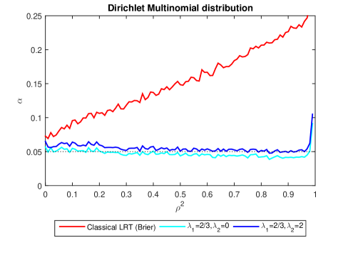
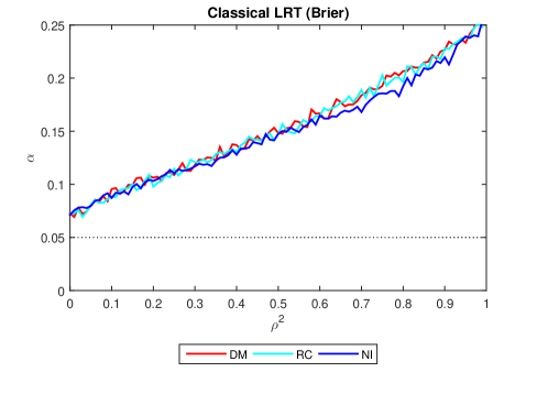
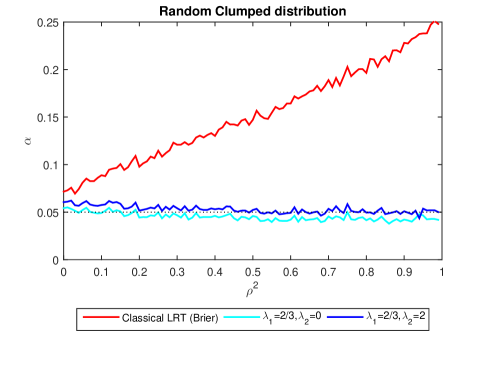
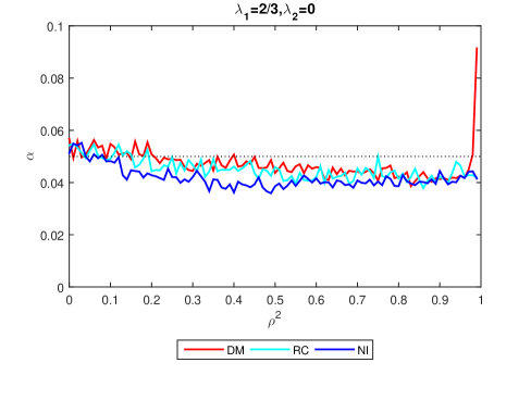
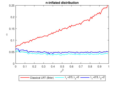
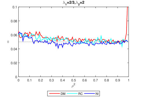
Figure 1: Estimated significance levels, by simulation, for three different distributions and types of overdispersed GOF test-statistics.

References

• [1] Alonso-Revenga, J. M., Martín, N. and Pardo, L. (2016). New improved estimators for overdispersion in models with clustered multinomial data and unequal cluster sizes. Statistics and Computing (in Press), DOI: 10.1007/s11222-015-9616-z.
• [2] Altham, P. M. E. (1976). Discrete variable analysis for individuals grouped into families. Biometrika, 63, 263–269.
• [3] Bedrick, E. J. (1983). Adjusted chi-squared tests for cross-classified tables of survey data. Biometrika, 70, 591–595.
• [4] Brier, S. S. (1980). Analysis of contingency tables under cluster sampling. Biometrika, 67, 591–596.
• [5] Choi J.W. and McHugh R.B. (1989). A reduction factor in goodness-of-fit and independence tests for clustered and weighted observations. Biometrics, 45, 979–996.
• [6] Cohen, J. E. (1976). The distribution of the chi-squared statistic under clustered sampling from contingency tables. Journal of the American Statistical Association, 71, 665–670.
• [7] Cressie, N., Pardo, L. (2002). Phi-Divergence statistics. In: ElShaarawi, A. H., Piegorich, W. W., eds. Encyclopedia of Environmetrics. Vol. 3. New York, Wiley, pp. 1551–1555.
• [8] Eldridge, S. M., Ukoumunne, O. C. and Carlin, J. B. (2009). The Intra-Cluster Correlation Coefficient in Cluster Randomized Trials: A Review of Definitions. International Statistical Review, 77, 378–394.
• [9] Fay, R. E. (1985). Complex samples. Journal of the American Statistical Association, 80, 148–157.
• [10] Fellegi, I. P. (1980). Approximate tests of independence and goodness of fit based upon stratified multistage samples. Journal of the American Statistical Association, 75, 261–268.
• [11] Fienberg, S. E. (1979). The use of chi-square statistics for categorical data problems. Journal of the Royal Statistical Society, Series B, 41, 54–64.
• [12] Holt, D., Scott, A. J. and Ewings, P. O. (1980). Chi-squared tests with survey data. Journal of the Royal Statistical Society, Series A, 143, 302–320.
• [13] Koch, G. G., Freeman, D. H., and Freeman, J. L. (1975). Strategies in the multivariate analysis of data from complex surveys. International Statistical Review, 43, 59–78.
• [14] Landis, J. R., Lepkowski, J. M., Eklund, S. A. and Stehouwer, S. A. (1984). A Statistical Methodology for Analyzing Data from a Complex Survey: The First National Health and Nutrition Examination Survey. Series 2 , No. 92. Hyattsville, Maryland: The National Center for Health Statistics.
• [15] Menéndez, M. L., Morales, D., Pardo, L. and Vajda, I. (1995). Divergence-based estimation and testing of statistical models of classification. Journal of Multivariate Analysis, 54, 329–354.
• [16] Menéndez, M. L., Morales, D., Pardo, L. and Vajda, I. (1996). About divergence-based goodness-of-fit tests in the dirichlet-multinomial model. Communications in Statistics - Theory and Methods, 25, 1119–1133.
• [17] Morel, J.G. and Nagaraj, N.K. (1993). A finite mixture distribution for modelling multinomial extra variation. Biometrika, 80, 363–371.
• [18] Mosimann, J. E. (1962). On the compound multinomial distributions, the multivariate $\beta$-distribution and correlation among proportions. Biometrika, 49, 65–82.
• [19] Pardo, L. (2006). Statistical inference based on divergence measures. Chapman & Hall/CRC, Boca Raton.
• [20] Raim, A. M. , Neerchal, N. K. and Morel, J. G. (2015). Modeling overdispersion in $R.$ Technical Report HPCI-2015-1 UMBCH High Performance Computing Facility, University of Maryland.
• [21] Rao, J. N. K. and Scott, A. J. (1981). The analysis of categorical data from complex sample surveys: Chi-squared tests for goodness of fit and independence in two-way tables. Journal of the American Statistical Association, 76, 221–230.
• [22] Rao, J. N. K. and Scott, A. J. (1984). On chi-squared tests for multiway contingency tables with cell proportions estimated from survey data. The Annals of Statistics, 12, 46–60.