Sparse Control of Multiagent Systems

Abstract

In recent years, numerous studies have focused on the mathematical modeling of social dynamics, with self-organization, i.e., the autonomous pattern formation, as the main driving concept. Usually, first or second order models are employed to reproduce, at least qualitatively, certain global patterns (such as bird flocking, milling schools of fish or queue formations in pedestrian flows, just to mention a few). It is, however, common experience that self-organization does not always spontaneously occur in a society. In this review chapter we aim to describe the limitations of decentralized controls in restoring certain desired configurations and to address the question of whether it is possible to externally and parsimoniously influence the dynamics to reach a given outcome. More specifically, we address the issue of finding the sparsest control strategy for finite agent-based models in order to lead the dynamics optimally towards a desired pattern.

1 Introduction

The autonomous formation of patterns in multiagent dynamical systems is a fascinating phenomenon which has spawned an enormous wealth of interdisciplinary studies: from social and economic networks battiston ; currarini2009economic , passing through cell aggregation and motility camazineselforganization ; kese70 ; KocWhi98 ; be07 , all the way to coordinated animal motion MR2507454 ; ChuDorMarBerCha07 ; cristiani2010modeling ; couzinlaneformation ; couzin2005N ; CS ; Niw94 ; PE99 ; ParVisGru02 ; Rom96 ; TonTu95 ; YEECBKMS09 and crowd dynamics albi2015invisible ; cristiani2011multiscale ; CucSmaZho04 ; MR2438215 . Beyond biology and sociology, the principles of self-organization in multiagent systems are employed in engineering and information science to produce cheap, resilient, and efficient squadrons of autonomous machines to perform predefined tasks arvin2014development and to render swarms of animals reynolds1987flocks and hair/fur textures in CGI animations pixarhair . The scientific literature on the subject is vast and ever-growing: the interested reader may be addressed to bak2013nature ; CCH13 ; cafotove10 ; viza12 and references therein for further insights on the topic.

A common feature of all those studies is that self-organization is the result of the superimposition of binary interactions between agents amplified by an accelerating feedback loop. This reinforcement process is necessary to give momentum to the multitude of feeble local interactions and to eventually let a global pattern appear. Typically, the strength of such interaction forces is a function of the “social distance” between agents: for instance, birds align with their closest neighbors parisi08 and people agree easier with those who already conform to their beliefs krause02 . Some of the forces of the system may be of cohesive type, i.e., they tend to reduce the distance between agents: whenever cohesive forces have a comparable strength at short and long range, we call these systems heterophilious; if, instead, there is a long-range bias we speak of homophilious societies motsch2014heterophilious . Heterophilious systems have a natural tendency to keep the trajectories of the agents inside a compact region, and therefore to exhibit stable asymptotic profiles, modeling the autonomous emergence of global patterns. On the other hand, self-organization in homophilious societies can be accomplished only conditionally to sufficiently high levels of initial coherence that allow the cohesive forces to keep the dynamics compact birdsofafeather . Being such systems ubiquitous in real life (e.g., see kirman2007marginal ), it is legitimate to ask whether – in case of lost cohesion – additional forces acting on the agents of the system may restore stability and achieve pattern formation.

A first solution to facilitate self-organization is to consider decentralized control strategies: these consist in assuming that each agent, besides being subjected to forces induced in a feedback manner by the rest of the population, follows an individual strategy to coordinate with the other agents. However, as it was clarified in bongini2015conditional , even if we allow agents to self-steer towards consensus according to additional decentralized feedback rules computed with local information, their action results in general in a minor modification of the initial homophilious model, with no improvement in terms of promoting unconditional pattern formation. Hence, blindly insisting and believing on decentralized control is certainly fascinating, but rather wishful, as it does not secure self-organization.

Such additional forces may eventually be the result of an offline optimization among perfectly informed players: in this case we fall into the realm of Game Theory nash1950equilibrium ; von2007theory . Games without an external regulator model situations where it is assumed that an automatic tendency to reach “correct” equilibria exists, like the stock market. However, also in this case such an optimistic view of the dynamics is often frustrated by evidences of the convergence to suboptimal configurations hardin1968tragedy , whence the need of an external figure controlling the evolution of the system.

For all these reasons, in the seminal papers caponigro2013sparsefake ; caponigro2015sparse external controls with limited strength were considered to promote self-organization in multiagent systems. Notice that, in such situations, efficient control strategies should target only few individuals of the population, instead of squandering resources on the entire group at once: taking advantage of the mutual dependencies between the agents, they should trigger a ripple effect that would spread their influence to the whole system, thus indirectly controlling the rest of the agents. The property of control strategies to target only a small fraction of the total population is known in the mathematical literature as sparsity tao ; donoho ; fora10 . The fundamental issue is the selection of the few agents to control: an effective criterion is to choose them as to maximize the decay rate of some Lyapunov functional associated to the stability of the desired pattern cohen1983absolute .

As a paradigmatic case study, let us consider alignment models CS ; krause02 : these are dissipative systems where imitation is the dominant feedback mechanism and in which the emerging pattern is a state where agents are fully aligned, also called consensus. For several of such models it has been proved that consensus emergence can be guaranteed regardless of the initial conditions of the system only if the alignment forces are sufficiently strong at far distance, see HaHaKim ; haskovec2014note ; in case they are not, it is easy to provide counterexamples to the emergence of a consensus. If we were to use the criterion above to select a control strategy to steer the system to consensus, it would lead to a sparse control targeting at each instant only the agent farthest away from the mean consensus parameter. Surprisingly enough, for such systems not only this strategy works for every initial condition, but the control of the instantaneous leaders of the dynamics is more convenient than controlling simultaneously all agents. Therefore if, on the one side, the homophilious character of a society plays against its compactness, on the other side, it may plays at its advantage if we allow for sparse interventions to restore consensus.

The above results have more far-reaching potential as they can be extended to non-dissipative systems as well, like the Cucker-Dong model of attraction and repulsion cucker14 . In this model, agents autonomously organize themselves in a cohesive and collision-avoiding configuration provided that the total energy is below a certain level. The sparse control strategy is able to raise this level considerably and it is optimal in maximizing the convergence of the energy functional towards it. However in this case, due to the singular non-conservative forces in play, it may be seen that sparse controllability is in general conditional to the choice of the initial conditions, as opposed to the unconditional controllability of alignment models.

The essential scope of this review chapter is to describe in more detail the aforementioned mechanisms relating sparse controllability and pattern formation. We do so by condensing the results of the papers bofo13 ; bongini2014sparse ; bongini2015conditional ; caponigro2015sparse , addressing the limitations of decentralized control strategies, the sparse controllability of alignment models and the one of attraction repulsion models.

2 Self-organization in dynamical communication networks

We start from the analysis of general properties of alignment models. Instances of these models are ubiquitous in nature since several species are able to interpret and instinctively reproduce certain manoeuvres that they perceive (e.g., fleeing from a danger, searching for food, performing defense tactics, etc.), see animalbehavior . Such systems may be seen as networks of agents with oriented information flow under possible link failure or creation, and can be effectively represented by means of directed graphs with edges possibly switching in time.

A directed graph $G$ on a set of nodes $A_{1},\ldots,A_{N}$ is any subset of $\{A_{1},\ldots,A_{N}\}^{2}$. Each pair $(A,B)\in G$ is called an edge from $A$ to $B$, and a directed path from $A$ to $B$ in $G$ is a sequence of edges $(A,A_{i_{1}}),(A_{i_{1}},A_{i_{2}}),\ldots,(A_{i_{k}},B)\in G$. The graph $G$ is said to be strongly connected if for any pair $A,B$ of distinct nodes there is a directed path from $A$ to $B$ and a directed path from $B$ to $A$.

When studying under which conditions networks of agents are able to self-organize, it is usually not enough to know if two nodes are connected: the strength of the interaction between them also matters. Hence, given a system of $N\in{\mathbb{N}}$ agents, for each pair of agents $i,j=1,\ldots,N$ we denote by $g_{ij}(t)\in{\mathbb{R}}_{+}$ the weight of the link connecting $i$ with $j$: clearly, if $g_{ij}(t)=0$, $i$ is not connected to $j$ at time $t$. The value $g_{ij}(t)$ can be seen as the relative intensity of the information exchange flowing from agent $i$ to agent $j$ at time $t\geq 0$. We shall assume for the moment that each weight function $g_{ij}:{\mathbb{R}}_{+}\rightarrow{\mathbb{R}}_{+}$ is piecewise continuous.

The weights $g_{ij}(\cdot)$ naturally induce a directed graph structure on the set of agents: we define, for any $\varepsilon\geq 0$ and $t\geq 0$, the graph $G_{\varepsilon}(t)$ as

$$G_{\varepsilon}(t)\stackrel{{\scriptstyle\Delta}}{{=}}\left\{{(i,j)\in\{1,\ldots,N\}^{2}}:{g_{ij}(t)>\varepsilon}\right\}.$$

The adjacency matrix $G_{0}(t)$ is the set of pairs $(i,j)$ for which the communication channel from $i$ to $j$ is active at time $t$.

As a prototypical example of a multiagent system and to quantitatively illustrate the concept of self-organization, we introduce alignment models: if we denote by $\{v_{1},\ldots,v_{N}\}\subset{\mathbb{R}}^{d}$ the states of the $N$ agents of our systems, then the instantaneous evolution of the state $v_{i}(t)$ of agent $i$ at time $t$ is given by

$$\dot{v}_{i}(t)=\sum^{N}_{j=1}g_{ij}(t)(v_{j}(t)-v_{i}(t)),\quad i=1,\ldots,N.$$ (1)

The meaning of the above system of differential equations is the following: at each instant $t\geq 0$, the state $v_{i}(t)$ of agent $i$ tends to the state $v_{j}(t)$ of agent $j$ with a speed that depends on the strength of the information exchange $g_{ij}(t)$. Since (1) is a system of ODEs with possibly discontinuous coefficients, we need for it a proper notion of solution.

Definition 1

Let $\{I_{k}\}_{k\in{\mathbb{N}}}$ denote a countable family of open intervals such that all the functions $g_{ij}$ are continuous on every $I_{k}$ and $\cup_{k\in{\mathbb{N}}}\overline{I}_{k}={\mathbb{R}}_{+}$. Given $v^{0}=(v^{0}_{1},\ldots,v^{0}_{N})\in{\mathbb{R}}^{dN}$, we say that the curve $v=(v_{1},\ldots,v_{N}):{\mathbb{R}}_{+}\rightarrow{\mathbb{R}}^{dN}$ is a solution of (1) with initial datum $v^{0}$ if

1. $v(0)=v^{0}$;

2. for every $i=1,\ldots,N$ and $k\in{\mathbb{N}}$, $v_{i}$ satisfies (1) on $I_{k}$.

The notion of self-organization that we are considering for system (1) is that of consensus or flocking, which is the situation where the state variables of the agents asymptotically coincide.

Definition 2 (Consensus for system (1))

Let $v:{\mathbb{R}}_{+}\rightarrow{\mathbb{R}}^{dN}$ denote a solution of (1) with initial datum $v^{0}$. We say that $v(\cdot)$ converges to consensus if there exists a $v^{\infty}\in{\mathbb{R}}^{d}$ such that, for every $i=1,\ldots,N$, it holds

$$\lim_{t\rightarrow+\infty}\|v_{i}(t)-v^{\infty}\|_{\ell^{d}_{2}}=0.$$

The value $v^{\infty}$ is called the consensus state.

In the definition above, $\|\cdot\|_{\ell^{d}_{2}}$ stands for the Euclidean norm on ${\mathbb{R}}^{d}$. The subscript $\ell^{d}_{2}$ shall often be omitted whenever clear from context.

Roughly speaking, a system of agents satisfying (1) converges to consensus regardless of the initial condition $v^{0}$ provided that the underlying communication graph is “sufficiently connected”. With this we mean that each node must possess, over some dense collection of time intervals, a strong enough communication path to every other node in the network. This intuitive idea is made precise in the following result, whose proof can be found in haskovec2014note . A similar answer for discrete-time systems was also provided in moreau2005stability

Theorem 2.1

Let $v:{\mathbb{R}}_{+}\rightarrow{\mathbb{R}}^{dN}$ be a solution of (1) with initial datum $v^{0}$. Suppose that there exists an $\varepsilon>0$ and a strongly connected directed graph $G$ on the set of agents on which the system spends an infinite amount of time, i.e.,

$$\mathcal{L}^{1}\left({\left\{{t\geq 0}:{G_{\varepsilon}(t)=G}\right\}}\right)=+\infty.$$

Then $v(\cdot)$ converges to consensus with consensus state $v^{\infty}$ belonging to the convex hull of $\{v^{0}_{1},\ldots,v^{0}_{N}\}$.

The above result is closely related, for instance, to (motsch2014heterophilious, , Theorem 2.3), which requires a stronger connectivity of the network of agents (the quantity $\eta_{A}$ in (motsch2014heterophilious, , Equation (2.5))) but also gives an explicit rate for the convergence towards $v^{\infty}$ (see (motsch2014heterophilious, , Equation (2.6b))).

Theorem 2.1 also says that, without further hypotheses on the interaction weights $g_{ij}$, the value of $v^{\infty}$ is rather an emergent property of the global dynamics of system (1) than a mere function of the initial datum $v^{0}$. Nonetheless, it is relatively simple to identify assumptions on $g_{ij}$ for which the latter is true. For example, from a trivial computation follows

$$\frac{1}{N}\sum^{N}_{i=1}\dot{v}_{i}(t)=\frac{1}{N}\sum^{N}_{j=1}\left(\sum^{N}_{i=1}g_{ij}(t)-\sum^{N}_{i=1}g_{ji}(t)\right)v_{j}(t).$$

Hence, if for every $t\geq 0$ the weight matrix $(g_{ij}(t))_{i,j=1}^{N}$ has the property that $\sum^{N}_{i=1}g_{ij}(t)=\sum^{N}_{i=1}g_{ji}(t)$ for every $j=1,\ldots,N$, then the average

$$\overline{v}(t)\stackrel{{\scriptstyle\Delta}}{{=}}\frac{1}{N}\sum^{N}_{i=1}v_{i}(t)$$ (2)

is an invariant of the dynamics. This implies that $v^{\infty}=\overline{v}(0)$ holds, i.e., the consensus state is only a function of the initial datum $v^{0}$.

3 Consensus emergence in alignment models

In this section we shall see that the assumptions of Theorem 2.1 can actually be very restrictive and seldom met when dealing with specific instances of alignment models.

3.1 Some classic examples of alignment models

A general principle in opinion formation is the conformity bias, i.e., agents weight more opinions that already conform to their beliefs. This can, actually, be extended to coordination in general, since intuitively it is easier to coordinate with “near” agents than “far away” ones. Formally, this is equivalent to asking that the weights $g_{ij}$ are a nonincreasing function of the distance between the states of the agents, i.e.,

$$g_{ij}(t)=a(\|v_{i}(t)-v_{j}(t)\|),$$ (3)

where $a:{\mathbb{R}}_{+}\rightarrow{\mathbb{R}}_{+}$ is a nonincreasing interaction kernel. Notice that (3) trivially implies the invariance of the mean $\overline{v}$ (given by (2)), and that $v^{\infty}=\overline{v}(0)$, if it exists.

Several classic opinion formation models combine conformity bias with alignment. In the DW model, see weisbuch , two random agents $i$ and $j$ update their opinions $v_{i}$ and $v_{j}$ to $1/2(v_{i}+v_{j})$, provided they originally satisfy $\|v_{i}-v_{j}\|\leq R$, where $R>0$ is fixed a priori. Instead, in the popular bounded confidence model of Hegselmann and Krause krause02 , opinions evolves according to the dynamics (1) where the function $a$ has the form

$$a(r)=\chi_{[0,R]}(r)\stackrel{{\scriptstyle\Delta}}{{=}}\begin{cases}1&\text{ if }r\in[0,R],\\ 0&\text{ otherwise,}\\ \end{cases}$$

for some fixed confidence radius $R>0$. The dynamics is thus given by the system of ODEs

$$\dot{v}_{i}(t)=\frac{1}{|\Lambda_{R}(t,i)|}\sum^{N}_{j=1}\chi_{[0,R]}(\|v_{i}(t)-v_{j}(t)\|)(v_{j}(t)-v_{i}(t)),\quad i=1,\ldots,N,$$ (4)

where we have set

$$\Lambda_{R}(t,i)\stackrel{{\scriptstyle\Delta}}{{=}}\left\{{j\in\{1,\ldots,N\}}:{\|x_{i}(t)-x_{j}(t)\|\leq R}\right\},$$ (5)

and $|\Lambda_{R}(t,i)|$ stands for its cardinality. It is straightforward to design an instance of this model not fulfilling the hypothesis of Theorem 2.1. Indeed, consider a group of $N=2$ agents in dimension $d=1$ with initial conditions $v_{1}(0)=-R$ and $v_{2}(0)=R$. Since $g_{12}(0)=g_{21}(0)=0$, it follows that $G_{\varepsilon}(t)=\emptyset$ for all $t\geq 0$ and for all $\varepsilon\geq 0$.

Second-order models are necessary whenever we want to describe the dynamics of physical agents, like flocks of birds, herds of quadrupeds, schools of fish, and colonies of bacteria, where individuals are considered aligned whenever they move in the same direction, regardless of their position. Since in such cases it is necessary to perceive the velocities of the others in order to align, to describe the motion of the agents we need the pair position-velocity $(x,v)$, but this time only the velocity variable $v$ is the consensus parameter.

One of the first of such models, named Vicsek’s model in honor of one of its fathers, was introduced in vicsek1995novel . Very much in the spirit of (4), it postulates that the evolution of the spatial coordinate $x_{i}$ and of the orientation $\theta_{i}\in[0,2\pi]$ in the plane ${\mathbb{R}}^{2}$ of the $i$-th agent follows the law of motion given by

$$\left\{\begin{aligned} \hfil\displaystyle\begin{split}\dot{x}_{i}(t)&=v_{i}(t)=\hat{v}\left(\begin{matrix}\cos(\theta_{i}(t))\\ \sin(\theta_{i}(t))\end{matrix}\right),\\ \dot{\theta}_{i}(t)&=\frac{1}{|\Lambda_{R}(t,i)|}\sum_{j=1}^{N}\chi_{[0,R]}\left(\|x_{i}(t)-x_{j}(t)\|\right)\left(\theta_{j}(t)-\theta_{i}(t)\right),\end{split}\quad i=1,\ldots,N,\end{aligned}\right.$$ (6)

where $\hat{v}>0$ denotes the constant modulus of $v_{i}(t)$.In this model, the orientation of the consensus parameter $v_{i}$ is adjusted with respect to the other agents according to a weighted average of the differences $\theta_{j}-\theta_{i}$. The influence of the $j$-th agent on the dynamics of the $i$-th one is a function of the (physical or social) distance between the two agents: if this distance is less than $R$, the agents interact by appearing in the computation of the respective future orientation.

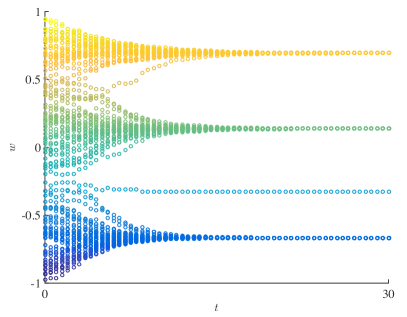
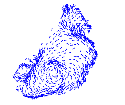
Figure 1: On the left: a typical evolution of the Hegselmann-Krause model. On the right: mill patterns in the Vicsek model. (Kind courtesy of G. Albi)

In CS , the authors proposed a possible extension of system (6) to dimensions $d>2$ as follows

$$\left\{\begin{aligned} \hfil\displaystyle\begin{split}\dot{x}_{i}(t)&=v_{i}(t),\\ \dot{v}_{i}(t)&=\frac{1}{|\Lambda_{R}(t,i)|}\sum_{j=1}^{N}\chi_{[0,R]}\left(\|x_{i}(t)-x_{j}(t)\|\right)\left(v_{j}(t)-v_{i}(t)\right),\end{split}\qquad i=1,\ldots,N.\end{aligned}\right.$$

The substitution of the function $\chi_{[0,R]}$ with a strictly positive kernel $a:{\mathbb{R}}_{+}\rightarrow{\mathbb{R}}_{+}$ let us drop the highly irregular and nonsymmetric normalizing factor $|\Lambda_{R}(t,i)|$ in favor of a simple $N$, and leads to the system

$$\left\{\begin{aligned} \hfil\displaystyle\begin{split}\dot{x}_{i}(t)&=v_{i}(t),\\ \dot{v}_{i}(t)&=\frac{1}{N}\sum_{j=1}^{N}a\left(\|x_{i}(t)-x_{j}(t)\|\right)\left(v_{j}(t)-v_{i}(t)\right),\end{split}\qquad i=1,\ldots,N.\end{aligned}\right.$$ (7)

Notice that the equation governing the evolution of $v_{i}$ has the same form as (1), and since now the weights $g_{ij}$ are symmetric (i.e., $g_{ij}=g_{ji}$ for all $i,j=1,\ldots,N$) then $\overline{v}$ is a conserved quantity.

An example of a system of the form (7) is the influential model of Cucker and Smale, introduced in CS , in which the function $a$ is

$$a(r)\stackrel{{\scriptstyle\Delta}}{{=}}\frac{H}{(\sigma^{2}+r^{2})^{\beta}},$$ (8)

where $H>0$, $\sigma>0$, and $\beta\geq 0$ are constants accounting for the social properties of the group. Systems like (7) are usually referred to as Cucker-Smale systems due to the influence of their work, as can be witnessed by the wealth of literature focusing on their model, see for instance ahn2010stochastic ; carrillo2010asymptotic ; dalmao2011cucker ; ha2009simple ; perea2009extension ; shen2007cucker .

3.2 Pattern formation for the Cucker-Smale model

We now focus on consensus emergence for system (7). In the following, we shall consider a kernel $a:{\mathbb{R}}_{+}\rightarrow{\mathbb{R}}_{+}$ which is decreasing, strictly positive, bounded and Lipschitz continuous.

As already noticed, in second-order models alignment means that all agents move with the same velocity, but not necessarily are in the same position. Therefore, Definition 2 of consensus applies here on the $v_{i}$ variables only.

Definition 3 (Consensus for system (7))

We say that a solution

$$(x,v)=(x_{1},\ldots,x_{N},v_{1},\ldots,v_{N}):{\mathbb{R}}_{+}\rightarrow{\mathbb{R}}^{2dN}$$

of system (7) tends to consensus if the consensus parameter vectors $v_{i}$ tend to the mean $\overline{v}$, i.e.,

$$\lim_{t\rightarrow+\infty}\left\|{v_{i}(t)-\overline{v}(t)}\right\|=0\quad\text{for every }i=1,\ldots,N.$$

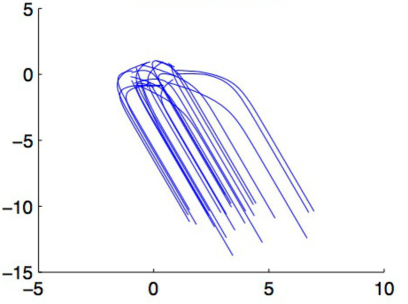
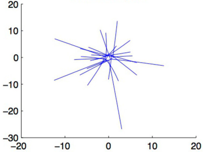
Figure 2: Consensus behavior of a Cucker-Smale system. On the left: agents align with the mean velocity. On the right: agents fail to reach consensus.

The following result is an easy corollary of Theorem 2.1.

Corollary 1

Let $(x(\cdot),v(\cdot))$ be a solution of system (7), where the interaction kernel $a$ is decreasing and strictly positive. Suppose that there exists $R>0$ for which it holds

$$\mathcal{L}^{1}\left({\left\{{t\geq 0}:{\left\|{x_{i}(t)-x_{j}(t)}\right\|\leq R\;\text{ for all }\;i,j=1,\ldots,N}\right\}}\right)=+\infty.$$

Then $(x(\cdot),v(\cdot))$ converges to consensus.

Proof

Since $a$ is decreasing and strictly positive, from the initial assumptions follows

$$g_{ij}(t)=\frac{1}{N}a(\left\|{x_{i}(t)-x_{j}(t)}\right\|)\geq\frac{a(R)}{N}>0,$$

for every $t\geq 0$ for which $\left\|{x_{i}(t)-x_{j}(t)}\right\|\leq R$ holds for every $i,j=1,\ldots,N$. Therefore, the condition $\left\|{x_{i}(t)-x_{j}(t)}\right\|\leq R$ for every $i,j=1,\ldots,N$ implies $G_{a(R)/N}(t)=\{1,\ldots,N\}^{2},$ which yields

$$\mathcal{L}^{1}\left({\left\{{t\geq 0}:{G_{a(R)/N}(t)=\{1,\ldots,N\}^{2}}\right\}}\right)=+\infty,$$

The statement then follows from Theorem 2.1 for the choice $\varepsilon=a(R)/N$.

Unfortunately, the result above has the serious flaw that it cannot be invoked directly to infer convergence to consensus, since establishing a uniform bound in time for the distances of the agents is very difficult, even for smooth kernels like (8). Intuitively, consider the case where the interaction strength is too weak and the agents too dispersed in space to let the velocities $v_{i}$ align. In this case, nothing prevents the distances $\|x_{i}-x_{j}\|$ to grow indefinitely, violating the hypothesis of Corollary 1. Hence, in order to obtain more satisfactory consensus results, we need to follow approaches that take into account the extra information at our disposal, which are the strength of the interaction and the initial configuration of the system.

Originally, this problem was studied in CS ; cusm07 borrowing several tools from Spectral Graph Theory, see as a reference chung1997spectral . Indeed, system (7) can be rewritten in the following compact form

$$\left\{\begin{aligned} \dot{x}(t)&=v(t),\\ \dot{v}(t)&=L(x(t))v(t),\end{aligned}\right.$$ (9)

where $L(x(t))$ is the Laplacian of the matrix $(a\left(\left\|{x_{i}(t)-x_{j}(t)}\right\|\right)/N)_{i,j=1}^{N}$, which is a function of $x(t)$. Being the Laplacian of a positive definite, symmetric matrix, $L(x(t))$ encodes plenty of information regarding the adjacency matrix $G_{0}(t)$ of the system, see mohar1991laplacian . In particular, the second smallest eigenvalue $\lambda_{2}(t)$ of $L(x(t))$, called the Fiedler’s number of $G_{0}(t)$ is deeply linked with consensus emergence: provided that a sufficiently strong bound from below of $\lambda_{2}(t)$ is available, the system converges to consensus.

To establish under which conditions we have convergence to consensus, we shall follow a different approach. The advantage of it is that it can be employed also to study the issue of the controllability of several multiagent systems (see Section 5).

3.3 The consensus region

A natural strategy to improve Corollary 1 would be to look for quantities which are invariant with respect to $\overline{v}$, since it is conserved in systems like (7).

Definition 4

The symmetric bilinear form $B:{\mathbb{R}}^{dN}\times{\mathbb{R}}^{dN}\rightarrow{\mathbb{R}}$ is defined, for any $v,w\in{\mathbb{R}}^{dN}$, as

$$B(v,w)\stackrel{{\scriptstyle\Delta}}{{=}}\frac{1}{2N^{2}}\sum^{N}_{i=1}\sum^{N}_{j=1}(v_{i}-v_{j})\cdot(w_{i}-w_{j}),$$

where $\cdot$ denotes the usual scalar product on ${\mathbb{R}}^{d}$.

Remark 1

It is trivial to prove that

$$B(v,w)=\frac{1}{N}\sum^{N}_{i=1}(v_{i}\cdot w_{i})-\overline{v}\cdot\overline{w},$$ (10)

where $\overline{v}$ stands for the average of the elements of the vector $v=(v_{1},\ldots,v_{N})$ given by (2). From this representation of $B$ follows easily that the two spaces

$$\mathcal{V}_{f} \stackrel{{\scriptstyle\Delta}}{{=}}\left\{{v\in{\mathbb{R}}^{dN}}:{v_{1}=\ldots=v_{N}}\right\}\quad\text{and}\quad\mathcal{V}_{\perp}\stackrel{{\scriptstyle\Delta}}{{=}}\left\{{v\in{\mathbb{R}}^{dN}}:{\sum^{N}_{i=1}v_{i}=0}\right\},$$

are perpendicular with respect to the scalar product $B$, i.e., ${\mathbb{R}}^{dN}=\mathcal{V}_{f}\oplus\mathcal{V}_{\perp}$. This means that every $v\in{\mathbb{R}}^{dN}$ can be written uniquely as $v=v^{f}+v^{\perp}$, where $v^{f}\in\mathcal{V}_{f}$ and $v^{\perp}\in\mathcal{V}_{\perp}$. A closer inspection reveals that it holds $v^{f}_{i}=\overline{v}$ and $v^{\perp}_{i}=v_{i}-\overline{v}$ for every $i=1,\ldots,N$. Notice that, since $v^{\perp}\in\mathcal{V}_{\perp}$, for any vector $w\in{\mathbb{R}}^{d}$ it holds

$$\sum^{N}_{i=1}(v^{\perp}_{i}\cdot w)=\left(\sum^{N}_{i=1}v^{\perp}_{i}\right)\cdot w=0.$$ (11)

Since for every $v,w\in{\mathbb{R}}^{dN}$ we have $B(v^{f},w)=0=B(v,w^{f})$, it holds

$$B(v,w)=B(v^{\perp},w)=B(v,w^{\perp})=B(v^{\perp},w^{\perp}).$$

This means that $B$ distinguishes two vectors modulo their projection on $\mathcal{V}_{f}$. Moreover, from (10) immediately follows that $B$ restricted to $\mathcal{V}_{\perp}\times\mathcal{V}_{\perp}$ coincides, up to a factor $1/N$, with the usual scalar product on ${\mathbb{R}}^{dN}$.

Remark 2 (Consensus manifold)

Notice that whenever the initial datum $(x^{0},v^{0})$ belongs to the set ${\mathbb{R}}^{dN}\times\mathcal{V}_{f}$, the right-hand size of $\dot{v}_{i}$ in (7) is 0, hence the equality $v_{1}(t)=\ldots=v_{N}(t)$ is satisfied for all $t\geq 0$ and the system is already in consensus. For this reason, the set ${\mathbb{R}}^{dN}\times\mathcal{V}_{f}$ is called the consensus manifold.

The bilinear form $B$ can be used to characterize consensus emergence for solutions $(x(\cdot),v(\cdot))$ of system (7) by setting

$$X(t)\stackrel{{\scriptstyle\Delta}}{{=}}B(x(t),x(t))\quad\text{ and }\quad V(t)\stackrel{{\scriptstyle\Delta}}{{=}}B(v(t),v(t)).$$

The functionals $X$ and $V$ provide a description of consensus by measuring the spread, both in positions and velocities, of the trajectories of the solution $(x(\cdot),v(\cdot))$, as the following trivial result shows.

Proposition 1

The following statements are equivalent:

1. $\lim_{t\rightarrow+\infty}\left\|{v_{i}(t)-\overline{v}(t)}\right\|=0$ for every $i=1,\ldots,N$;

2. $\lim_{t\rightarrow+\infty}v_{i}^{\perp}(t)=0$ for every $i=1,\ldots,N$;

3. $\lim_{t\rightarrow+\infty}V(t)=0$.

The following Lemma shows that $V$ is a Lyapunov functional for system (7).

Lemma 1 ((caponigro2015sparse, , Lemma 1))

Let $(x(\cdot),v(\cdot))$ be a solution of system (7). Then for every $t\geq 0$ it holds

$$\frac{d}{dt}V(t)\leq-2a(\sqrt{2NX(t)})V(t).$$ (12)

Therefore, $V$ is decreasing.

By means of the quantities $X$ and $V$ we can provide a sufficient condition for consensus emergence for solutions of system (7).

Theorem 3.1 ((HaHaKim, , Theorem 3.1))

Let $(x^{0},v^{0})\in{\mathbb{R}}^{dN}\times{\mathbb{R}}^{dN}$ and set $X_{0}\stackrel{{\scriptstyle\Delta}}{{=}}B(x^{0},x^{0})$ and $V_{0}\stackrel{{\scriptstyle\Delta}}{{=}}B(v^{0},v^{0})$. If the following inequality is satisfied

$$\int^{+\infty}_{\sqrt{X_{0}}}a(\sqrt{2N}r)\ dr\geq\sqrt{V_{0}},$$ (13)

then the solution of (7) with initial datum $(x^{0},v^{0})$ tends to consensus.

The inequality (13) defines a region in the space $(X_{0},V_{0})$ of initial conditions for which the balance between $X_{0}$, $V_{0}$ and the kernel $a$ is such that the system tends to consensus autonomously.

Definition 5 (Consensus region)

We call consensus region the set of points $(X_{0},V_{0})\in{\mathbb{R}}^{dN}\times{\mathbb{R}}^{dN}$ satisfying (13).

The size of the consensus region gives an estimate of how large the basin of attraction of the consensus manifold ${\mathbb{R}}^{dN}\times\mathcal{V}_{f}$ is. If the rate of communication function $a$ is integrable, i.e., far distant agents are only weakly influencing the dynamics, then such a region is essentially bounded, and actually not all initial conditions will realize self-organization, as the following example shows.

Example 1 ((CS, , Proposition 5))

Consider $N=2$ agents in dimension $d=1$ subject to system (7) with interaction kernel given by (8) with $H=1/2$, $\sigma=1$, and $\beta=1$. If we denote by $(x_{1}(\cdot),v_{1}(\cdot))$ and $(x_{2}(\cdot),v_{2}(\cdot))$ the trajectories of the two agents, it is easy to show that the evolution of the relative main state $x(t)\stackrel{{\scriptstyle\Delta}}{{=}}x_{1}(t)-x_{2}(t)$ and of the relative consensus state $v(t)\stackrel{{\scriptstyle\Delta}}{{=}}v_{1}(t)-v_{2}(t)$ is given for every $t\geq 0$ by

$$\left\{\begin{aligned} \hfil\displaystyle\begin{split}\dot{x}(t)&=v(t),\\ \dot{v}(t)&=-\frac{v(t)}{1+x(t)^{2}},\end{split}\end{aligned}\right.$$ (14)

with initial condition $x(0)=x^{0}$ and $v(0)=v^{0}$ (without loss of generality, we may assume that $x^{0},v^{0}>0$). An explicit solution of the above system can be easily derived by means of direct integration:

$$v(t)-v^{0}=-\arctan x(t)+\arctan x^{0}.$$

Condition (13) in this case reads $\pi/2-\arctan x^{0}\geq v^{0}.$ Hence, suppose (13) is violated, i.e., $\arctan x^{0}+v^{0}>\pi/2$. This means $\arctan x^{0}+v^{0}\geq\pi/2+\varepsilon$ for some $\varepsilon>0$, which implies

$$|v(t)|=|-\arctan x(t)+\arctan x^{0}+v^{0}|\geq\left|-\arctan x(t)+\frac{\pi}{2}+\varepsilon\right|>\varepsilon$$

for every $t\geq 0$. Therefore, the solution of system (14) with initial datum $(x^{0},v^{0})$ satisfying $\arctan x^{0}+v^{0}>\pi/2$ does not converge to consensus, since otherwise we would have $v(t)\rightarrow 0$ for $t\rightarrow+\infty$.

Remark 3

Notice that, if $\int_{\delta}^{+\infty}a(r)dr$ diverges for every $\delta\geq 0$, then the consensus region coincides with the entire space ${\mathbb{R}}^{dN}\times{\mathbb{R}}^{dN}$. In other words, in this case the interaction force between the agents is so strong that the system will reach consensus no matter what the initial conditions are.

As the following example shows, there may be initial configurations from which the system can reach consensus automatically even if condition (13) is not satisfied.

Example 2

Consider an instance of the Cucker-Smale system (7) without control in dimension $d=1$ with $N=2$ agents, where the interaction function $a:{\mathbb{R}}_{+}\rightarrow{\mathbb{R}}_{+}$ is of the form

$$a(r)=\begin{cases}M&\text{ if }r\leq R,\\ f(r)&\text{ if }r\geq R,\end{cases}$$

for some given $R>0$ and $f:{\mathbb{R}}_{+}\rightarrow{\mathbb{R}}_{+}$ positive continuous function satisfying

$$f(R)=M\quad\text{ and }\quad\int^{+\infty}_{R}f(r)\,dr=\varepsilon<+\infty.$$

The constant $M>0$ is to be properly chosen later on. Assume that the initial state and consensus parameters of the two agents are $(x^{0}_{1},v^{0}_{1})=(-R/2,v^{0})$ and $(x^{0}_{2},v^{0}_{2})=(R/2,-v^{0})$ respectively, for some $v^{0}>\varepsilon/2$.

Due to the nature of the situation, is fairly easy to check if condition (13) of Theorem 3.1 is satisfied or not. Indeed we have $X(0)=R^{2}/4$ and $V(0)=(v^{0})^{2}$, and, by the particular form of $a$, after a change of variables the computation below follows

$$\int^{+\infty}_{\frac{R}{2}}a(2r)\,dr=\frac{1}{2}\int^{+\infty}_{R}a(r)\,dr=\frac{1}{2}\int^{+\infty}_{R}f(r)\,dr=\frac{\varepsilon}{2}.$$

Therefore at time $t=0$ we are not in the consensus region given by (13), since

$$\int^{+\infty}_{\sqrt{X(0)}}a(\sqrt{4}r)\,dr=\frac{\varepsilon}{2}<v^{0}=\sqrt{V(0)}.$$

We now show that there exists a time $T>0$ such that

$$\int^{+\infty}_{\sqrt{X(T)}}a(\sqrt{4}r)\,dr\geq\sqrt{V(T)},$$ (15)

i.e., the system enters the consensus region autonomously at time $T$.

To do so, we first compute a lower bound for the integral. Notice that, since we are considering a Cucker-Smale system with mean consensus parameter $\overline{v}=0$, the speeds $|v_{1}(t)|$ and $|v_{2}(t)|$ are decreasing by Lemma 1. Therefore, we can estimate from above the time until $|x_{1}(t)-x_{2}(t)|\leq R$ holds by $T^{*}\stackrel{{\scriptstyle\Delta}}{{=}}R/2v^{0}$ (since the agents are moving on the real line in opposite directions). Hence $X(t)\leq X(0)=R^{2}/4$ for every $t\in[0,T^{*}]$, which yields the following lower bound

$$\int^{+\infty}_{\sqrt{X(t)}}a(\sqrt{4}r)\,dr\geq\int^{+\infty}_{\sqrt{X(0)}}a(\sqrt{4}r)\,dr=\frac{\varepsilon}{2}$$

valid for any $t\leq T^{*}$.

We now compute an upper bound for the functional $\sqrt{V(t)}$ for $t\in[0,T^{*}]$. Notice that

$$a(\sqrt{4X(t)})\geq a(\sqrt{4X(0)})=a(R)=M,$$

hence by (12) we have

$$\frac{d}{dt}V(t)\leq-2MV(t)$$

which, by integration, implies that $\sqrt{V(t)}\leq v^{0}e^{-Mt}$ for every $t\in[0,T^{*}]$.

We now plug together the two bounds. In order for (15) to hold at some time $T<T^{*}$, simply choose

$$M=M_{T}\stackrel{{\scriptstyle\Delta}}{{=}}\frac{1}{T}\log\left(\frac{2v^{0}}{\varepsilon}\right).$$

For this choice of $M$, it follows

$$\int^{+\infty}_{\sqrt{X(T)}}a(\sqrt{4}r)\,dr\geq\frac{\varepsilon}{2}=v^{0}e^{-M_{T}T}\geq\sqrt{V(T)}.$$

From Theorem 3.1 we can then conclude that any solution of the above system tends autonomously to consensus.

4 The effect of perturbations on consensus emergence

An immediate way to enhance the alignment capabilities of systems like (7) consists in adding a feedback term penalizing the distance of each agent’s velocity from the average one, i.e.,

$$\left\{\begin{aligned} \hfil\displaystyle\begin{split}\dot{x}_{i}(t)&=v_{i}(t),\\ \dot{v}_{i}(t)&=\frac{1}{N}\sum_{j=1}^{N}a\left(\left\|{x_{i}(t)-x_{j}(t)}\right\|\right)\left(v_{j}(t)-v_{i}(t)\right)+\gamma(\overline{v}(t)-v_{i}(t)),\end{split}\end{aligned}\right.$$ (16)

where $\gamma>0$ is a prescribed constant, modeling the strength of the additional alignment term.

This approach to the enforcement of consensus is a particular instance of what in the literature is known as decentralized control strategy, which has been thoroughly studied especially for its application in the self-organization of unmanned aerial vehicles (UAVs) fax2004information , congestion control in communication networks paganini2001scalable , and distributed sensor newtorks cortes2005coordination . We also refer to tanner2007flocking for the stability analysis of a decentralized coordination method for dynamical systems with switching underlying communication network.

As system (16) can be rewritten as (7) with the interaction kernel $a(\cdot)+\gamma$ replacing $a(\cdot)$, by Theorem 3.1 and Remark 3 each solution of (16) tends to consensus.

However, the apparently innocent fix of adding the extra term above has actually a huge impact on the interpretation of the model: as pointed out in caponigro2015sparse , this approach requires that each agent must possess at every instant a perfect information of the whole system, since it has to correctly compute the mean velocity of the group $\overline{v}$ in order to compute its trajectory. This condition is seldom met in real-life situations, where it is usually only possible to ask that each agent computes an approximated mean velocity vector $\overline{v}_{i}$, instead of the true $\overline{v}$. These considerations lead us to the model

$$\left\{\begin{aligned} \hfil\displaystyle\begin{split}\dot{x}_{i}(t)&=v_{i}(t),\\ \dot{v}_{i}(t)&=\frac{1}{N}\sum_{j=1}^{N}a\left(\left\|{x_{i}(t)-x_{j}(t)}\right\|\right)\left(v_{j}(t)-v_{i}(t)\right)+\gamma(\overline{v}_{i}(t)-v_{i}(t)).\end{split}\end{aligned}\right.$$ (17)

In studying under which conditions the solutions of system (17) tend to consensus, it is often desirable to express the approximated feedback as a combination of a term consisting on a true information feedback, i.e., a feedback based on the real average $\overline{v}$, and a perturbation term, which models the deviation of $\overline{v}_{i}$ from $\overline{v}$. To this end, we rewrite system (17) in the following form:

$$\left\{\begin{aligned} \hfil\displaystyle\begin{split}\dot{x}_{i}(t)&=v_{i}(t),\\ \dot{v}_{i}(t)&=\frac{1}{N}\sum_{j=1}^{N}a\left(\left\|{x_{i}(t)-x_{j}(t)}\right\|\right)\left(v_{j}(t)-v_{i}(t)\right)+\alpha(t)(\overline{v}(t)-v_{i}(t))+\beta(t)\Delta_{i}(t),\end{split}\end{aligned}\right.$$ (18)

where $\alpha(\cdot)$ and $\beta(\cdot)$ are two nonnegative, piecewise continuous functions, and $\Delta_{i}(\cdot)$ is the deviation acting on the estimate of $\overline{v}$ by agent $i$ (which can, of course, depend on $(x_{1}(t),\ldots,x_{N}(t),v_{1}(t),\ldots,v_{N}(t))$). Therefore, solutions in this context have to be understood in terms of weak solutions in the Carathéodory sense, see filipov .

Remark 4

In what follows, we will not be interested in the well-posedness of system (18), but rather in finding assumptions on the functions $a$, $\alpha$, $\beta$, and $\Delta_{i}$ for which we can guarantee its asymptotic convergence to consensus.

System (18) provides the advantage of encompassing all the previously introduced models, as can be readily seen:

• if $\alpha=\beta\equiv\gamma$ and $\Delta_{i}=v_{i}-\overline{v}$, or $\alpha=\beta\equiv 0$, then we recover system (7),

• the choices $\alpha\equiv\gamma$, $\Delta_{i}\equiv 0$ (or equivalently $\beta\equiv 0$) yield system (16),

• if $\alpha=\beta\equiv\gamma$ and $\Delta_{i}=\overline{v}_{i}-\overline{v}$ we obtain system (17).

The introduction of the perturbation term in system (18) may deeply modify the nature of the original model: for instance, an immediate consequence is that the mean velocity of the system is, in general, no longer a conserved quantity.

Proposition 2

For system (18), with perturbations given by the vector-valued function $\Delta(\cdot)=(\Delta_{1}(\cdot),\ldots,\Delta_{N}(\cdot))$, for every $t\geq 0$ it holds

$$\frac{d}{dt}\overline{v}(t)=\beta(t)\overline{\Delta}(t).$$

Remark 5

As we have already pointed out, it is possible to recover system (7) by setting $\Delta_{i}=v_{i}-\overline{v}$, whereas we can recover system (16) for the choice $\Delta_{i}\equiv 0$. Note that in both cases we have $\overline{\Delta}(t)=0$ for every $t\geq 0$, therefore the mean velocity is conserved both in systems (7) and (16).

We also highlight the fact that $\overline{v}$ is not conserved even in the case that for every $t\geq 0,$ and for every $i=1,\ldots,N$ we have $\Delta_{i}(t)=w$, where $w\in{\mathbb{R}}^{d}\backslash\{0\}$, i.e., the case in which all agents make the same mistake in evaluating the mean velocity.

4.1 General results for consensus stabilization under perturbations

The following is a generalization of Lemma 1 to systems like (18).

Lemma 2 ((bongini2015conditional, , Lemma 3.1))

Let $(x(\cdot),v(\cdot))$ be a solution of system (18). For every $t\geq 0$ it holds

$$\frac{d}{dt}V(t)\leq-2a\left(\sqrt{2NX(t)}\right)V(t)-2\alpha(t)V(t)+\frac{2\beta(t)}{N}\sum^{N}_{i=1}\Delta_{i}(t)\cdot v^{\perp}_{i}(t).$$ (19)

Proof

Differentiating $V$ for every $t\geq 0,$ we have

$$\frac{d}{dt}V(t)=\frac{2}{N}\sum^{N}_{i=1}\frac{d}{dt}v^{\perp}_{i}(t)\cdot v^{\perp}_{i}(t)=\frac{2}{N}\sum^{N}_{i=1}\frac{d}{dt}v_{i}(t)\cdot v^{\perp}_{i}(t)-\frac{2}{N}\sum^{N}_{i=1}\frac{d}{dt}\overline{v}(t)\cdot v^{\perp}_{i}(t).$$

Hence, inserting the expression for $\dot{v}_{i}(t)$, using the fact that $a$ is nonincreasing, and invoking Proposition 2, we get (19).

Since we are interested in the case where $\Delta_{i}$ plays an active role in the dynamics, in what follows we assume $\beta(t)>0$ for all $t\geq 0$. As a direct consequence of Lemma 2 we get that, by controlling the magnitude of the deviations $\Delta_{i}$, we can establish the unconditional convergence to consensus.

Theorem 4.1

Let $(x(\cdot),v(\cdot))$ be a solution of system (18), and suppose that there exists a $T\geq 0$ such that for every $t\geq T$,

$$\sum^{N}_{i=1}\Delta_{i}(t)\cdot v^{\perp}_{i}(t)\leq\phi(t)\sum^{N}_{i=1}\left\|{v^{\perp}_{i}(t)}\right\|^{2}$$ (20)

for some function $\phi:[T,+\infty)\rightarrow[0,\ell]$, where

$$\ell<\frac{\min_{t\geq T}\alpha(t)}{\max_{t\geq T}\beta(t)}.$$ (21)

Then $(x(\cdot),v(\cdot))$ tends to consensus.

Proof

Under the assumption (20), for every $t\geq T$ the upper bound in (19) can be simplified to

$$\frac{d}{dt}V(t)\leq 2\beta(t)\left(\ell-\frac{\alpha(t)}{\beta(t)}\right)V(t).$$

Integrating between $T$ and $t$ (where $t\geq T$) we get $V(t)\leq V(T)e^{2\int^{t}_{T}\beta(s)\left(\ell-\frac{\alpha(s)}{\beta(s)}\right)ds},$ and as the factor $\ell-\alpha(s)/\beta(s)$ is negative while $\beta$ is nonnegative, $V$ approaches $0$ exponentially fast.

We then immediately get the following

Corollary 2

If there exists $T\geq 0$ such that $\Delta^{\perp}_{i}(t)=0$ for every $t\geq T$ and for every $1\leq i\leq N$, then any solution of system (18) tends to consensus.

Proof

Noting that $\Delta^{\perp}_{i}=0$ implies $\Delta_{i}=\overline{\Delta}$, by (11) we have $\sum^{N}_{i=1}\Delta_{i}(t)\cdot v^{\perp}_{i}(t)=\sum^{N}_{i=1}\overline{\Delta}\cdot v^{\perp}_{i}(t)=0.$ Hence, we can apply Theorem 4.1 with $\phi(t)=0$ for every $t\geq T$ to obtain the result.

Remark 6

A trivial implication of Corollary 2 is that any solution of system (16) tends to consensus (this was already a consequence of Theorem 3.1), but has moreover a rather nontrivial implication: also any solution of systems subjected to deviated uniform control, i.e., systems like (18) where $\Delta_{i}(t)=\Delta(t)$ for every $i=1,\ldots,N$ and for every $t\geq 0$, tends to consensus, because it holds

$$\begin{split}\Delta^{\perp}_{i}(t)=\Delta_{i}(t)-\frac{1}{N}\sum^{N}_{j=1}\Delta_{j}(t)=\Delta(t)-\Delta(t)=0\end{split}$$

for every $i=1,\ldots,N$ and for every $t\geq 0$, therefore Corollary 2 applies. This means that systems of this kind converge to consensus even if the agents have an incorrect knowledge of the mean velocity, provided they all make the same mistake.

Another consequence of the previous results is the following corollary, which provides an upper bound for tolerable perturbations under which consensus emergence can be unconditionally guaranteed.

Corollary 3

For every $i=1,\ldots,N$, let $\varepsilon_{i}:{\mathbb{R}}_{+}\rightarrow[0,\ell]$ for $\ell>0$ as in (21). If there exists $T\geq 0$ such that $\left\|{\Delta_{i}(t)}\right\|\leq\varepsilon_{i}(t)\left\|{v_{i}^{\perp}(t)}\right\|$ for every $t\geq T$ and for every $i=1,\ldots,N$, then any solution of system (18) tends to consensus.

4.2 Perturbations as leader-based feedback

We now consider the problem of consensus stabilization based on a leader-following feedback.

Example 3

Let us use Lemma 2 to study the convergence to consensus of a system like (17), where each agent computes its local mean velocity $\overline{v}_{i}$ by taking into account itself plus a single common agent $(x_{1},v_{1})$, which in turn takes into account only itself by computing $\overline{v}_{1}=v_{1}$. Formally, given two finite conjugate exponents $p,q$ (i.e., two positive real numbers satisfying $1/p+1/q=1$), we assume that for any $i=1,\ldots,N$ it holds

$$\overline{v}_{i}(t)=\frac{1}{p}v_{i}(t)+\frac{1}{q}v_{1}(t)\quad\text{ for every }t\geq 0.$$

We shall prove that any solution of this system tends to consensus, no matter how small the positive weight $1/q$ of $v_{1}$ in $\overline{v}_{i}$ is. We start by writing the system under the form (18), with $\alpha(t)=\beta(t)=\gamma>0$ and

$$\Delta_{i}(t)=\frac{1}{p}v^{\perp}_{i}(t)+\frac{1}{q}v^{\perp}_{1}(t)\quad\text{ for every }t\geq 0.$$

Hence, the perturbation term in the estimate (19) on the decay of $V$ becomes

$$\frac{2\gamma}{N}\sum^{N}_{i=1}\Delta_{i}(t)\cdot v^{\perp}_{i}(t) =\frac{2\gamma}{N}\sum^{N}_{i=1}\frac{1}{p}(v^{\perp}_{i}(t)+\frac{1}{q}v^{\perp}_{1}(t))\cdot v^{\perp}_{i}(t)$$

$$=\frac{1}{p}\frac{2\gamma}{N}\sum^{N}_{i=1}\left\|{v_{i}^{\perp}(t)}\right\|^{2}+\frac{1}{q}\frac{2\gamma}{N}v^{\perp}_{1}(t)\cdot\underbrace{\sum^{N}_{i=1}v^{\perp}_{i}(t)}_{=0}=\frac{2\gamma}{p}V(t).$$

Lemma 2 let us bound the growth of $V$ as

$$\frac{d}{dt}V(t)\leq 2\gamma\left(-1+\frac{1}{p}\right)V(t)=-\frac{2\gamma}{q}V(t),$$

which ensures the exponential decay of the functional $V$ for any $q>0$.

Figure 4 shows the behavior of the group of agents considered in Example 3 depending on the parameter $q\in(0,1]$, which represents the influence of the leader in the local average. The result above asserts that for every such $q$, the system will converge to consensus independently of the initial configuration, as illustrated in Figures 4 and 4. It can be observed that, the weaker the influence of the leader, the longer the group of agents takes to align.

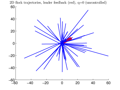
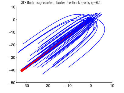
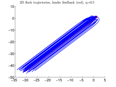
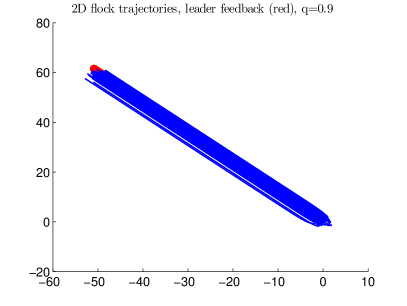
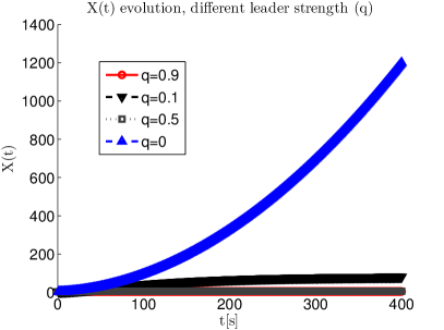
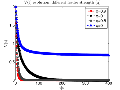
Figure 3: Leader-based feedback control. Simulations with 100 agents, the value $q$ indicates the strength of the leader in the partial average. It can be observed how, as the strength of the leader is increased, convergent behavior is improved.

Figure 4: Leader-based feedback control. Simulations with 100 agents, where $q$ indicates the strength of the leader in the partial average. Evolution of $X$ and $V$ for the simulations in Figure 4.

Besides the Cucker-Smale model, the leader-following control problem was also studied in wongkaew2015control for the Hegselmann-Krause model, and in borzi2015modeling for the D’Orsogna et al. model (see d2006self as a reference): in these papers, the leader’s optimal strategy to induce pattern formation was discussed.

4.3 Feedback under perturbed information

Motivated by the example of the last section, we turn our attention to the study of systems like (18) where the perturbation of the mean of the $i$-th agent has the specific form

$$\Delta_{i}(t)=\sum^{N}_{j=1}\omega_{ij}(t)v^{\perp}_{j}(t)\quad\text{ for every }t\geq 0,$$ (22)

for some positive measurable mapping $\omega:{\mathbb{R}}_{+}\rightarrow{\mathbb{R}}^{N\times N}$, i.e., for every $t\geq 0$ the function $\omega$ has the property $\omega_{ij}(t)>0$ for all $i,j=1,\ldots,N$.

An example of the above framework is provided by a weight matrix of the form

$$\omega_{ij}(t)\stackrel{{\scriptstyle\Delta}}{{=}}\frac{\phi(\|x_{i}(t)-x_{j}(t)\|)}{\eta_{i}(t)}\quad\text{ for every }t\geq 0.$$

where the weighting function $\phi$ corresponds to the Cucker-Smale kernel (8) with $H=1,\sigma=1$ and $\beta=\epsilon$, i.e.,

$$\phi(r)\stackrel{{\scriptstyle\Delta}}{{=}}\frac{1}{(1+r^{2})^{\epsilon}}.$$

and the normalizing terms $\eta_{i}$ are defined as

$$\eta_{i}(t)\stackrel{{\scriptstyle\Delta}}{{=}}\sum^{N}_{j=1}\phi(\|x_{i}(t)-x_{j}(t)\|).$$ (23)

Let us consider the case $\alpha(t)=\alpha>0$ and $\beta(t)=\beta>0$ for every $t\geq 0$. Figures 6 and 6 show the behavior of the system when changing the balance between the constants $\alpha$ and $\beta$. In this test, we fix a large value of $\beta=10$, representing a strong perturbation of the feedback, and a small value of $\epsilon=1e-5$, related to a disturbance which is distributed among all the agents: increasing the value of $\alpha$ in system (18) (which represents the energy of the correct information feedback) induces faster consensus emergence.

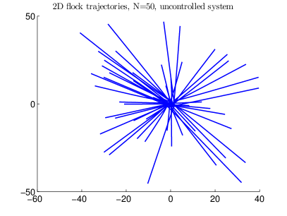
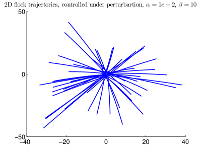
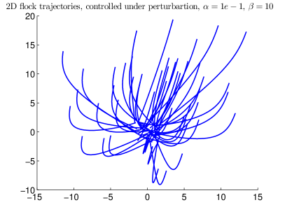
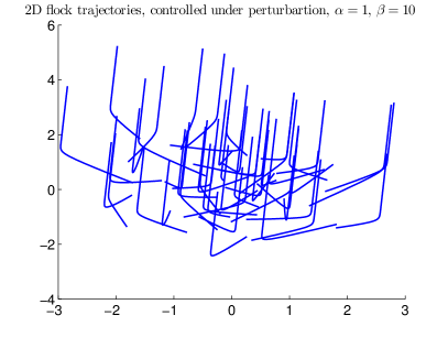
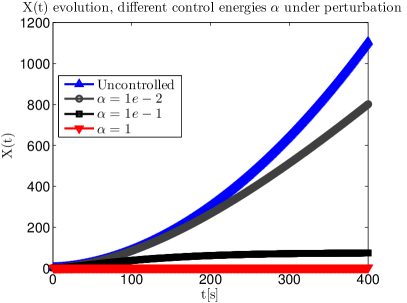
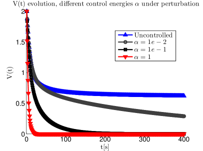
Figure 5: Total feedback control under structured perturbations. For a fixed strong structured perturbation term ($\beta=10$), different energies for the unperturbed control term $\alpha$ generate different consensus behavior; the stronger the correct information term is, the faster consensus is achieved.

Figure 6: Total feedback control under structured perturbations. Evolution of $X$ and $V$ for the simulations in Figure 6.

As already mentioned in Section 3, the use of a common normalizing factor $\eta$ in place of different terms $\eta_{i}$ greatly helps in the study of consensus emergence. For this particular case we get the following result.

Corollary 4 ((bongini2015conditional, , Corollary 3))

Suppose that for all $i,j=1,\ldots,N$ the function $\omega_{ij}:{\mathbb{R}}_{+}\rightarrow{\mathbb{R}}_{+}$ satisfies

$$\omega_{ij}(t)=\frac{\phi(\|x_{i}(t)-x_{j}(t)\|)}{\eta(t)}\quad\text{ for every }t\geq 0,$$

where $\phi:{\mathbb{R}}_{+}\rightarrow\left(0,1\right]$ is a non increasing, positive, bounded function, and $\eta:{\mathbb{R}}_{+}\rightarrow{\mathbb{R}}_{+}$ is a nonnegative bounded function satisfying

$$1\leq N\frac{\beta(t)}{\alpha(t)}\leq\eta(t)\quad\text{for every }t\geq 0.$$

Then, any solution of system (18) with $\Delta_{i}$ as in (22) tends to consensus.

Remark 7

A concrete example of a system for which we can apply Corollary 4 is obtained by considering the common normalizing term

$$\eta(t)\stackrel{{\scriptstyle\Delta}}{{=}}\max_{1\leq i\leq N}\left\{\sum^{N}_{j=1}\phi(\|x_{i}(t)-x_{j}(t)\|)\right\}.$$

which is also coherent with the asymptotic behavior of (23) for $\epsilon\rightarrow 0$ and $\epsilon\rightarrow+\infty$.

Remark 8

The request of positivity of the function $\phi$ cannot be removed from Corollary 4, see (bongini2015conditional, , Remark 4)

4.4 Perturbations due to local averaging

An interesting case of a system like (17) is the one where the local mean is given by

$$\overline{v}_{i}(t)=\frac{1}{|\Lambda_{R}(t,i)|}\sum_{j\in\Lambda_{R}(t,i)}v_{j}(t)\quad\text{ for every }t\geq 0,$$ (24)

where $\Lambda_{R}(i)$ is defined as in (5). In this case, we model the situation in which each agent estimates the average velocity of the group in the extra feedback term by only counting those agents inside a ball of radius $R$ centered on him.

Simulations in Figure 7 illustrate the behavior of such configuration. From an uncontrolled system, represented by a local feedback radius $R=0$, by increasing this quantity, partial alignment is consistently achieved, until full consensus is observed for large radii mimicking a total information feedback control.

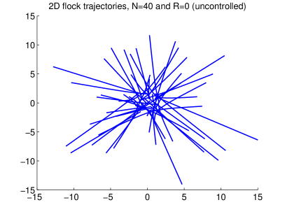
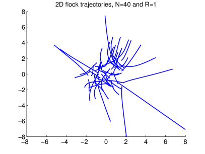
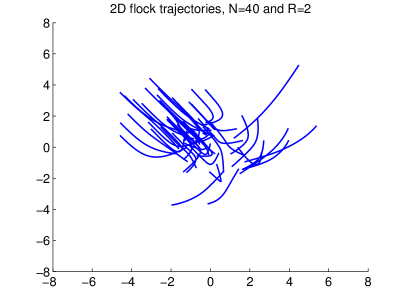
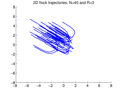
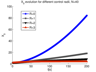
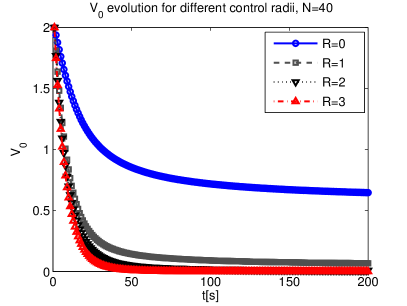
Figure 7: Local feedback control. Simulations with $N=40$ agents, and different control radii $R$. By increasing the value of $R$ the systems transits from uncontrolled behavior, to partial alignment, up to total, fast alignment.

We want to address the issue of characterizing the behavior of system (17) with the above choice for $\overline{v}_{i}$ when the radius $R$ of each ball is either reduced to $0$ or set to grow to $+\infty$. We shall see that we can reformulate this decentralized system again as a Cucker-Smale model for a different interaction function for which we can apply Theorem 3.1. We shall show how tuning the radius $R$ affects the convergence to consensus, from the case $R\geq 0$ where only conditional convergence is ensured, to the unconditional convergence result given for $R=+\infty$.

Preserving the asymptotics

First of all, by means of $\chi_{[0,R]}$ we can rewrite $\overline{v}_{i}(t)$ as

$$\overline{v}_{i}(t)=\frac{1}{\sum^{N}_{k=1}\chi_{[0,R]}(\|x_{i}(t)-x_{k}(t)\|)}\sum_{j=1}^{N}\chi_{[0,R]}(\|x_{i}(t)-x_{j}(t)\|)v_{j}(t).$$ (25)

Unfortunately, the normalizing terms $\sum^{N}_{k=1}\chi_{[0,R]}(\|x_{i}(t)-x_{k}(t)\|)$ give rise to a matrix of weights which is not symmetric, which greatly complicates the analysis of the convergence to consensus. However, since we are mainly interested in the limit behavior of the system for $R\rightarrow 0$ and $R\rightarrow+\infty$, following Remark 7 we take $\eta_{R}$ to be a function approximating the above normalizing terms and which also preserves its asymptotics for $R\rightarrow 0$ and $R\rightarrow+\infty$, as for instance,

$$\eta_{R}(t)=\max_{1\leq i\leq N}\left\{\sum^{N}_{k=1}\chi_{[0,R]}(\|x_{i}(t)-x_{k}(t)\|)\right\}.$$ (26)

Therefore, we replace the vector $\overline{v}_{i}(t)$ by

$$\frac{1}{\eta_{R}(t)}\sum^{N}_{j=1}\chi_{[0,R]}(\|x_{i}(t)-x_{j}(t)\|)v_{j}(t)\,.$$

On top of this, notice that the vector

$$\left(\frac{1}{\eta_{R}(t)}\sum^{N}_{j=1}\chi_{[0,R]}(\|x_{i}(t)-x_{j}(t)\|)\right)v_{i}(t)$$

is an approximation of $v_{i}(t)$ for $R\rightarrow 0$ and $R\rightarrow+\infty$. This motivates the replacement of the term $\overline{v}_{i}-v_{i}$ where $\overline{v}_{i}$ is as in (25) with

$$\overline{v}_{i}-v_{i}\approx\frac{1}{\eta_{R}}\sum^{N}_{j=1}\chi_{[0,R]}(\|x_{i}-x_{j}\|)v_{j}-\left(\frac{1}{\eta_{R}}\sum^{N}_{j=1}\chi_{[0,R]}(\|x_{i}-x_{j}\|)\right)v_{i}.$$ (27)

The term (27) can be rewritten as $1/\eta_{R}\sum^{N}_{j=1}\chi_{[0,R]}(\|x_{i}-x_{j}\|)(v_{j}-v_{i})$, which can be further simplified as follows

$$\begin{split}\frac{1}{\eta_{R}}\sum^{N}_{j=1}\chi_{[0,R]}(r_{ij})(v_{j}-v_{i})&=\frac{1}{\eta_{R}}\sum^{N}_{i=1}(v_{j}-v_{i})+\frac{1}{\eta_{R}}\sum^{N}_{j=1}(1-\chi_{[0,R]}(r_{ij}))(v_{i}-v_{j})\\ &=\frac{N}{\eta_{R}}\left(\overline{v}-v_{i}\right)+\frac{1}{\eta_{R}}\sum^{N}_{j=1}(1-\chi_{[0,R]}(r_{ij}))(v_{i}-v_{j}),\end{split}$$ (28)

where we have written $r_{ij}$ in place of $\|x_{i}-x_{j}\|$ and removed the time dependencies for the sake of compactness.

It is clear that the choice of the function $\chi_{[0,R]}$ is arbitrary and other alternatives can be selected, provided they give a coherent approximation of the local average (24). For instance, instead of $\chi_{[0,R]}$ and $\eta_{R}$, we can consider two generic functions $\psi_{\varepsilon}$ and $\eta_{\varepsilon}$, where $\varepsilon$ is a parameter ranging in a nonempty set $\Omega$, satisfying the following properties:

1. $\psi_{\varepsilon}:{\mathbb{R}}_{+}\rightarrow[0,1]$ is a nonincreasing measurable function for every $\varepsilon\in\Omega$;

2. $\eta_{\varepsilon}\in L^{\infty}({\mathbb{R}}_{+})$ for every $\varepsilon\in\Omega$;

3. there are two disjoint subsets $\Omega_{C\!S}$ and $\Omega_{U}$ of $\Omega$ such that

   • if $\varepsilon\in\Omega_{C\!S}$ then $\psi_{\varepsilon}=\chi_{\{0\}}$ and $\eta_{\varepsilon}\equiv 1$;

   • if $\varepsilon\in\Omega_{U}$ then $\psi_{\varepsilon}=\chi_{{\mathbb{R}}_{+}}$ and $\eta_{\varepsilon}\equiv N$.

Under the above hypotheses, we consider the perturbation given for every $t\geq 0$ by

$$\Delta^{\varepsilon}_{i}(t)\stackrel{{\scriptstyle\Delta}}{{=}}\frac{1}{\eta_{\varepsilon}(t)}\sum^{N}_{j=1}(1-\psi_{\varepsilon}(\|x_{i}(t)-x_{j}(t)\|))(v_{i}(t)-v_{j}(t)).$$ (29)

With requirement $(iii)$ we impose that whenever $\varepsilon\in\Omega_{C\!S}$ then it holds

$$\Delta_{i}^{\varepsilon}(t)=-\frac{N}{\eta_{\varepsilon}(t)}(\overline{v}(t)-v_{i}(t)),$$

therefore recovering the Cucker-Smale system (7) from (30), while whenever $\varepsilon\in\Omega_{U}$ then $\Delta_{i}^{\varepsilon}(t)=0$ holds, and we obtain a particular instance of system (16).

The enlarged consensus region

By means of (28) and (29), we can rewrite our system with the local average (24) in the form of system (18) as follows

$$\left\{\begin{aligned} \hfil\displaystyle\begin{split}\dot{x}_{i}(t)&=v_{i}(t),\\ \dot{v}_{i}(t)&=\frac{1}{N}\sum_{j=1}^{N}a\left(\|x_{i}(t)-x_{j}(t)\|\right)\left(v_{j}(t)-v_{i}(t)\right)+\gamma\frac{N}{\eta_{\varepsilon}(t)}(\overline{v}(t)-v_{i}(t))+\gamma\Delta^{\varepsilon}_{i}(t).\end{split}\end{aligned}\right.$$ (30)

Using (28) and collecting the term $(v_{j}-v_{i})$, it is easy to see that Theorem 3.1 yields the following description of the consensus region as a function of the parameter $\varepsilon$.

Theorem 4.2

Fix $\gamma\geq 0$, consider system (30) where $\Delta^{\varepsilon}_{i}$ is as in (29) and let $(x^{0},v^{0})\in{\mathbb{R}}^{dN}\times{\mathbb{R}}^{dN}$. If $X_{0}\stackrel{{\scriptstyle\Delta}}{{=}}B(x^{0},x^{0})$ and $V_{0}\stackrel{{\scriptstyle\Delta}}{{=}}B(v^{0},v^{0})$ satisfy

$$\int^{+\infty}_{\sqrt{X_{0}}}a\left(\sqrt{2N}r\right)\ dr+\frac{\gamma N}{\left\|{\eta_{\varepsilon}}\right\|_{L^{\infty}({\mathbb{R}}_{+})}}\int^{+\infty}_{\sqrt{X_{0}}}\psi_{\varepsilon}\left(\sqrt{2N}r\right)\ dr\geq\sqrt{V_{0}},$$ (31)

then the solution of system (30) with initial datum $(x^{0},v^{0})$ tends to consensus.

Let us see how we can apply Theorem 4.2 to obtain an estimate of the consensus region for the local average (24). We consider $\Omega=[0,+\infty]$, the sequence of functions $(\chi_{[0,R]})_{R\in\Omega}$ and $\eta_{R}$ as in (26) (notice that, as before, we have $\Omega_{C\!S}=\{0\}$ and $\Omega_{U}=\{\infty\}$). Since it holds $\left\|{\eta_{R}}\right\|_{L^{\infty}({\mathbb{R}}_{+})}\leq N$, if $R$ is sufficiently large to satisfy $\sqrt{2NX_{0}}\leq R$, condition (31) is satisfied as soon as

$$\int^{+\infty}_{\sqrt{X_{0}}}a\left(\sqrt{2N}r\right)\ dr+\gamma\left(\frac{R}{\sqrt{2N}}-\sqrt{X_{0}}\right)\geq\sqrt{V_{0}},$$

by means of a trivial integration. If, instead, $R$ is so small that $\sqrt{2NX_{0}}>R$ holds, condition (31) is satisfied as soon as

$$\int^{+\infty}_{\sqrt{X_{0}}}a\left(\sqrt{2N}r\right)\ dr\geq\sqrt{V_{0}},$$

recovering Theorem 3.1. As can be seen, we have enlarged the original consensus region provided by Theorem 3.1 by a term whose size is linearly increasing in $R$. This implies that, in the case $R=+\infty$, the consensus region coincides with the entire space ${\mathbb{R}}^{dN}\times{\mathbb{R}}^{dN}$, hence the system converges to consensus regardless of the initial datum.

Empirical estimation of the enlarged consensus region

We present a series of numerical tests aiming at estimating empirically the enlarged consensus region given by (31) following similar ideas as those presented in cafotove10 . We consider a system of $N$ agents in dimension $d=2$ with a randomly generated initial configuration of positions and velocities

$$(x^{0},v^{0})\in[-1,1]^{2N}\times[-1,1]^{2N}\,,$$

interacting by means of the kernel (8) with $H=1$, $\sigma=1$ and $\beta=1$. We recall that relevant quantities for the analysis of our results are given by (here we stress the dependance on $x$ and $v$)

$$X[x](t)\stackrel{{\scriptstyle\Delta}}{{=}}\frac{1}{2N^{2}}\sum_{i,j=1}^{N}\|x_{i}(t)-x_{j}(t)\|^{2}\quad\text{and}\quad V[v](t)\stackrel{{\scriptstyle\Delta}}{{=}}\frac{1}{2N^{2}}\sum_{i,j=1}^{N}\|v_{i}(t)-v_{j}(t)\|^{2}\,.$$

Notice that, once a random initial configuration has been generated, it is possible to rescale it to a desired $(X_{0},V_{0})$ parametric pair, by means of

$$(x,v)=\left(\sqrt{\frac{X_{0}}{X[\tilde{x}]}}\tilde{x},\sqrt{\frac{V_{0}}{V[\tilde{v}]}}\tilde{v}\right)\,,$$

such that $(X[x],V[v])=(X_{0},V_{0})$. As simulations of the trajectories have been generated by prescribing a value for the pair $(X_{0},V_{0})$, which is used to rescale randomly generated initial conditions, there are slight variations on the initial positions and velocities in every model run, which can affect the final consensus direction. However our results are stated in terms of $X,V$, and independently of the specific initial configuration. For simulation purposes the system is integrated in time with the specific feedback control by means of a Runge-Kutta 4th-order scheme.

As it was shown in Example 1, that estimates for consensus regions such as the one provided by Theorem 3.1, are not sharp in many situations. In this direction, we proceed to contrast the theoretical consensus estimates with the numerical evidence. For this purpose, for a fixed number of agents, we span a large set of possible initial configurations determined by different values of $(X_{0},V_{0})$. For every pair $(X_{0},V_{0})$ we randomly generate a set of 20 initial conditions, and we simulate for a sufficiently large time frame. We measure consensus according to a threshold established on the final value of $V$; we consider that consensus has been achieved if the final value of $V$ is lower or equal to $1e-5$. We proceed by computing empirical probabilities of consensus for every point of our state space $(X_{0},V_{0})$; results in this direction are presented in Figures 8 and 9. We first consider the simplified case of 2 agents; according to Example 1, for this particular case, the consensus region estimate provided by Theorem 3.1 is sharp, as illustrated by the results presented in Figure 8. Furthermore, it is also the case for Theorem 4.2; for $R>0$, the predicted consensus region coincides with the numerically observed ones.

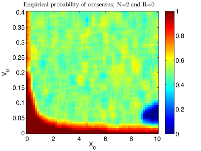
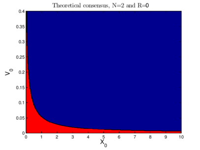
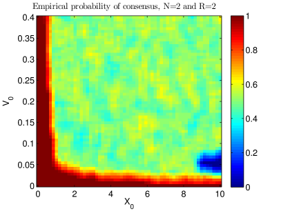
Figure 8: Local feedback control. Empirical consensus regions and theoretical estimates for two-agent systems.

Figure 9 illustrates the case when a larger number of agents is considered. In a similar way as for Theorem 3.1, the consensus region estimate is conservative if compared with the region where numerical experiments exhibit convergent behavior. Nevertheless, Theorem 4.2 is consistent in the sense that the theoretical consensus region increases gradually as $R$ grows, eventually covering any initial configuration, which is the case of the total information feedback control, as presented in (caponigro2015sparse, , Proposition 2). The numerical experiments also confirm this phenomena, as shown in Figure 10, where contour lines showing the $80\%$ probability of consensus for different radii locate farther from the origin as $R$ increases.

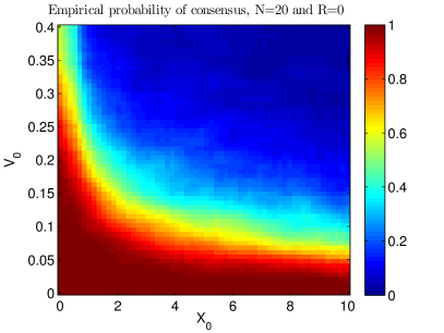
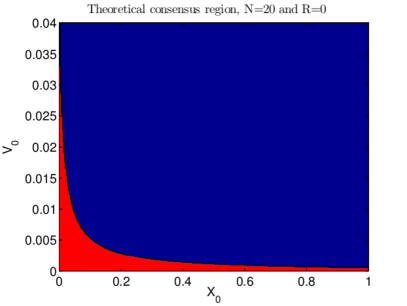
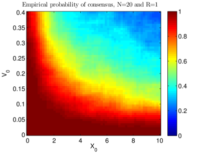
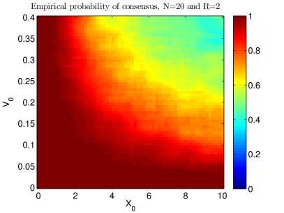
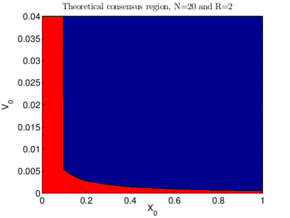
Figure 9: Local feedback control. Empirical consensus regions and theoretical estimates for $N=20$ agents and different control radii $R$.

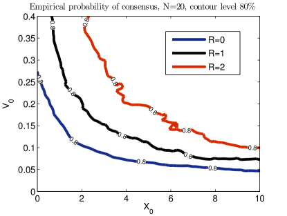
Figure 10: Local feedback control. Empirical contour lines for the 80$\%$ probability of consensus with different control radii.

5 Sparse control of the Cucker-Smale model

We have seen throughout the previous sections how difficult it is to ensure unconditional convergence to consensus for alignment models. In particular, in Section 4.4 we have proven that the addition of a local feedback does not always help: Theorem 4.2 shows that we can guarantee unconditional convergence to consensus with respect to the initial datum for dynamical systems of the form

$$\left\{\begin{aligned} \hfil\displaystyle\begin{split}\dot{x}_{i}(t)&=v_{i}(t),\\ \dot{v}_{i}(t)&=\frac{1}{N}\sum_{j=1}^{N}a\left(\left\|{x_{i}(t)-x_{j}(t)}\right\|\right)\left(v_{j}(t)-v_{i}(t)\right)+\gamma\left(\frac{1}{|\Lambda_{R}(t,i)|}\sum_{j\in\Lambda_{R}(t,i)}v_{j}(t)-v_{i}(t)\right).\end{split}\end{aligned}\right.$$

only in the case $R=+\infty$, for which the identity

$$\frac{1}{|\Lambda_{R}(t,i)|}\sum_{j\in\Lambda_{R}(t,i)}v_{j}(t)=\overline{v}(t)$$

holds. This means that either the agents have perfect information of the state of the entire system (so that the local mean $\overline{v}_{i}$ is equal to the true mean $\overline{v}$) or, as the numerical simulations in Section 4.4 show, there are situations where the agents are not able to converge to consensus. As already pointed out in Section 4, this is a very strong requirement to ask for, and not many real-life scenarios are able to support it. Consider, for instance, the case of an assembly of people trying to reach an unanimous decision, like the European Union Council: since the extra term can be interpreted as an additional desire of each agent to agree with people whose goal is near to his, the requirement $R=+\infty$ corresponds to asking that all the individual goals are close, i.e., all agents pursue the same end. A truly imaginative world indeed! We are thus facing an inherent, severe limitation of the decentralized approach.

5.1 Centralized feedback interventions

To overcome this apparent dead-end, let us write $u_{i}(t)=\gamma(\overline{v}(t)-v_{i}(t))$, i.e.,

$$\left\{\begin{aligned} \hfil\displaystyle\begin{split}\dot{x}_{i}(t)&=v_{i}(t),\\ \dot{v}_{i}(t)&=\frac{1}{N}\sum_{j=1}^{N}a\left(\left\|{x_{i}(t)-x_{j}(t)}\right\|\right)\left(v_{j}(t)-v_{i}(t)\right)+u_{i}(t).\end{split}\end{aligned}\right.$$ (32)

Instead of interpreting $u_{i}$ as a decentralized force, let us consider it as an external force from an outside source acting on the system to help it to coordinate. This new approach sheds a completely different light on the problem: with respect to the example considered before, is like introducing a moderator heading the discussion, who can make pressure on the participants to the council facilitating the consensus process. Adding an external figure implementing intervention policies broadens further the expressive power of the problem: indeed, since we are in principle no more tied to specific interventions of the form $u_{i}(t)=\gamma(\overline{v}(t)-v_{i}(t))$, this setting enables us to ask ourselves the following question

(Q) given a set of constraints, which control $u$ is the best to reach a specific goal?

In this section, we shall study a specific instance of this very general issue in the case of system (32). In our setting, the constraints shall be

1. the control is of feedback-type, i.e., computed instantaneously as a function of the state variables, following a locally optimal criterion;

2. there is a maximal amount of resources $M>0$ that the central policy maker can spend at any given time for the intervention;

3. the control should act on the least amount of agents possible at any time.

For the time being, our goal is again alignment, hence we seek for a control $u$ for which the associated solution to system (32) tends to consensus in the sense of Definition 3. We have seen in Proposition 1 that an effective criterion for consensus emergence is the minimization of the Lyapunov functional $V$: if we are able to prove that our control strategy is able to drive $V$ below the threshold level given by Theorem 3.1, we have automatically consensus emergence (see Figure 11). The maximization of the decay rate of $V$ is a locally optimal criterion, and hence compatible with point ($i$).

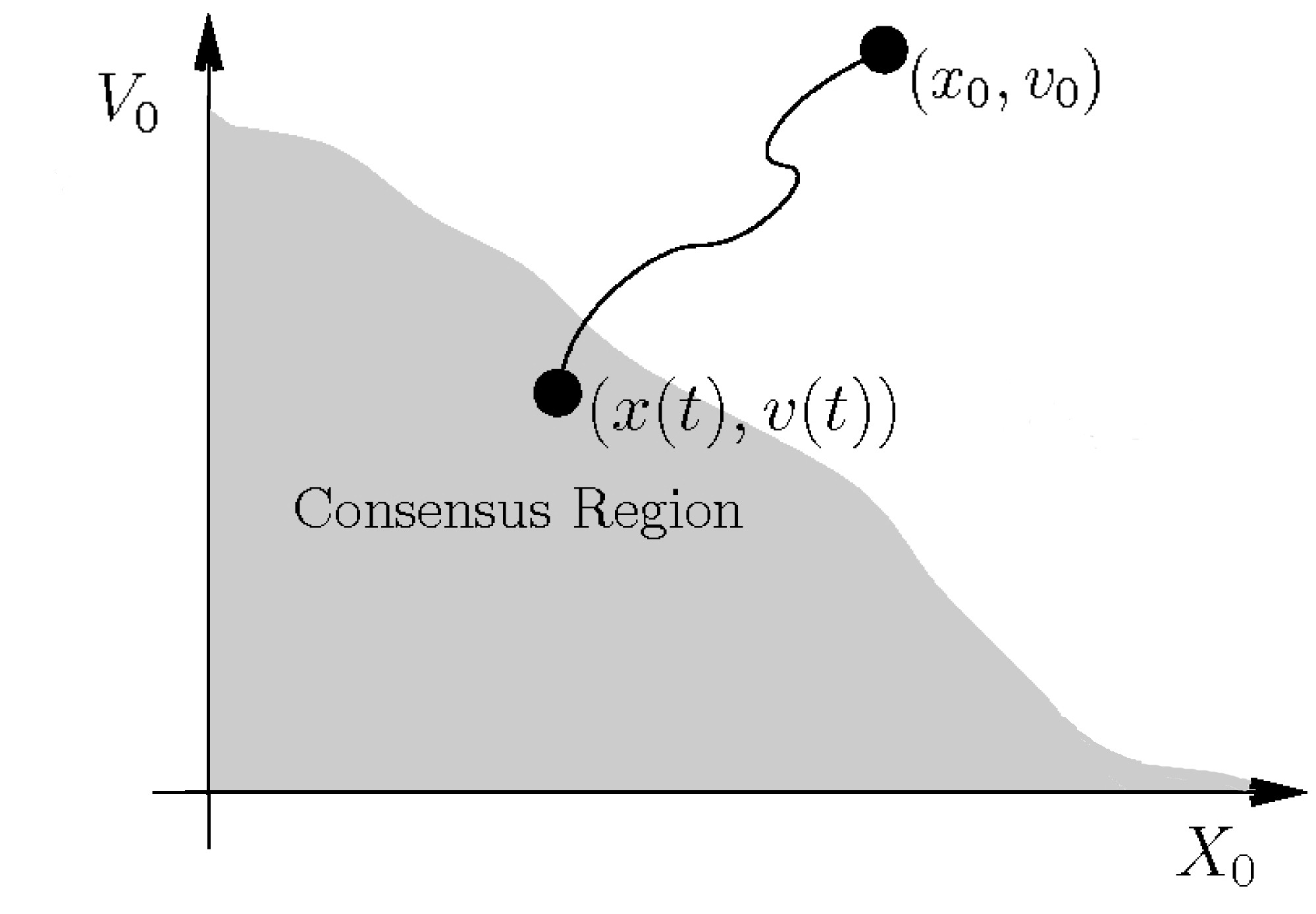
Figure 11: Steering the system to a point fulfilling the conditions of Theorem 3.1.

The following preliminary estimate shows the effect of a control on $V$.

Lemma 3

For any measurable function $u:{\mathbb{R}}_{+}\rightarrow{\mathbb{R}}^{dN}$ it holds

$$\frac{d}{dt}V(t)\leq 2B(u(t),v(t)).$$

Proof

Using the representation of system (7) in Laplacian form (9), and the fact that $L(x(t))$ is positive definite, we get

$$\frac{d}{dt}V(t)=\frac{d}{dt}B(v(t),v(t))=-2B(L(x(t))v(t),v(t))+2B(u(t),v(t))\leq 2B(u(t),v(t)).$$

This concludes the proof.

The constraint on the maximal amount of available resources $M$ given by point ($ii$) leads to the following definition of admissible controls.

Definition 6 (Admissible controls)

A measurable function $u=(u_{1},\ldots,u_{N}):{\mathbb{R}}_{+}\rightarrow{\mathbb{R}}^{dN}$ is an admissible control if it satisfies

$$\sum^{N}_{i=1}\|u_{i}(t)\|\leq M\quad\text{ for every }t\geq 0.$$ (33)

As an immediate corollary of Lemma 3 we can show that the problem of finding admissible controls steering the system to consensus is well-posed.

Corollary 5 (Total control, (caponigro2015sparse, , Proposition 2))

Fix $M>0$, an initial condition $(x^{0},v^{0})\in{\mathbb{R}}^{dN}\times{\mathbb{R}}^{dN}$, and $0<\alpha\leq M/(N\sqrt{V_{0}})$. Then, the feedback control defined pointwise in time as

$$u(t)=-\alpha v^{\perp}(t)\quad\text{ for every }t\geq 0,$$ (34)

is admissible and the solution associated to $u$ tends to consensus.

Proof

Let $(x,v):{\mathbb{R}}_{+}\rightarrow{\mathbb{R}}^{dN}\times{\mathbb{R}}^{dN}$ be a solution of system (32) with $u$ as in the statement. Lemma 3 implies that

$$\frac{d}{dt}V(t)\leq 2B(u(t),v(t))=-2\alpha B(v^{\perp}(t),v(t))=-2\alpha V(t);$$

Therefore, an application of Gronwall’s Lemma yields $V(t)\leq e^{-2\alpha t}V(0)$, so $V(t)$ tends to $0$ exponentially fast as $t\rightarrow+\infty$. In particular, $X(t)$ keeps bounded and the trajectory reaches the consensus region in finite time. Lastly, it follows that

$$\sum^{N}_{i=1}\|u_{i}(t)\|\leq\sqrt{N}\sqrt{\sum^{N}_{i=1}\|u_{i}(t)\|^{2}}=\alpha\sqrt{N}\sqrt{\sum^{N}_{i=1}\|v^{\perp}_{i}(t)\|^{2}}=\alpha N\sqrt{V(t)}\leq\alpha N\sqrt{V_{0}}\leq M,$$

which implies the admissibility of the control.

Corollary 5, although very simple, is somehow remarkable: not only it shows that we can steer to consensus the system from any initial condition, but that the strength of the control $M>0$ can be arbitrarily small. However, this result has perhaps only theoretical validity, because the stabilizing control $u=-\alpha v^{\perp}$ needs to act instantaneously on all the agents, thus requires the external policy maker to interact at every instant with all the agents in order to steer the system to consensus, a procedure that requires a large amount of instantaneous communications, whence the name of total control. This motivates point ($iii$) and is the reason why we look for interventions that target the fewest number of agents at any given time. However, this leads us into the difficult combinatorial problem of the selection of the best few control components to be activated. How can we solve it?

The problem resembles very much the one in information theory of finding the best possible sparse representation of data in form of vector coefficients with respect to an adapted dictionary for the sake of their compression, see (mallat2008wavelet, , Chapter 1). In our case, the relationship between control choices and result will be usually highly nonlinear, especially for several known dynamical systems modeling social dynamics: were this relationship more simply linear instead, then a rather well-established theory would predict how many degrees of freedom are minimally necessary to achieve the expected outcome. Moreover, depending on certain spectral properties of the linear model, the theory allows also for efficient algorithms to compute the relevant degrees of freedom, relaxing the associated combinatorial problem. This theory is known in mathematical signal processing and information theory under the name of compressed sensing, see the seminal work tao ; donoho and the review chapter fora10 . The major contribution of these papers was to realize that one can combine the power of convex optimization, in particular $\ell_{1}$-norm minimization, and spectral properties of random linear models in order to achieve optimal results on the ability of $\ell_{1}$-norm minimization of recovering robustly linearly constrained sparsest solutions. Borrowing a leaf from compressed sensing, we model sparse stabilization and control strategies by penalizing the class of vector-valued controls $u=(u_{1},\ldots,u_{N})\in{\mathbb{R}}^{dN}$ by means of the mixed $\ell^{N}_{1}-\ell^{d}_{2}$-norm

$$\sum^{N}_{i=1}\|u_{i}\|_{\ell^{d}_{2}}$$

The above mixed norm has been already used, for instance, in elra10 to optimally sparsify multivariate vectors in compressed sensing problems, or in fora08 as a joint sparsity constraint. The use of $\ell_{1}$-norms to penalize controls was first introduced in the seminal paper crlo65 to model linear fuel consumption, while lately the use of $L^{1}$ minimization in optimal control problems with partial differential equation has become very popular, for instance in the modeling of optimal placing of sensors caclku12 ; clku12 ; hestwa12 ; st09 ; wawa11 .

5.2 Sparse feedback controls

We wonder whether we can stabilize the system by means of interventions that are more parsimonious than the total control, since they are more realistically modeling actual government actions. From Lemma 3, we learn that a good strategy to steer the system to consensus is actually the minimization of $B(u(t),v(t))$ with respect to $u$, for all $t$. For this reason, we choose controls according to a specific variational principle leading to a componentwise sparse stabilizing feedback law.

Definition 7

For every $M>0$ and every $(x,v)\in{\mathbb{R}}^{dN}\times{\mathbb{R}}^{dN}$, let $U(x,v)$ be the set of solutions of the variational problem

$$\min_{u\in{\mathbb{R}}^{dN}}\left(B(u,v)+\gamma(B(x,x))\frac{1}{N}\sum^{N}_{i=1}\|u_{i}\|\right)\quad\text{ subject to }\sum^{N}_{i=1}\|u_{i}\|\leq M,$$ (35)

where the threshold functional $\gamma$ is defined as

$$\gamma(X)\stackrel{{\scriptstyle\Delta}}{{=}}\int^{\infty}_{\sqrt{X}}a(\sqrt{2N}r)dr.$$

Notice that the variational principle (35) is balancing the minimization of $B(u,v)$, which we mentioned above as relevant to promote convergence to consensus, and the $\ell_{1}$-norm term $\sum^{N}_{i=1}\|u_{i}\|$, expected to promote sparsity.

Each value of $\gamma(B(x,x))$ yields a partition of ${\mathbb{R}}^{dN}\times{\mathbb{R}}^{dN}$ into four disjoint sets:

$\mathcal{P}_{1}$

$\stackrel{{\scriptstyle\Delta}}{{=}}\{(x,v)\in{\mathbb{R}}^{dN}\times{\mathbb{R}}^{dN}:\max_{1\leq i\leq N}\left\|{v^{\perp}_{i}}\right\|<\gamma(B(x,x))^{2}\}$,

$\mathcal{P}_{2}$

$\stackrel{{\scriptstyle\Delta}}{{=}}\{(x,v)\in{\mathbb{R}}^{dN}\times{\mathbb{R}}^{dN}:\max_{1\leq i\leq N}\left\|{v^{\perp}_{i}}\right\|=\gamma(B(x,x))^{2}\text{ and }\exists k\geq 1\text{ and }i_{1},\ldots,i_{k}\break\in\{1,\ldots N\}$ $\text{ such that }\left\|{v^{\perp}_{i_{1}}}\right\|=\ldots=\left\|{v^{\perp}_{i_{k}}}\right\|\text{ and }\left\|{v^{\perp}_{i_{1}}}\right\|>\left\|{v^{\perp}_{j}}\right\|\text{ for every }j\not\in\{i_{1},\ldots,i_{k}\}\}$,

$\mathcal{P}_{3}$

$\stackrel{{\scriptstyle\Delta}}{{=}}\{(x,v)\in{\mathbb{R}}^{dN}\times{\mathbb{R}}^{dN}:\max_{1\leq i\leq N}\left\|{v^{\perp}_{i}}\right\|>\gamma(B(x,x))^{2}\text{ and }\exists!i\in\{1,\ldots N\}\text{ such}\\ \text{ that }\left\|{v^{\perp}_{i}}\right\|>\left\|{v^{\perp}_{j}}\right\|\text{ for every }j\not=i\}$,

$\mathcal{P}_{4}$

$\stackrel{{\scriptstyle\Delta}}{{=}}\{(x,v)\in{\mathbb{R}}^{dN}\times{\mathbb{R}}^{dN}:\max_{1\leq i\leq N}\left\|{v^{\perp}_{i}}\right\|>\gamma(B(x,x))^{2}\text{ and }\exists k>1\text{ and }i_{1},\ldots,i_{k}\break\in\{1,\ldots N\}$ $\text{ such that }\left\|{v^{\perp}_{i_{1}}}\right\|=\ldots=\left\|{v^{\perp}_{i_{k}}}\right\|\text{ and }\left\|{v^{\perp}_{i_{1}}}\right\|>\left\|{v^{\perp}_{j}}\right\|\text{ for every }j\not\in\{i_{1},\ldots,i_{k}\}\}$,

Moreover, since we are minimizing $B(u,v)=B(u,v^{\perp})$, it is easy to see that, for every $(x,v)\in{\mathbb{R}}^{dN}\times{\mathbb{R}}^{dN}$ and every element $u(x,v)=(u_{1}(x,v),\dots,u_{N}(x,v))^{T}\in U(x,v)$ there exist nonnegative real numbers $\varepsilon_{i}\geq 0$ such that, for every $i=1,\ldots,N$, it holds

$$u_{i}(x,v)=\begin{cases}\displaystyle-\varepsilon_{i}\frac{v^{\perp}_{i}}{\|v^{\perp}_{i}\|}&\quad\text{ if }\|v^{\perp}_{i}\|\not=0,\\ 0&\quad\text{ if }\|v^{\perp}_{i}\|=0,\end{cases}$$ (36)

where $0\leq\sum^{N}_{i=1}\varepsilon_{i}\leq M$. The values of the $\varepsilon_{i}$’s can be determined on the basis of which partition $(x,v)$ belongs to:

• if $(x,v)\in\mathcal{P}_{1}$ then $\varepsilon_{i}=0$ for every $i=1,\ldots,N$;

• if $(x,v)\in\mathcal{P}_{2}$ then indicating with $i_{1},\ldots,i_{k}$ the indexes such that $\left\|{v^{\perp}_{i_{1}}}\right\|=\ldots=\left\|{v^{\perp}_{i_{k}}}\right\|=\gamma(B(x,x))$ and $\left\|{v^{\perp}_{i_{1}}}\right\|>\left\|{v^{\perp}_{j}}\right\|$ for every $j\not\in\{i_{1},\ldots,i_{k}\}$, we have $\varepsilon_{j}=0$ for every $j\not\in\{i_{1},\ldots,i_{k}\}$;

• if $(x,v)\in\mathcal{P}_{3}$ then, indicating with $i$ the only index such that $\left\|{v^{\perp}_{i}}\right\|>\left\|{v^{\perp}_{j}}\right\|$ for every $j\not=i$, we have $\varepsilon_{i}=M$ and $\varepsilon_{j}=0$ for every $j\not=i$;

• if $(x,v)\in\mathcal{P}_{4}$ then, indicating with $i_{1},\ldots,i_{k}$ the indexes such that $\left\|{v^{\perp}_{i_{1}}}\right\|=\ldots=\left\|{v^{\perp}_{i_{k}}}\right\|$ and $\left\|{v^{\perp}_{i_{1}}}\right\|>\left\|{v^{\perp}_{j}}\right\|$ for every $j\not\in\{i_{1},\ldots,i_{k}\}$, we have $\varepsilon_{j}=0$ for every $j\not\in\{i_{1},\ldots,i_{k}\}$ and $\sum^{k}_{\ell=1}\varepsilon_{i_{\ell}}=M$.

Notice that any control $u(x,v)\in U(x,v)$ acts as an additional force which pulls agents towards having the same mean consensus parameter. The imposition of the $\ell^{N}_{1}-\ell^{d}_{2}$-norm constraint has the function of enforcing sparsity: from the observation above clearly follows that

$$U|_{\mathcal{P}_{1}}=\{0\}\quad\text{and}\quad U|_{\mathcal{P}_{3}}=\{(0,\ldots,0,-Mv^{\perp}_{i}/\|v^{\perp}_{i}\|,0,\ldots,0)^{T}\},$$

for some unique $i\in\{1,\ldots,N\}$, i.e., the restrictions of $U$ to $\mathcal{P}_{1}$ and to $\mathcal{P}_{3}$ are single-valued. However, even if not all controls belonging to $U$ are sparse, there exist selections with maximal sparsity.

Definition 8 ((caponigro2015sparse, , Definition 4))

We select the sparse feedback control $u(x,v)\in U(x,v)$ according to the following criterion:

• if $\max_{1\leq i\leq N}\left\|{v^{\perp}_{i}}\right\|\leq\gamma(B(x,x))^{2}$, then $u(x,v)=0$;

• if $\max_{1\leq i\leq N}\left\|{v^{\perp}_{i}}\right\|>\gamma(B(x,x))^{2}$, denote with $\hat{\iota}(x,v)\in\{1,\ldots,N\}$ the smallest index such that

  $$\left\|{v^{\perp}_{\hat{\iota}(x,v)}}\right\|=\max_{1\leq i\leq N}\left\|{v^{\perp}_{i}}\right\|.$$

  Then

  $$u_{j}(x,v)\stackrel{{\scriptstyle\Delta}}{{=}}\begin{cases}\displaystyle-M\frac{v^{\perp}_{\hat{\iota}(x,v)}}{\|v^{\perp}_{\hat{\iota}(x,v)}\|}&\quad\text{ if }j=\hat{\iota}(x,v),\\ 0&\quad\text{ otherwise.}\end{cases}$$

The geometrical interpretation of why the sparse feedback control is a solution of (35) is given by the graphics in Figure 12 below, representing the scalar situation.

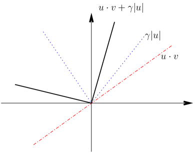
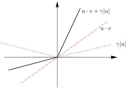
Figure 12: Geometrical interpretation of the solution of (35) in the scalar case. On the left: for $|v|\leq\gamma$ the minimal solution $u\in[-M,M]$ is zero. On the right: for $|v|>\gamma$ the minimal solution $u\in[-M,M]$ is for $|u|=M$.

The following result shows that the above feedback control strategy is capable of steering the system to the consensus region in finite time.

Theorem 5.1 ((caponigro2015sparse, , Theorem 3))

For every initial condition $(x_{0},v_{0})\in{\mathbb{R}}^{dN}\times{\mathbb{R}}^{dN}$ and $M>0$, there exist $T>0$ and a piecewise constant selection of the sparse feedback selection of Definition 8 such that the associated absolutely continuous solution reaches the consensus region at the time $T$.

This result is truly remarkable, since it holds again independently of the initial conditions and of the strength $M>0$ of the control. Furthermore, the sparse feedback control is optimal for consensus problems with respect to any other control strategy in $U(x(t),v(t))$ which spreads control over multiple agents, as the following result shows.

Proposition 3 ((caponigro2015sparse, , Proposition 3))

The sparse feedback control of Definition 8 is for every $t\geq 0$ an instantaneous minimizer of

$$\mathcal{D}(t,u)\stackrel{{\scriptstyle\Delta}}{{=}}\frac{d}{dt}V(t)$$

over all possible feedback controls in $U(x(t),v(t))$.

A direct consequence of Proposition 3 is that, for Cucker-Smale systems, a feedback stabilization is most effective if all the attention of the controller is focused on the agent farthest away from consensus. This also means that, despite the fact that the external policy maker may have few resources at disposal and can allocate them at each time only on very few key players in the system, it is always possible to effectively stabilize the dynamics to return to energy levels where the system tends autonomously to consensus. This result is perhaps surprising if confronted with the more intuitive strategy of controlling more, or even all, agents at the same time. This let us answer to the question (Q) raised at the beginning of this section as follows:

(A) under the constraints $(i)-(iii)$, sparse is better.

5.3 Numerical implementation of the sparse control strategy

We now compare the performances of the sparse feedback control with the self-organizing power of an uncontrolled Cucker-Smale system and the efficacy of the total control strategy (34). In Figure 13–left it is shown a simulation of a Cucker-Smale system with $\beta=1$ without control (in black), with the total control (in blue), and with the sparse feedback control (in red). While the uncontrolled scenario seems far from converging towards a consensus state, both the total control and the sparse control strategies successfully align the agents in very short time. The greater effectiveness of the sparse feedback control can be witnessed in Figure 13–right, where it is shown the decay of the Lyapunov functional $V$ in the three different cases: the sparse control is more efficient in bringing $V$ to $0$, as Proposition 3 predicts.

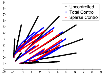
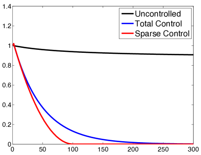
Figure 13: Comparison between sparse, total and no control. On the left: space evolution without control (in black), with the total control (in blue), and with the sparse control strategy (in red). On the right: the respective behavior of the functional $V$.

The situation where the sparse control strategy works at its bests is when the velocities of the agents are almost homogeneous, except for few outliers which are very distant from the mean velocity. As extensively discussed in bonginijunge2014sparse , in such situations the total control is suboptimal because it also acts on agents which do not need any intervention, while the sparse control strategy is locally optimal because it focuses all its strength on the small group of outliers. Such scenario is portrayed in Figure 14: starting from the same initial datum of Figure 13, we modify the velocity of one agent so that it decisively deviates from the mean velocity. This time, the difference in the outcome of the two control strategies is much more visible. More generally, an empirical detector of configurations where it is convenient to use the sparse feedback control is the so-called asymmetry measure, proposed in (bonginithesis, , Section 3.6.5).

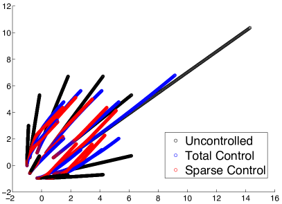
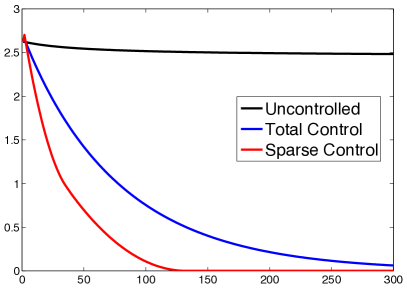
Figure 14: Configuration with one outlier. On the left: space evolution without control (in black), with the total control (in blue), and with the sparse control strategy (in red). On the right: the respective behavior of the functional $V$.

6 The Cucker-Dong model

We now show how the sparse feedback control strategy previously introduced has far more reaching potential, as it can address also situations which do not match the structure (9), like the Cucker and Dong model of cohesion and avoidance introduced in cucker14 , which is given by the following system of differential equations

$$\left\{\begin{aligned} \hfil\displaystyle\begin{split}\dot{x}_{i}(t)&=v_{i}(t),\\ \dot{v}_{i}(t)&=-b_{i}(t)v_{i}(t)+\sum_{j=1}^{N}a\left(\left\|{x_{i}(t)-x_{j}(t)}\right\|^{2}\right)\left(x_{j}(t)-x_{i}(t)\right)+\\ &\quad+\sum_{j\not=i}^{N}f\left(\left\|{x_{i}(t)-x_{j}(t)}\right\|^{2}\right)\left(x_{i}(t)-x_{j}(t)\right),\end{split}\quad i=1,\ldots,N,\end{aligned}\right.$$ (37)

The evolution is governed by an attraction force, modeled by a function $a:\mathbb{R}_{+}\rightarrow{\mathbb{R}}_{+}$, which is, for some fixed constant $H>0$ and $\beta\geq 0$, of the form

$$a(r)=\frac{H}{(1+r)^{\beta}},$$

(notice that here we have $r$ in place of $r^{2}$, since we write $a(\left\|{x_{i}-x_{j}}\right\|^{2})$ in place of $a\left(\left\|{x_{i}-x_{j}}\right\|\right)$, hence $a$ has the same form as (8)), though in general any Lipschitz-continuous, nonincreasing function with maximum in $a(0)$ suffices. This force is counteracted by a repulsion given by a locally Lipschitz continuous or $\mathcal{C}^{1}$, nonincreasing function $f:(0,+\infty)\rightarrow{\mathbb{R}}_{+}$. We request that

$$\int^{+\infty}_{\delta}f(r)\ dr<+\infty,\quad\text{ for every }\delta>0.$$

A typical example of such a function is $f(r)=r^{-p}$ for every $p>1$. The uniformly continuous, bounded functions $b_{i}:{\mathbb{R}}_{+}\rightarrow[0,\Lambda]$, $i=1,\dots,N$, for a given $\Lambda\geq 0$, are interpreted as a friction which helps the system to stay confined.

It is easily seen how the above model can be rewritten as

$$\left\{\begin{aligned} \dot{x}(t)&=v(t),\\ \dot{v}(t)&=-L(x(t))x(t)-v(t)b(t),\end{aligned}\right.$$

where for any $x\in{\mathbb{R}}^{dN}$ the function $L(x)\stackrel{{\scriptstyle\Delta}}{{=}}L^{a}(x)-L^{f}(x)$ is the difference between the Laplacians of the two matrices $(a(\left\|{x_{i}-x_{j}}\right\|^{2}))_{i,j=1}^{N}$ and $(f(\left\|{x_{i}-x_{j}}\right\|^{2}))_{i,j=1}^{N}$, respectively, and we have set $vb\stackrel{{\scriptstyle\Delta}}{{=}}(v_{i}b_{i})_{i=1}^{N}$ for any $b=(b_{1},\ldots,b_{N})$. Notice that, differently from (9), now the Laplacians are acting on the variable $x$ and not anymore on $v$, mixing the dynamics of the two components of the state: as a consequence, the Cucker-Dong model is a non-dissipative system with singular repulsive interaction forces. Similar models considering attraction, repulsion and other effects, such as alignment or self-drive, appear in the recent literature and they seem effectively describing realistic situations of conditional pattern formation, see, e.g., some of the most related contributions MR2507454 ; ChuDorMarBerCha07 ; CuckerDong11 ; d2006self .

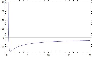
Figure 15: Sum of the attraction and repulsion forces $h(r)=f(r)-a(r)$ as a function of the distance $r>0$. The parameters here are $H=50$, $\beta=0.7$, and $p=4$.

At first glance it may seem perhaps a bit cumbersome to consider a rather arbitrary splitting of the force into two terms governed by the functions $a$ and $f$ instead of considering more naturally a unique function $h(r)\stackrel{{\scriptstyle\Delta}}{{=}}f(r)-a(r)$ of the distance $r>0$, as depicted in Figure 15. However, as we shall clarify in short, the interplay of the polynomial decay of the function $h$ to infinity and its singularity at $0$ is fundamental in order to be able to characterize the confinement and collision avoidance of the dynamics, and such a splitting, emphasizing the individual role of these two properties, will turn out to be useful in our statements. As a matter of fact, several forces in nature do have similar behavior, for instance the van der Waals forces are governed by Lennard-Jones potentials for which $h(r)=\sigma_{f}/r^{13}-\sigma_{a}/r^{7}$, for suitable positive constants $\sigma_{f}$ and $\sigma_{a}$.

6.1 Pattern formation for the Cucker-Dong model

To quantify the behavior of the system we introduce a quantity called the total energy which includes the kinetic and potential energies; for all $(x,v)\in{\mathbb{R}}^{dN}\times{\mathbb{R}}^{dN}$ we define

$$E(x,v)\stackrel{{\scriptstyle\Delta}}{{=}}\sum_{i=1}^{N}\left\|{v_{i}}\right\|^{2}+\frac{1}{2}\sum_{i<j}^{N}\int_{0}^{\left\|{x_{i}-x_{j}}\right\|^{2}}a(r)dr+\frac{1}{2}\sum_{i<j}^{N}\int_{\left\|{x_{i}-x_{j}}\right\|^{2}}^{+\infty}f(r)dr.$$ (38)

If $(x(t),v(t))$ is a point of a trajectory of system (37), we set $E(t)\stackrel{{\scriptstyle\Delta}}{{=}}E(x(t),v(t))$.

The total energy is a Lyapunov functional for system (37) and, provided we are in presence of no friction at all (i.e., $\Lambda=0$), it is a conserved quantity.

Proposition 4 ((cucker14, , Equation (3.1)))

For every $t\geq 0$, we have

$$\frac{d}{dt}E(t) =-2\sum^{N}_{i=1}{b_{i}(t)\|v_{i}(t)\|^{2}}.$$

Hence, if $\Lambda=0$ then $\frac{d}{dt}E\equiv 0$.

If the attraction force at far distance is very strong (for $\beta\leq 1$), despite an initial high level of kinetic energy and of repulsion potential energy, perhaps due to a space compression of the group of particles, the dynamics is guaranteed to keep confined and collision avoiding in space at all times. If the attraction force is instead weak at far distance, i.e., $\beta>1$, then confinement and collision avoidance turn out to be properties of the dynamics only conditionally to initial low levels of kinetic energy and repulsion potential energy, meaning that the particles should not be initially too fast and too close to each other. This latter condition is formulated in terms of a total energy critical threshold

$$\vartheta\stackrel{{\scriptstyle\Delta}}{{=}}\frac{N-1}{2}\int_{0}^{+\infty}a(r)dr.$$

This fundamental dichotomy of the dynamics has been characterized in the following result.

Theorem 6.1 ((cucker14, , Theorem 2.1))

Consider an initial datum $(x^{0},v^{0})\in{\mathbb{R}}^{dN}\times{\mathbb{R}}^{dN}$ satisfying $\|x_{i}^{0}-x_{j}^{0}\|^{2}>0$ for all $i\not=j$ and

$$E(0)\stackrel{{\scriptstyle\Delta}}{{=}}E(x^{0},v^{0})<\frac{1}{2}\int^{+\infty}_{0}f(r)dr.$$

Then there exists a unique solution $(x(\cdot),v(\cdot))$ of system (37) with initial condition $(x^{0},v^{0})$. Moreover, if one of the two following hypotheses holds:

1. $\beta\leq 1$,

2. $\beta>1$ and $E(0)<\vartheta$,

then the population is cohesive and collision-avoiding, i.e., there exist two constants $B_{0},b_{0}>0$ such that, for all $t\geq 0$

$$b_{0}\leq\left\|{x_{i}(t)-x_{j}(t)}\right\|\leq B_{0},\quad\text{ for all }1\leq i\not=j\leq N.$$ (39)

Motivated by Theorem 6.1, we will call consensus region the set

$$C\stackrel{{\scriptstyle\Delta}}{{=}}\left\{{w\in\mathbb{R}}:{w\leq\vartheta}\right\}$$

We will say that the system (37) is in the consensus region at time $t$ if $E(t)\in C$. It is an obvious corollary of Theorem 6.1 the fact that if system (37) is in the consensus region at time $T$, for some $T\geq 0$, then condition (39) is fulfilled for every $t\geq T$.

Remark 9

Theorem 6.1 is the Cucker-Dong counterpart of Theorem 3.1. Indeed, for the choice of $a$ as in (8), Theorem 3.1 implies that

1. if $\beta\leq 1/2$ then $a\not\in L^{1}({\mathbb{R}}_{+})$, therefore consensus is achieved regardless of the initial conditions;

2. if $\beta>1/2$ then $a\in L^{1}({\mathbb{R}}_{+})$, and consensus is guaranteed only if (13) is satisfied.

Remark 10

Let us stress again the fact that the word consensus must be intended here as a stable cohesion and collision-avoiding dynamics, in the spirit of the conclusion of Theorem 6.1. This is in contrast with the meaning of the word consensus in Definition 3, which describes a situation where all the agents move according to the same velocity vector. We point out that this definition of consensus does not imply this particular feature, but it is rather intended to make a parallel between Theorem 6.1 and Theorem 3.1, as already done by the authors in (cucker14, , Remark 1).

As for the model (7) we could construct non-consensus events if one violates the sufficient condition (13), also for the model (37) and in violation of the threshold $E(0)<\vartheta$, one can exhibit non-cohesion events.

Example 4 (Non-cohesion events cucker14 )

Consider $N=2$, $d=2$, $\beta>1$, $f\equiv 0$, $b_{i}\equiv 0$, and $x(t)=x_{1}(t)-x_{2}(t)$, $v(t)=v_{1}(t)-v_{2}(t)$ relative position and velocity of two agents on the line. Then we may rewrite the system as

$$\left\{\begin{split}\dot{x}&=v\\ \dot{v}&=-\frac{x}{(1+x^{2})^{\beta}}.\end{split}\right.$$ (40)

For the sake of compactness, we introduce the quantity

$$\Psi(x)\stackrel{{\scriptstyle\Delta}}{{=}}\frac{1}{(\beta-1)(1+x^{2})^{\beta-1}}\quad\text{ for every }x\in{\mathbb{R}}^{2}.$$

We now prove that, if we are given the initial conditions $x(0)=x_{0}>0$ and $v(0)=v_{0}>0$ satisfying $v(0)^{2}\geq\Psi(x(0)),$then $x(t)\to+\infty$ for $t\to+\infty$. Indeed, by direct integration in (40) one obtains $v(t)^{2}=\Psi(x(t))+v(0)^{2}-\Psi(x(0)),$ and it follows that $v(t)>0$ for all $t\geq 0$. This implies that $x(\cdot)$ is increasing: had this function an upper bound $x_{*}$, then we would have $\dot{x}(t)=v(t)\geq(\Psi(x_{*})+v(0)^{2}-\Psi(x(0)))^{1/2}$, which in turn implies $x(t)\to+\infty$ for $t\to+\infty$, a contradiction.

7 Sparse control of the Cucker-Dong model

Notice the similarity of the present situation and that of Section 5: in both cases we have a system whose desired pattern can be enforced by decreasing a certain Lyapunov functional under the action of a sparse intervention. Given a positive constant $M$ modeling the limited resources given to the external policy maker to influence instantaneously the dynamics, it is very natural to define the set of admissible controls precisely as in Definition 6: a control $u:{\mathbb{R}}_{+}\rightarrow{\mathbb{R}}^{dN}$ is admissibile if it is a measurable functions which satisfies the $\ell^{N}_{1}-\ell^{d}_{2}$-norm constraint (33) for every $t\geq 0$. Hence, the controlled Cucker-Dong model is given by

$$\left\{\begin{aligned} \hfil\displaystyle\begin{split}\dot{x}_{i}(t)&=v_{i}(t),\\ \dot{v}_{i}(t)&=-b_{i}(t)v_{i}(t)\!+\!\sum_{j=1}^{N}a\left(\left\|{x_{i}(t)\!-\!x_{j}(t)}\right\|^{2}\right)\left(x_{j}(t)\!-\!x_{i}(t)\right)+\\ &\quad+\sum_{\stackrel{{\scriptstyle j=1}}{{i\not=j}}}^{N}f\left(\left\|{x_{i}(t)\!-\!x_{j}(t)}\right\|^{2}\right)\left(x_{i}(t)\!-\!x_{j}(t)\right)\!+\!u_{i}(t),\end{split}\quad i=1,\ldots,N,\end{aligned}\right.$$ (41)

where $u$ is admissible.

The control should be exerted until $E(T)<\vartheta$ at some finite time $T$, and then it should be turned off, similarly to the sparse selection of Definition 8. Since we start from $E(0)>\vartheta$, then it is necessary that our control forces the total energy to decrease, for instance by ensuring $\frac{d}{dt}E<0$. The following technical result helps us to identify the form of admissible controls satisfying this property.

Lemma 4

Suppose there exists a solution of the system (41). Then

$$\frac{d}{dt}E(t) =-2\sum^{N}_{i=1}{b_{i}(t)\|v_{i}(t)\|^{2}}+2\sum^{N}_{i=1}{u_{i}(t)\cdot v_{i}(t)}\quad\text{ for every }t\geq 0.$$ (42)

7.1 Extending the sparse control strategy

From expression (42), it is clear that the best way our control can act on $E$ in order to push it below the threshold is not acting on the mutual distances between agents, but according to the velocities $v$. Hence, we focus on the following family of controls, closely resembling (36) .

Definition 9

Let $(x,v)\in{\mathbb{R}}^{dN}\times{\mathbb{R}}^{dN}$ and $0\leq\varepsilon\leq M/E(0)$. We define the sparse feedback control $u(x,v)=(u_{1}(x,v),\ldots,u_{N}(x,v))^{T}\in{\mathbb{R}}^{dN}$ associated to $(x,v)$ as

$$u_{i}(x,v)\stackrel{{\scriptstyle\Delta}}{{=}}\begin{cases}\displaystyle-\varepsilon E(x,v)\frac{v_{\hat{\iota}(x,v)}}{\|v_{\hat{\iota}(x,v)}\|}&\quad\mbox{ if }i=\hat{\iota}(x,v),\\ 0&\quad\mbox{ otherwise.}\end{cases}$$

where $\hat{\iota}(x,v)$ is the minimum index such that

$$\|v_{\hat{\iota}(x,v)}\|=\max_{1\leq j\leq N}\|v_{j}\|.$$

Whenever the point $(x,v)$ is a point of a curve $(x,v):{\mathbb{R}}_{+}\rightarrow{\mathbb{R}}^{dN}\times{\mathbb{R}}^{dN}$, i.e. $(x,v)=(x(t),v(t))$ for some $t\geq 0$, we will replace everywhere $u(x,v)=u(x(t),v(t))$ and $\hat{\iota}(x,v)=\hat{\iota}(x(t),v(t))$ with $u(t)$ and $\hat{\iota}(t)$, respectively.

Remark 11

Definition 9 makes sense if $\|v_{\hat{\iota}(t)}(t)\|\not=0$ for at least almost every $t\geq 0$. Notice that, if the latter condition were not holding, then $v_{i}(t)=0$ for all $i=1,\ldots,N$ and for all $t\geq 0$, hence $\dot{v}_{i}(t)=0$ for all $i=1,\ldots,N$ and for all $t\geq 0$, hence the configuration of the system would be in a steady state and no control would be needed.

The parameter $\varepsilon$ will help us to tune the control in order to ensure the convergence to the consensus region. Indeed, notice that if we were able to prove that $\left\|{\overline{v}(t)}\right\|\geq\eta$ holds for every $t\geq 0$ for some $\eta>0$, then it would follow that

$$\frac{d}{dt}E(t) \leq 2\left(-\varepsilon E(t)\frac{v_{\hat{\iota}(t)}(t)}{\left\|{v_{\hat{\iota}(t)}(t)}\right\|}\right)\cdot v_{\hat{\iota}(t)}(t)=-2\varepsilon E(t)\left\|{v_{\hat{\iota}(t)}(t)}\right\|\leq-2\varepsilon\eta E(t),$$

from which we obtain the estimate $E(t)\leq E(0)e^{-2\varepsilon\eta t}$ for every $t\geq 0$. Therefore it follows that $E$ is decreasing: this in turn implies that, whenever $\varepsilon\leq M/E(0)$ holds, we have

$$\sum^{N}_{i=1}\|u_{i}(t)\|=\varepsilon E(t)\leq\frac{M}{E(0)}E(t)\leq M,$$

whence the validity of the constraint (33). Therefore, the control of Definition 9 is admissible.

By exploiting several nontrivial a priori estimates for stability (collected in (bofo13, , Section 3.2)), which were not necessary for system (9) due to its dissipative nature, we obtain the following result, which resembles closely Theorem 5.1.

Theorem 7.1 ((bofo13, , Theorem 4.1 and Proposition 4.2))

Fix $M>0$. Let $(x^{0},v^{0})\in{\mathbb{R}}^{dN}\times{\mathbb{R}}^{dN}$ be such that the following hold:

  $(a)$

$\|\overline{v}(0)\|\geq\eta>0$;

  $(b)$

for

$$c\stackrel{{\scriptstyle\Delta}}{{=}}\exp\left(-\frac{2\sqrt{3}}{9}\frac{M\|\overline{v}(0)\|^{3}}{E(0)\sqrt{E(0)}\left(\Lambda\sqrt{E(0)}+\frac{M}{N}\right)}\right)$$

it holds $c\vartheta>E(0)>\vartheta$.

Then there exist constants $T>0$ and $\Gamma=\Gamma(x^{0},v^{0},\vartheta,\eta,c)>0$, and a piecewise constant selection of the sparse feedback control of Definition 9 such that

  $(1.)$

$\|\overline{v}(t)\|\geq\eta$ for every $t\leq T$;

  $(2.)$

whenever $\Gamma\leq\varepsilon\leq M/E(0)$ holds, the associated absolutely continuous solution reaches the consensus region before time $T$.

We remark that, while the stabilization of Cucker-Smale systems by means of sparse feedback controls is unconditional with respect to the initial conditions (see Theorem 5.1), for the Cucker-Dong model our analysis guarantees stabilization only within certain total energy levels, which is suggesting that also stabilization can be conditional. However, the numerical experiments reported in Section 7.3 suggest that it is possible to exceed such an upper energy barrier in many cases, even if there are pathological situations for which there is no hope to steer the agents towards a cohesive configuration.

7.2 Optimality of the sparse feedback control

We now pass to show that the sparse feedback control of Definition 9 is a minimizer of a variational criterion similar to (35). To this end, notice that each value of $\eta\geq 0$ appearing in Theorem 7.1 yields a partition of ${\mathbb{R}}^{dN}\times{\mathbb{R}}^{dN}$ into four disjoint sets:

$\mathcal{P}_{1}$

$\stackrel{{\scriptstyle\Delta}}{{=}}\{(x,v)\in{\mathbb{R}}^{dN}\times{\mathbb{R}}^{dN}:\max_{1\leq i\leq N}\left\|{v_{i}}\right\|<\eta\}$,

$\mathcal{P}_{2}$

$\stackrel{{\scriptstyle\Delta}}{{=}}\{(x,v)\in{\mathbb{R}}^{dN}\times{\mathbb{R}}^{dN}:\max_{1\leq i\leq N}\left\|{v_{i}}\right\|=\eta\text{ and }\exists k\geq 1\text{ and }i_{1},\ldots,i_{k}\break\in\{1,\ldots N\}$ $\text{ such that }\left\|{v_{i_{1}}}\right\|=\ldots=\left\|{v_{i_{k}}}\right\|\text{ and }\left\|{v_{i_{1}}}\right\|>\left\|{v_{j}}\right\|\text{ for every }j\not\in\{i_{1},\ldots,i_{k}\}\}$,

$\mathcal{P}_{3}$

$\stackrel{{\scriptstyle\Delta}}{{=}}\{(x,v)\in{\mathbb{R}}^{dN}\times{\mathbb{R}}^{dN}:\max_{1\leq i\leq N}\left\|{v_{i}}\right\|>\eta\text{ and }\exists!i\in\{1,\ldots N\}\text{ such}\\ \text{ that }\left\|{v_{i}}\right\|>\left\|{v_{j}}\right\|\text{ for every }j\not=i\}$,

$\mathcal{P}_{4}$

$\stackrel{{\scriptstyle\Delta}}{{=}}\{(x,v)\in{\mathbb{R}}^{dN}\times{\mathbb{R}}^{dN}:\max_{1\leq i\leq N}\left\|{v_{i}}\right\|>\eta\text{ and }\exists k>1\text{ and }i_{1},\ldots,i_{k}\break\in\{1,\ldots N\}$ $\text{ such that }\left\|{v_{i_{1}}}\right\|=\ldots=\left\|{v_{i_{k}}}\right\|\text{ and }\left\|{v_{i_{1}}}\right\|>\left\|{v_{j}}\right\|\text{ for every }j\not\in\{i_{1},\ldots,i_{k}\}\}$,

The above partition naturally leads to the following class of feedback controls.

Definition 10

For every $(x,v)\in{\mathbb{R}}^{dN}\times{\mathbb{R}}^{dN}$ we denote with $U(x,v)\subseteq{\mathbb{R}}^{dN}$ the set of all vectors $u(x,v)=(u_{1}(x,v),\dots,u_{N}(x,v))^{T}\in{\mathbb{R}}^{dN}$, whose vector entries are of the form

$$u_{i}(x,v)=\begin{cases}\displaystyle-\varepsilon_{i}E(x,v)\frac{v_{i}}{\|v_{i}\|}&\quad\mbox{ if }\|v_{i}\|\not=0,\\ 0&\quad\mbox{ if }\|v_{i}\|=0,\end{cases}$$

where the coefficients $\varepsilon_{i}\geq 0$ satisfy

$$\sum^{N}_{i=1}\varepsilon_{i}\leq\frac{M}{E(0)},$$

and

• if $(x,v)\in\mathcal{P}_{1}$ then $\varepsilon_{i}=0$ for every $i=1,\ldots,N$;

• if $(x,v)\in\mathcal{P}_{2}$ then indicating with $i_{1},\ldots,i_{k}$ the indexes such that $\left\|{v_{i_{1}}}\right\|=\ldots=\left\|{v_{i_{k}}}\right\|=\eta$ and $\left\|{v_{i_{1}}}\right\|>\left\|{v_{j}}\right\|$ for every $j\not\in\{i_{1},\ldots,i_{k}\}$, we have $\varepsilon_{j}=0$ for every $j\not\in\{i_{1},\ldots,i_{k}\}$;

• if $(x,v)\in\mathcal{P}_{3}$ then, indicating with $i$ the only index such that $\left\|{v_{i}}\right\|>\left\|{v_{j}}\right\|$ for every $j\not=i$, we have $\varepsilon_{i}=M/E(0)$ and $\varepsilon_{j}=0$ for every $j\not=i$;

• if $(x,v)\in\mathcal{P}_{4}$ then, indicating with $i_{1},\ldots,i_{k}$ the indexes such that $\left\|{v_{i_{1}}}\right\|=\ldots=\left\|{v_{i_{k}}}\right\|$ and $\left\|{v_{i_{1}}}\right\|>\left\|{v_{j}}\right\|$ for every $j\not\in\{i_{1},\ldots,i_{k}\}$, we have $\varepsilon_{j}=0$ for every $j\not\in\{i_{1},\ldots,i_{k}\}$ and $\sum^{k}_{\ell=1}\varepsilon_{i_{\ell}}=M/E(0)$.

Remark 12

Under the hypotheses of Theorem 7.1, the control $u(t)$ introduced in Definition 9 belongs to $U(x(t),v(t))$ whenever $t\leq T$, since it is guaranteed that $\max_{i\leq i\leq N}\left\|{v_{i}(t)}\right\|\geq\eta$ for every $t\leq T$.

The set $U(x,v)$ is closed and convex, and, moreover, has the following very elegant alternative variational interpretation, reminiscent of Definition 7.

Proposition 5

(bofo13, , Propositions 5.2 and 5.4) For every $(x,v)\in{\mathbb{R}}^{dN}\times{\mathbb{R}}^{dN}$ and for every $M\geq 0$, set

$$m(x,v)\stackrel{{\scriptstyle\Delta}}{{=}}M\frac{E(x,v)}{E(0)}\quad\text{ and }\quad K(x,v)\stackrel{{\scriptstyle\Delta}}{{=}}\left\{{u\in{\mathbb{R}}^{dN}}:{\sum^{N}_{i=1}\left\|{u_{i}}\right\|\leq m(x,v)}\right\}.$$

Let $\mathcal{J}:{\mathbb{R}}^{dN}\rightarrow\mathbb{R}$ be the functional defined by

$$\mathcal{J}(u,v)\stackrel{{\scriptstyle\Delta}}{{=}}v\cdot u+\eta\sum^{N}_{i=1}\left\|{u_{i}}\right\|.$$

Then

$$U(x,v) =\operatorname*{arg\,min}_{u\in K(x,v)}\mathcal{J}(u,v).$$

The next result is the Cucker-Dong counterpart of Proposition 3: the sparse feedback control minimizes the decay rate of the functional $E$ among the controls introduced in Definition 10.

Theorem 7.2

The feedback control of Definition 9 is an instantaneous minimizer of

$$\mathcal{D}(t,u)\stackrel{{\scriptstyle\Delta}}{{=}}\frac{d}{dt}E(t)$$

over all possible feedback controls $u\in U(x(t),v(t))$.

Similarly to what we have seen in the case of the Cucker-Smale system, the previous result shows that the most effective control strategy that the external policy maker can enact is to allocate all the resources at its disposal only on very few key agents in the system, in order to keep the dynamics bounded and collision avoiding. One of the most relevant differences with respect to Theorem 5.1, though, is that for the Cucker-Smale model the stabilization can be achieved unconditionally, i.e., independently of the initial conditions $(x^{0},v^{0})$. For the Cucker-Dong model, instead, a similar sparse control strategy yields only a conditional results, i.e., we obtain stabilization conditionally to an initial energy level satisfying $\vartheta<E(0)<c\vartheta,$ as stated in condition ($b$) of Theorem 7.1. Our numerical experiments, which follow below, suggest that it is possible to exceed such an upper energy barrier, but it is unclear whether this is just a matter of fortunate choices of good initial conditions or we can actually have a broader stabilization range than the one analytically derived above.

7.3 Numerical validation of the sparse control strategy

In this section we will report the results of significant numerical simulations on Cucker-Dong systems in dimension $d=2$ with and without the use of the sparse control strategy outlined in Definition 9. Throughout the section, we will keep fixed the number of agents ($N=8$), the friction applied ($\Lambda=0$, i.e., frictionless) and the form of the repulsive function ($f(r)=r^{-p}$). We restrict only to $N=8$ simply for an easier visualization of the results. This means that we will vary the shape of the function $a$ (i.e., we will act on $\beta$), the slope of the repulsion function (changing the value of $p$) and the maximum amount of strength of the sparse control (the parameter $M$). The parameter $\varepsilon$ is always set equal to $M/E(0)$.

The effect of sparse controls on the system

Figure 16 displays the spatial evolution and speeds of the agents of a Cucker-Dong system with $\beta=1.1$ and $p=2$:

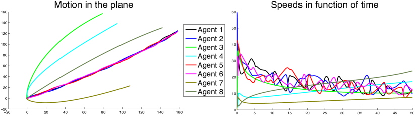
Figure 16: Space evolution and speeds of the uncontrolled system.

Though we can not infer the divergence of the system from this finite-time simulation, the portrayed situation seems far from going towards a flocking behavior. The only agents which seem to flock are Agent 1, Agent 2, Agent 5 and Agent 6 (resp. black, blue, red and magenta trajectories), as it is also visible by the corresponding speed graph, in which the speed of each agent is adjusted to the one of the other agents.

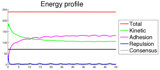
Figure 17: Energy profile of the uncontrolled system.

Figure 17 shows that the total energy $E$ (the red line) is constant and far away from the consensus threshold $\vartheta$ (black line). The increase in the distances between particles is reflected in an increase in the adhesion potential energy (the one due to $a$, see (38)) and in a decrease in the repulsive one (due to $f$).

If instead we apply our sparse control strategy with $M=35$ on the same system with the same initial conditions, the situation gets immediately far better from a consensus point of view, as Figure 18 witnesses.

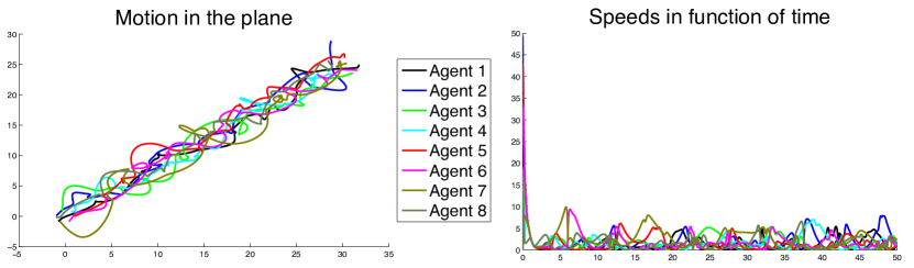
Figure 18: Space evolution and speeds of the controlled system.

The spatial evolution graph shows a braid movement which resembles a pattern near to flocking as it is commonly interpreted. The action of our control is evident from the energy profile of the system, portrayed in Figure 19, where the total energy is driven below the threshold in a very short time. The fall of the total energy is mainly due to its kinetic part (the green line), which is the only one directly affected by our control strategy. The sharp decrease of the kinetic energy is also witnessed in the graph showing the modulus of the speeds, where, after a quick, strong brake at the beginning, they stabilize at a very low level.

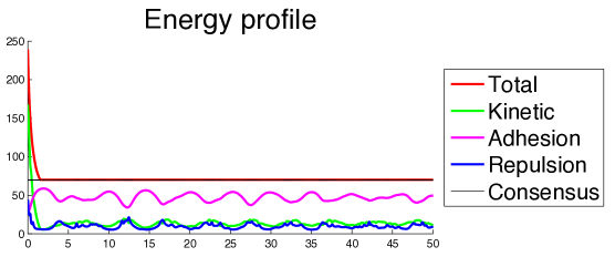
Figure 19: Energy profile of the controlled system.

Tuning the parameter $M$

The second case study takes into account a system with a weaker communication rate than before ($\beta=1.02$) and with a different form of the repulsive function ($p=1.1$), and we apply on it our control strategy with several values for $M$.

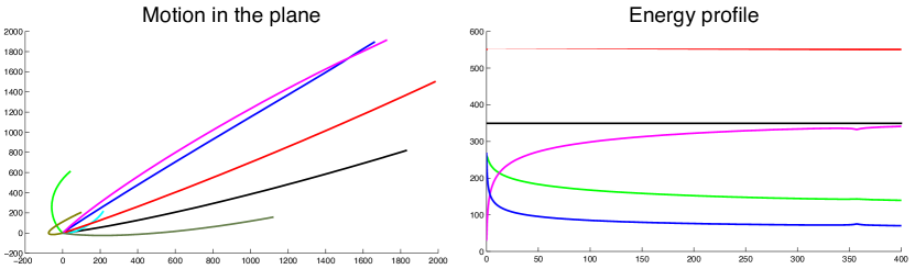
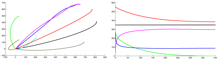
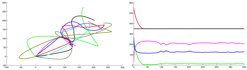
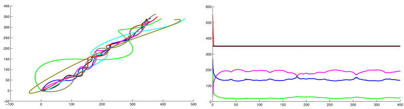
Figure 20: Spatial evolutions (left) and relative energy profiles (right). From top to bottom: $M=0,M=0.1,M=1,M=10$. The colors in the left column stand for: total energy (red), consensus region (black), adhesion energy (magenta), repulsion energy (blue), kinetic energy (green).

The top-left corner of Figure 20 is the uncontrolled system: it seems legitimate to suppose that it is very unlikely that the system will converge to consensus, especially looking at its energy profile graph (top-right corner of Figure 20), which shows an increase in the adhesion potential energy, phenomenon associated to an increase in the distance between particles, as already pointed out. In the second line we see the spatial evolution graph of the same system but with the sparse control strategy acting with parameter $M=0.1$, where the agents are starting to converge to consensus, as is also evident in their energy profile. The two bottom lines of Figure 20 display the action of controls with $M=1$ and $M=10$, respectively. It is clear how the situation goes better as $M$ increases, which is due to the fact that the threshold is reached in shorter time (see the relative energy profile).

The right column of Figure 20 also clearly confirms the behavior of the decay rate of the energy as a function of $M$, as predicted by our analysis: $E(t)$ decreases as $e^{-kMt}$, for a certain constant $k>0$.

It is interesting to notice that convergence to the consensus region occurs even if the hypothesis $(b)$ of Theorem 7.1 is not met, i.e., $\vartheta$ is very far away from $E(0)$, as it is likely to be a sub-optimal sufficient condition. Indeed, in all the case studies above

$$c=\exp\left(-\frac{2\sqrt{3}}{9}\frac{M\left\|{\overline{v}(0)}\right\|^{3}}{E(0)\sqrt{E(0)}\left(\Lambda\sqrt{E(0)}+\frac{M}{N}\right)}\right)\approx 1,$$

but, nonetheless, we were able to steer the system to consensus in finite time.

A counterexample to unconditional sparse controllability

The last numerical experiment we report shows that in certain pathological situations the sparse control strategy can fail to steer a Cucker-Dong systems to consensus.

We consider $N=2$ agents in dimension $d=2$ and choose the interaction parameters as $H=1$, $\beta=2$, $p=1.1$, $\Lambda=0$, and $M=1$. In this situation, the force balance $f-a$ is completely in favor of the repulsive force, as Figure 21 shows: this means that, regardless of the mutual positions of the agents, they shall always be repelled from each other.

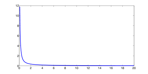
Figure 21: Sum of the attraction and repulsion forces $h(r)=f(r)-a(r)$ as a function of the distance $r>0$ in the case study of Section 7.3

If we exert the sparse control strategy, the only result that we obtain is to freeze the agents where they are. Indeed, Figure 22 shows that the agents’ speeds are rapidly reduced to values close to 0 as an effect of the control (also visible in the energy profile from the trajectory of the kinetic energy), but the total energy stays far away from the consensus region (the black line). The picture makes very clear that the sparse feedback control does not affect the potential energy of the system, as the sum of the adhesion and repulsion energies stays constant in time.

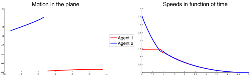
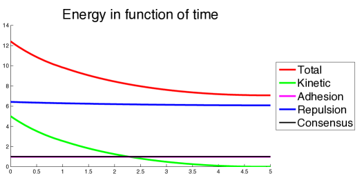
Figure 22: Space evolution, speeds and energy profile of the system considered in Section 7.3.

Furthermore, notice that, as soon as we shut down the control, the two agents will start to move again in opposite directions (very slowly, since the energy of a system without control stays constant), hence not only the total energy remains above the threshold, but also the system is not in consensus.

However, it must be observed that the control strategy fails in this situation due to the peculiar nature of the system. As a matter of fact, being the force balance strictly repulsive, the trajectories of any solution will never remain cohesive. This leaves open the question whether there exist “non-pathological” instances of the Cucker-Dong model (in the sense that their solutions are not doomed to diverge regardless of the initial condition) for which the sparse control strategy does not work.

- [1] S. M. Ahn and S.-Y. Ha. Stochastic flocking dynamics of the Cucker-Smale model with multiplicative white noises. J. Math. Phys., 51(10):103301, 2010.
- [2] G. Albi, M. Bongini, E. Cristiani, and D. Kalise. Invisible sparse control of self-organizing agents leaving unknown environments. To appear in SIAM J. Appl. Math., 2015.
- [3] F. Arvin, J. C. Murray, L. Shi, C. Zhang, and S. Yue. Development of an autonomous micro robot for swarm robotics. In Proceedings of the IEEE International Conference on Mechatronics and Automation (ICMA), pages 635–640. IEEE, 2014.
- [4] P. Bak. How nature works: the science of self-organized criticality. Springer Science & Business Media, 2013.
- [5] M. Ballerini, N. Cabibbo, R. Candelier, A. Cavagna, E. Cisbani, I. Giardina, V. Lecomte, A. Orlandi, G. Parisi, A. Procaccini, M. Viale, and V. Zdravkovic. Interaction ruling animal collective behavior depends on topological rather than metric distance: Evidence from a field study. P. Natl. Acad. Sci. USA, 105(4):1232–1237, 2008.
- [6] S. Battiston, D. Delli Gatti, M. Gallegati, B. Greenwald, and J. Stiglitz. Liaisons dangereuses: Increasing connectivity, risk sharing, and systemic risk. J. Econ. Dyn. Control, 36(8):1121–1141, 2012.
- [7] M. Bongini. Sparse Optimal Control of Multiagent Systems. PhD thesis, Technische Universität München, 2016.
- [8] M. Bongini and M. Fornasier. Sparse stabilization of dynamical systems driven by attraction and avoidance forces. Netw. Heterog. Media, 9(1):1–31, 2014.
- [9] M. Bongini, M. Fornasier, F. Frölich, and L. Hagverdi. Sparse control of force field dynamics. In International Conference on NETwork Games, COntrol and OPtimization, October 2014.
- [10] M. Bongini, M. Fornasier, O. Junge, and B. Scharf. Sparse control of alignment models in high dimension. Netw. Heterog. Media, 10(3):647–697, 2015.
- [11] M. Bongini, M. Fornasier, and D. Kalise. (Un)conditional consensus emergence under perturbed and decentralized feedback controls. Discrete Contin. Dyn. Syst., 35(9):4071–4094, 2015.
- [12] A. Borzì and S. Wongkaew. Modeling and control through leadership of a refined flocking system. Math. Models Methods Appl. Sci., 25(02):255–282, 2015.
- [13] S. Camazine, J.-L. Deneubourg, N. Franks, J. Sneyd, G. Theraulaz, and E. Bonabeau. Self-organization in biological systems. Princeton University Press, 2002.
- [14] E. J. Candès, J. K. Romberg, and T. Tao. Stable signal recovery from incomplete and inaccurate measurements. Comm. Pure Appl. Math., 59(8):1207–1223, 2006.
- [15] M. Caponigro, M. Fornasier, B. Piccoli, and E. Trélat. Sparse stabilization and optimal control of the Cucker-Smale model. Math. Control Relat. Fields, 3(4):447–466, 2013.
- [16] M. Caponigro, M. Fornasier, B. Piccoli, and E. Trélat. Sparse stabilization and control of alignment models. Math. Models Methods Appl. Sci., 25(03):521–564, 2015.
- [17] J. A. Carrillo, Y.-P. Choi, and M. Hauray. The derivation of swarming models: mean-field limit and Wasserstein distances. In Collective Dynamics from Bacteria to Crowds, pages 1–46. Springer, 2014.
- [18] J. A. Carrillo, M. R. D’Orsogna, and V. Panferov. Double milling in self-propelled swarms from kinetic theory. Kinet. Relat. Models, 2(2):363–378, 2009.
- [19] J. A. Carrillo, M. Fornasier, J. Rosado, and G. Toscani. Asymptotic flocking dynamics for the kinetic Cucker-Smale model. SIAM J. Math. Anal., 42(1):218–236, 2010.
- [20] J. A. Carrillo, M. Fornasier, G. Toscani, and F. Vecil. Particle, kinetic, and hydrodynamic models of swarming. In Mathematical Modeling of Collective Behavior in Socio-Economic and Life Sciences, Modeling and Simulation in Science, Engineering and Technology, pages 297–336. Birkhäuser Boston, 2010.
- [21] E. Casas, C. Clason, and K. Kunisch. Approximation of elliptic control problems in measure spaces with sparse solutions. SIAM J. Control Optim., 50(4):1735–1752, 2012.
- [22] Y.-L. Chuang, M. R. D’Orsogna, D. Marthaler, A. L. Bertozzi, and L. S. Chayes. State transitions and the continuum limit for a 2D interacting, self-propelled particle system. Phys. D, 232(1):33–47, 2007.
- [23] F. R. K. Chung. Spectral graph theory, volume 92. American Mathematical Society, 1997.
- [24] C. Clason and K. Kunisch. A measure space approach to optimal source placement. Comput. Optim. Appl., 53(1):155–171, 2012.
- [25] M. A. Cohen and S. Grossberg. Absolute stability of global pattern formation and parallel memory storage by competitive neural networks. IEEE Trans. Syst., Man, Cybern., Syst., 13(5):815–826, 1983.
- [26] J. Cortés and F. Bullo. Coordination and geometric optimization via distributed dynamical systems. SIAM J. Control Optim., 44(5):1543–1574, 2005.
- [27] I. D. Couzin and N. R. Franks. Self-organized lane formation and optimized traffic flow in army ants. P. Roy. Soc. Lond. B Bio., 270(1511):139–146, 2003.
- [28] I. D. Couzin, J. Krause, N. R. Franks, and S. A. Levin. Effective leadership and decision-making in animal groups on the move. Nature, 433:513–516, 2005.
- [29] A. J. Craig and I. Flügge-Lotz. Investigation of optimal control with a minimum-fuel consumption criterion for a fourth-order plant with two control inputs; synthesis of an efficient suboptimal control. J. Fluids Eng., 87(1):39–58, 1965.
- [30] E. Cristiani, B. Piccoli, and A. Tosin. Modeling self-organization in pedestrians and animal groups from macroscopic and microscopic viewpoints. In Mathematical modeling of collective behavior in socio-economic and life sciences, pages 337–364. Springer, 2010.
- [31] E. Cristiani, B. Piccoli, and A. Tosin. Multiscale modeling of granular flows with application to crowd dynamics. Multiscale Model. Simul., 9(1):155–182, 2011.
- [32] F. Cucker and J.-G. Dong. A general collision-avoiding flocking framework. IEEE Trans. Automat. Control, 56(5):1124–1129, 2011.
- [33] F. Cucker and J.-G. Dong. A conditional, collision-avoiding, model for swarming. Discrete Contin. Dynam. Systems, 34(3):1009–1020, 2014.
- [34] F. Cucker and S. Smale. Emergent behavior in flocks. IEEE Trans. Automat. Control, 52(5):852–862, 2007.
- [35] F. Cucker and S. Smale. On the mathematics of emergence. Jpn. J. Math., 2(1):197–227, 2007.
- [36] F. Cucker, S. Smale, and D. Zhou. Modeling language evolution. Found. Comput. Math., 4(5):315–343, 2004.
- [37] S. Currarini, M. O. Jackson, and P. Pin. An economic model of friendship: Homophily, minorities, and segregation. Econometrica, 77(4):1003–1045, 2009.
- [38] F. Dalmao and E. Mordecki. Cucker-Smale flocking under hierarchical leadership and random interactions. SIAM J. Appl. Math., 71(4):1307–1316, 2011.
- [39] J. Dickinson. Animal social behavior. In Encyclopaedia Britannica Online. Encyclopaedia Britannica Inc., 2016.
- [40] D. L. Donoho. Compressed sensing. IEEE Trans. Inform. Theory, 52(4):1289–1306, 2006.
- [41] M. R. D’Orsogna, Y.-L. Chuang, A. L. Bertozzi, and L. S. Chayes. Self-propelled particles with soft-core interactions: patterns, stability, and collapse. Phys. Rev. Lett., 96(10):104302, 2006.
- [42] Y. Eldar and H. Rauhut. Average case analysis of multichannel sparse recovery using convex relaxation. IEEE Trans. Inform. Theory, 56(1):505–519, 2010.
- [43] J. A. Fax and R. M. Murray. Information flow and cooperative control of vehicle formations. IEEE Trans. Automat. Control, 49(9):1465–1476, 2004.
- [44] A. F. Filippov. Differential Equations with Discontinuous Righthand Sides. Kluwer Academic Publishers, 1988.
- [45] M. Fornasier and H. Rauhut. Recovery algorithms for vector-valued data with joint sparsity constraints. SIAM J. Numer. Anal., 46(2):577–613, 2008.
- [46] M. Fornasier and H. Rauhut. Handbook of Mathematical Methods in Imaging, chapter Compressive Sensing, pages 187–228. Springer-Verlag, 2010.
- [47] S.-Y. Ha, T. Ha, and J.-H. Kim. Emergent behavior of a Cucker-Smale type particle model with nonlinear velocity couplings. IEEE Trans. Automat. Control, 55(7):1679–1683, 2010.
- [48] S.-Y. Ha, J.-G. Liu, et al. A simple proof of the Cucker-Smale flocking dynamics and mean-field limit. Commun. Math. Sci., 7(2):297–325, 2009.
- [49] G. Hardin. The tragedy of the commons. Science, 162(3859):1243–1248, 1968.
- [50] J. Haskovec. A note on the consensus finding problem in communication networks with switching topologies. Appl. Anal., 94(5):991–998, 2015.
- [51] R. Hegselmann and U. Krause. Opinion dynamics and bounded confidence models, analysis, and simulation. J. Artif. Soc. Soc. Simulat., 5(3), 2002.
- [52] R. Herzog, G. Stadler, and G. Wachsmuth. Directional sparsity in optimal control of partial differential equations. SIAM J. Control Optim., 50(2):943–963, 2012.
- [53] E. F. Keller and L. A. Segel. Initiation of slime mold aggregation viewed as an instability. J. Theor. Biol., 26(3):399–415, 1970.
- [54] A. Kirman, S. Markose, S. Giansante, and P. Pin. Marginal contribution, reciprocity and equity in segregated groups: Bounded rationality and self-organization in social networks. J. Econ. Dyn. Control, 31(6):2085–2107, 2007.
- [55] A. Koch and D. White. The social lifestyle of myxobacteria. Bioessays 20, pages 1030–1038, 1998.
- [56] S. Mallat. A wavelet tour of signal processing: the sparse way. Academic press, 2008.
- [57] M. McPherson, L. Smith-Lovin, and J. M. Cook. Birds of a feather: Homophily in social networks. Annu. Rev. Sociol., pages 415–444, 2001.
- [58] B. Mohar. The Laplacian spectrum of graphs. In Y. Alavi, G. Chartrand, O. R. Oellermann, and A. J. Schwenk, editors, Graph theory, Combinatorics, and Applications, volume 2, pages 871–898. Wiley, 1991.
- [59] L. Moreau. Stability of multiagent systems with time-dependent communication links. IEEE Trans. Automat. Control, 50(2):169–182, 2005.
- [60] S. Motsch and E. Tadmor. Heterophilious dynamics enhances consensus. SIAM Rev., 56(4):577–621, 2014.
- [61] J. F. Nash. Equilibrium points in -person games. Proc. Natl. Acad. Sci. USA, 36(1):48–49, 1950.
- [62] H. Niwa. Self-organizing dynamic model of fish schooling. J. Theor. Biol., 171:123–136, 1994.
- [63] F. Paganini, J. Doyle, and S. Low. Scalable laws for stable network congestion control. In Proceedings of the 40th IEEE Conference on Decision and Control, volume 1, pages 185–190. IEEE, 2001.
- [64] J. Parrish and L. Edelstein-Keshet. Complexity, pattern, and evolutionary trade-offs in animal aggregation. Science, 294:99–101, 1999.
- [65] J. Parrish, S. Viscido, and D. Gruenbaum. Self-organized fish schools: An examination of emergent properties. Biol. Bull., 202:296–305, 2002.
- [66] L. Perea, P. Elosegui, and G. Gómez. Extension of the Cucker-Smale control law to space flight formations. J. Guid. Control Dynam., 32(2):527–537, 2009.
- [67] B. Perthame. Transport Equations in Biology. Basel: Birkhäuser, 2007.
- [68] L. Petrovic, M. Henne, and J. Anderson. Volumetric Methods for Simulation and Rendering of Hair. Technical report, Pixar Animation Studios, 2005.
- [69] C. W. Reynolds. Flocks, herds and schools: A distributed behavioral model. ACM SIGGRAPH Computer Graphics, 21(4):25–34, 1987.
- [70] W. Romey. Individual differences make a difference in the trajectories of simulated schools of fish. Ecol. Model., 92:65–77, 1996.
- [71] J. Shen. Cucker-Smale flocking under hierarchical leadership. SIAM J. Appl. Math., 68(3):694–719, 2007.
- [72] M. B. Short, M. R. D’Orsogna, V. B. Pasour, G. E. Tita, P. J. Brantingham, A. L. Bertozzi, and L. B. Chayes. A statistical model of criminal behavior. Math. Models Methods Appl. Sci., 18(suppl.):1249–1267, 2008.
- [73] G. Stadler. Elliptic optimal control problems with -control cost and applications for the placement of control devices. Comput. Optim. Appl., 44(2):159–181, 2009.
- [74] H. G. Tanner, A. Jadbabaie, and G. J. Pappas. Flocking in fixed and switching networks. IEEE Trans. Automat. Control, 52(5):863–868, 2007.
- [75] J. Toner and Y. Tu. Long-range order in a two-dimensional dynamical xy model: How birds fly together. Phys. Rev. Lett., 75:4326–4329, 1995.
- [76] T. Vicsek, A. Czirók, E. Ben-Jacob, I. Cohen, and O. Shochet. Novel type of phase transition in a system of self-driven particles. Phys. Rev. Lett., 75(6):1226, 1995.
- [77] T. Vicsek and A. Zafeiris. Collective motion. Phys. Rep., 517(3):71–140, 2012.
- [78] J. von Neumann and O. Morgenstern. Theory of Games and Economic Behavior. Princeton University Press, 1944.
- [79] G. Wachsmuth and D. Wachsmuth. Convergence and regularization results for optimal control problems with sparsity functional. ESAIM Control Optim. Calc. Var., 17(3):858–886, 2011.
- [80] G. Weisbuch, G. Deffuant, F. Amblard, and J.-P. Nadal. Meet, discuss, and segregate! Complexity, 7(3):55–63, 2002.
- [81] S. Wongkaew, M. Caponigro, and A. Borzì. On the control through leadership of the Hegselmann–Krause opinion formation model. Math. Models Methods Appl. Sci., 25(03):565–585, 2015.
- [82] C. Yates, R. Erban, C. Escudero, L. Couzin, J. Buhl, L. Kevrekidis, P. Maini, and D. Sumpter. Inherent noise can facilitate coherence in collective swarm motion. Proceedings of the National Academy of Sciences, 106:5464–5469, 2009.