Numerical stabilization of entanglement computation in auxiliary field quantum Monte Carlo simulations of interacting many-fermion systems

Abstract

In the absence of a fermion sign problem, auxiliary field (or determinantal) quantum Monte Carlo (DQMC) approaches have long been the numerical method of choice for unbiased, large-scale simulations of interacting many-fermion systems. More recently, the conceptual scope of this approach has been expanded by introducing ingenious schemes to compute entanglement entropies within its framework. On a practical level, these approaches however suffer from a variety of numerical instabilities that have largely impeded their applicability. Here we report on a number of algorithmic advances to overcome many of these numerical instabilities and significantly improve the calculation of entanglement measures in the zero-temperature projective DQMC approach, ultimately allowing to reach similar system sizes as for the computation of conventional observables. We demonstrate the applicability of this improved DQMC approach by providing an entanglement perspective on the quantum phase transition from a magnetically ordered Mott insulator to a band insulator in the bilayer square lattice Hubbard model at half filling.

I Introduction

In statistical physics, quantum Monte Carlo (QMC) simulations are a mainstay of the numerical characterization of quantum many-body systems Gubernatis et al. (2016). Revered for their ability to provide unbiased, numerically exact results even in the strong coupling regime, they provide valuable insight and theoretical guidance where analytical approaches such as mean-field or perturbative calculations often fail. World-line approaches such as the stochastic series expansion (SSE) Sandvik (1999) (used in combination with non-local update schemes Syljuåsen and Sandvik (2002); Alet et al. (2005); Troyer et al. (2003)) or the continuous-time formulation of the worm algorithm Prokof’ev et al. (1998) have basically solved unfrustrated bosonic systems from a numerical perspective. For fermionic many-body systems, the situation is somewhat more delicate with the infamous fermion sign problem Hirsch et al. (1982); Loh et al. (1990) thwarting the polynomial efficiency of the approach for a range of problems, i.e. its power-law scaling with system size and inverse temperature. Nevertheless, one should not overlook that there are a number of fermionic quantum many-body systems that do not suffer from the fermion sign problem and at the same time exhibit interesting physics arising solely from the fermionic nature of its constituents. This includes, for instance, the formation of superconductivity in microscopic models of nearly antiferromagnetic metals Berg et al. (2012); Schattner et al. (2016), the emergence of topological order in Kane-Mele-Hubbard models Bercx et al. (2014); Hohenadler et al. (2014); Parisen Toldin et al. (2015), or fermionic quantum critical phenomena in Dirac matter Wang et al. (2014a); Li et al. (2015); Motruk et al. (2015); Capponi and Läuchli (2015); Broecker and Trebst (2016) or Z₂ gauge field coupled fermion systems Assaad and Grover ; Gazit et al. . Large-scale lattice models of all these fermionic systems have been simulated using DQMC simulations in the past three years, typically with an emphasis on the statistical measurement of observables such as order parameters, correlation functions, or topological invariants. At the same time, conceptual advancements have paved the way to calculate entanglement measures such as Rényi entropies or entanglement spectra within the framework of DQMC simulations Grover (2013); Broecker and Trebst (2014); Assaad et al. (2014); Assaad (2015), in step with similar developments for their bosonic world-line counterparts Hastings et al. (2010); Herdman et al. (2014). However, the practical use of these entanglement computations has so far been impeded by a number of numerical instabilities arising deep within the DQMC technique. The purpose of the manuscript at hand is to give a detailed account as to how to overcome these numerical insufficiencies and bring the computation of entanglement measures en par with conventional observables. Our algorithmic improvements focus on the calculation of Rényi entropies using an adaptation of the replica scheme Holzhey et al. (1994); Calabrese and Cardy (2004) to the DQMC approach Broecker and Trebst (2014). The numerical stabilization of its computation includes a variety of algorithmic steps ranging from linear algebra aspects such as the inversion of seemingly singular matrices and technical tricks such the inclusion of an artificial chemical potential, which is shown to control the condition numbers of the underlying linear algebra algorithms, to more DQMC specific aspects such as the optimal choice of Hubbard-Stratonovich transformation and respective auxiliary fields. Beyond the numerical stabilization we provide a detailed discussion of the convergence behavior of our enhanced algorithm. Finally, to illustrate the performance of the technical improvements laid out in this manuscript, we apply our DQMC + replica scheme framework to provide an entanglement perspective on the quantum phase transition between an antiferromagnetically ordered Mott insulator and a featureless band insulator in the bilayer Hubbard model on the square lattice.

The remainder of the manuscript is organized as follows. We start with a brief review of the general auxiliary field quantum Monte Carlo approach in Sec. II where we put a particular emphasis on those aspects where numerical instabilities typically arise and how they are dealt with in the conventional algorithm Blankenbecler et al. (1981); dos Santos (2003); Assaad and Evertz (2008) that is used to compute correlation functions at finite temperatures. We then turn to the replica scheme and discuss its conceptual adaptation to the DQMC framework in Sec. III. The main results of the manuscript are provided in Sec. IV where we discuss the numerical stabilization for the calculation of Rényi entropies, followed by a discussion of the optimal choice of Hubbard-Stratonovich transformation in Sec. IV.3 and the overall convergence behavior of the algorithm in Sec. IV.4. The application of the so-improved DQMC approach to the quantum phase transition in the bilayer Hubbard model is presented in Sec. V. We close with a discussion in Sec. VI.

II Auxiliary field quantum Monte Carlo

We start our discussion with a brief recapitulation of the basics of the DQMC method Blankenbecler et al. (1981). We will primarily discuss its finite-temperature formulation and only touch on some of the aspects of the alternative zero-temperature projective scheme. This choice of focus is motivated by the fact that the algorithm for the computation of ground-state entanglement properties is conceptually much closer to the finite-temperature approach than the projective scheme. Readers looking for a more exhaustive introduction to DQMC approaches are referred to the review articles in Refs. dos Santos, 2003; Assaad and Evertz, 2008.

II.1 Conceptual formalism

From a conceptual perspective, the goal of determinantal quantum Monte Carlo approaches is to sample the partition function

$$Z=\text{Tr}\,{e^{-\beta\hat{H}}}\,.$$ (1)

for a given lattice Hamiltonian $\hat{H}$ in the grand-canonical ensemble and to evaluate finite-temperature expectation values of correlation functions along the way. The first step in accomplishing this is to perform a Trotter-Suzuki decomposition, discretizing the inverse temperature or imaginary time into $N_{\tau}$ time slices of size $\Delta\tau=\beta/N_{\tau}$. The investigated Hamiltonians are typically of the form $\hat{H}=\hat{K}+\hat{V}$ with a non-interacting, quadratic part $\hat{K}$ and an interacting, quartic part $\hat{V}$, respectively. By making use of the Baker-Campbell-Hausdorff formula, one can split the sum in the exponential into a product of exponentials and keep only the lowest order term

$$Z=\text{Tr}\,\prod\limits_{\tau=1}^{N_{\tau}}e^{-\Delta\tau\hat{K}}e^{-\Delta\tau\hat{V}}+\mathcal{O}(\Delta\tau^{2})\,.$$ (2)

Ignoring the higher orders introduces an error of size $\mathcal{O}(\Delta\tau^{2})$ that can be considered negligible if $\Delta\tau$ is sufficiently small. To evaluate the interaction part, we apply a Hubbard-Stratonovich transformation Stratonovich (1957); Hubbard (1959) on each time slice and each term in the interaction operator reducing quartic to quadratic operators at the cost of introducing an auxiliary field that we denote by $s(\tau,j)$, with $\tau$ being the time slice and $j$ the index indicating the decoupled term of the interaction operator. After this Hubbard-Stratonovich transformation, we end up with a system of free fermions coupled to the auxiliary field via an interaction $V(s,\tau)$ that depends on the auxiliary field configuration and the time slice in imaginary time. The operators $\hat{K}$ and $\hat{V}(s,\tau)$ are now simply one-particle operators and can be written out in their matrix form K and $\textsf{{V}}(s,\tau)$, respectively, so that the partition sum is given as

$$Z =\sum\limits_{s(\tau,j)}\text{Tr}\,\prod\limits_{\tau=1}^{N_{\tau}}e^{-\Delta\tau\textsf{{K}}}e^{-\Delta\tau\textsf{{V}}(s,\tau)}$$

$$=\sum\limits_{s(\tau,j)}\text{Tr}\,\prod\limits_{\tau=1}^{N_{\tau}}\textsf{{B}}(s,\tau)$$

where $\textsf{{B}}(s,\tau)$ denotes the matrix product of the hopping matrix and the decoupled interaction matrix for a given time slice $\tau$ and a given auxiliary field configuration $s$. Let us introduce some notation that we will use throughout the following. First, in favor of a clearer notation, we will the drop the auxiliary field argument $s$, since we will focus on calculating objects for a fixed configuration. We define a partial product of slice matrices starting at time slice $\tau$ and ending at time slice $\tau^{\prime}$ as

$$B(\tau^{\prime},\tau)=\prod\limits_{i=\tau}^{\tau^{\prime}}\textsf{{B}}(i)\,,$$ (4)

The full product over all time slices is denoted as

$$\mathcal{B}(\tau=1)=\prod\limits_{i=1}^{N_{\tau}}\textsf{{B}}(i)\,,$$ (5)

where the label $\tau$ in the latter indicates the starting point for the matrix product. If $\tau\neq 1$, then the corresponding matrix product should be viewed as cyclically permuted by $\tau-1$ elements, a perspective which we will later use when accessing equal-time Green’s functions at different imaginary time slices. Using this notation, we may write the partition sum in the following concise way

$$Z=\sum\limits_{\{s(\tau,j)\}}\text{Tr}\,\,\mathcal{B}(\tau=1)\,.$$ (6)

At this point, it should be noted that the partition sum still contains a trace over all fermion states and over all auxiliary field configurations $s(\tau,j)$. We can, however, integrate out the free fermions, resulting in one determinant per auxiliary field and fermion configuration. It can further be shown dos Santos (2003); Assaad and Evertz (2008) that the sum of determinants reduces to a single determinant quantifying the electron contribution to the partition sum for any given configuration of the auxiliary field. This allows to reformulate the original partition sum (1) in terms of determinants as

$$Z=\sum\limits_{\{s(\tau,j)\}}\det{(1+\mathcal{B}(\tau))}\,.$$ (7)

A central object of quantum statistical physics is the equal-time Green’s function $G(\tau)$, which is easily accessible in the DQMC algorithm with its matrix form related to the above determinants via

$$G(\tau)=(1+\mathcal{B}(\tau))^{-1}\,.$$ (8)

The equal-time Green’s function not only provides valuable access to correlation functions, it also plays a crucial role in devising an efficient updating procedure of the auxiliary field configurations sampled at the heart of the Monte Carlo approach. For details we again refer to the literature dos Santos (2003); Assaad and Evertz (2008).

II.2 Numerical implementation

Any practical implementation of the algorithm described above typically faces two problems, both related to the underlying linear algebra: (i) the evaluation of the matrix product (5) is found to be numerically unstable Bai et al. (2011) and (ii) the resulting matrix $\mathcal{B}(\tau)$ turns out to be ill-conditioned, which hampers both the calculation of the Monte Carlo transition probabilities as well as the evaluation of the equal-time Green’s function and any observables derived from it. The condition number of the matrix product increases with increasing hopping strength and increasing inverse temperature, respectively and may increase or decrease with increasing interaction strength depending on the type of Hubbard-Stratonovich transformation.

Stabilizing a matrix product of the form (5) is a well understood procedure in numerical mathematics. The idea is to perform either a rank revealing QR or a singular value decomposition (SVD) after a certain number of multiplications $m$, typically chosen small enough such that this shorter product remains exact up to machine precision. By making use of one of the decompositions one recasts a given matrix $M$ into a product $M=UDT$, where $U$ is typically unitary, $D$ is a diagonal matrix that contains the information about the inherent scales of the matrix (e.g. in the form of its singular value spectrum), and $T$ is either unitary (SVD) or triangular (QR decomposition). Independent of the specific decomposition algorithm, we will refer to the values of the diagonal matrix $D$ as the singular values. To stabilize the computation of the matrix product (5), we divide the imaginary time interval into $N_{m}$ groups of $m$ time slices representing a segment of length $\Delta=m\cdot\tau$ in imaginary time that encompasses $m$ slice matrices $\textsf{{B}}(i)$. After the multiplication and decomposition of the first $m$ matrices into $U_{1}D_{1}T_{1}$, the next set of matrices is then multiplied only to $U_{1}$, before $D_{1}$ is multiplied from the right and the resulting product is decomposed again, i.e.

$$\left(\left(\prod\limits_{i=m+1}^{2m}\textsf{{B}}(i)\cdot U_{1}\right)D_{1}\right)T_{1}=U_{2}D_{2}(TT_{1})=U_{2}D_{2}T_{2}\,.$$ (9)

This procedure is repeated until all slice matrices are incorporated into the $UDT$ decomposition. Note that we will use all the incomplete, intermediate results at a later point so they will be stored in memory. We refer to this set of matrices, $\{\{U_{i}\},\{D_{i}\},\{T_{i}\}\}$, as the stack.

The determinant that gives the weight of a specific configuration of the auxiliary field is given as

$$\det{\left(\mathbb{1}+\mathcal{B}(\tau)\right)}=\det{\left(\mathbb{1}+UDT\right)}\,,$$ (10)

and the equal-time Green’s function as

$$G(\tau)=\left(\mathbb{1}+\mathcal{B}(\tau)\right)^{-1}=\left(\mathbb{1}+UDT\right)^{-1}\,.$$ (11)

The addition of the identity matrix, although seemingly simple, requires careful attention to ensure an accurate calculation of the determinant and the Green’s function. This problem is solved by separating the diagonal matrix $D$ from the auxiliary matrices $U$ and $T$ before the resulting matrix is decomposed yet again:

$$\left(\mathbb{1}+UDT\right)=U\left(U^{-1}T^{-1}+D\right)T=\left(UU^{\prime}\right)D^{\prime}\left(T^{\prime}T\right)\,.$$ (12)

The weight, i.e. the determinant, can then easily be read off as the product of the diagonal entries of $D^{\prime}$. It should be noted that in practice one would calculate the logarithm of the determinant to avoid numerical overflow and rounding errors.

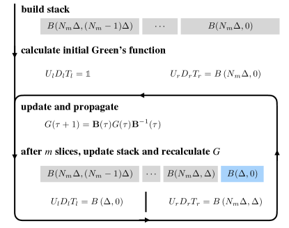
Figure 1: Flow diagram of the basic DQMC algorithm. Shaded in grey is the initial build up of the stack of decomposed matrix products. This is used to calculate the Green’s function which is subsequently updated and propagated in imaginary time before updating the stack and recalculating the Green’s function from the stack to ensure stability. The slice product shaded in red has to be recalculated from scratch because it contains auxiliary field values that were updated in the Monte Carlo procedure. Subsequent slice products will the respective preceding $U$ matrix as a starting point for the recalculation.

We already mentioned that the Green’s function at a given imaginary time $\tau$ is also used in the updating procedure of the auxiliary field for the corresponding time slice, which means that we need to have access to the Green’s function at each time slice. One option would be to recalculate the Green’s function at every time slice from scratch, but that is numerically very expensive. Instead, one may propagate the Green’s function along imaginary time by virtue of

$$G(\tau+1)=\textsf{{B}}(\tau)G(\tau)\textsf{{B}}^{-1}(\tau)\,.$$ (13)

This equation suggests that we have to calculate the Green’s function only once, e.g. at $\tau=1$, and then continue propagating the Green’s function along imaginary time updating the appropriate auxiliary field degrees of freedom. However, the propagation suffers from the same problem as the build up of the matrix product (5) itself and is stable only for a few steps. In practice, we assume the number of stable propagation steps $N_{\text{prop}}$ to be equal to the number of slices $m$ making up groups of B-matrices. In general, this number can be determined by considering the difference between the propagated Green’s function and the recalculated one after $m$ propagations have taken place. The element-wise relative deviation

$$\delta_{ij}=2\cdot\dfrac{\left|G^{\text{recalculated}}_{ij}-G^{\text{propagated}}_{ij}\right|}{\left|G^{\text{recalculated}}_{ij}+G^{\text{propagated}}_{ij}\right|}$$ (14)

between the two should be small enough, such that the update probabilities and measurements are not seriously affected. Therefore, one typically focuses on comparing only those matrix elements that are used in the updating and measurement procedure. For those imaginary time slices where the Green’s function has to be recalculated from scratch, one can greatly facilitate its calculation by making use of the matrix products saved in the stack.

We summarize the basic DQMC algorithm in the flow diagram provided in Fig. 1.

III The replica scheme

To characterize and quantify the entanglement in a many-fermion system, we consider entanglement entropies Bekenstein (1973); Hawking (1975) calculated for a bipartition of the system into two complementary subsystems $A$ and $B$. Entanglement entropies have become a standard measure of entanglement for quantum many-body systems that can reveal valuable information about the principal nature of a quantum state Laflorencie (2016). Such a classification of quantum states is typically achieved by a careful scaling analysis of the entanglement entropies with system size, which reveals a dominant scaling with the length of the boundary of the bipartition Eisert et al. (2010) and several subleading contributions revealing e.g. the formation of macroscopic, long-range entanglement in topologically ordered systems Levin and Wen (2006); Kitaev and Preskill (2006), the formation of more conventionally symmetry-broken ordered states via a detection of the corresponding Goldstone modes Metlitski and Grover ; Kulchytskyy et al. (2015) or the existence of a Fermi surface via a logarithmic violation of the boundary law Wolf (2006); Gioev and Klich (2006). Technically, entanglement entropies are typically calculated in the form of Rényi entropies, which can be computed via the so-called replica scheme, a well-known procedure originally introduced in the context of quantum field theories Holzhey et al. (1994). In the following, we will quickly review how the replica scheme can be adapted to the framework of DQMC techniques.

III.1 Rényi entropies

Rényi entropies constitute a family of entanglement entropies calculated from the reduced density matrix $\rho_{A}=\text{Tr}_{B}\rho$ for a bipartition of the system into two complementary subsystems $A$ and $B$

$$S_{n}=\dfrac{1}{1-n}\log{\text{Tr}\,{\left(\rho_{A}^{n}\right)}}\,,$$ (15)

where the index $n$ is typically an integer number. This family of Rényi entropies includes the well-known von Neumann entropy $S=-\text{Tr}\,\left(\rho_{A}\log\rho_{A}\right)$, which is recovered in the limit of $n\rightarrow 1$. For the purpose of our numerical Monte Carlo simulations we will, however, consider only Rényi entropies with $n>1$, typically considering the case of the second Rényi entropy $n=2$, for which one can formulate the replica scheme Holzhey et al. (1994).

To quickly motivate and rederive this scheme let us start with the density matrix $\rho$ of the quantum many-body system at hand. In general, we can think of this density matrix as being subject to a normalization via a factor $\text{Tr}\,{\rho}$, which is, of course, unaffected if one takes the partial trace over degrees of freedom of part $B$. Inserting this into Eq. (15) gives

$$S_{n}=\dfrac{1}{1-n}\log{\dfrac{\text{Tr}\,{\left(\rho_{A}^{n}\right)}}{\left(\text{Tr}\,\rho\right)^{n}}}\,,$$ (16)

which we rewrite as the ratio of two partition sums

$$S_{n}=\dfrac{1}{1-n}\log{\dfrac{\mathcal{Z}[A,n,\beta]}{\mathcal{Z}^{n}}}\,,$$ (17)

with $\mathcal{Z}[A,n,\beta]=\text{Tr}\,{\left(\rho_{A}^{n}\right)}$ and $\mathcal{Z}^{n}=\left(\text{Tr}\,\rho\right)^{n}$, respectively. In the following, let us focus on the second Rényi entropy, i.e. $n=2$, for which the two equations above reduce to

$$S_{2}=-\log{\dfrac{\text{Tr}\,{\left(\rho_{A}^{2}\right)}}{\left(\text{Tr}\,\rho\right)^{2}}}=-\log{\dfrac{\mathcal{Z}[A,2,\beta]}{\mathcal{Z}^{2}}\equiv-\log{\dfrac{Z_{1}}{Z_{0}}}}\,.$$ (18)

Note that $\mathcal{Z}$ is the usual partition function, which we sample in conventional DQMC simulations to obtain numerical estimates of conventional observables such as, for instance, correlation functions. The second partition function $\mathcal{Z}[A,2,\beta]$ entering the above equation is a modified partition function, where part $B$ was traced out and the resulting reduced density matrix was squared ($n=2$) before the final trace over $A$ was taken. Associated to these partition functions are Green’s functions $G_{0}$ and $G_{1}$, respectively. Written out explicitly $\mathcal{Z}[A,2,\beta]$ takes the form

$$\text{Tr}\,_{A}\left(\rho_{A}^{\prime 2}\right) =\sum\limits_{\mathcal{A},\mathcal{A}^{\prime},\mathcal{B},\mathcal{B}^{\prime}}\left<\mathcal{A}{\mathcal{B}^{\prime}}\right|\rho^{\prime}\left|\mathcal{A}^{\prime}{\mathcal{B}^{\prime}}\right>\left<\mathcal{A}^{\prime}{\mathcal{B}}\right|\rho^{\prime}\left|\mathcal{A}\mathcal{B}\right>$$

$$\equiv\mathcal{Z}[A,2,\beta]\,.$$ (19)

Note that $\mathcal{Z}[A,2,\beta]$ is $\beta$-periodic in part $B$ which due to the squaring appears twice, once as $\mathcal{B}$ and once as $\mathcal{B}^{\prime}$, while part $A$ is $2\beta$-periodic and appears only once. These peculiar boundary conditions in imaginary time can best be understood when visualized in a world-line picture as shown in Fig. 2.

III.2 The replica scheme in DQMC simulations

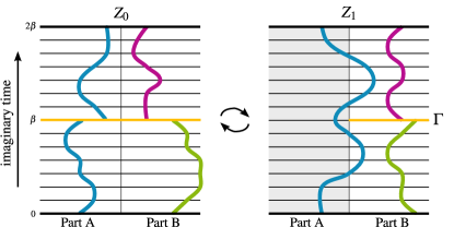
Figure 2: (Color online) Worldline representation of the two partition sums of (18). On the left side, the squared, regular partition function is depicted. Worldlines of particles are $\beta$-periodic, no matter what subsystem they originate from. The right hand side shows the modified partition sum that is $\beta$-periodic in part $B$ but $2\beta$-periodic in part $A$.

To adapt this replica scheme in DQMC simulations, we have previously shown Broecker and Trebst (2014) that one can “fold out” subsystems $B$ and $B^{\prime}$ and consider a modified Hamiltonian that explicitly depends on imaginary time and takes the form

$$\widetilde{\mathcal{H}}(\tau)=\mathcal{H}_{AB}\;\Theta(\tau)\;\Theta(\beta-\tau)+\mathcal{H}_{AB^{\prime}}\;\Theta(\tau-\beta)\;\Theta(2\beta-\tau)\,.$$ (20)

Note that the simulation of this modified Hamiltonian also requires a modified simulation cell, where, according to Eq. (20), the degrees of freedom in subsystem $A$ interact with those in $B$ and $B^{\prime}$ not over the entire span of imaginary time but only in certain intervals as visualized in Fig. 3. We will refer to the subsystem $B$ or $B^{\prime}$ that is currently in interaction with $A$ as the active subsystem. In practice, the matrices associated with hopping and interaction processes are of size $(N_{A}+2\cdot N_{B})\times(N_{A}+2\cdot N_{B})$ where operators whose support lies exclusively in the inactive subsystem are represented by identity matrices and those mixing two subsystems are zero.

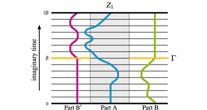
Figure 3: (Color online) Modified simulation cell used in DQMC simulations. Part $B$ appears twice as $B$ and $B^{\prime}$ and both extend from $0$ to $2\beta$ but its degrees of freedom only propagate in an interval of length $\beta$.

The replica scheme, as introduced above, has been formulated in the context of finite-temperature simulations with the inverse temperature $\beta$ entering as a natural parameter in the replica scheme. We now want to adopt this approach to the zero-temperature projective DQMC algorithm that aims at directly sampling the ground-state wavefunction (in lieu of the partition sum). As will become clear in the following, this adaptation will result in an algorithm that is much closer to the finite-temperature scheme introduced above than the original ground-state algorithm Sorella et al. (1989). At the heart of the ground-state algorithm is a projective scheme applied to a trial wave function $\left|\psi_{T}\right>$

$$\left|\psi\right>=\lim\limits_{\theta\rightarrow\infty}e^{-\theta\mathcal{H}}\left|\psi_{T}\right>\,,$$ (21)

which for sufficiently long projection times $\Theta$ yields the desired ground-state wavefunction $\left|\psi\right>$. The only requirement imposed on the trial wave function is for it to have a non-zero overlap with the actual ground-state wavefunction, in which case the projection will eliminate all contributions from excited states and converge to the ground-state wavefunction in the limit of $\theta\rightarrow\infty$. Again, we can introduce a normalization constant – similar to the normalization of the density matrix in the discussion preceding Eq. (16) above, which can again be written as a trace over the ground state density matrix

$$\mathcal{N}=\left<\psi|\psi\right>=\sum\limits_{\left|\mathcal{A}\right>}\left<\psi|\mathcal{A}\right>\left<\mathcal{A}|\psi\right>=\text{Tr}\,\left(\left|\psi\right>\left<\psi\right|\right)\,.$$ (22)

We can readily insert this normalization constant (or trace) into the denominator of the definition of the Rényi entropy in Eq. (18). Inserting the projection (21) into the nominator of the definition of the Rényi entropy in (18), we find an expression for the $\text{Tr}\,\rho_{A}^{\prime\,2}$ that looks very similar to the finite temperature expression discussed above

$$\text{Tr}\,\,\rho_{A}^{\prime\,2}=\lim\limits_{\theta\rightarrow\infty}\sum\limits_{\mathcal{A},\mathcal{A}^{\prime},\mathcal{B},\mathcal{B}^{\prime}}\left<\mathcal{A}{\mathcal{B}^{\prime}}\right|\exp\left({-\theta\mathcal{H}}\right)\left\lvert{\psi_{T}}\middle\rangle\!\middle\langle{\psi_{T}}\right\rvert\exp\left({-\theta\mathcal{H}}\right)\left|\mathcal{A}^{\prime}{\mathcal{B}^{\prime}}\right>\left<\mathcal{A}^{\prime}{\mathcal{B}}\right|\exp\left({-\theta\mathcal{H}}\right)\left\lvert{\psi_{T}}\middle\rangle\!\middle\langle{\psi_{T}}\right\rvert\exp\left({-\theta\mathcal{H}}\right)\left|\mathcal{A}\mathcal{B}\right>\,,$$ (23)

At first look, the only difference appears to be the occurrence of the density matrices $\left\lvert{\psi_{T}}\middle\rangle\!\middle\langle{\psi_{T}}\right\rvert$. However, note that the finite temperature algorithm works in a grand-canonical ensemble, while the trace above is given in a canonical ensemble. Nevertheless, we may safely adopt all of the machinery to implement the replica scheme described above, since the density matrices act as projectors onto the correct particle sectors.

IV Numerical stabilization

With the conceptual framework for the computation of Rényi entropies in DQMC simulations laid out in Secs. II and III above, we now turn to the technical aspects of its implementation. In particular, we discuss the numerical stabilization procedures enabling us to compute expectation values for these entanglement entropies for similar system sizes as for conventional observables (such as correlation functions) using the ordinary DQMC approach.

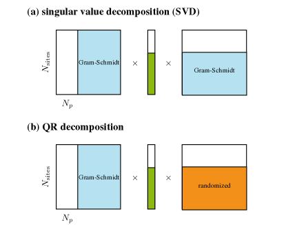
Figure 4: (Color online) Inversion scheme as applicable to SVD (top) and QR (bottom) based Green’s function calculations. Shown here is the example of the projected trial density matrix $B(\tau,\tau/2)\left|\psi_{T}\right>\left<\psi_{T}\right|B(\tau/2,0)$. Matrices with orthogonal columns or rows that form an incomplete basis are extended to a full basis using a Gram-Schmidt process, denoted here in blue. The singular value vectors are extended by a vector of decreasing numbers clearly separated from the smallest physical singular value by the singular value gap $\Delta$ here pictured in green. For the case of the QR decomposition matrices without orthogonal columns or rows appear naturally which are extended by a random matrix to match dimensions and ensure invertibility (for example by LU decomposition), pictured in orange.

IV.1 Invertibility of the matrix products

A fundamental problem in the adoption of the finite-temperature algorithm for ground-state properties is that the density matrix typically turns out to be singular, i.e. it is in general not invertible. As a consequence, the entire matrix product $\mathcal{B}(\tau)$ and its decomposed form (11) are also no longer invertible, which ultimately prevents to compute the equal-time Green’s function and the associated Monte Carlo weights. However, one can overcome this algebraic obstacle by numerically constructing a matrix that is equal to the matrix product $\mathcal{B}(\tau)$ up to machine precision, but whose matrix decomposition still yields invertible matrices as discussed in the following.

To see that the density matrix is in general a singular, non-invertible matrix let us consider a scenario where $N_{p}$ particles populate a lattice of $N$ sites. A trial wave function for such a scenario is typically constructed by diagonalizing the quadratic part of the Hamiltonian and then keeping only as many eigenvectors as the number of particles $N_{p}$ in the system Foo . This test wave function is thus represented as a matrix $\psi_{T}$ of dimension $N\times N_{p}$ with orthogonal columns, whereas the associated density matrix $\rho$ of size $N\times N$ is constructed as $\rho=\psi_{T}\psi_{T}^{\dagger}$. From this construction it becomes apparent that the density matrix must be rank deficient (since it is the product of two non-square matrices) and as such singular.

To elude this problem, we modify the matrices $U,D$, and $T$ of the singular value decomposition (12) such that they become invertible but leave the original matrix unchanged (up to machine precision, which we denote by $\varepsilon$). In Fig. 4, we illustrate how to do this in practice: Any non-square matrix with orthogonal (unitary) columns (or rows) can be extended to a square, fully orthogonal (unitary) matrix by applying a Gram-Schmidt process. To ensure that the original matrix, i.e. the one that results from remultiplying $U\,D\,T$, remains unchanged, we extend the diagonal matrix by values that are at least $1/\varepsilon$ smaller in magnitude than the smallest singular value found in the original $D$ matrix. Numerically, this means that none of the additional columns or rows actually contribute, because they are weighted below numerical precision by the diagonal matrix. If we multiply the modified matrices $U\times D\times T$, we recover the original, singular square matrix $B$.

IV.2 Stable calculation of the Green’s function

We now turn to the stable calculation of the equal-time Green’s function, which is calculated from the inverse of the matrix product $\mathcal{B}(\tau)$, see Eq. (11), and therefore also sensitively depends on the matrix decomposition discussed in the previous section. Despite having circumvented the problem of singularity, the calculation of the Green’s functions remains difficult, because the matrices of the decomposition typically remain ill-conditioned, i.e. they retain an extremely broad singular value spectrum resulting in a high condition number. The problem of calculating the Green’s function from ill-conditioned matrices in the finite-temperature algorithm has long been known and was solved by Hirsch and Fye Fye and Hirsch (1988) by using multiple consecutive matrix decompositions (instead of just one as given in Eq. (11)). These multiple decompositions can be arranged in an enlarged matrix of size $(N_{\text{sites}}\cdot N_{\text{decompositions}})\times(N_{\text{sites}}\cdot N_{\text{decompositions}})$, such that the determinant of this enlarged matrix remains equal to that of the original one, but the equal-time Green’s function can now be read off as a submatrix of the inverse of the enlarged matrix. The deeper reason that this approach allows to avoid the ill-conditioned matrix problem above is found in a considerably narrower singular value spectrum of the enlarged matrix. A maximum matrix size for the enlarged matrix is reached when each of the slice matrices is used as an input decomposition, i.e. $N_{\text{decompositions}}=N_{\tau}$. However, it is prohibitively expensive to invert such a large matrix. Fortunately, for our entanglement computations at hand it typically suffices to choose just two or three consecutive decompositions for the calculation of $G_{0}$ (for a simulation cell with a complete cut) and up to five for $G_{1}$ (for a simulation cell with a partial cut).

One more technical caveat in the entanglement computation that warrants attention arises when inserting the density matrices $\left\lvert{\psi_{T}}\middle\rangle\!\middle\langle{\psi_{T}}\right\rvert$ in the calculation of the trace over the reduced density matrix in Eq. (23). Upon building a matrix product like $\mathcal{B}=B(\theta,\theta/2)\left\lvert{\psi_{t}}\middle\rangle\!\middle\langle{\psi_{t}}\right\rvert B(\theta/2,0)$ we start from the right and multiply slice matrices $\textsf{{B}}(i)$, applying the stabilization procedure using successive matrix decompositions, until we built up the decomposition for the slice matrix group $B(\theta/2,0)$. Up until this point in imaginary time, these matrices are square and invertible but now the insertion of the singular density matrix turns the entire product into a singular matrix. If we now carried on multiplying slice matrices on the left and decomposing the resulting matrices as we had done before, we would expect to find $N_{p}$ non-zero singular values, corresponding to the particle number of the trial wave function and $N-N_{p}$ zero singular values. In practice, however, a decomposition algorithm like SVD or QR will typically find only the $N_{p}$ non-zero singular values to high precision but the $N-N_{p}$ remaining singular values (strictly zero in theory) are found to be zero only relative to the actual non-zero singular values. These inaccuracies will accumulate as we keep multiplying more slice groups and decomposing the resulting matrix products which ultimately results in incorrect Green’s matrices.

This problem can be overcome by a modification of the stack structure, whose implementation we discuss in the following for the case of calculating $G_{0}$. In this modified stack structure, we keep track of three such stacks: one which is built from the bra version of the wave function and includes decompositions obtained from matrices of the form $\left<\psi\right|B(\tau,\tau^{\prime})$, a second one which is simply the ket version based on $B(\tau,\tau^{\prime})\left|\psi\right>$ and finally a third one that is used as temporary storage and includes decompositions of the full slice matrix groups $B(\tau,\tau^{\prime})$. In combination, these three stacks allow to calculate $G_{0}$ for a given imaginary time slice (at imaginary time $n\cdot\Delta$, see section II.2). An example configuration of the three stacks for imaginary time $\tau=n\cdot\Delta$ looks as follows

These three stacks can be used to set up a $3\cdot N_{\text{sites}}\times 3\cdot N_{\text{sites}}$ matrix and to subsequently calculate the Green’s function and the corresponding Monte Carlo weight. Alternatively, if the condition numbers of the matrices allow it, it is possible to contract two or even all of them for a faster calculation. In that case, one has to think about the order of the matrix contractions. Naturally, the optimal choice is the one that keeps the condition numbers for the resulting matrices as small as possible, thus ensuring the highest stability of the following operations. Note that the number of contractions can vary for each recalculation and should be chosen according to the magnitude of the relative error between propagated and recalculated Green’s function as defined in Eq. (14).

These numerical refinements are incorporated in the modified flow diagram of our DQMC algorithm in Fig. 5.

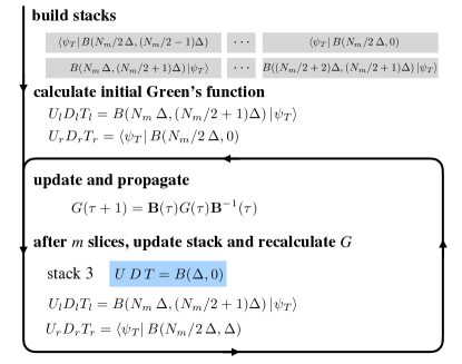
Figure 5: (Color online) Flow diagram of the modified DQMC algorithm for the simulation of the partition function $Z_{0}$ with complete cut in imaginary time. Stacks are initialized starting from the bra and ket version of the wave function and subsequently used to calculate an initial Green’s function. This Green’s function is then used to update the auxiliary field time slice by time slice and recalculated after $m$ time steps to retain numerical stability. Intermediate decompositions of slice matrix groups $U,D,T$ without wave function are stored in a third stack, depicted in blue.

As for the calculation of $G_{1}$, we have to keep track of five individual stacks but the rest of the algorithm works exactly as just described for $G_{0}$.

IV.3 Choice of Hubbard-Stratonovich transformation

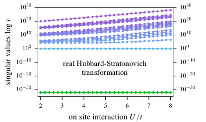
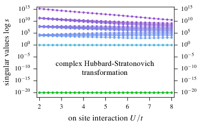
Figure 6: (Color online) The singular value spectrum of the matrix $B(\Theta/2,0)\left|\psi_{T}\right>$ i.e. the projected wave function, on a logarithmic scale for a real (left) and complex (right) Hubbard-Stratonovich transformation. The projection time is $\theta=10$.

At the heart of the DQMC approach is the decoupling of quartic terms in the Hamiltonian using a Hubbard-Stratonovich transformation. In general, there is a multitude of possible alternatives to perform this transformation. Depending on the physics of interest, common choices include a decoupling in the spin or charge channels which leads to either a real or complex Hubbard-Stratonovich transformation that preserves or breaks SU(2) symmetry, respectively. From an algorithmic point of view, the choice of Hubbard-Stratonovich transformation can greatly affect the numerical stability and convergence of the DQMC approach.

To illustrate the influence of the choice of Hubbard-Stratonovich transformation on the algorithmic performance, let us consider the example of a density-density interaction of the general form

$$\hat{U}_{\alpha\beta}=U_{\alpha\beta}\,n_{\alpha}n_{\beta}\,,$$ (24)

where the indices $\alpha$ and $\beta$ may represent adjacent sites for a nearest-neighbor interaction or different spin species for a given site. In either case, we are looking to identify a quadratic operator $A$ such that we can apply the Hubbard-Stratonovich transformation

$$e^{\frac{1}{2}A^{2}}=\sqrt{2\pi}\int\limits_{-\infty}^{\infty}\textrm{d}s\;e^{-\frac{1}{2}s^{2}-s\,A}\,,$$ (25)

where $s$ is the auxiliary field introduced in the decoupling scheme. To do so, we will rewrite the interaction term (24) in an appropriate form. There are two possible choices

$$n_{\alpha}n_{\beta} =-\dfrac{1}{2}(n_{\alpha}-n_{\beta})^{2}+\dfrac{1}{2}(n_{\alpha}^{2}+n_{\beta}^{2})\,,$$ (26)

$$n_{\alpha}n_{\beta} =\dfrac{1}{2}(n_{\alpha}+n_{\beta})^{2}-\dfrac{1}{2}(n_{\alpha}^{2}+n_{\beta}^{2})\,,$$ (27)

with the quadratic operator corresponding to the first term, i.e. $A=(n_{\alpha}-n_{\beta})^{2}$ or $A=(n_{\alpha}+n_{\beta})^{2}$, respectively. For the scenario of a spin-spin onsite-interaction the first choice of $A$ in Eq. (26) corresponds to the squared magnetization and thus a decoupling in the spin channel. For the second choice (27) the operator $A$ corresponds to the squared total charge and thus corresponds to a decoupling in the charge channel.

Note that in order to perform the Hubbard-Stratonovich transformation (25), the auxiliary field $s$ does not necessarily have to be continuous, as probably suggested by the integral form of Eq. (25). For some cases, it suffices to work with a discrete field that is constrained to, e.g., take values $\pm 1$ such as the case of the spinful Hubbard model, with most applications typically needing no more than a four-valued discrete field Assaad et al. (1997).

Applying the Hubbard-Stratonovich transformation (25) after bringing the operators into squared form (26, 27) gives the following expressions

$$e^{-\Delta\tau Un_{\alpha}n_{\beta}}=\dfrac{1}{2}\sum\limits_{s=\pm 1}\prod\limits_{a=\alpha,\beta}e^{-\left(s\lambda+\frac{U\Delta\tau}{2}\right)n_{a}}$$ (28)

and

$$e^{-\Delta\tau Un_{\alpha}n_{\beta}}=\dfrac{1}{2}\sum\limits_{s=\pm 1}\prod\limits_{a=\alpha,\beta}e^{-\left(s\lambda+\frac{U\Delta\tau}{2}\right)\left(n_{a}-\frac{1}{2}\right)}\,,$$ (29)

respectively. Here the constant $\lambda$ is given by

$$\cosh{\left(\lambda\right)}=e^{\frac{1}{2}U\Delta\tau}$$ (30)

and

$$\cosh{\left(\lambda\right)}=e^{-\frac{1}{2}U\Delta\tau}\,,$$ (31)

respectively. Note that Eqs. (30,31) imply that depending on the sign of the interaction $U$, the constant $\lambda$ can either be real or complex valued.

At first look, one might think that the real-valued Hubbard-Stratonovich transformation leads to lower computational cost. However, in computations of the entanglement entropy it is the complex-valued Hubbard-Stratonovich transformation that should be used preferably. The reason for this preference is that the type of Hubbard-Stratonovich transformation also greatly affects the singular value spectrum of the matrix decompositions discussed in the previous subsection. To illustrate this point, we show in Fig. 6 a comparison of the singular value spectrum of the matrix $B(\Theta/2,0)\left|\psi_{T}\right>$, i.e. the projected wave function, obtained for real and complex Hubbard-Stratonovich transformations. The data is calculated for a bilayer Hubbard model on a square lattice of size $4\times 4\times 2$ at half filling and equal hopping within and between the layers, i.e. $t=t^{\prime}$, but varying onsite interaction $U$, see also Sec. V for a more detailed discussion of this model. In the complex case, the range of the singular values is seen to decrease as the interaction increases, hence reducing the condition number and stabilizing the algorithm. In the real case, the behavior is found to be exactly opposite with the condition number becoming worse as the interaction strength increases.

As a consequence, we always use complex-valued Hubbard-Stratonovich transformation in the computation of Rényi entanglement entropies.

IV.4 Convergence

One key distinction of our zero-temperature entanglement calculations in the projective DQMC approach outlined in this manuscript and the closely related finite-temperature algorithm is in the type of simulated ensemble. While the finite-temperature algorithm is sampling states from a grand canonical ensemble, the projective scheme samples a canonical ensemble of fixed particle number (encoded in the trial wave function). This seemingly small modification of the ensemble is found to have some rather noticeable impact on the convergence properties of the projective algorithm. To ensure convergence, we resort to a technical trick by introducing an artificial chemical potential in the Hamiltonian

$$H^{\prime}=H+\mu_{a}\sum\limits_{i}n_{i}\,.$$ (32)

Note that the inclusion of this artificial chemical potential $\mu_{a}$ is not altering the physics of the original problem, since we keep working in a canonical ensemble with a fixed particle number. To understand why it is nevertheless beneficial to include this term, let us first note that, on a technical level, such a term is represented by a diagonal matrix that has the ability to significantly shift the singular value spectrum. This is displayed in Fig. 7, which plots the smallest singular value of the unmodified matrix $B(\Theta/2,0)\left|\psi\right>$.

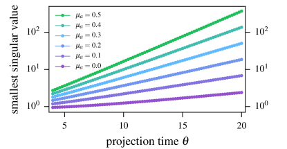
Figure 7: (Color online) Evolution of the smallest singular value with projection time $\Theta$ for various values for the artificial chemical potential $\mu_{a}$.

Clearly visible is the increase of the magnitude of the smallest singular value with increasing projection time $\Theta$ and increasing chemical potential $\mu_{a}$. If we now consider the convergence of the entanglement entropy upon inclusion of this artificial chemical potential term, we find that already a small additional potential dramatically improves the convergence of the entanglement entropy as a function of projection time as shown in Fig. 8. Further increasing the artificial chemical potential we find that the convergence eventually saturates, in the case at hand for about $\mu_{a}\approx 0.4$. In general, the optimal value of $\mu_{a}$ depends rather sensitively on the parameters of the Hamiltonian and needs to be chosen with great care.

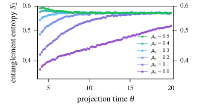
Figure 8: (Color online) Convergence of the Rényi entanglement entropy $S_{2}$ in the projective DQMC algorithm versus projection time for varying values of the artificial chemical potential $\mu_{a}$. The Rényi entropy is calculated for a half-filled Hubbard model on the square lattice for $U/t=4$ with an equal-size bipartition of the lattice.

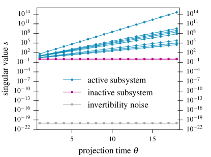
Figure 9: (Color online) Magnitude of the singular values of the Green’s function in the replicated system for a Hubbard model on a square lattice at half filling, an on site interaction of $U/t=4$ and $\mu_{a}=0.5$.

Closer inspection of the convergence properties of our entanglement DQMC algorithm reveals that the added chemical potential (32) only affects the calculation of the Green’s function $G_{1}$ associated with the partition sum $Z_{1}$, i.e. the partition sum for the partially cut system, see Fig. 2. This observation already hints at the origin of the improved convergence. For the partition sum $Z_{1}$ all slice matrices are obtained from the “unfolded” Hamiltonian (20), where we fold out subsystem $B$ as illustrated in Fig. 3. The slice matrices include blocks of identity and zero matrices to accommodate the currently “inactive” subsystem $B$ or $B^{\prime}$, i.e. the one which is deactivated by the $\Theta$-function in the Hamiltonian (20). As demonstrated in Fig. 9 this greatly affects the singular value spectrum by introducing $N_{B}$ singular values of unit value (indicated by the magenta data set) representing the said subsystem. Comparing Figs. 7 and 9, we observe that once the difference between the smallest singular value of the the active subsystem becomes separated from the unit singular values corresponding to the inactive subsystem, the simulation has a chance to converge. Thus, the requirement is that this gap $\Delta_{s}$ in the singular value spectrum has to be sufficiently large. In our studies we empirically find that $\Delta_{s}\approx 10^{2}$ turns out to be a good choice for all calculations.

V Application to the bilayer Hubbard model

We round off the technical discussion of this manuscript with one example illustrating the application of entanglement computations to identify quantum phases of interacting many-fermion systems. We resort to the bilayer Hubbard model – a paradigmatic model that allows to study the transition between a Mott insulator and a band insulator. Whether these two insulating states are fundamentally distinct or can in general be adiabatically connected into one another Anfuso and Rosch (2007), has been a question of debate Essler and Tsvelik (2002, 2005); Fuhrmann et al. (2006); Konik et al. (2006); Berthod et al. (2006); Garg et al. (2006); Stanescu et al. (2007); Rosch (2007); Kancharla and Okamoto (2007a); Paris et al. (2007); Kancharla and Dagotto (2007). This discussion mostly preceded the days of the topological insulator Hasan and Kane (2010); Qi and Zhang (2011) – a second type of band insulator that can be clearly distinguished from the conventional “trivial” band insulator by certain topological invariants Kane and Mele (2005a, b), while its fundamental distinction to correlated Mott insulators (possibly exhibiting topological order as well) is an open question of much current interest Wang et al. (2014b).

Here we want to apply an entanglement perspective on the elementary phase diagram of the bilayer Hubbard model

$$H=-t\sum\limits_{\langle i,j\rangle,\sigma}c^{\dagger}_{i,\sigma}c_{j,\sigma}-t^{\prime}\sum\limits_{\langle i,j\rangle^{\prime},\sigma}c^{\dagger}_{i,\sigma}c_{j,\sigma}+U\sum\limits_{i}n_{i,\uparrow}n_{j,\downarrow}\,,$$ (33)

which at its core describes the competition between conventional (free-fermion) band structures arising from hopping within and between the layer of a double-layer square lattice (parametrized by hopping amplitudes $t$ and $t^{\prime}$, respectively) and Mott physics arising from an on-site Coulomb repulsion $U$. A schematic phase diagram for this model in terms of the on-site interaction $U$ and the interlayer hopping $t^{\prime}$ is given in Fig. 10. For sufficiently large interlayer hopping strength $t^{\prime}$ and any value of $U$ the system is a featureless band insulator, while for sufficiently large $U$ and small interlayer hopping $t^{\prime}$ the system forms a Mott insulator with antiferromagnetic order. The phase transition from Mott to band insulator has been studied using a variety of methods in the past Weihong (1997); Wang et al. (2006); Kancharla and Okamoto (2007b); Bouadim et al. (2008); Hamer et al. (2012); Helmes and Wessel (2014); Rüger et al. (2014); Chang et al. (2014); Golor et al. (2014). In the absence of a Hubbard interaction $U$ and small interlayer hopping we have a metal. Whether this metallic state survives for small Hubbard $U$ (and small interlayer hopping $t^{\prime}$ ) or immediately gives way to Mott physics is still under debate, with dynamical mean field theory (DMFT) Kancharla and Okamoto (2007a) and DQMC simulations Chang et al. (2014) pointing to an extended metallic phase, while a functional renormalization group (FRG) analysis Golor et al. (2014) finds an immediate breakdown of the metallic phase upon inclusion of the Hubbard term.

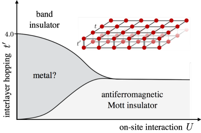
Figure 10: (Color online) Schematic phase diagram for the bilayer Hubbard model at half filling, adapted from dynamical mean field theory (DMFT) Kancharla and Okamoto (2007a), DQMC simulations Chang et al. (2014), and functional renormalization group (FRG) calculations Golor et al. (2014). It comprises two insulating phases, a band insulator for sufficiently strong interlayer hopping $t^{\prime}\gtrsim 4$, an antiferromagnetic insulator for weak interlayer hopping strength and large on-site Coulomb repulsion $U$. There possibly is an extended metallic phase in the regime of small Coulomb repulsion and interlayer hopping as indicated in the phase diagram, with DMFT and DQMC simulations in favor of it Kancharla and Okamoto (2007a); Chang et al. (2014), while FRG calculations point to an absence of a metallic phase for any finite Coulomb repulsion Golor et al. (2014). The inset depicts of the bilayer lattice. The intralayer hoppings are indicated by $t$, while $t^{\prime}$ denotes the interlayer hoppings.

Our DQMC approach is ideally suited to compute Rényi entanglement entropies over a wide range of parameters, in particular going deep into the regime of strong coupling $U>t,t^{\prime}$. To do so, we consider a bipartition of the system into a strip of width $L/4\times L\times 2$ and its complement. For this type of cut, which includes both the upper and lower layer, we expect that the entanglement signature of the band insulator is rather trivial – with the formation of singlet dimers on the rungs between the layers any cut between the rungs will effectively see no significant entanglement contribution, similar to the entanglement signature of an unentangled product state. Deep in the Mott regime we expect to observe the prevalent entanglement signature of any entangled quantum many-body state – a finite entanglement entropy that is subject to the famous boundary-law scaling Eisert et al. (2010). For any metallic state we expect to observe an even stronger entanglement signature in the form of a logairthmic violation of the aforementioned boundary law Wolf (2006); Gioev and Klich (2006).

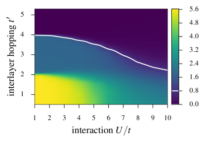
Figure 11: (Color online) Color-coded Rényi entanglement entropy $S_{2}$ for the bilayer Hubbard model calculated for a bipartition of a $4\times 4\times 2$ system (with the system divided into a strip of extent $1\times 4\times 2$ and its complement). The different entanglement regimes clearly reveal the general characteristics of the underlying phase diagram. For dominant interlayer coupling $t^{\prime}\gtrsim 4$ the vanishingly small entanglement points to the featureless band insulator with singlet formation on the interlayer rungs. For moderate interlayer coupling, the finite entanglement reveals the Mott insulator. For small interlayer coupling and small onsite interaction, a third entanglement regime can be distinguished (indicated by the yellow region), which possibly points to an additional metallic phase. The phase boundary separating the band insulator is indicated by an equipotential line of $S_{2}=0.8$. The relevant color values corresponding to these values of the entanglement entropy are also marked on the colorbar by white lines.

As a first step we have scanned the absolute value of the Rényi entropy for $t^{\prime}\in\left[0.5,5.0\right]$ as illustrated in Fig. 11 for a system of $4\times 4\times 2$ sites. Clearly, several distinct regimes of almost constant amount of entanglement can be readily distinguished thereby revealing some of the core features of the phase diagram. For instance, one can clearly identify a regime of almost vanishing entanglement for large interlayer coupling $t^{\prime}$ – this is the band insulator as argued above. The finite entanglement clearly present in the lower part of the phase diagram points to at least one separate regime, possibly two when considering the step-like enhancement of the Rényi entropy for $t^{\prime}/t<2$ and $U/t\lesssim 4$ indicated by the yellow color. The Rényi entropy along a vertical cut through the data of Fig. 11 is shown in Fig. 12 for $U/t=4$.

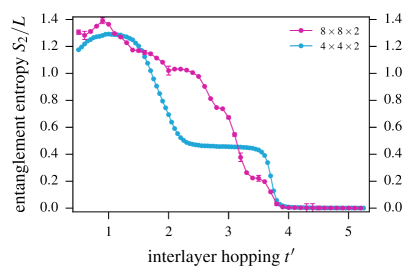
Figure 12: (Color online) Rényi entanglement entropy $S_{2}$ for the bilayer Hubbard model along a vertical cut through the phase diagram of Fig. 11 at $U/t=4$. Data for different system sizes is shown.

To further substantiate the nature of the phase(s) in the lower half of the phase diagram we consider the scaling of the Rényi entropy with system size. In Fig. 13 we show results for the Rényi entropy for different values of the onsite Coulomb repulsion $U/t=2,4,8$ and $16$ and fixed interlayer hopping $t^{\prime}/t=1$. With the entropy renormalized by the linear system size $L$, the boundary law scaling expected for the Mott insulator corresponds to a flat line. This is precisely what we find for moderate to large Hubbard interaction $U/t=4,8,16$. In contrast, for small Hubbard interaction $U/t=2$ the clearly noticeable slope of the data points suggests an additional logarithmic contribution to the entanglement entropy. Precisely such an $S\propto L\log L$ scaling is expected for a two-dimensional metal with a Fermi surface Wolf (2006); Gioev and Klich (2006). Note, however, that we are looking at rather small system sizes when inferring this logarithmic contribution and it would be highly desirable to go to substantially larger system sizes to exclude possible finite-size effects. Unfortunately, such a substantial increase in system sizes does not seem feasible with the current algorithms and state-of-the-art computational resources. Nevertheless, with the data at hand the entanglement point of view is certainly adding support to a scenario, in which the metallic state survives the inclusion of a moderately small Hubbard interaction.

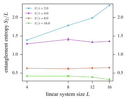
Figure 13: (Color online) Finite-size scaling of the entanglement entropy $S_{2}$ renormalized by the linear system size $L$ for the bilayer Hubbard model at different values of the on-site interaction $U/t$ and fixed interlayer coupling $t^{\prime}/t=1$. Note the logarithmic scale of the abscissa.

VI Summary

To summarize, we have laid out a number of algorithmic advances to overcome the numerical instabilities of computing entanglement entropies for interacting many-fermion systems within the DQMC framework. The basic algorithm Broecker and Trebst (2014) is an adaptation of the replica scheme to the DQMC approach, which on a technical level converts the finite-temperature algorithm (in the grand-canonical ensemble) to a ground-state projective algorithm (in the canonical ensemble). Our numerical improvements of this approach, reported on here, include (i) a numerical stabilization of the matrix inversion of seemingly singular matrix products via a refined matrix decomposition, (ii) a numerical stabilization of the calculation of the Green’s function using this refined matrix decomposition, (iii) an optimal choice of Hubbard-Stratonovich transformation, which typically turns out to be a complex-valued one, and (iv) the inclusion of an artificial chemical potential to significantly improve the convergence of the algorithm. With these algorithmic enhancements implemented, we find that one can reach similar system sizes as for the calculation of more conventional observables in the original projective DQMC scheme and showcased the algorithm by applying it to the bilayer Hubbard model.

Form a physics point of view, probably the most interesting application of the computational scheme at hand is to showcase that one can positively identify the formation of macroscopic entanglement in an interacting many-fermion system exhibiting a phase with intrinsic topological order such as the recently proposed models of Dirac fermions coupled to a Z₂ gauge field Assaad and Grover ; Gazit et al. . This is ongoing work.