A spectral algorithm for fast de novo layout of uncorrected long nanopore reads

Abstract

1 Motivation:

New long read sequencers promise to transform sequencing and genome assembly by producing reads tens of kilobases long. However, their high error rate significantly complicates assembly and requires expensive correction steps to layout the reads using standard assembly engines.

2 Results:

We present an original and efficient spectral algorithm to layout the uncorrected nanopore reads, and its seamless integration into a straightforward overlap/layout/consensus (OLC) assembly scheme. The method is shown to assemble Oxford Nanopore reads from several bacterial genomes into good quality ($\sim$99% identity to the reference) genome-sized contigs, while yielding more fragmented assemblies from the eukaryotic microbe Sacharomyces cerevisiae.

3 Availability and implementation:

https://github.com/antrec/spectrassembler

4 Contact:

antoine.recanati@inria.fr

5 Introduction

De novo whole genome sequencing seeks to reconstruct an entire genome from randomly sampled sub-fragments whose order and orientation within the genome are unknown. The genome is oversampled so that all parts are covered multiple times with high probability.

High-throughput sequencing technologies such as Illumina substantially reduce sequencing cost at the expense of read length, which is typically a few hundred base pairs long (bp) at best. Yet, de novo assembly is challenged by short reads, as genomes contain repeated sequences resulting in layout degeneracies when read length is shorter or of the same order than repeat length [Pop,, 2004].

Recent long read sequencing technologies such as PacBio’s SMRT and Oxford Nanopore Technology (ONT) have spurred a renaissance in de novo assembly as they produce reads over 10kbp long [Koren and Phillippy,, 2015]. However, their high error rate ($\sim$15%) makes the task of assembly difficult, requiring complex and computationally intensive pipelines.

Most approaches for long read assembly address this problem by correcting the reads prior to performing the assembly, while a few others integrate the correction with the overlap detection phase, as in the latest version of the Canu pipeline [Koren et al.,, 2016] (former Celera Assembler [Myers et al.,, 2000]).

Hybrid techniques combine short and long read technologies: the accurate short reads are mapped onto the long reads, enabling a consensus sequence to be derived for each long read and thus providing low-error long reads (see for example Madoui et al., [2015]). This method was shown to successfully assemble prokaryotic and eukaryotic genomes with PacBio [Koren et al.,, 2012] and ONT [Goodwin et al.,, 2015] data. Hierarchical assembly follows the same mapping and consensus principle but resorts to long read data only, the rationale being that the consensus sequence derived from all erroneous long reads matching a given position of the genome should be accurate provided there is sufficient coverage and sequencing errors are reasonably randomly distributed: for a given base position on the genome, if 8 out of 50 reads are wrong, the majority vote still yields the correct base. Hierarchical methods map long reads against each other and derive, for each read, a consensus sequence based on all the reads that overlap it. Such an approach was implemented in HGAP [Chin et al.,, 2013] to assemble PacBio SMRT data, and more recently by Loman et al., [2015], to achieve complete de novo assembly of Escherichia coli with ONT data exclusively.

Recently, Li, [2016] showed that it is possible to efficiently perform de novo assembly of noisy long reads in only two steps, without any dedicated correction procedure: all-vs-all raw read mapping (with minimap) and assembly (with miniasm). The miniasm assembler is inspired by the Celera Assembler and produces unitigs through the construction of an assembly graph. Its main limitation is that it produces a draft whose error rate is of the same order as the raw reads.

Here, we present a new method for computing the layout of raw nanopore reads, resulting in a simple and computationally efficient protocol for assembly. It takes as input the all-vs-all overlap information (e.g. from minimap, MHAP [Berlin et al.,, 2015] or DALIGNER [Myers,, 2014]) and outputs a layout of the reads (i.e. their position and orientation in the genome). Like miniasm, we compute an assembly from the all-vs-all raw read mapping, but achieve improved quality through a coverage-based consensus generation process, as in nanocorrect [Loman et al.,, 2015], although reads are not corrected individually in our case.

The method relies on a simple spectral algorithm akin to Google’s PageRank [Page et al.,, 1999] with deep theoretical underpinnings, described in §6.1. It has successfully been applied to consecutive-ones problems arising in physical mapping of genomes [Atkins and Middendorf,, 1996], ancestral genome reconstructions [Jones et al.,, 2012], or the locus ordering problem [Cheema et al.,, 2010], but to our knowledge has not been applied to de novo assembly problems. In §6.2, we describe an assembler based on this layout method, to which we add a consensus generation step based on POA [Lee et al.,, 2002], a multi-sequence alignment engine. Finally, we evaluate this pipeline on prokaryotic and eukaryotic genomes in §7, and discuss possible improvements and limitations in §8.

6 Methods

6.1 Layout computation

We lay out the reads in two steps. We first sort them by position, i.e., find a permutation $\pi$ such that read $\pi(1)$ will be positioned before read $\pi(2)$ on the genome. Then, we iteratively assign an exact position (i.e., leftmost basepair coordinate on the genome) to each read by using the previous read’s position and the overlap information.

The key step is the first one, which we cast as a seriation problem, i.e. we seek to reconstruct a linear order between $n$ elements using unsorted, pairwise similarity information [Atkins et al.,, 1998; Fogel et al.,, 2013]. Here the $n$ elements are the reads, and the similarity information comes from the overlapper (e.g. from minimap).

The seriation problem is formulated as follows. Given a pairwise similarity matrix $A_{ij}$, and assuming the data has a serial structure, i.e. that there exists an order $\pi$ such that $A_{\pi(i)\pi(j)}$ decreases with $|i-j|$, seriation seeks to recover this ordering $\pi$ (see Figure 1 for an illustration). If such an order $\pi$ exists, it minimizes the 2-SUM score,

$$\text{2-SUM}(\pi)=\sum_{i,j=1}^{n}A_{ij}\left(\pi(i)-\pi(j)\right)^{2},$$ (1)

and the seriation problem can be solved as a minimization over the set of permutation vectors [Fogel et al.,, 2013]. In other words, the permutation $\pi$ should be such that if $A_{ij}$ is high (meaning that $i$ and $j$ have a high similarity), then $\left(\pi(i)-\pi(j)\right)^{2}$ should be low, meaning that the positions $\pi(i)$ and $\pi(j)$ should be close to each other. Conversely, if $A_{ij}=0$, the positions of $i$ and $j$ in the new order may be far away without affecting the score.

When using seriation to solve genome assembly problems, the similarity $A_{ij}$ measures the overlap between reads $i$ and $j$. In an ideal setting with constant read length and no repeated regions, two overlapping reads should have nearby positions on the genome. We therefore expect the order found by seriation to roughly match the sorting of the positions of the reads.

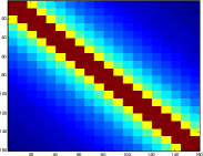
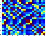
Figure 1: A similarity matrix reordered with the spectral algorithm. The original matrix (left) has values that decrease when moving away from the diagonal (red : high value, blue : low value). It is randomly permuted (right), and the spectral algorithm will find back the original ordering.

The problem of finding a permutation over $n$ elements is combinatorial. Still, provided the original data has a serial structure, an exact solution to seriation exists in the noiseless case [Atkins et al.,, 1998] using spectral clustering, and there exist several convex relaxations allowing explicit constraints on the solution [Fogel et al.,, 2013].

The exact solution is directly related to the well-known spectral clustering algorithm. Indeed, for any vector $\mathbf{x}$, the objective in (1) reads

$$\sum_{i,j=1}^{n}A_{ij}\left(x_{i}-x_{j}\right)^{2}=x^{T}L_{A}x,\quad L_{A}=\mathop{\bf diag}(A\mathbf{1})-A$$

where $L_{A}$ is the Laplacian matrix of $A$. This means that the 2-SUM problem amounts to

$$\min_{\pi}\pi^{T}L_{A}\pi$$

where $\pi$ is a permutation vector. Roughly speaking, the spectral clustering approach to seriation relaxes the constraint “$\pi$ is a permutation vector” into “$\pi$ is a vector of $\mathbb{R}^{n}$ orthogonal to the constant vector $\mathbf{1}=(1,...,1)^{T}$” with fixed norm. The problem then becomes

$$\min_{\{\mathbf{1}^{T}\pi=0,\,\|\pi\|_{2}=1\}}\pi^{T}L_{A}\pi$$

This relaxed problem is an eigenvector problem. Finding the minimum over normalized vectors $x$ yields the eigenvector associated to the smallest eigenvalue of $L_{A}$, but the smallest eigenvalue, $0$, is associated with the eigenvector $\mathbf{1}$, from which we cannot recover any permutation. However, if we restrict $x$ to be orthogonal to $\mathbf{1}$, the solution is the second smallest eigenvector, called the Fiedler vector. A permutation is recovered from this eigenvector by sorting its coefficients: given $\mathbf{x}=(x_{1},x_{2},...,x_{n})$, the algorithm outputs a permutation $\pi$ such that $x_{\pi(1)}\leq x_{\pi(2)}\leq...\leq x_{\pi(n)}$. This procedure is summarized as Algorithm 1.

In fact, [Atkins et al.,, 1998] showed that under the assumption that $A$ has a serial structure, Algorithm 1 solves the seriation problem exactly, i.e. recovers the order $\pi$ such that $A_{\pi(i)\pi(j)}$ decreases with $|i-j|$. This means that we solve the read ordering problem by simply solving an extremal eigenvalue problem, which has low complexity (comparable to Principal Component Analysis (PCA)) and is efficient in practice (see Supplementary Figure S1 and Table 9).

Algorithm 1 Spectral ordering

0:  Connected similarity matrix $A\in\mathbb{R}^{n\times n}$

1:  Compute Laplacian $L_{A}=\mathop{\bf diag}(A\mathbf{1})-A$

2:  Compute second smallest eigenvector of $L_{A}$, $\mathbf{x^{*}}$

3:  Sort the values of $\mathbf{x^{*}}$

3:  Permutation $\pi:\mathbf{x^{*}}_{\pi(1)}\leq\mathbf{x^{*}}_{\pi(2)}\leq...\leq\mathbf{x^{*}}_{\pi(n)}$

Once the reads are reordered, we can sequentially compute their exact positions (basepair coordinate of their left end on the genome) and orientation. We assign position 0 and strand “+” to the first read, and use the overlap information (position of the overlap on each read and mutual orientation) to compute the second read’s position and orientation, etc. More specifically, when computing the position and orientation of read $i$, we use the information from reads $i-1,...,i-c$ to average the result, where $c$ roughly equals the coverage, as this makes the layout more robust to misplaced reads. Note that overlappers relying on hashing, such as minimap and MHAP, do not generate alignments but still locate the overlaps on the reads, making this positioning step possible. Thanks to this “polishing” phase, we would still recover the layout if two neighboring reads were permuted due to consecutive entries of the sorted Fiedler vector being equal up to the eigenvector computation precision, for example.

6.2 Consensus generation

We built a simple assembler using this layout idea and tested its accuracy. It is partly inspired by the nanocorrect pipeline of Loman et al., [2015] in which reads are corrected using multiple alignments of all overlapping reads. These multiple alignments are performed with a Partial Order Aligner (POA) [Lee et al.,, 2002] multiple-sequence alignment engine. It computes a consensus sequence from the alignment of multiple sequences using a dynamic programming approach that is efficient when the sequences are similar (which is the case if we trim the sequences to align their overlapping parts). Specifically, we used SPOA, a Single Instruction Multiple Data implementation of POA developed in Vaser et al., [2016].

The key point is that we do not need to perform multiple alignment using all reads, since we already have a layout. Instead, we can generate a consensus sequence for, say, the first 3000 bp of the genome by aligning the parts of the reads that are included in this window with SPOA, and repeat this step for the reads included in the window comprising the next 3000 bp of the genome, etc. In practice, we take consecutive windows that overlap and then merge them to avoid errors at the edges, as shown in Figure 2. The top of the figure displays the layout of the reads broken down into three consecutive overlapping windows, with one consensus sequence generated per window with SPOA. The final assembly is obtained by iteratively merging the window $k$+1 to the consensus formed by the windows $1,\ldots,k$.

The computational complexity for aligning $N$ sequences of length $L$ with POA, with an average divergence between sequences $\epsilon$, is roughly $O(mNL^{2})$, with $m\simeq(1+2\epsilon)$. With $10\%$ of errors, $m$ is close to 1. If each window of size $L_{w}$ contains about $C$ sequences, the complexity of building the consensus in a window is $O(mCL_{w}^{2})$. We compute $L_{g}/L_{w}$ consensus windows, with $L_{g}$ the length of the genome (or contig), so the overall complexity of the consensus generation is $O(mCL_{g}L_{w})$. We therefore chose in practice a window size relatively small, but large enough to prevent mis-assemblies due to noise in the layout, $L_{w}=3$kbp.

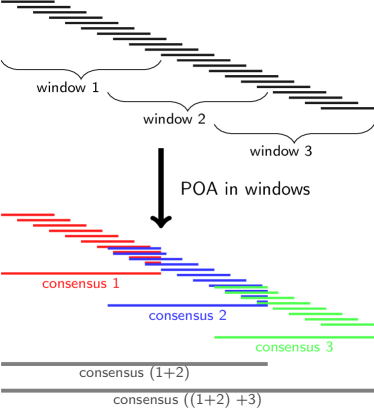
Figure 2: Consensus generation. Given the layout, the genome is sliced into overlapping windows, and a consensus is computed in each window. The final consensus is then obtained by merging the consensus windows.

6.3 Overlap-based similarity and repeats handling

In practice, we build the similarity matrix $A$ as follows. Given an overlap found between the i-th and j-th reads, we set $A_{ij}$ equal to the overlap score (or number of matches, given in tenth column of minimap or fourth column of MHAP output file). Such matrices are sparse: a read overlaps with only a few others (the number of neighbors of a read in the overlap graph roughly equals the coverage). There is no sparsity requirement for the algorithm to work, however sparsity lowers RAM usage since we store the $n\times n$ similarity matrix with about $n\times C$ non-zero values, with $C$ the coverage. In such cases, the ordered similarity matrix is band diagonal.

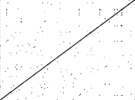
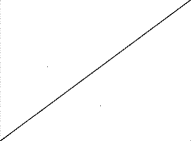
Figure 3: Similarity matrix for E. coli ONT sequences before (left) and after (right) thresholding. The positions of the reads were obtained by mapping to the reference genome with GraphMap [Sović et al.,, 2016].

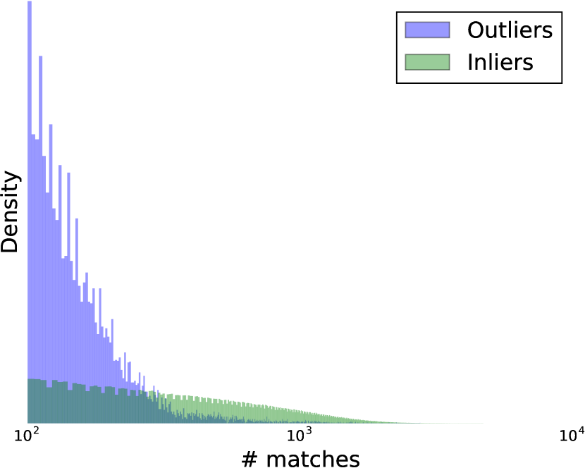
(a) A. baylyi ONT

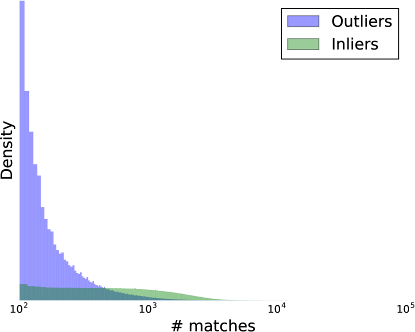
(b) S. cerevisiae ONT R7.3

(c) S. cerevisiae ONT R9

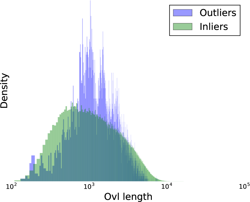
(d) A. baylyi ONT

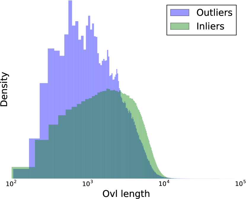
(e) S. cerevisiae ONT R7.3

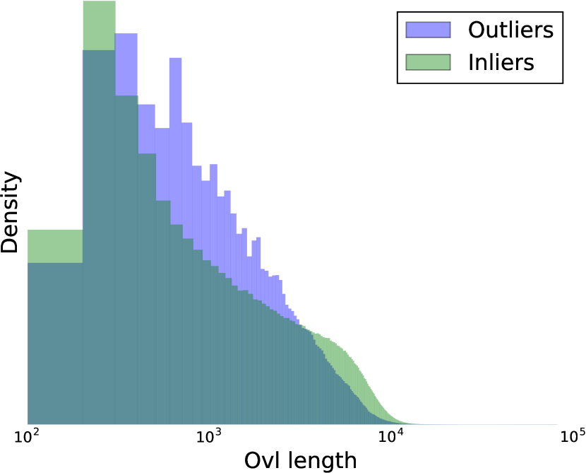
(f) S. cerevisiae ONT R9

Figure S2: Histograms of overlap scores [number of matches from minimap] (a-c) and overlap lengths (d-f) for the ONT datasets, for outliers (blue) and inliers (green). The x-axis is in log scale. The mapping of the reads to the reference genome with GraphMap was used to label inliers and outliers.

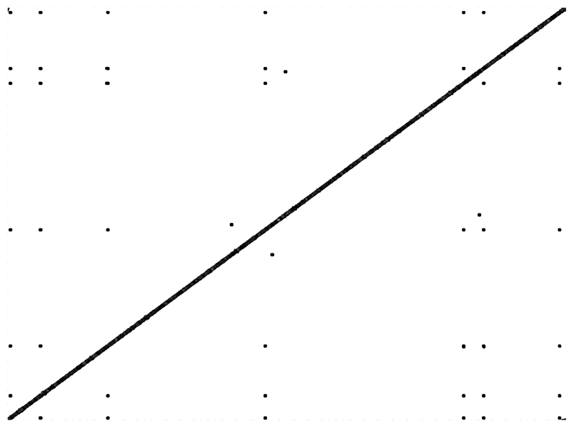
(a) A. baylyi simu. perfect 104X

(b) A. baylyi simu. raw 104X

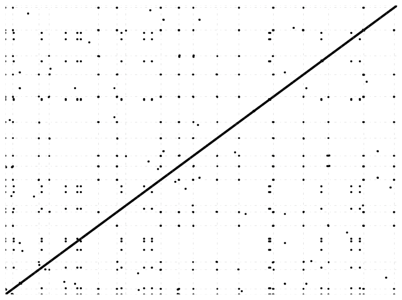
(c) S. cerevisiae simu. perfect 87x

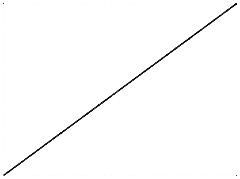
(d) A. baylyi sim. perfect 104X

(e) A. baylyi simu. raw 104X

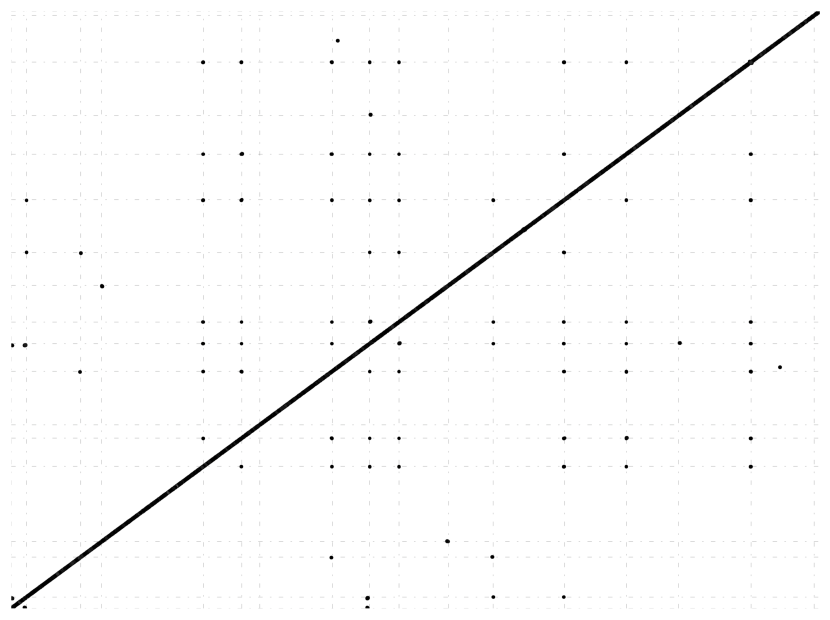
(f) S. cerevisiae simu. perfect 87x

Figure S3: Ordered similarity matrices for simulated datasets after removing 50% of the overlaps (a-c) or 90% (d-f) to illustrate the outlier removal by thresholding on the overlap score. The reads were simulated with NanoSim [Yang et al.,, 2016], from the A. baylyi ONT R7.3 and S. cerevisiae ONT R9 datasets. Subfigures 3(a) and 3(d) (respectively 3(c) and 3(f)) represent the similarity for reads generated with NanoSim from the A. baylyi ONT R7.3 (respectively S. cerevisiae ONT R9) dataset with option –perfect, which means these synthetic reads follow the same length distribution than the original dataset, but have no errors, and have the coverage specified above. The matrices 3(b) and 3(e) were generated from the A. baylyi ONT R7.3 dataset without the –perfect option, which means they have the same length and error distribution than the original data, but with higher coverage. For perfect and noisy synthetic A. baylyi reads and with sufficient coverage, all outliers could be removed by thresholding while keeping a connected similarity graph (all matrices in the Figure are connected). On the other hand, the similarity matrix generated with S. cerevisiae perfect reads still harbors a few outliers after removing 90% of the overlaps (with lowest score). When increasing the threshold value, the connectivity within some individual chromosomes will be broken before all outliers have been removed. Additional structural information (as used in Canu or Miniasm) will be required to resolve repeats in such situations.

Unfortunately, the correctly ordered (sorted by position of the reads on the backbone sequence) similarity matrix contains outliers outside the main diagonal band (see Figure 3) that corrupt the ordering. These outliers are typically caused by either repeated subsequences or sequencing noise (error in the reads and chimeric reads), although errors in the similarity can also be due to hashing approximations made in the overlap algorithm. We use a threshold on the similarity values and on the length of the overlaps to remove them. The error-induced overlaps are typically short and yield a low similarity score (e.g., number of shared min-mers), while repeat-induced overlaps can be as long as the length of the repeated region. By weighting the similarity, the value associated to repeat-induced overlaps can be lowered. Weighting can be done with, e.g., the --weighted option in MHAP to add a tf-idf style scaling to the MinHash sketch, making repetitive k-mers less likely to cause a match between two sequences, or with default parameters with minimap. In the Supplementary Material, we describe experiments with real, corrected and simulated reads to assess the characteristics of such overlaps and validate our method. Supplementary Figure S2 shows that although the overlap scores and lengths are lower for outliers than for inliers on average, the distributions of these quantities intersect. As shown in S3, the experiments indicate that all false-overlaps can be removed with a stringent threshold on the overlap length and score. However, removing all these short or low score overlaps will also remove many true overlaps. For bacterial genomes, the similarity graph can either remain connected or be broken into several connected components after a threshold-based outlier removal, depending on the initial coverage. Figure S3 illustrates the empirical observation that the coverage needs to be above 60x to keep the graph connected while removing all outliers. Most outliers can be similarly removed for real and synthetic data from S. cerevisiae, although a few outliers, probably harboring telomeric repeats, remain at the ends of chromosomes after thresholding.

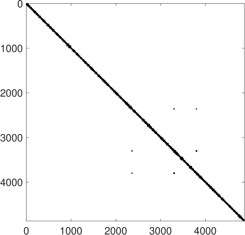
(a)

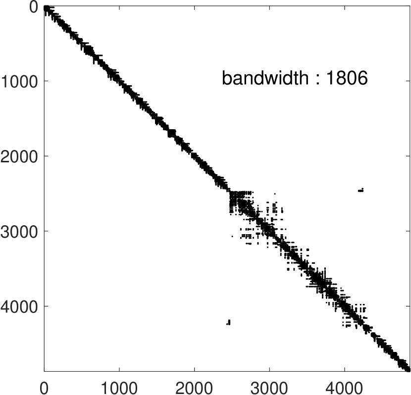
(b)

Figure S4: Similarity matrices containing outliers, displayed with true ordering (obtained by mapping the reads to the reference genome with GraphMap) and generated with a subset of A. baylyi ONT NanoSim perfect reads 4(a), and the same matrix incorrectly reordered with the spectral algorithm 4(b). The bandwidth is about 50 times as large as in the absence of outliers. This significant gap (an order of magnitude difference) between the bandwidth of the matrix reordered with the spectral algorithm depending on whether the original matrix (ordered by increasing position of the reads) contained outliers (i.e., is band-diagonal) or not motivated the development of the heuristic for assessing the ordering found by the spectral algorithm, as explained in §2.3. However, this heuristic is not applicable when the size of the similarity matrix is small, e.g., if the matrix is of size 100, the bandwidth cannot exceed 100 and the use of the heuristic is precluded.

There is thus a tradeoff to be reached depending on how many true overlaps one can afford to lose. With sufficient coverage, a stringent threshold on overlap score and length will remove both repeat-induced and error-induced overlaps, while still yielding a connected assembly graph. Otherwise, aggressive filtering will break the similarity graph into several connected components. In such a case, since the spectral algorithm only works with a connected similarity graph, we compute the layout and consensus separately in each connected component, resulting in several contigs. To set the threshold sufficiently high to remove outliers but small enough to keep the number of contigs minimal, we used a heuristic based on the following empirical observation, illustrated in Supplementary Figure S4. The presence of outliers in the correctly (based on the positions of the reads) ordered band diagonal matrix imparts an increased bandwidth (maximum distance to the diagonal of non zero entries) on the matrix reordered with the spectral algorithm.

We can therefore run the spectral algorithm, check the bandwidth in the reordered matrix, and increase the threshold if the bandwidth appears too large (typically larger than twice the coverage).

In practice, we chose to set the threshold on the overlap length to 3.5kbp, and removed the overlaps with the lowest score [in the first 40%-quantile (respectively 90% and 95%) for C$\leq$60X (resp. 60X$\leq$C$\leq$100X and C$\geq$100X)]. As indicated in Algorithm 2, we let these threshold values increase if indicated by the bandwitdh heuristic.

Finally, we added a filtering step to remove reads that have non-zero similarity with several sets of reads located in distant parts of the genome, such as chimeric reads. These reads usually overlap with a first subset of reads at a given position in the genome, and with another distinct subset of reads at another location, with no overlap between these distinct subsets. We call such reads “connecting reads”, and they can be detected from the similarity matrix by computing, for each read (index $i$), the set of its neighbors in the graph $\mathcal{N}_{i}=\{j:A_{ij}>0\}$. The subgraph represented by $A$ restricted to $\mathcal{N}_{i}$ is either connected (there exists a path between any pair of edges), or split into separate connected components. In the latter case, we keep the overlaps between read $i$ and its neighbor that belong to only one of these connected components (the largest one).

Algorithm 2 OLC assembly pipeline

0:  $n$ long noisy reads

1:  Compute overlaps with an overlapper (e.g. minimap or MHAP)

2:  Construct similarity matrix $S\in\mathbb{R}^{n\times n}$ from the overlaps

3:  Remove outliers from $S$ with a threshold on values $S_{ij}$, on overlap length, and removal of connecting reads (as explained in §6.3)

4:  for all Connected component $A$ of $S$ do

5:     Reorder $A$ with spectral algorithm (Algorithm 1)

6:     if bandwidth of $A_{reordered}$ $\geq$ 2$\times$ Coverage then

7:        set higher threshold on $A$ and try again

8:     end if

9:     Compute layout from the ordering found and overlaps

10:     Partition the length of the contig into small windows

11:     Compute consensus in each window with SPOA

12:     Merge consecutive windows with SPOA

13:  end for

13:  Contig consensus sequences

7 Results

7.1 Data

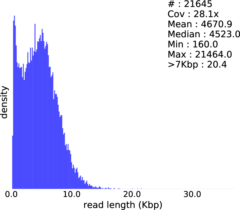
(a) A. baylyi ONT

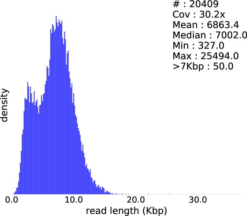
(b) E. coli ONT

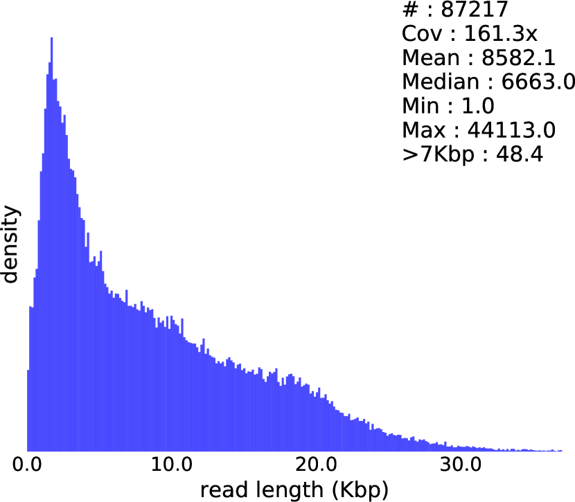
(c) E. coli PacBio

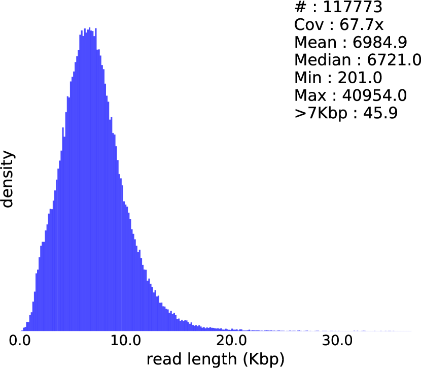
(d) S. cerevisiae ONT R7.3

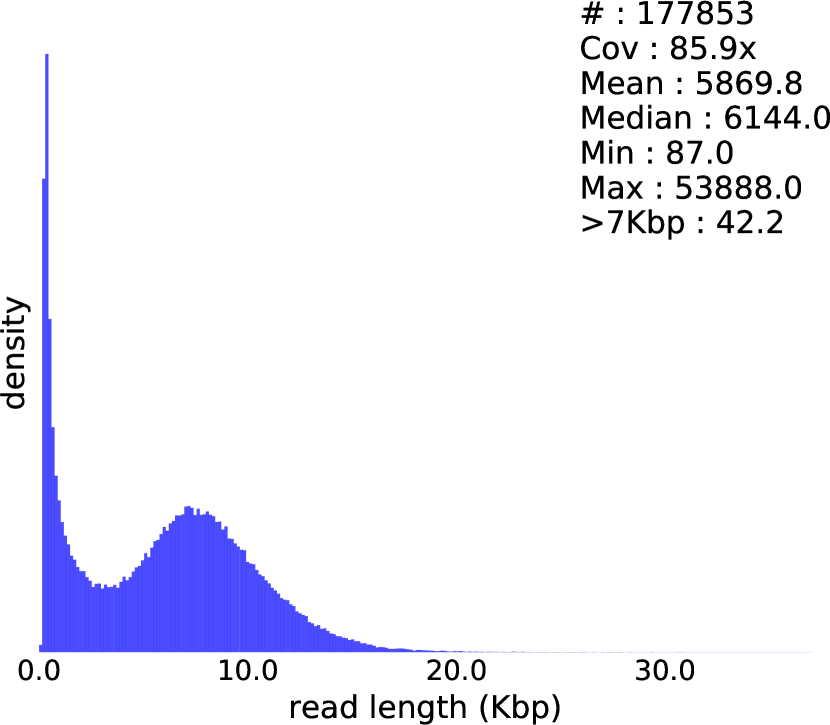
(e) S. cerevisiae ONT R9

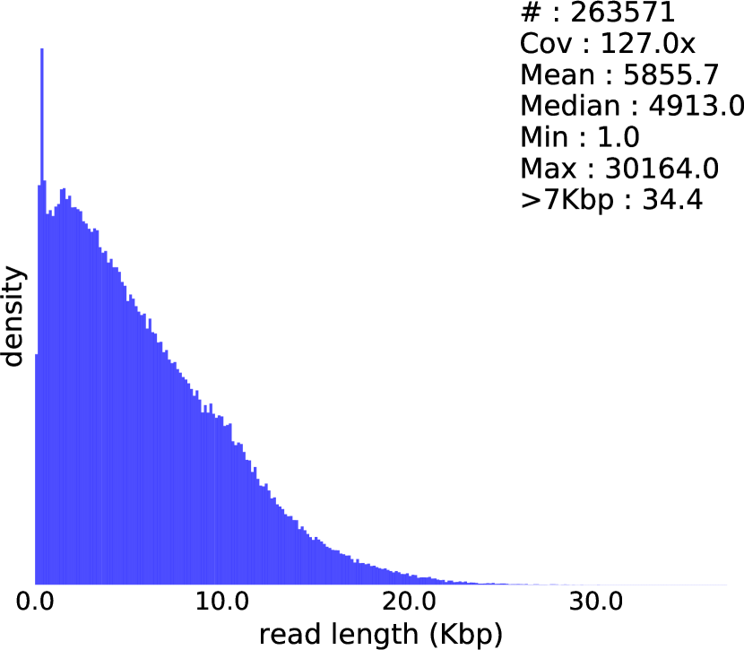
(f) S. cerevisiae PacBio

Figure S5: Read length histograms of the raw datasets.

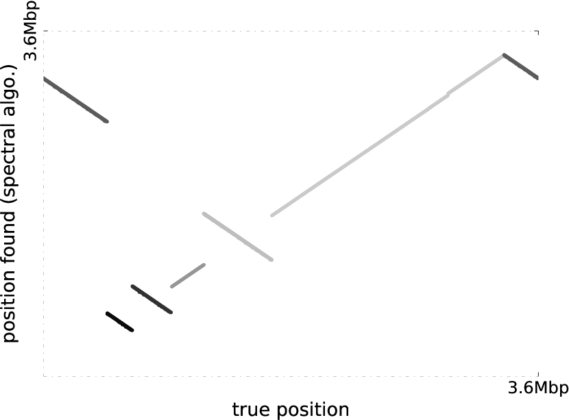
(a) A. baylyi ONT

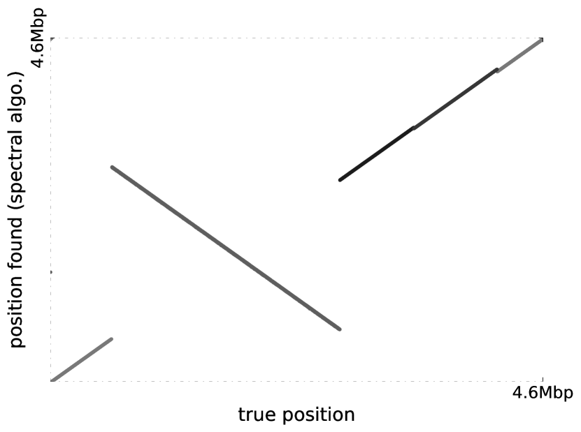
(b) E. coli ONT

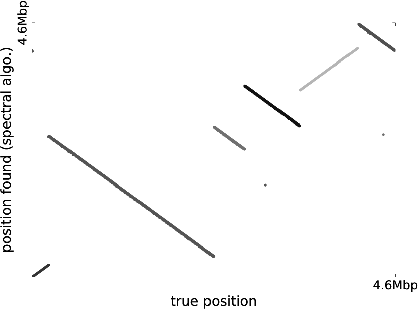
(c) E. coli PacBio

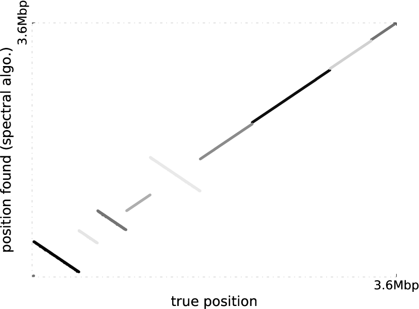
(d) A. baylyi ONT corr.

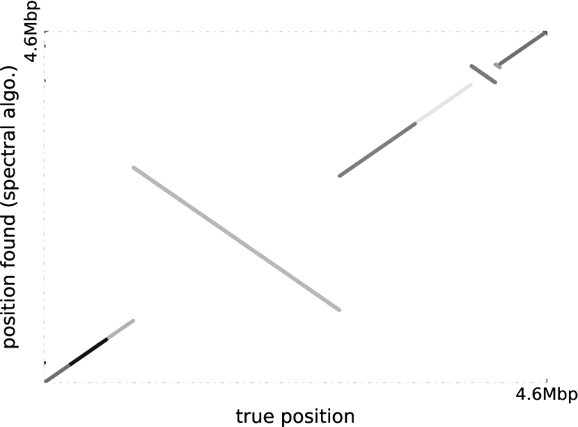
(e) E. coli ONT corr.

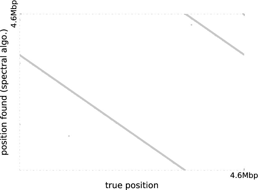
(f) E. coli PacBio corr.

Figure S6: Ordering of the reads computed with the spectral algorithm vs true ordering (obtained by mapping the reads to the reference genome with GraphMap) for the original (a-c) and corrected (d-f) bacterial datasets. All contigs are artificially displayed on the same plot for compactness.

We tested this pipeline on ONT and PacBio data. The bacterium Acinetobacter baylyi ADP1 and the yeast Saccharomyces cerevisiae S288C were sequenced at Genoscope with Oxford Nanopore’s MinION device using the R7.3 chemistry, together with an additional dataset of S. cerevisiae S288C using the R9 chemistry. Only the 2D high quality reads were used. The S. cerevisiae S288C ONT sequences were deposited at the European Nucleotide Archive (http://www.ebi.ac.uk/ena) where they can be accessed under Run accessions ERR1539069 to ERR1539080, while Acinetobacter baylyi ADP1 sequences will be made available on https://github.com/antrec/spectrassembler. We also used the following publicly available data: ONT Escherichia coli by Loman et al., [2015] (http://bit.ly/loman006 - PCR1 2D pass dataset), and PacBio E. coli K-12 PacBio P6C4, and S. cerevisiae W303 P4C2. Their key characteristics are given with the assembly results in Table 7.3.2, and read length histograms are given in Supplementary Figure S5. For each dataset, we also used the reads corrected and trimmed by the Canu pipeline as an additional dataset with low error-rate. The results on these corrected datasets are given in Supplementary Figures S6 and S7 and Tables 9 and 9.

7.2 Layout

7.2.1 Bacterial genomes

minimap was used to compute overlaps between raw reads (we obtained similar results with MHAP and DALIGNER). The similarity matrix preprocessed as detailed in Section6.3 yielded a few connected components for bacterial genomes. The reads were successfully ordered in each of these, as one can see in Figure 4 for E. coli, and in Figure S6 for the other datasets.

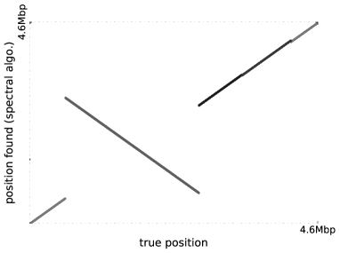
Figure 4: Ordering of the reads computed with the spectral algorithm vs true ordering (obtained by mapping the reads to the reference genome with GraphMap) for the E. coli ONT dataset. All contigs are artificially displayed on the same plot for compactness. There are two equivalent correct orderings for each contig : (1,2,…,n) and (n, n-1, …, 1), both yielding the same 2-SUM score (1) and leading to the same consensus sequence (possibly reverse complemented).

7.2.2 Eukaryotic genome

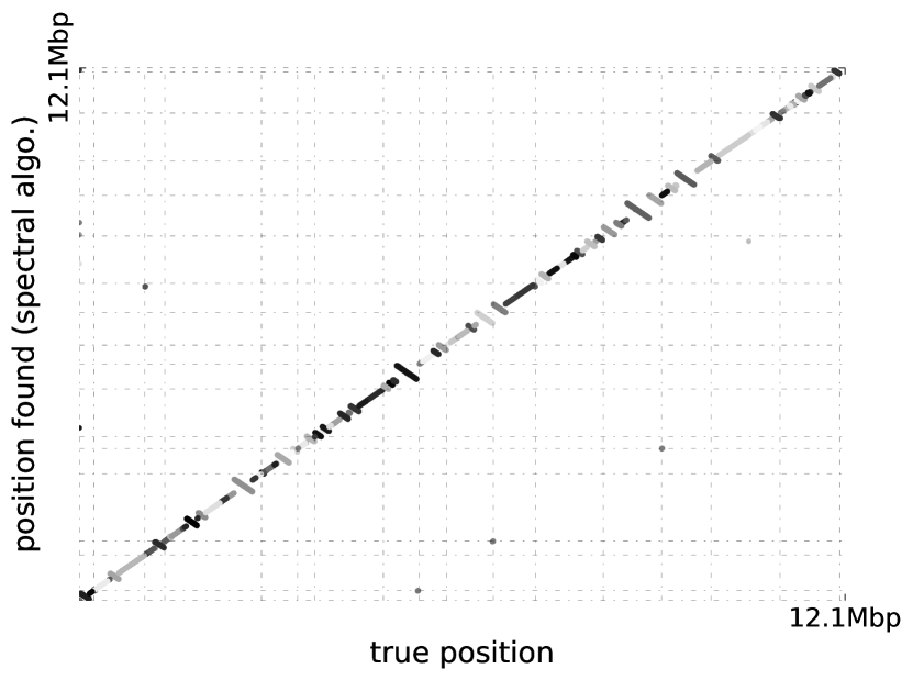
(a) ONT R7.3

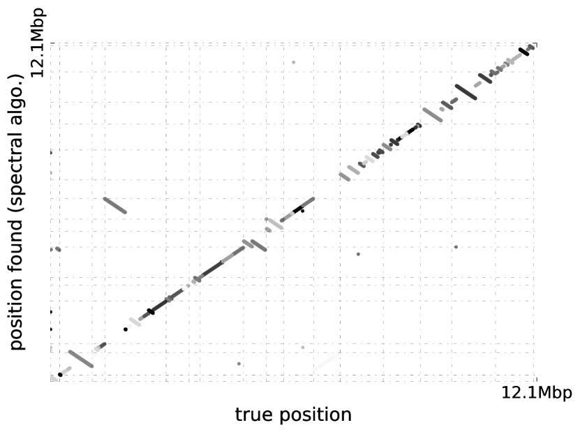
(b) ONT R9

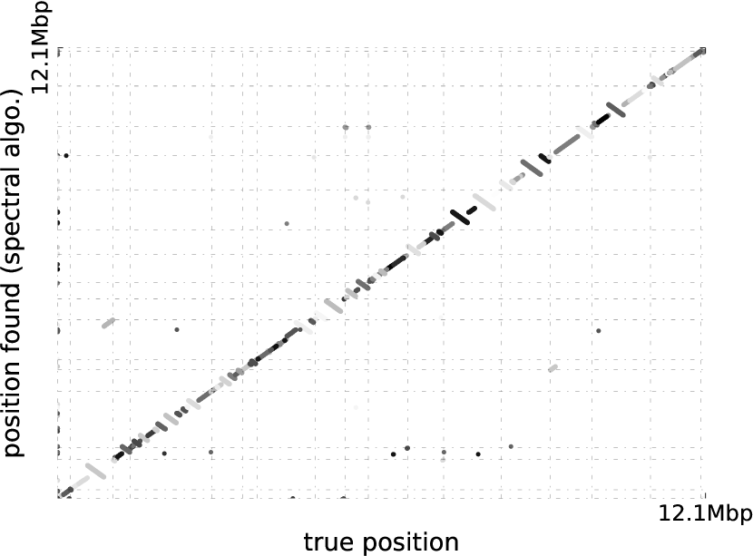
(c) PacBio

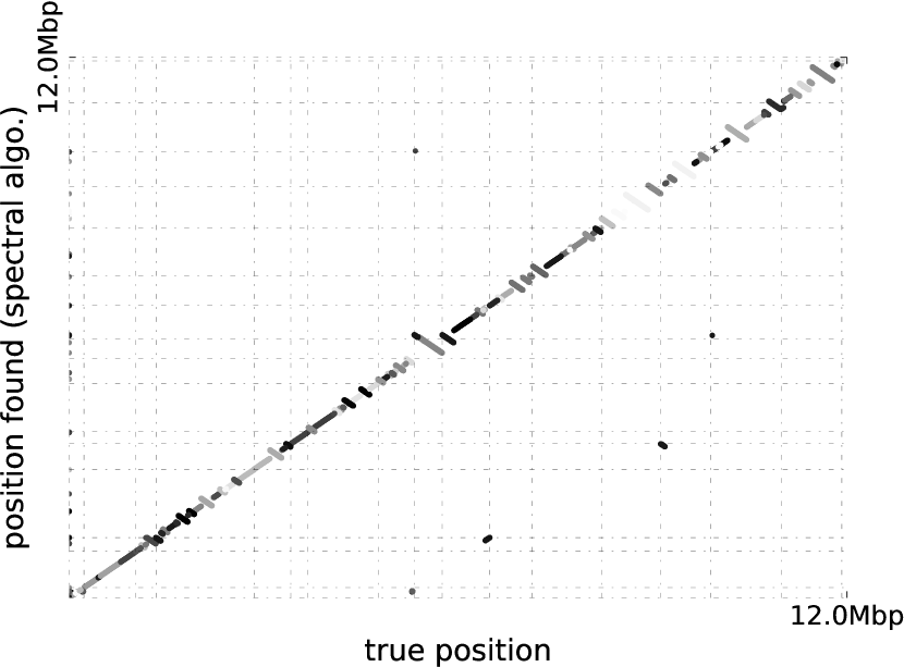
(d) ONT R7.3 corr.

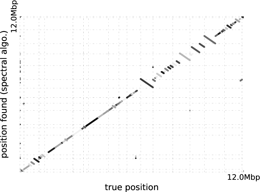
(e) ONT R9 corr.

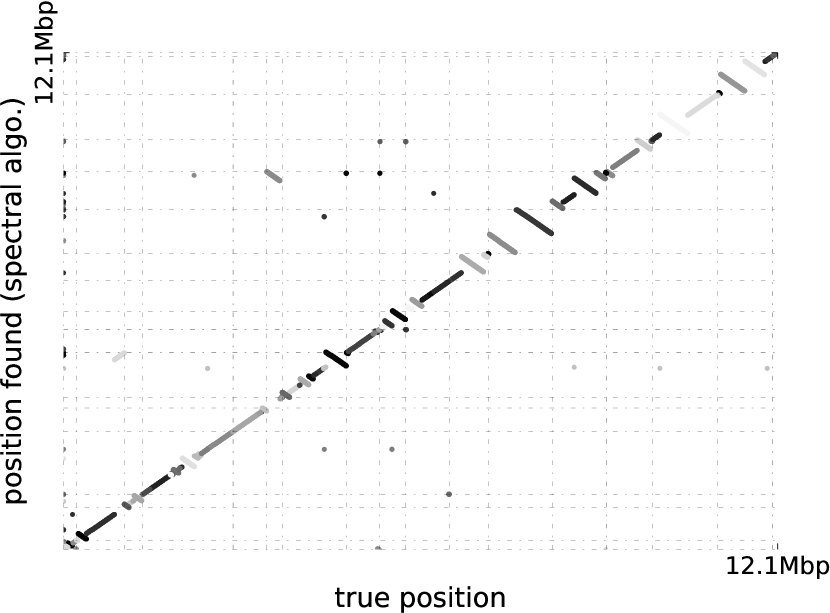
(f) PacBio corr.

Figure S7: Ordering of the reads computed with the spectral algorithm vs true ordering (obtained by mapping the reads to the reference genome with GraphMap) for the original (a-c) and corrected (d-f) yeast (S. cerevisiae) datasets. All contigs are artificially displayed on the same plot for compactness. The dashed lines represent the boundaries between chromosomes. The correction slightly improves the layout for the yeast genomes.

For the S. cerevisiae genome, the threshold on similarity had to be set higher than for bacterial genomes because of a substantially higher number of repetitive regions and false overlaps, leading to a more fragmented assembly. Most of them are correctly reordered with the spectral algorithm, see Figure 5 and Supplementary Figure S7.

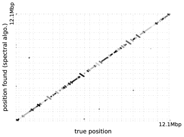
Figure 5: Ordering of the Saccharomyces cerevisiae ONT R7.3 reads identified with the spectral algorithm vs true ordering (obtained by mapping the reads to the reference genome with GraphMap and concatenating the ordering found in each chromosome). The different chromosomes are separated by grid lines.

7.3 Consensus

7.3.1 Recovering contiguity

Once the layout was established, the method described above was used to assemble the contigs and generate a consensus sequence. For the two bacterial genomes, the first round of layout produced a small number of connected components, each of them yielding a contig. Sufficient overlap was left between the contig sequences to find their layout with a second iteration of the algorithm and produce a single contig spanning the entire genome. The number of contigs in the yeast assemblies can be reduced similarly. The fact that the first-pass contigs overlap even though they result from breaking the similarity graph into several connected components might seem counter-intuitive at first sight. However, note that when cutting an edge $A_{ij}$ results in the creation of two contigs (one containing $i$ and the other $j$), the sequence fragment at the origin of the overlap between the two reads is still there on both contigs to yield an overlap between them in the second iteration. Alternatively, we found the following method useful to link the contigs’ ends: 1. extract the ends of the contig sequences, 2. compute their overlap with minimap, 3. propagate the overlaps to the contig sequences, 4. use miniasm with all pre-selection parameters and thresholds off, to just concatenate the contigs (see Supplementary Material §9).

7.3.2 Consensus quality evaluation

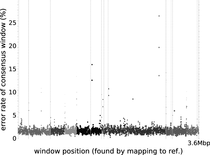
(a) A. baylyi ONT

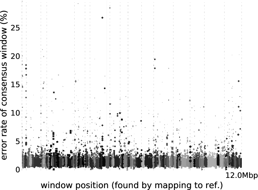
(b) S. cerevisiae ONT R7.3

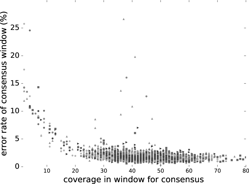
(c) A. baylyi ONT

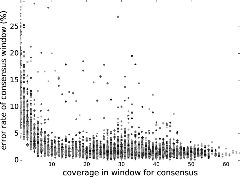
(d) S. cerevisiae ONT R7.3

Figure S9: Error-rates in consensus windows versus position of the windows on the reference genome (a,b). The dashed lines represent the location of repeats for A. baylyi, and the separation between chromosomes for S. cerevisiae. The size of each scatter marker is proportional to the coverage of the window. The (c,d) panel represents the error-rates in consensus windows versus the coverage of the windows. The error-rate was computed with the errorrates.py script from samtools, using the mapping obtained from GraphMap. Most of the windows with a high error rate are positioned at the ends of the contigs they belong to. We also observed that repeats are often positioned at the edge between two contigs, though this does not seem to be the determinant factor. The bottom plots represent the error-rate in the windows against their estimated coverage, defined as the total length of sequences used to perform the multiple alignment in the window normalized by the length of the consensus sequence. Overall, one can see that the windows with high error rate are the ones with low coverage. Nevertheless, especially for the yeast genomes, there are also several windows with high values for both error-rate and coverage. Manual inspection of these reveals that they usually do not span repeated regions, but their high error-rates arise from imperfections in the layout.

We first investigated the quality of the consensus sequences derived in each window. Figures 6 and S8 highlight the correcting effect of the consensus. Supplementary Figure S9 suggests that the error-rate in the consensus windows depends mainly on the local coverage. We then compared our results to those obtained with other long reads assemblers : Miniasm, Canu and Racon [Vaser et al.,, 2016]. Racon takes a draft assembly, the raw reads, and a mapping of the reads to the draft assembly as input. We used it with the draft assembly produced by Miniasm (as done by Vaser et al., [2016]). We label this method “Miniasm+Racon” in our results. We also used Racon with the draft assembly derived by our method (“Spectral+Racon” method), using Minimap to map the raw reads to the draft assemblies before using Racon. A summary of assembly reports generated with DNAdiff [Kurtz et al.,, 2004] and QUAST [Gurevich et al.,, 2013] are given in Table 7.3.2 and Supplementary Table 9. Briefly, the assemblies displayed between $98\%$ and $99\%$ average identity to their reference genome, with errors mostly consisting in deletions. Misassemblies were rare in reconstructed bacterial genomes but more frequent in assembled yeast genomes, where they mostly consisted in translocations and relocations caused by either deletions and/or misplaced reads in the layout.

Assembly results of the spectral method, compared to Miniasm, Canu and Racon, across the different datasets Miniasm Spectral Canu Miniasm+Racon Miniasm+Racon (2 iter.) Spectral+Racon A. baylyi ONT R7.3 28x Ref. genome size [bp] 3598621 3598621 3598621 3598621 3598621 3598621 Total bases [bp] 3531295 3551582 3513432 3564823 3566438 3551094 Ref. chromosomes [#] 1 1 1 1 1 1 Contigs [#] 5 1 (7) 1 5 5 1 (7) Aln. bases ref [bp] 3445457(95.74%) 3596249(99.93%) 3595082(99.90%) 3596858(99.95%) 3596854(99.95%) 3598181(99.99%) Aln. bases query [bp] 3379002(95.69%) 3549290(99.94%) 3513081(99.99%) 3564455(99.99%) 3566021(99.99%) 3550742(99.99%) Misassemblies [#] 0 0 2 2 2 0 Avg. identity 87.31 98.17 97.59 98.18 98.36 98.42 E. coli ONT R7.3 30x Ref. genome size [bp] 4641652 4641652 4641652 4641652 4641652 4641652 Total bases [bp] 4759346 4662043 4625543 4647066 4643235 4629112 Ref. chromosomes [#] 1 1 1 1 1 1 Contigs [#] 3 1 (4) 2 3 3 1 (4) Aln. bases ref [bp] 4355121(93.83%) 4612515(99.37%) 4638255(99.93%) 4640127(99.97%) 4640127(99.97%) 4641457(100.00%) Aln. bases query [bp] 4432658(93.14%) 4623823(99.18%) 4625535(100.00%) 4642837(99.91%) 4639816(99.93%) 4628962(100.00%) Misassemblies [#] 0 2 8 3 3 2 Avg. identity 89.28 98.80 99.40 99.31 99.45 99.46 S. cerevisiae ONT R7.3 68x Ref. genome size [bp] 12157105 12157105 12157105 12157105 12157105 12157105 Total bases [bp] 11813544 12213218 12142953 11926664 11926191 12167363 Ref. chromosomes [#] 17 17 17 17 17 17 Contigs [#] 29 71 (127) 36 29 29 71 (127) Aln. bases ref [bp] 11566318(95.14%) 12043050(99.06%) 12086977(99.42%) 12084923(99.41%) 12086556(99.42%) 12061384(99.21%) Aln. bases query [bp] 11236806(95.12%) 12134480(99.36%) 12089056(99.56%) 11923058(99.97%) 11918621(99.94%) 12135284(99.74%) Misassemblies [#] 0 7 34 18 19 11 Avg. identity 89.00 98.00 98.33 98.49 98.63 98.61 S. cerevisiae ONT R9 86x Ref. genome size [bp] 12157105 12157105 12157105 12157105 12157105 12157105 Total bases [bp] 11734150 11795644 12217497 12128279 12129086 11750114 Ref. chromosomes [#] 17 17 17 17 17 17 Contigs [#] 30 48 (85) 26 30 29 48 (85) Aln. bases ref [bp] 11947453(98.28%) 11607131(95.48%) 12126980(99.75%) 12126663(99.75%) 12127467(99.76%) 11695983(96.21%) Aln. bases query [bp] 11549494(98.43%) 11668882(98.93%) 12179843(99.69%) 12118506(99.92%) 12121202(99.93%) 11717047(99.72%) Misassemblies [#] 0 23 39 18 19 36 Avg. identity 93.55 98.81 99.02 99.16 99.20 99.10 E. coli PacBio 161x Ref. genome size [bp] 4641652 4641652 4641652 4641652 4641652 4641652 Total bases [bp] 4845211 4731239 4670125 4653228 4645420 4674460 Ref. chromosomes [#] 1 1 1 1 1 1 Contigs [#] 1 2 (6) 1 1 1 2 (6) Aln. bases ref [bp] 4437473(95.60%) 4617713(99.48%) 4641652(100.00%) 4641551(100.00%) 4641500(100.00%) 4641652(100.00%) Aln. bases query [bp] 4601587(94.97%) 4705704(99.46%) 4670125(100.00%) 4653140(100.00%) 4645420(100.00%) 4673065(99.97%) Misassemblies [#] 0 5 4 4 4 4 Avg. identity 89.13 98.63 99.99 99.64 99.91 99.87 S. cerevisiae PacBio 127x Ref. genome size [bp] 12157105 12157105 12157105 12157105 12157105 12157105 Total bases [bp] 12266420 12839034 12346258 12070971 12052148 12695031 Ref. chromosomes [#] 17 17 17 17 17 17 Contigs [#] 30 90 (136) 29 30 30 90 (136) Aln. bases ref [bp] 11250453(92.54%) 11917823(98.03%) 12091868(99.46%) 12023040(98.90%) 12024968(98.91%) 12002816(98.73%) Aln. bases query [bp] 11396172(92.91%) 12456415(97.02%) 12304982(99.67%) 12045088(99.79%) 12027812(99.80%) 12485128(98.35%) Misassemblies [#] 0 57 76 61 59 68 Avg. identity 88.29 98.41 99.87 99.43 99.72 99.54 For the spectral method, we give the results after contig merging (see §7.3.1); the number of contigs before this post-processing is given between parentheses. Racon’s use here can be seen as a polishing phase for the sequences outputted by the spectral method and Miniasm. To keep both assemblers on an equal footing, we compared Spectral+Racon to two iterations of Miniasm+Racon (since one pass of Miniasm does not implement any consensus). The best results in terms of average identity are highlighted in bold (but other metrics should also be used to compare the assemblies). Canu clearly outperforms the spectral method on PacBio data, while both assemblers yield comparable results on the ONT datasets.

Figure 6: Error rate of consensus window sequences, compared to the raw and corrected (with the Canu correction and trimming modules) reads for the A. baylyi ONT dataset. The error rates were computed by mapping the sequences to the A. baylyi reference genome. Histograms for the other datasets are available in Supplementary Figure S8.

7.3.3 Optical mapping

After the first iteration of the bacterial genome assembly pipeline, overlaps between the first-pass contigs were sufficient to find their layout. It should be anticipated however that not all overlaps might be apparent in some cases, e.g. if too many reads were removed during the preprocessing step. One attractive option is to use optical mapping [Aston et al.,, 1999] to layout the contigs. We had such an optical map available for the A. baylyi genome, and implemented the algorithm of Nagarajan et al., [2008] to map the contigs to the restriction map, which led to the same layout as the one identified from our two-round assemblies (data not shown), thus providing a “consistency check” for the layout. We suggest in Supplementary Figure S10 and Table S1 that optical maps could be particularly valuable for the ordering of contigs from more structurally complex eukaryotic genomes such as S. cerevisiae.

8 Discussion

We have shown that seriation based layout algorithms can be successfully applied to de novo genome assembly problems, at least for genomes harboring a limited number of repeats.

In a similar vein to the recent report about the miniasm assembly engine [Li,, 2016], our work confirms that the layout of long reads can be found without prior error correction, using only overlap information generated from raw reads by tools such as minimap, MHAP or DALIGNER. However, unlike miniasm, which does not derive a consensus but instead concatenates the reads into a full sequence, we take advantage of read coverage to produce contigs with a consensus quality on par with that achieved by assembly pipelines executing dedicated error-correction steps. The results of Table 7.3.2 appear promising. For example, our assembler combined with Racon yields among the highest average identities with the reference for the ONT datasets. In terms of speed however, our pipeline is clearly outperformed by Miniasm, but also by Miniasm+Racon, the latter improving overall accuracy. Still, compared to approaches implementing error correction steps, we gain significant speed-ups by highly localizing the error correction and consensus generation processes, which is made possible by knowledge of the layout. We believe that tools such as Miniasm and Racon are implemented in a much more efficient way than our own, but the layout method itself is efficient (see Supplementary Table 9) and is known to be scalable as it relies on the same algorithmic core as Google’s PageRank.

The main limitation of our layout algorithm is its sensitivity to outliers in the similarity matrix, hence the need to remove them in a pre-processing phase. Higher coverage and quality of the input reads, both expected in the near future, would likely improve the robustness of our pipeline. Still, for eukaryotic genomes, we found that some outliers require additional information to be resolved (see Supplementary FigureS3), which could be provided in the future by extracting topological information from the assembly graph.

In the meantime, our pipeline behaves like a draft generating assembler for prokaryotic genomes, and a first-pass unitigger for eukaryotic genomes. Importantly, the overall approach is modular and can integrate other algorithms to increase layout robustness or consensus quality, as illustrated here by the integration of Racon as an optional polishing module.

Our original contribution here consists in the layout computation. The spectral OLC assembler we built on top of it could be enhanced in many ways. We have shown that the spectral algorithm is suited to find the layout for bacterial genomes, even though there is room left for performance improvements on repeat-rich eukaryotic genomes.

For these eukaryotic genomes, it could make sense to use the spectral algorithm jointly with other assembly engines (e.g. Miniasm or Canu), to check the consistency of connected components before they are assembled. Our consensus generation method is coarse-grained for now and does not take into account statistical properties of ONT sequencing errors. Nevertheless, the three components (O, L and C) of the method being independent, an external and more refined consensus generation process could readily be plugged after the overlap and layout computations to further improve results and increase accuracy.

9 Supplementary Material

Running time for the different methods on the datasets presented in Section7.1 Spectral Layout Spectral (full, +Minimap) Canu Minimap + Miniasm Racon after Miniasm Racon after Spectral A. baylyi ONT R7.3 28x Runtime [h:mm:ss] 0:00:23 (0:00:59) 0:12:52 0:25:55 0:00:28 0:01:54 0:01:48 Max mem [Gb] 1.966 1.966 3.827 1.499 0.756 0.484 E. coli ONT R7.3 30x Runtime [h:mm:ss] 0:00:41 (0:01:25) 0:16:15 0:28:40 0:00:13 0:04:36 0:02:14 Max mem [Gb] 1.216 1.216 4.655 2.099 0.879 0.645 S. cerevisiae ONT R7.3 68x Runtime [h:mm:ss] 0:01:41 (0:07:60) 1:41:20 4:33:08 0:01:17 0:21:11 0:21:32 Max mem [Gb] 12.208 12.208 4.015 8.506 2.376 2.325 S. cerevisiae ONT R9 86x Runtime [h:mm:ss] 0:03:38 (0:09:28) 2:26:44 7:15:41 0:02:14 0:23:09 0:22:03 Max mem [Gb] 32.928 32.928 3.986 12.397 2.966 2.775 E. coli PacBio 161x Runtime [h:mm:ss] 0:05:19 (0:05:44) 1:32:13 0:51:32 0:01:16 0:16:51 0:18:18 Max mem [Gb] 21.650 21.650 3.770 9.969 8.082 4.619 S. cerevisiae PacBio 127x Runtime [h:mm:ss] 0:03:11 (0:07:01) 2:59:41 1:50:23 0:02:10 0:20:54 0:23:32 Max mem [Gb] 32.184 32.184 3.810 16.881 4.290 4.307 Run-time and peak memory for the previously compared methods, when run on a 24 cores Intel Xeon E5-2640 2.50GHz node. Runtime and Max mem correspond to the wall-clock and maximum resident set size fields of the unix /usr/bin/time -v command. The first column (Spectral Layout) displays the running time of the layout phase of our method in the following way: time to reorder contigs with the spectral algorithm (total time to get fine-grained layout); the total time for the layout (including the fine-grained computation of the position of the reads on a backbone sequence) is given between parentheses next to the time for the ordering. The second column gives the runtime for our full pipeline, including running minimap to obtain the overlaps. The runtime for Racon includes the time to map the reads to the backbone sequence with Minimap and to run Racon for the consensus (Racon requires a backbone sequence, obtained either with Miniasm or Spectral in the present experiments). Indeed, the Racon pipeline maps the reads to a draft sequence to get the layout and then computes consensus sequences in windows across the genome. Our pipeline instead directly computes the layout and then generates consensus sequences in windows across the genome (the latter task being embarassingly parallel). Canu is faster than our method on the PacBio datasets (probably at least because because we did not adapt our pipeline (as Canu does) to the much higher coverage, nor to the higher fraction of chimeric reads typical of PacBio data), but not on the ONT datasets. The memory for the spectral method can be allocated among several cores.

Figure S1: Runtime of the spectral ordering algorithm in connected components of different sizes (across all datasets), with two solvers for the eigenvalues computations (scipy.sparse.eigsh and the eigs function from Julia [Bezanson et al.,, 2017]). We implemented a call to Julia for matrices of size larger than 3000 in the code since its eigenvector computation scales better for large matrices (probably due to the fact that the matrices are passed by reference in Julia) but has a non-negligible overhead for small matrices.

Assembly results of several assemblers across the datasets corrected with Canu Miniasm Spectral Canu Miniasm+Racon Miniasm+Racon (2 iter.) Spectral+Racon A. baylyi ONT R7.3 28x (26x) Ref. genome size [bp] 3598621 3598621 3598621 3598621 3598621 3598621 Total bases [bp] 3493724 3523055 3516777 3540178 3540766 3522315 Ref. chromosomes [#] 1 1 1 1 1 1 Contigs [#] 5 2 (9) 2 5 5 2 (9) Aln. bases ref [bp] 3594663(99.89%) 3596069(99.93%) 3595264(99.91%) 3595193(99.90%) 3595193(99.90%) 3596269(99.93%) Aln. bases query [bp] 3492976(99.98%) 3522804(99.99%) 3516440(99.99%) 3539856(99.99%) 3540444(99.99%) 3522311(100.00%) Misassemblies [#] 2 1 2 2 2 1 Avg. identity 96.40 97.87 97.61 97.79 97.85 97.86 E. coli ONT R7.3 30x (27x) Ref. genome size [bp] 4641652 4641652 4641652 4641652 4641652 4641652 Total bases [bp] 4597538 4613973 4627578 4617120 4617100 4613521 Ref. chromosomes [#] 1 1 1 1 1 1 Contigs [#] 3 1 (8) 2 3 3 1 (8) Aln. bases ref [bp] 4639179(99.95%) 4639815(99.96%) 4639396(99.95%) 4639355(99.95%) 4639355(99.95%) 4639420(99.95%) Aln. bases query [bp] 4597389(100.00%) 4613972(100.00%) 4627577(100.00%) 4617119(100.00%) 4617099(100.00%) 4613520(100.00%) Misassemblies [#] 2 2 4 2 2 2 Avg. identity 98.89 99.43 99.41 99.42 99.43 99.43 S. cerevisiae ONT R7.3 68x (38x) Ref. genome size [bp] 12157105 12157105 12157105 12157105 12157105 12157105 Total bases [bp] 11814836 11959669 12112186 11877015 11876882 11949674 Ref. chromosomes [#] 17 17 17 17 17 17 Contigs [#] 29 67 (126) 37 28 28 67 (126) Aln. bases ref [bp] 12061456(99.21%) 11963869(98.41%) 12068379(99.27%) 12062161(99.22%) 12061809(99.22%) 11969742(98.46%) Aln. bases query [bp] 11814252(100.00%) 11930637(99.76%) 12069253(99.65%) 11876268(99.99%) 11876225(99.99%) 11925068(99.79%) Misassemblies [#] 19 22 26 20 20 24 Avg. identity 97.81 98.32 98.36 98.39 98.39 98.38 S. cerevisiae ONT R9 86x (40x) Ref. genome size [bp] 12157105 12157105 12157105 12157105 12157105 12157105 Total bases [bp] 11946760 12081487 12184545 11970672 11970529 12061759 Ref. chromosomes [#] 17 17 17 17 17 17 Contigs [#] 21 65 (108) 30 20 20 65 (108) Aln. bases ref [bp] 12055448(99.16%) 11851023(97.48%) 12110461(99.62%) 12056562(99.17%) 12056734(99.17%) 11879607(97.72%) Aln. bases query [bp] 11944969(99.99%) 12043650(99.69%) 12184122(100.00%) 11970041(99.99%) 11969729(99.99%) 12040521(99.82%) Misassemblies [#] 21 32 26 22 22 38 Avg. identity 98.83 98.90 99.06 99.06 99.05 99.04 E. coli PacBio 161x (38x) Ref. genome size [bp] 4641652 4641652 4641652 4641652 4641652 4641652 Total bases [bp] 4642736 4663427 4670125 4642423 4642443 4662179 Ref. chromosomes [#] 1 1 1 1 1 1 Contigs [#] 1 1 (1) 1 1 1 1 (1) Aln. bases ref [bp] 4639048(99.94%) 4640514(99.98%) 4641652(100.00%) 4641623(100.00%) 4641616(100.00%) 4641652(100.00%) Aln. bases query [bp] 4639955(99.94%) 4662891(99.99%) 4670125(100.00%) 4642423(100.00%) 4642443(100.00%) 4662172(100.00%) Misassemblies [#] 2 4 4 4 4 4 Avg. identity 99.59 99.97 99.99 99.99 99.99 99.99 S. cerevisiae PacBio 127x (37x) Ref. genome size [bp] 12157105 12157105 12157105 12157105 12157105 12157105 Total bases [bp] 12174558 12232964 12346261 12194786 12193481 12217702 Ref. chromosomes [#] 17 17 17 17 17 17 Contigs [#] 26 55 (86) 29 26 26 55 (86) Aln. bases ref [bp] 12036689(99.01%) 12008560(98.78%) 12091871(99.46%) 12042104(99.05%) 12041381(99.05%) 12018488(98.86%) Aln. bases query [bp] 12151704(99.81%) 12179852(99.57%) 12304982(99.67%) 12177020(99.85%) 12175701(99.85%) 12172316(99.63%) Misassemblies [#] 74 75 76 76 76 80 Avg. identity 99.22 99.78 99.87 99.88 99.88 99.86 These corrected datasets were obtained by running Canu with the saveReadCorrections=True option on the datasets presented in 7.1. Canu includes correction and trimming, resulting in a removal of short reads and a lower coverage than in the original raw data. However, it is the coverage of the raw dataset which is relevant since higher coverage in the latter will result in longer reads in the corrected data, even though the coverage in all corrected datasets are roughly below 40x. We indicate the coverage of the corrected datasets in parentheses next to the coverage of the original dataset. For the spectral method, we give the results after the contig merging step (see 7.3.1). The number of contigs before this post-processing is given between parentheses. Unlike with raw data, the polishing effect of adding Racon to our pipeline is not significant. All methods have comparable results on the corrected datasets. The best result in terms of average identity only is indicated in bold (but other metrics should also be used to compare the assemblies).

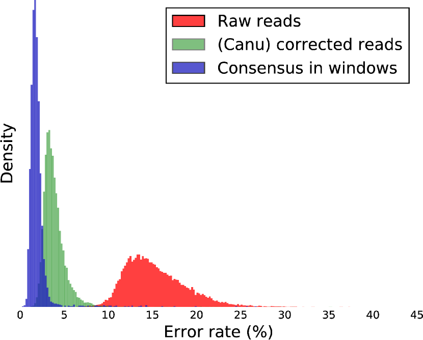
(a) A. baylyi ONT

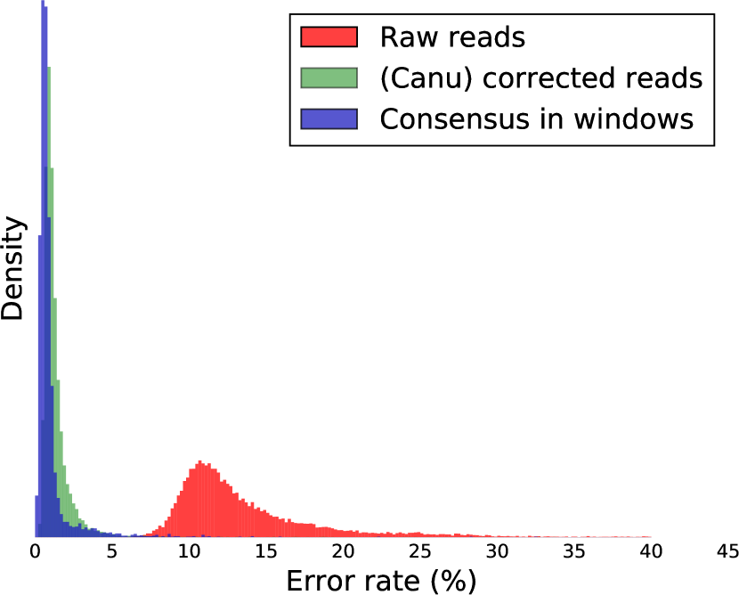
(b) E. coli ONT

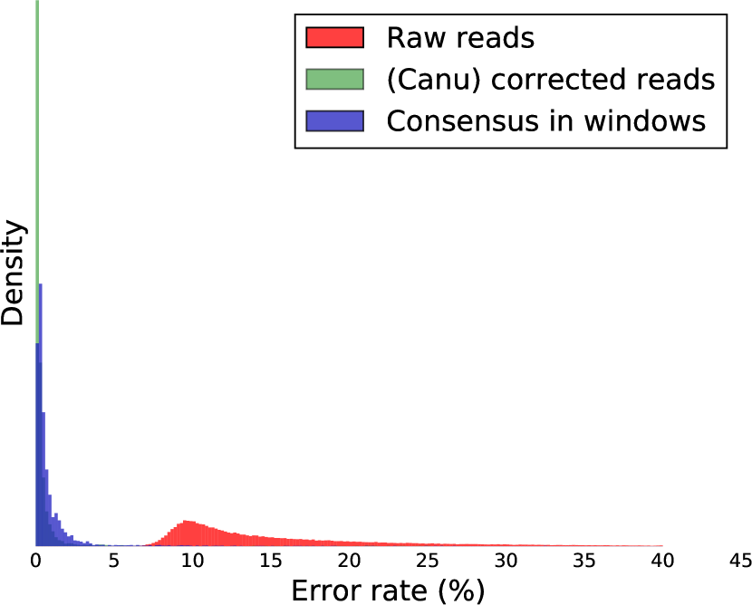
(c) E. coli PacBio

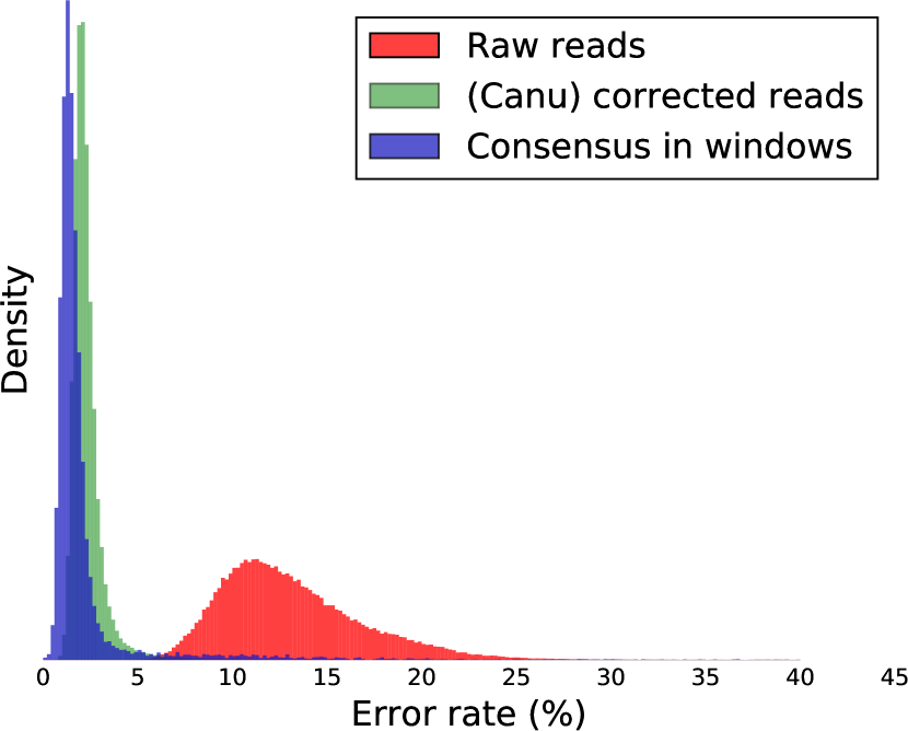
(d) S. cerevisiae ONT R7.3

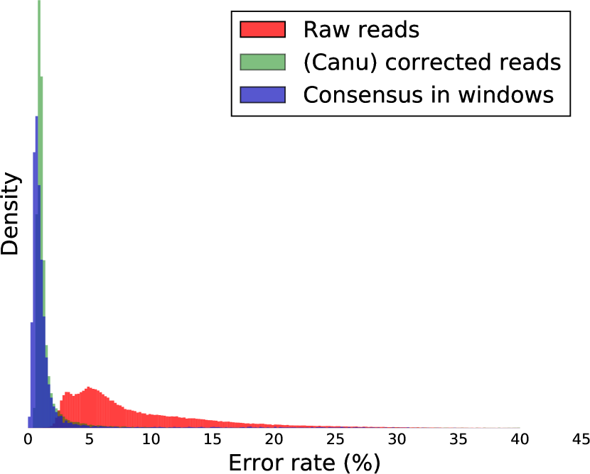
(e) S. cerevisiae ONT R9

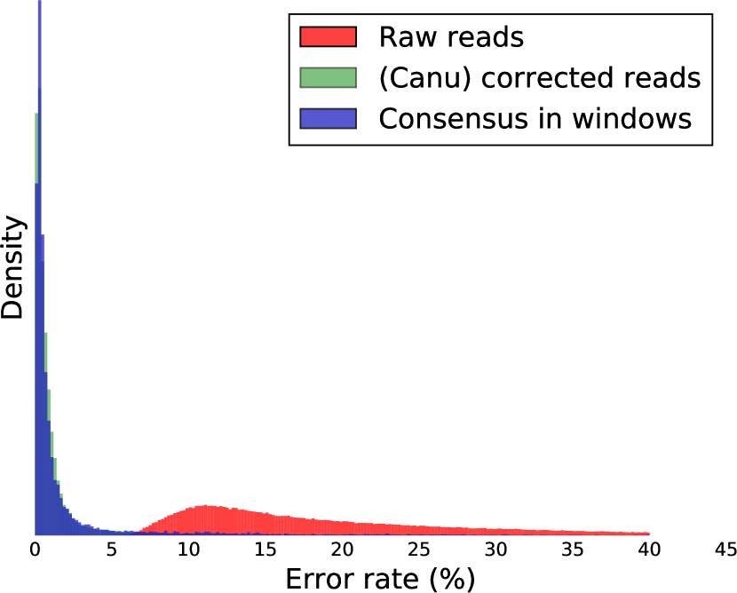
(f) S. cerevisiae PacBio

Figure S8: Error-rates in consensus windows, raw reads and corrected reads for the six real datasets. With ONT R7.3 data, the consensus produced by our pipeline appears more accurate than via the correction module of Canu, while the contrary is true for PacBio data.

Misassemblies report of the different assemblers across the various datasets Miniasm Spectral Canu Miniasm+Racon Miniasm+Racon (2 iter.) Spectral+Racon A. baylyi ONT R7.3 28x Relocations [#] 0 0 2 2 2 0 Translocations [#] 0 0 0 0 0 0 Inversions [#] 0 0 0 0 0 0 Missmbld. contigs [#] 0 0 1 1 1 0 Missmbld. contigs length [bp] 0 0 3513432 1993457 1994286 0 Local misassemblies [#] 0 7 5 0 0 0 Mismatches [#] 0 0 0 0 0 0 Indels [#] 0 0 0 0 0 0 Indels length [bp] 0 0 0 0 0 0 E. coli ONT R7.3 30x Relocations [#] 0 2 6 3 3 2 Translocations [#] 0 0 0 0 0 0 Inversions [#] 0 0 2 0 0 0 Missmbld. contigs [#] 0 1 2 2 2 1 Missmbld. contigs length [bp] 0 2160837 4625543 3743081 3740186 2148788 Local misassemblies [#] 0 50 2 2 2 3 Mismatches [#] 0 55 0 0 0 0 Indels [#] 0 1 1 0 0 0 Indels length [bp] 0 30 1 0 0 0 S. cerevisiae ONT R7.3 68x Relocations [#] 0 0 17 6 7 1 Translocations [#] 0 7 17 12 12 10 Inversions [#] 0 0 0 0 0 0 Missmbld. contigs [#] 0 7 16 11 11 10 Missmbld. contigs length [bp] 0 1223452 4852688 4638491 4638515 909031 Local misassemblies [#] 0 57 17 9 10 12 Mismatches [#] 0 63 0 0 0 0 Indels [#] 0 3 2 3 2 1 Indels length [bp] 0 90 124 167 132 54 S. cerevisiae ONT R9 86x Relocations [#] 0 5 22 9 9 4 Translocations [#] 0 18 17 9 10 32 Inversions [#] 0 0 0 0 0 0 Missmbld. contigs [#] 0 11 11 10 11 10 Missmbld. contigs length [bp] 0 3149392 5957900 4545988 4563372 2661541 Local misassemblies [#] 0 41 88 11 11 30 Mismatches [#] 0 0 0 0 0 0 Indels [#] 0 2 4 3 3 2 Indels length [bp] 0 161 250 208 207 157 E. coli PacBio 161x Relocations [#] 0 3 2 2 2 2 Translocations [#] 0 0 0 0 0 0 Inversions [#] 0 2 2 2 2 2 Missmbld. contigs [#] 0 1 1 1 1 1 Missmbld. contigs length [bp] 0 2848876 4670125 4653228 4645420 2818134 Local misassemblies [#] 0 66 2 3 2 2 Mismatches [#] 0 0 0 0 0 0 Indels [#] 0 0 0 1 0 0 Indels length [bp] 0 0 0 66 0 0 S. cerevisiae PacBio 127x Relocations [#] 0 17 31 21 20 18 Translocations [#] 0 40 44 39 38 50 Inversions [#] 0 0 1 1 1 0 Missmbld. contigs [#] 0 28 24 22 21 31 Missmbld. contigs length [bp] 0 6470761 10214689 9569247 9421896 6683508 Local misassemblies [#] 0 157 26 42 30 33 Mismatches [#] 0 0 0 5 0 0 Indels [#] 0 3 8 9 6 2 Indels length [bp] 0 132 260 416 245 78 This report was obtained with QUAST [Gurevich et al.,, 2013] (only a subset of the report is shown). Given the accuracy of the Miniasm assembly, it is likely that the zeros in the Miniasm column are due to the fact that the algorithm failed to correctly match the sequences, rather than the absence of misassemblies. On all ONT datasets, the Spectral and Spectral+Racon methods are among those yielding the least global misassemblies (relocation, translocation or inversions).

Misassemblies report of the different assemblers across the datasets corrected with Canu Miniasm Spectral Canu Miniasm+Racon Miniasm+Racon (2 iter.) Spectral+Racon A. baylyi ONT R7.3 28x (26x) Relocations [#] 2 1 2 2 2 1 Translocations [#] 0 0 0 0 0 0 Inversions [#] 0 0 0 0 0 0 Missmbld. contigs [#] 1 1 1 1 1 1 Missmbld. contigs length [bp] 1949981 3245660 2802152 1976843 1977319 3244955 Local misassemblies [#] 4 1 3 2 1 0 Mismatches [#] 0 0 0 0 0 0 Indels [#] 0 0 0 0 0 0 Indels length [bp] 0 0 0 0 0 0 E. coli ONT R7.3 30x (27x) Relocations [#] 2 2 2 2 2 2 Translocations [#] 0 0 0 0 0 0 Inversions [#] 0 0 2 0 0 0 Missmbld. contigs [#] 1 1 2 1 1 1 Missmbld. contigs length [bp] 3945897 4613973 4627578 3962753 3962721 4613521 Local misassemblies [#] 5 2 2 2 2 2 Mismatches [#] 58 0 0 77 77 77 Indels [#] 3 1 1 2 2 2 Indels length [bp] 13 1 1 2 2 2 S. cerevisiae ONT R7.3 68x (38x) Relocations [#] 6 7 14 7 6 9 Translocations [#] 13 15 12 13 14 15 Inversions [#] 0 0 0 0 0 0 Missmbld. contigs [#] 11 15 14 11 11 15 Missmbld. contigs length [bp] 5025689 2643657 2808407 5053047 5052895 2634865 Local misassemblies [#] 12 26 10 6 7 10 Mismatches [#] 21 0 0 0 0 0 Indels [#] 3 1 1 3 1 1 Indels length [bp] 122 78 78 235 78 78 S. cerevisiae ONT R9 86x (40x) Relocations [#] 11 7 13 11 11 8 Translocations [#] 10 25 13 11 11 30 Inversions [#] 0 0 0 0 0 0 Missmbld. contigs [#] 10 12 12 9 9 13 Missmbld. contigs length [bp] 4954988 3199985 3534917 4573865 4573600 3361506 Local misassemblies [#] 12 58 8 9 10 16 Mismatches [#] 55 0 0 0 0 0 Indels [#] 1 0 1 1 1 0 Indels length [bp] 7 0 54 54 54 0 E. coli PacBio 161x (38x) Relocations [#] 2 2 2 2 2 2 Translocations [#] 0 0 0 0 0 0 Inversions [#] 0 2 2 2 2 2 Missmbld. contigs [#] 1 1 1 1 1 1 Missmbld. contigs length [bp] 4642736 4663427 4670125 4642423 4642443 4662179 Local misassemblies [#] 13 5 2 2 2 3 Mismatches [#] 0 0 0 0 0 0 Indels [#] 0 0 0 0 0 0 Indels length [bp] 0 0 0 0 0 0 S. cerevisiae PacBio 127x (37x) Relocations [#] 29 22 31 33 33 24 Translocations [#] 44 52 44 42 42 56 Inversions [#] 1 1 1 1 1 0 Missmbld. contigs [#] 22 33 24 22 22 34 Missmbld. contigs length [bp] 10163939 9816851 10214692 10180811 10178266 9840033 Local misassemblies [#] 49 59 26 24 25 28 Mismatches [#] 28 0 0 0 0 0 Indels [#] 8 6 8 5 6 7 Indels length [bp] 462 216 260 147 153 222 This report was obtained with QUAST (only a subset of the report is shown). The number of local misassemblies is smaller than with the uncorrected data, but the number of global ones is not. None of the assemblers has a significantly smaller or larger number of misassemblies compared to the others.

Table S1: Assembly of each chromosome of S. cerevisiae (for each chromosome, we used the subset of reads from the S. cerevisiae ONT R7.3 dataset that were mapped to it). The assembled contigs were evaluated with QUAST and DNAdiff for each chromosome (only a subset of the QUAST descriptive statistics is shown here). This experiments sheds light on how our method would behave if there were no repeats between chromosomes, or if we knew to which chromosomes some reads belong to thanks to, e.g., optical mapping.

Chr.	Ref size [bp]	Contigs [#]	Aln. bp ref [bp]	Aln. bp query [bp]	Misassemblies [#]	Avg. identity [%]
I	230218	1	228273(99.16%)	225845(98.43%)	0	98.21
II	813184	1	806340(99.16%)	797624(98.91%)	0	98.17
III	316620	4	313707(99.08%)	326011(93.47%)	3	98.33
IV	1531933	6	1519577(99.19%)	1539642(99.04%)	0	98.24
V	576874	1	574944(99.67%)	575037(99.30%)	3	98.37
VI	270161	3	270161(100.00%)	285160(98.97%)	0	98.36
VII	1090940	8	1088278(99.76%)	1115166(98.37%)	0	98.09
VIII	562643	2	556839(98.97%)	561348(99.48%)	2	98.22
IX	439888	2	437971(99.56%)	443785(97.81%)	0	98.38
X	745751	2	740696(99.32%)	738859(99.16%)	0	98.35
XI	666816	2	665942(99.87%)	667003(99.46%)	0	98.35
XII	1078177	5	1067559(99.02%)	1084233(98.50%)	2	98.27
XIII	924431	4	922948(99.84%)	937417(99.58%)	1	98.12
XIV	784333	2	779066(99.33%)	783072(99.35%)	0	98.41
XV	1091291	3	1089941(99.88%)	1088832(99.49%)	0	98.34
XVI	948066	11	942078(99.37%)	1015108(97.50%)	1	97.83
Chrmt.	85779	5	65196(76.00%)	69107(80.98%)	-	90.32

(a) A. baylyi ONT

(b) S. cerevisiae ONT R7.3

Figure S10: Result of an experiment to evaluate the extent to which optical mapping could improve long-range anchoring of the 127 S. cerevisiae ONT R7.3 contigs and provide an alternative consistency check of the assembly. A restriction map was generated in silico from the reference S. cerevisiae genome with the BamHI restriction site (GGATCC), yielding one map per chromosome. This simulated optical map represents a best-case scenario since real optical measurements lack some precision and are obtained through an error-prone assembly process. Using the same algorithm as for the A. baylyi genome, we obtained this bar plot showing the number of contigs as a function of the number of distinct restriction sites (RS) in their sequence (a) or contig length (b). For a given number of RS occurrences (a) or contig length (b), the blue part of the bar shows the fraction of contigs correctly aligned to the theoretical restriction map, whereas the red part corresponds to the complementary fraction of unperfectly aligned contigs. All contigs longer than 60kbp are correctly mapped.

Implementation and reproducibility

Spectrassembler is implemented in python and available on https://github.com/antrec/spectrassembler with a usage example of how to reproduce the results obtained with E. coli ONT data. We used the following software :

• SPOA - https://github.com/rvaser/spoa - commit b29e10ba822c2c47dfddf3865bc6a6fea2c3d69b

• Minimap - https://github.com/lh3/minimap - commit 1cd6ae3bc7c7a6f9e7c03c0b7a93a12647bba244

• Miniasm - https://github.com/lh3/miniasm - commit 17d5bd12290e0e8a48a5df5afaeaef4d171aa133

• Canu v1.4 - https://github.com/marbl/canu - commit r8037 4ece307bc793c3bc61628526429c224c477c2224

• Racon - https://github.com/isovic/racon - commit e55bb714ef534ae6d076ff657581836f324e0776

• MUMmer’s DNAdiff version 1.2, NUCmer version 3.07 - http://mummer.sourceforge.net/

• QUAST - https://sourceforge.net/projects/quast/files/

• GraphMap - https://github.com/isovic/GraphMap - commit 84f058f92dc5be02022e944dd1d6b9414476432a

• errorrates.py from samscripts - https://github.com/isovic/samscripts - commit cd7440fbbffafd76f40b15973c93acbe6111265a

• NanoSim - https://github.com/bcgsc/NanoSim - commit 48b9a4c3fcaeff623b9207b7db6d6d88b89a5647

SPOA is used in our pipeline for performing multiple sequence alignment. For generating the consensus in windows, it was run with the options : -l 2 -r 0 -x -3 -o -5 -e -2 (semi-global alignment with custom gap and mismatch penalties). minimap was run with options -Sw5 -L100 -m0 -t12 (long reads specific values and multithreading with 12 threads). miniasm was run with default parameters when used as a comparative method. Canu was run with saveReadCorrections=True option and data specifications (e.g., genomeSize=3.6m -nanopore-raw). Racon was run with the alignment generated with minimap (to map the draft assembly, either from miniasm or from our pipeline) with default parameters. GraphMap [Sović et al.,, 2016] was used to generate alignment between the reads and the reference genome in order to have the position of the reads and their error rate (which was computed with the script errorrates.py). DNAdiff and QUAST were used to evaluate the assemblies. To concatenate the contigs obtained with our method, we extracted their ends (end length used : 35kbp) and used minimap with options -Sw5 -L500 to compute overlaps between them, and ran miniasm with options -1 -2 -e 0 -c 0 -r 1,0 (no pre-selection, no cutting small unitigs, no overlap drop). The related script is available in the tools folder of our GitHub code. We also publish the other scripts we used (although they may be poorly written and undocumented), including our implementation of the optical mapping algorithm of Nagarajan et al., [2008], in the tools folder.

References

- Aston et al., [1999] Aston, C., Mishra, B., and Schwartz, D. C. (1999). Optical mapping and its potential for large-scale sequencing projects. Trends in Biotechnology, 17(7):297–302.
- Atkins et al., [1998] Atkins, J. E., Boman, E. G., and Hendrickson, B. (1998). A spectral algorithm for seriation and the consecutive ones problem. SIAM Journal on Computing, 28(1):297–310.
- Atkins and Middendorf, [1996] Atkins, J. E. and Middendorf, M. (1996). On physical mapping and the consecutive ones property for sparse matrices. Discrete Appl. Math., 71(1-3):23–40.
- Berlin et al., [2015] Berlin, K., Koren, S., Chin, C.-S., Drake, J. P., Landolin, J. M., and Phillippy, A. M. (2015). Assembling large genomes with single-molecule sequencing and locality-sensitive hashing. Nature biotechnology.
- Bezanson et al., [2017] Bezanson, J., Edelman, A., Karpinski, S., and Shah, V. B. (2017). Julia: A fresh approach to numerical computing. SIAM Review, 59(1):65–98.
- Cheema et al., [2010] Cheema, J., Ellis, T. N., and Dicks, J. (2010). Thread mapper studio: a novel, visual web server for the estimation of genetic linkage maps. Nucleic acids research, 38(suppl 2):W188–W193.
- Chin et al., [2013] Chin, C.-S., Alexander, D. H., Marks, P., Klammer, A. A., Drake, J., Heiner, C., Clum, A., Copeland, A., Huddleston, J., and Eichler, E. E. (2013). Nonhybrid, finished microbial genome assemblies from long-read smrt sequencing data. Nature methods, 10(6):563–569.
- Fogel et al., [2013] Fogel, F., Jenatton, R., Bach, F., and d’Aspremont, A. (2013). Convex relaxations for permutation problems. pages 1016–1024.
- Goodwin et al., [2015] Goodwin, S., Gurtowski, J., Ethe-Sayers, S., Deshpande, P., Schatz, M. C., and McCombie, W. R. (2015). Oxford nanopore sequencing, hybrid error correction, and de novo assembly of a eukaryotic genome. Genome research, 25(11):1750–1756.
- Gurevich et al., [2013] Gurevich, A., Saveliev, V., Vyahhi, N., and Tesler, G. (2013). Quast: quality assessment tool for genome assemblies. Bioinformatics, 29(8):1072–1075.
- Jones et al., [2012] Jones, B. R., Rajaraman, A., Tannier, E., and Chauve, C. (2012). Anges: reconstructing ancestral genomes maps. Bioinformatics, 28(18):2388.
- Koren and Phillippy, [2015] Koren, S. and Phillippy, A. M. (2015). One chromosome, one contig: complete microbial genomes from long-read sequencing and assembly. Current Opinion in Microbiology, 23:110–120.
- Koren et al., [2012] Koren, S., Schatz, M. C., Walenz, B. P., Martin, J., Howard, J. T., Ganapathy, G., Wang, Z., Rasko, D. A., McCombie, W. R., and Jarvis, E. D. (2012). Hybrid error correction and de novo assembly of single-molecule sequencing reads. Nature biotechnology, 30(7):693–700.
- Koren et al., [2016] Koren, S., Walenz, B. P., Berlin, K., Miller, J. R., and Phillippy, A. M. (2016). Canu: scalable and accurate long-read assembly via adaptive k-mer weighting and repeat separation. bioRxiv.
- Kurtz et al., [2004] Kurtz, S., Phillippy, A., Delcher, A. L., Smoot, M., Shumway, M., Antonescu, C., and Salzberg, S. L. (2004). Versatile and open software for comparing large genomes. Genome biology, 5(2):R12.
- Lee et al., [2002] Lee, C., Grasso, C., and Sharlow, M. F. (2002). Multiple sequence alignment using partial order graphs. Bioinformatics, 18(3):452–464.
- Li, [2016] Li, H. (2016). Minimap and miniasm: fast mapping and de novo assembly for noisy long sequences. Bioinformatics, page btw152.
- Loman et al., [2015] Loman, N. J., Quick, J., and Simpson, J. T. (2015). A complete bacterial genome assembled de novo using only nanopore sequencing data. Nat Meth, 12(8):733–735.
- Madoui et al., [2015] Madoui, M.-A., Engelen, S., Cruaud, C., Belser, C., Bertrand, L., Alberti, A., Lemainque, A., Wincker, P., and Aury, J.-M. (2015). Genome assembly using nanopore-guided long and error-free dna reads. BMC Genomics, 16:327.
- Myers et al., [2000] Myers, E. W., Sutton, G. G., Delcher, A. L., Dew, I. M., Fasulo, D. P., Flanigan, M. J., Kravitz, S. A., Mobarry, C. M., Reinert, K. H., and Remington, K. A. (2000). A whole-genome assembly of drosophila. Science, 287(5461):2196–2204.
- Myers, [2014] Myers, G. (2014). Efficient local alignment discovery amongst noisy long reads, pages 52–67. Springer.
- Nagarajan et al., [2008] Nagarajan, N., Read, T. D., and Pop, M. (2008). Scaffolding and validation of bacterial genome assemblies using optical restriction maps. Bioinformatics, 24(10):1229–1235.
- Page et al., [1999] Page, L., Brin, S., Motwani, R., and Winograd, T. (1999). The pagerank citation ranking: Bringing order to the web. Technical report, Stanford InfoLab.
- Pop, [2004] Pop, M. (2004). Shotgun sequence assembly. Advances in computers, 60:193–248.
- Sović et al., [2016] Sović, I., Šikić, M., Wilm, A., Fenlon, S. N., Chen, S., and Nagarajan, N. (2016). Fast and sensitive mapping of nanopore sequencing reads with graphmap. Nature communications, 7.
- Vaser et al., [2016] Vaser, R., Sovic, I., Nagarajan, N., and Sikic, M. (2016). Fast and accurate de novo genome assembly from long uncorrected reads. bioRxiv, page 068122.
- Yang et al., [2016] Yang, C., Chu, J., Warren, R. L., and Birol, I. (2016). Nanosim: nanopore sequence read simulator based on statistical characterization. bioRxiv, page 044545.