Spectral accuracy for the Hahn polynomials

Abstract

We consider in this paper the Hahn polynomials and their application in numerical methods. The Hahn polynomials are classical discrete orthogonal polynomials. We analyse the behaviour of these polynomials in the context of spectral approximation of partial differential equations. We study series expansions $u=\sum_{n=0}^{\infty}\hat{u}_{n}\varphi_{n}$, where the $\varphi_{n}$ are the Hahn polynomials. We examine the Hahn coefficients and proof spectral accuracy in some sense. We substantiate our results by numericals tests. Furthermore we discuss a problem which arise by using the Hahn polynomials in the approximation of a function $u$, which is linked to the Runge phenomenon. We suggest two approaches to avoid this problem. These will also be the motivation and the outlook of further research in the application of discrete orthogonal polynomials in a spectral method for the numerical solution of hyperbolic conservation laws.

1 Introduction

Many numerical methods use series expansions of a function $u$ in terms of orthogonal polynomials, see [3, 7, 17, 19, 23] and references therein. For periodic problems the application of trigonometric polynomials is common, whereas Legendre, Chebyshev or generally Jacobi polynomials are usually applied for non-periodic problems. All of these polynomials are solutions of singular Sturm Liouville problems and it is shown in [3] that, if the functions $\varphi_{n}$ fulfil a singular Sturm Liouville problem spectral convergence can be guaranteed, i.e. the $n$-coefficient decays faster than every power of $n$ for an analytic function $u$. However, if the basis functions $\varphi_{n}$ do not satisfy such a problem, then the coefficients in the expansion of a smooth function decay only with algebraic order.
The application we have in mind is the numerical solution of hyperbolic conservation laws

$$u_{t}+f(u)_{x}=0$$

as they appear in numerical fluid dynamics and many other areas. The numerical methods we are dealing with are the correction procedure via reconstruction (CPR) methods, also known under the name flux reconstruction (FR). This method unifies several high order methods like the discontinuous Galerkin or spectral difference methods in a common framework, for details see [12, 13, 25, 21], but here it is sufficient to imagine the replacement of $u(x,t)$ by an expansion $U(x,t)=\sum_{n=0}^{\infty}\hat{u}_{n}(t)\varphi_{n}(x)$ where the $\varphi_{n}$ belong to certain classes of orthogonal polynomials. In the approximation method we have to calculate the coefficients $\hat{u}_{n}(t)$. In literature [19, 16] two approaches can be found. One uses the classical projection, where the coefficients $\hat{u}_{k}(t)$ are the Fourier coefficients. Therefore one solves

$$\hat{u}_{n}(t)=\frac{1}{||\varphi_{n}||^{2}}\int_{\Omega}h(\xi)u(\xi,t)\varphi_{n}(\xi)\;\operatorname{d}\xi,$$ (1)

where $\Omega$ is the interval, $h$ is the weight function and $||\cdot||$ is the norm in the function space. In case of the Legendre polynomials $\Omega=[-1,1],\;h(\xi)\equiv 1$ and $||\cdot||$ is the usual $\mathbf{L}^{2}([-1,1])$-norm.
In numerics the calculation of the integral of (1) is accomplished by quadrature, see [14]. One has to select the type of quadrature rule (Gauss- or Radau type) and also good integration points usually the zeros of the basis functions $\varphi_{n}$.
The second ansatz to calculate the coefficients $\hat{u}_{n}$ is by using the interpolation approach. One has to select “good” interpolation points $x_{j}$ and must solve the linear equation system

$$u(x_{j},t)=\mathcal{V}(\hat{u}_{n}(t))$$ (2)

with the Vandermonde matrix $\mathcal{V}=(\varphi_{n}(x_{j}))_{n}$ in every time step. The system (2) has a unique solution, if $\mathcal{V}$ is regular. Therefore we need the same numbers of interpolation points and basis elements $\varphi_{n}$. The position of the interpolation points has a massiv effect on the approximation and should also lead to good numerical properties of $\mathcal{V}$ like a small condition number.
Both approaches to compute the coefficients are not exact. Since we calculate these in every time step, the numerical error increases.
The idea of using discrete orthogonal polynomials is due to the projection approach. For continuous orthogonal polynomials one has to evaluate the integral in (1). The discrete orthogonal polynomials come with a discrete scalar product and hence the integral becomes a sum. By using discrete orthogonal polynomials we have only to compute this sum and the calculation of coefficients is exact.
This is only one reason for focussing on discrete orthogonal polynomials. Another is the construction of discrete filters with the help of difference equations satiesfied by these polynomials. It is the same procedure as in [7, 19, 8] with the difference that instead of using a differential operator one has to use a difference operator. However, in the context of this manuscript we focus on the approximation results of the series expansion $\sum_{n=0}^{m}\hat{u}_{n}(t)\varphi_{n}(x)$ and show spectral accuracy, if $\varphi_{n}$ are the Hahn polynomials.
The paper is organized as follows. The polynomials under consideration will be defined in the second section and some of their properties will be reviewed. Our main result is Theorem 3.1, giving the decay of the coefficients of the expansion. In section 4 we present numerical test cases. Using discrete orthogonal polynomials as interpolants on an equidistant grid leads to problems which are equivalent to the Runge phenomenon. We present possible solutions and finally conclude our results and give an outlook for further research.

2 Hahn polynomials and their properties

Here we introduce the orthogonal polynomials under consideration, in particular we investigate the Hahn polynomials in this paper. These are classical discrete orthogonal polynomials on an equidistant grid, which can be seen as the discrete analogue of the Jacobi polynomials. In the literature one may find two different definitions for the Hahn polynomials, for details see [15, 18], one of which has a long history and already Chebyshev worked with this definition, see [2]. Here, we follow the definition from [15, 20], which is common nowadays.

Definition 2.1.

Let $N\in\mathbb{N},\;-1<\alpha,\beta\in\mathbb{R}$ and the intervall $I=[0,N]$ with a $(N+1)$-equidistant grid be given. The Hahn polynomials are then defined as the hypergeometric function

$$Q_{n}(x;\alpha,\beta,N)\mathrel{\mathop{\ordinarycolon}}={}_{3}F_{2}\left(-n,n+\alpha+\beta+1,-x;\alpha+1,-N;1\right),$$

where $n=0,\;,1\;\cdots,\;N.$

For the sake of brevity we introduce the notation $Q_{n}(x)\mathrel{\mathop{\ordinarycolon}}=Q_{n}(x;\alpha,\beta,N)$.

Remark 2.1.

The Hahn polynomials are defined on the interval $I=[0,N]$. In the numerical tests of section 4 we transform the interval $I$ to $[-1,1]$ to have a comparison with the Legendre polynomials. For the theoretical investigation we consider the Hahn polynomials on the interval $I$ and analyse the normalized Hahn polynomials $\tilde{Q}_{n}$ for simplicity. In principle the investigation of $Q_{n}$ on $[-1,1]$ is possible and leads to similar results.

Since we will later need some well-known properties of the Hahn polynomials, we cite them from [15].

• The Hahn polynomials are orthogonal on $I$ with respect to the inner product

  $$<Q_{n}(x);Q_{m}(x)>_{\omega}\mathrel{\mathop{\ordinarycolon}} =\sum\limits_{x=0}^{N}Q_{n}(x)Q_{m}(x)\omega(x)$$ (3)

  $$=\sum\limits_{x=0}^{N}Q_{n}(x)Q_{m}(x)\binom{\alpha+x}{x}\binom{\beta+N-x}{N-x}$$

  $$=\frac{(-1)^{n}(n+\alpha+\beta+1)_{N+1}(\beta+1)_{n}n!}{(2n+\alpha+\beta+1)(\alpha+1)_{n}(-N)_{n}N!}\delta_{mn},$$

  for $m,n\in\mathbb{N}_{0}$ with $m,n\leq N$, where $\omega$ is the weight function given by

  $$\omega(x)\mathrel{\mathop{\ordinarycolon}}=\binom{\alpha+x}{x}\binom{\beta+N-x}{N-x}=\frac{\Gamma(\alpha+1+x)\Gamma(\beta+1+N-x)}{\Gamma(x+1)\Gamma(N+1-x)\Gamma(\alpha+1)\Gamma(\beta+1)}.$$ (4)

• They satisfy the three term recurrence formula

  $$-xQ_{n}(x)=A_{n}Q_{n+1}(x)-(A_{n}+C_{n})Q_{n}(x)+C_{n}Q_{n-1}(x)$$ (5)

  with

  $$A_{n} =\frac{(n+\alpha+\beta+1)(n+\alpha+1)(N-n)}{(2n+\alpha+\beta+1)(2n+\alpha+\beta+2)},$$

  $$C_{n} =\frac{n(n+\alpha+\beta+N+1)(n+\beta)}{(2n+\alpha+\beta)(2n+\alpha+\beta+1)}.$$

• The polynomials solve the eigenvalue equation

  $$\lambda_{n}Q_{n}(x)=B(x)Q_{n}(x+1)-[B(x)+D(x)]Q_{n}(x)+D(x)Q_{n}(x-1)$$ (6)

  with eigenvalues $\lambda_{n}=n(n+\alpha+\beta+1)$,
  $B(x)=(x+\alpha+1)(x-N)$ and $D(x)=x(x-\beta-N-1).$ By using the difference operators

  $$\Delta f(x)\mathrel{\mathop{\ordinarycolon}}=f(x+1)-f(x),$$

  $$\nabla f(x)\mathrel{\mathop{\ordinarycolon}}=f(x)-f(x-1),$$

  and their identities

  $$\Delta f(x) =\nabla f(x+1),$$ (7)

  $$\Delta\left[f(x)g(x)\right] =f(x)\Delta g(x)+g(x+1)\Delta f(x),$$ (8)

  $$\nabla\left[f(x)g(x)\right] =f(x-1)\nabla g(x)+g(x)\nabla f(x),$$ (9)

  we can reshape equation (6) in the following self-adjoint form

  $$\Delta[-D(x)\omega(x)\nabla Q_{n}(x)]+\lambda_{n}(x)\omega(x)Q_{n}(x)=0,$$ (10)

  with weight function $\omega$.

3 Spectral accuracy

Spectral accuracy/convergence means that the $n-$th coefficient in the expansion of a smooth function decays faster to zero than any power of $n$. Spectral convergence is something like the Holy Grail in Numerical Analysis and many numerical methods are designed to exploit this type of convergence.

In this section we analyse the behaviour of the Hahn coefficients. It is misleading to speak in this context about spectral convergence, because all coefficients $\hat{u}_{n}$ are equal to zero for $n>N$ or not defined.

Due to this fact we however speak about spectral accuracy in the following sense: Accuracy is called spectral, if an index $n_{1}$ exists so that the absolute values of the $\hat{u}_{n}$, $N\geq n>n_{1}$, decrease faster than any power of $n$. Although we consider the interval $I=[0,N]$ with an $(N+1)$-equidistant grid. The transformation to any compact intervall $[a,b]$ is possible and follows analogously.

From Theorem 3.1 spectral accuracy follwos directly for Hahn polynomials.

Theorem 3.1.

Let $\alpha,\beta>-1,\;,m,\;N\in\mathbb{N}$ with $m\leq N$, $I=[0,N]$ and $u\in C^{\infty}([-1,N+1])$. $\tilde{Q}_{n}(x,\alpha,\beta,N)$ are the normalized Hahn polynomials of degree $n\leq N$. The Hahn projection of $u$ with degree $m$ is given by

$$P_{m}u(x)=\sum\limits_{n=0}^{m}\hat{u}_{n}\tilde{Q}_{n}(x),$$

with the coefficient

$$\hat{u}_{n}=<\tilde{Q}_{n};u>_{\omega}$$

and weight function $\omega$. It holds

$$|\hat{u}_{n}|\leq\frac{1}{n^{2k}}\left(\sum\limits_{i=0}^{N}\omega(i)\left(\mathbf{L}^{k}_{disk}u(i)\right)^{2}\right)^{\frac{1}{2}}$$

for all $k\in\mathbb{N}_{0}$, where $\mathbf{L}_{disk}\mathrel{\mathop{\ordinarycolon}}=\frac{1}{\omega(i)}\Delta[-D(i)\omega(i)\nabla]$ is the discrete difference operatator.

Proof.

We have

$$\hat{u}_{n}=<\tilde{Q}_{n};u>_{\omega}=\sum\limits_{i=0}^{N}\omega(i)u(i)\tilde{Q}_{n}(i).$$

Using equation (10) we get

$$\hat{u}_{n}=\sum\limits_{i=0}^{N}\omega(i)u(i)\tilde{Q}_{n}(i)=\frac{-1}{\lambda_{n}}\sum\limits_{i=0}^{N}u(i)\Delta\left[-D(i)\omega(i)\nabla\tilde{Q}_{n}(i)\right],$$

where $\omega(N+1)\equiv 0$ and $D(0)\equiv 0$. We employ summation by parts

$$\sum\limits_{i=0}^{N}f(i)\Delta g(i)=f(i)g(i)\Bigg{|}_{0}^{N+1}-\sum\limits_{i=0}^{N}g(i+1)\Delta f(i),$$

and obtain

$$\hat{u}_{n} =\frac{-1}{\lambda_{n}}\sum\limits_{i=0}^{N}u(i)\Delta\left[-D(i)\omega(i)\nabla\tilde{Q}_{n}(i)\right]$$

$$=\frac{-1}{\lambda_{n}}\Bigg{(}\underbrace{-u(i)D(i)\omega(i)\nabla\tilde{Q}_{n}(i)\Bigg{|}_{0}^{N+1}}_{=0}-\sum\limits_{i=0}^{N}\Delta u(i)(-D(i+1)\omega(i+1)\nabla\tilde{Q}_{n}(i+1))\Bigg{)}.$$

The identity (7) and summation by parts yield

$$\hat{u}_{n} =\frac{1}{\lambda_{n}}\left(\sum\limits_{i=0}^{N}\nabla\tilde{Q}_{n}(i+1)\left(-D(i+1)\omega(i+1)\nabla u\left(i+1\right)\right)\right)$$

$$=\frac{1}{\lambda_{n}}\Bigg{(}-\tilde{Q}_{n}(i)D(i)\omega(i)\nabla u(i)\Bigg{|}_{i=0}^{N+1}-\sum\limits_{i=0}^{N}\tilde{Q}_{n}(i)\nabla\left[-D(i+1)\omega(i+1)\nabla u\left(i+1\right)\right]\Bigg{)}$$

$$=\frac{-1}{\lambda_{n}}\sum\limits_{i=0}^{N}\omega(i)\tilde{Q}_{n}(i)\frac{1}{\omega(i)}\Delta\left[-D(i)\omega(i)\nabla u(i)\right]$$

$$=\frac{-1}{\lambda_{n}}\left(\sum\limits_{i=0}^{N}\omega(i)\tilde{Q}_{n}(i)\underbrace{\frac{1}{\omega(i)}\Delta\left[-D(i)\omega(i)\nabla u(i)\right]}_{=\mathbf{L}_{disk}}\right).$$

Applying this procedure $k$ times it follows

$$\hat{u}_{n}=\frac{(-1)^{k}}{\lambda_{n}^{k}}\left(\sum\limits_{i=0}^{N}\omega(i)\tilde{Q}_{n}(i)\mathbf{L}_{disk}^{k}u(i)\right).$$

We consider the absolute value $|\hat{u}_{n}|$ and use the Schwarz inequality to get

$$|\hat{u}_{n}|\leq\frac{1}{\lambda_{n}^{k}}||\tilde{Q}_{n}||_{\omega}\left(\sum\limits_{i=0}^{N}\omega(i)\left(\mathbf{L}^{k}_{disk}u(i)\right)^{2}\right)^{\frac{1}{2}}\approx\frac{1}{n^{2k}}\left(\sum\limits_{i=0}^{N}\omega(i)\left(\mathbf{L}^{k}_{disk}u(i)\right)^{2}\right)^{\frac{1}{2}}.$$

The sum is well-defined and independent of $n$ for fixed $N$ and $u\in C^{\infty}$. The decay behaviour of $\hat{u}_{n}$ is characterized by $\frac{1}{n^{2k}}$ for $n\leq N$. If $n>N$ then $\hat{u}_{n}$ is equal to zero. ∎

Remark 3.1.

The value $\left(\sum\limits_{i=0}^{N}\omega(i)\left(\mathbf{L}^{k}_{disk}u(i)\right)^{2}\right)^{\frac{1}{2}}$ may be problematic, but for any $u\in C^{\infty}$ it is well-defined and bounded. Nevertheless we should be careful with this term, especially for small $N$. In this case the truncated series expansion may not describe the function qualitatively. Hence, we will also investigate the error between a function $u$ and the truncated Hahn expansion of $u$. In our investigation [9] we analyse the error under the assumption of the two limit processes $n\to\infty$ and $N\to\infty$.

4 Numerical tests

After presenting our theoretical results we give a short numerical investigation to show that our conclusions are justified. In our first example we approximate the function $f(x)\mathrel{\mathop{\ordinarycolon}}=\sin\left(\pi\cdot x\right)$ in the intervall $I=[-1,1]$ by a truncated Hahn series.

We use $N=30$ , $(\alpha,\beta)=(0,0)$ (red), $(0.5,0.5)$ (green), ($5,0)$ (blue) and expand the series up to $m=10$. In figure 1 we see the truncation error $f(x)-\sum\limits_{n=0}^{10}\hat{f}_{n}\tilde{Q}_{n}(x)$ over the intervall $I$.

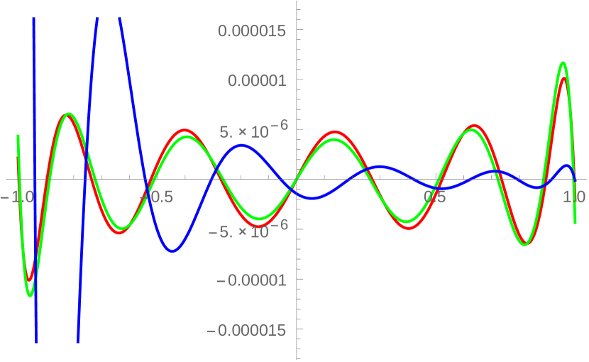
Figure 1: $N=30,m=10$, approximation error, parameters: $(0,0)$ (red), $(0.5,0.5)$ (green), $(5,0)$ (blue)

We recognize that for all parameter selections the pointwise error is very small and the truncated series expansions describe the function $f$ fairly good. This fact is also reflected in the coefficients $\hat{f}_{n}$ the absolute values of which are shown in Figure 2.

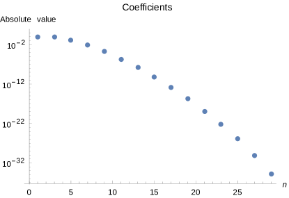
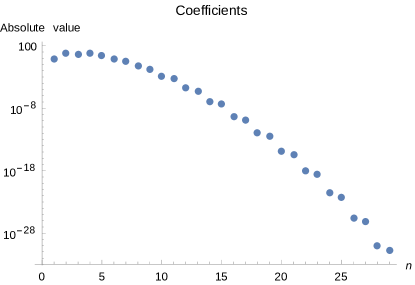
Figure 2: Absolute values of the coefficients $\hat{f}_{n}$

On the left hand side the Hahn polynomials with the parameters $(0,0)$ are used and on the right-hand side $(5,0)$. We realize an exponential decay in logarithmic scale in both figures. Furthermore, for $(0,0)$ the odd coefficients only appear. All even coefficients are zero and have no influence on the approximation. Because of the symmetry of the sine function and the special choice of the parameters $(\alpha,\beta)=(0,0)$ this is not suprising. We see this same effect in the Legendre coefficients, where all even coefficients are zero, as can be seen in figure 4. Another interesting fact is the approximation speed being faster by using Hahn polynomials, compare figures 4 and 2.

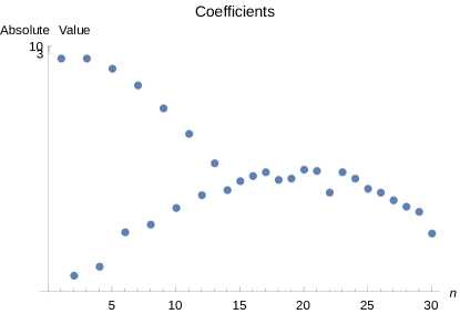
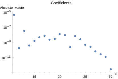
Figure 3: Absolute values of the coefficients $\hat{f}_{n}$

Figure 3 demonstrates the absolute values of the coefficients in the case $(0.5,0.5)$. Taking a closer look on the behaviour of the coefficients, we see that the even coefficients do not play a major role in the approximiaton, but their influence rises with growing $n$ and their absolute value increases. The value of the even and odd coefficients is nearly the same around $n=14/15$ and remain up to $n=23$ at this level which is between $[10^{-10},10^{-8}]$. This circumstances can be explained by the fact that the Hahn polynomials of even degree like, $Q_{2n}(x,\alpha,\beta,N)$, have odd parts. When $n$ increases also these parts grow and their influence grows. However, in the end we again get spectral accuracy in the coefficients, what was predicted in Theorem 3.1.

Remark 4.1.

We note that this special behaviour of the rising influence of the even coefficients is characteristic for using Hahn polynomials with parameters $\alpha,\beta\notin\mathbb{N}_{0}$ in approximating the odd sine function. A comparable result can be seen if approximating an even function. Then the influence of the odd coefficients rises at the beginning.

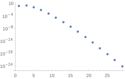
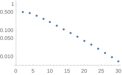
Figure 4: Absolute values of the coefficients for $\hat{f}_{n}$ and $\hat{g}_{n}$ using Legendre polynomials

In the second example we consider the function $g(x)=\frac{1}{1+25x^{2}}$ on the intervall $I=[-1,1]$. The absolute value of the Hahn coefficients are plotted in a logarithmic scale. We use $N=30$ and the parameters $(\alpha,\beta)=(0,0),\;(5,0)$ and $(0.5,0.5)$.

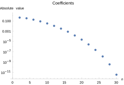
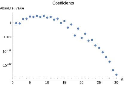
Figure 5: Absolute values of the coefficients $\hat{g}_{n}$, parameters $(0,0)$ and $(5,0)$

In figures 5 and 6 we see the coefficients $\hat{g}_{n}$ as functions of the degree $n$. We recognize a behaviour, which we have already noticed in the first example. In the case of the parameters $(\alpha,\beta)=(0,0)$ all odd coefficients are zero and only the even coefficients are needed in the approximation. In case of $(0.5,0.5)$ the absolute value of the odd coefficients increases due to the fact that the Hahn polynomials of odd degree have an even part, and this part grows in $n$.

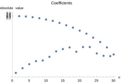
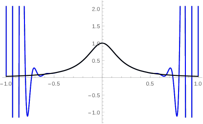
Figure 6: Absolute values of the coefficients $\hat{g}_{n}$ parameters $(0.5,0.5)$, Runge phenomenon

In all cases we see spectral accuracy in the coefficients even though the absolute values increase in the beginning in the case $(5,0)$. Simultaneously we do not get the same level as in the sine example and also we get a further problem. It is well-known that approximating the function $g$ with the usual interpolation polynoms on an equidistant grid yields the Runge phenomenon. If we approximate with $m=30$ our truncated Hahn series becomes the usual interpolation polynomial on equidistant points and we also obtain the Runge phenomenon, see figure 6, where the black line marks the original function $g$. In figure 7 we plot the truncated Hahn series with $m=10$ for the parameters $(\alpha,\beta)=(0,0)$ (red), $(0.5,0.5)$ (green), ($5,0)$ (blue). In the right figure we demonstrate the pointwise approximation error. We conclude that all truncated series expansions do not describe the original function and the quality of the approximation also depends on the parameter selection $\alpha,\beta$. The Runge phenomenon has an influence on the approximation and we have to take this fact into consideration.

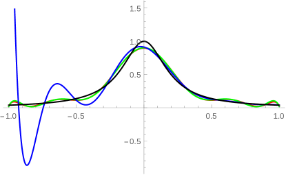
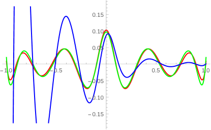
Figure 7: Truncated series with $m=10$, approximation error

5 Discussion and an outlook

Applying the Hahn polynomials in a spectral method for the numerical solution of conservation laws we will not commit any numerical calculation errors by using the projection approach, but we may have also to deal with the Runge phenomenon. We can not ensure that our approximated solution really describes the correct one and the question is now: How can we fix this problem?
In [6] the authors use discrete orthogonal polynomials for approximation and solving differential equations. Their basic idea is to split the domain and to approximate not on equidistant points near the boundary, instead they use Chebyshev nodes to avoid the Runge phenomenon.

In [4] the authors construct discrete orthogonal polynomials via a quadrature rule from Chebyshev nodes up to a particular, but fixed degree. These are not classical discrete orthogonal polynomials and therefore some basic properties do not exist or are not known like the satisfaction of an eigenvalue equation. Nevertheless one should analyse their approximation properties and also apply them in a numerical method to solve differential equations. We will consider this in a further paper.
Here our focus was on the Hahn polynomials and their approximation properties, because they have all the basic properties which we will need later to construct a discrete filter. Furthermore we can extend these polynomials similar to the Jacobi polynomials in the continuous case to triangular meshes. Many numerical methods use triangulations to split the domain into different elements. In the area of computational fluid dynamics triangular grids are optimal for the description of complex geometries. This is one reason why we are interested in an extension of the Hahn polynomials on triangles, and this was already done by Xu, see [26, 27].
First of all, we have to deal with the problem of the Runge phenomenon, when using the truncated Hahn series. Therefore, we have to understand the approximation properties of the series and the pointwise error in particular. We already started to investigate the behaviour of the pointwise truncation error in [9] and estimated the pointwise error of the truncated Hahn series with respect to the pointwise error of the truncated Jacobi series. The occurrence of the Runge phenomenon is already studied in-depth, see [24], but nevertheless, we are also looking for additional and further conditions on the function $u$ to ensure that the Runge phenomenon has no influence on the approximation.
The last idea is motivated by the Gegenbauer reconstruction in [10, 11]. The basic idea of the Gegenbauer reconstruction is to develop the numerical solution once more in a series expansion to delete the Gibbs’ phenomenom. The authors investigate the ratio between the order $m$ of the Gegenbauer polynomials and the truncation index $N$ of the series. They prove some convergence results, for details see [10]. In [1] the author showed that singularities off the real axis can destroy convergence if $m,N$ tend simultaneously to infinity. The Gegenbauer reconstruction must therefore be constrained to use a sufficiently small ratio of order $m$ to truncation $N$. In [5] the reconstruction procedure is further investigated using another orthogonal basis of the Freud polynomials. We will transfer their ideas to our problem and will analyse the ratio between the $N$ Hahn polynomials and truncation $m$, which are finally used in the series expansion, to minimize the total error.

6 Appendix:

Let $s,r\in\mathbb{N}$. The hypergeometric function ${}_{r}F_{s}$ is defined by the series

$${}_{r}F_{s}\left(a_{1},\cdots,a_{r};b_{1},\cdots b_{s};z\right)\mathrel{\mathop{\ordinarycolon}}=\sum\limits_{k=0}^{\infty}\frac{(a_{1},\cdots,a_{r})_{k}}{(b_{1},\cdots,b_{s})_{k}}\frac{z^{k}}{k!},$$ (11)

where

$$(a_{1}\cdots,a_{r})_{k}\mathrel{\mathop{\ordinarycolon}}=(a_{1})_{k}\cdots(a_{r})_{k}.$$

The parameters must be such that the denominator factors in the terms of the series are never zero. When one of the numerator parameters $a_{i}$ equals $-n$, where $n$ is a nonnegative integer, this hypergeometric function is a polynomial in $z$.

References

- [1] J. P. Boyd. Trouble with gegenbauer reconstruction for defeating gibbs’ phenomenon: Runge phenomenon in the diagonal limit of gegenbauer polynomial approximations. J. of Computational Physics, (204):253–264, 2005.
- [2] P. Butzer and F. Jongmans. P. L. Chebyshev (1821–1894). A guide to his life and work. J. Approx. Theory, 96(1):111–138, 1999.
- [3] C. Canuto, M. Y. Hussaini, A. Quarteroni, and T. A. Zang. Spectral methods in fluid dynamics. Springer Series in Computational Physics. Springer-Verlag, New York, 1988.
- [4] A. Eisinberg and G. Fedele. Discrete orthogonal polynomials on Gauss-Lobatto Chebyshev nodes. J. Approx. Theory, 144(2):238–246, 2007.
- [5] A. Gelb. Reconstruction of piecewise smooth functions from non-uniform grid point data. J. Sci. Comput., 30(3):409–440, 2007.
- [6] A. Gelb, R. B. Platte, and W. St. Rosenthal. The discrete orthogonal polynomial least squares method for approximation and solving partial differential equations. Commun. Comput. Phys., 3(3):734–758, 2008.
- [7] Jan Glaubitz, Philipp Öffner, and Thomas Sonar. Application of modal filtering to a spectral difference method, 2016. Submitted.
- [8] Jan Glaubitz, Hendrik Ranocha, Philipp Öffner, and Thomas Sonar. Enhancing stability of correction procedure via reconstruction using summation-by-parts operators II: Modal filtering, 2016. Submitted.
- [9] R. Goertz and P. Öffner. On Hahn polynomial expansion of a continuous function fo bounded variation. 2016. Submitted.
- [10] D. Gottlieb and C.-W. Shu. On the Gibbs phenomenon and its resolution. SIAM Rev., 39(4):644–668, 1997.
- [11] David Gottlieb, Chi-Wang Shu, Alex Solomonoff, and Hervé Vandeven. On the gibbs phenomenon i: recovering exponential accuracy from the fourier partial sum of a nonperiodic analytic function. Journal of Computational and Applied Mathematics, 43(1):81 – 98, 1992.
- [12] HT Huynh. A flux reconstruction approach to high-order schemes including discontinuous Galerkin methods. AIAA paper, 4079:2007, 2007.
- [13] HT Huynh, Zhi J Wang, and Peter E Vincent. High-order methods for computational fluid dynamics: A brief review of compact differential formulations on unstructured grids. Computers & Fluids, 98:209–220, 2014.
- [14] G. E. Karniadakis and S. J. Sherwin. Spectral/ element methods for computational fluid dynamics. Numerical Mathematics and Scientific Computation. Oxford University Press, New York, second edition, 2005.
- [15] R. Koekoek, P. A. Lesky, and R. F. Swarttouw. Hypergeometric orthogonal polynomials and their -analogues. Springer Monographs in Mathematics. Springer-Verlag, Berlin, 2010. With a foreword by Tom H. Koornwinder.
- [16] A. Meister, S. Ortleb, T. Sonar, and M. Wirz. A comparison of the discontinuous-Galerkin- and spectral-difference-method on triangulations using PKD polynomials. J. Comput. Phys., 231(23), 2012.
- [17] A. Meister, S. Ortleb, T. Sonar, and M. Wirz. An extended discontinuous Galerkin and spectral difference method with modal filtering. ZAMM Z. Angew. Math. Mech., 93(6-7):459–464, 2013.
- [18] A. F. Nikiforov, S. K. Suslov, and V. B. Uvarov. Classical orthogonal polynomials of a discrete variable. Springer Series in Computational Physics. Springer-Verlag, Berlin, 1991. Translated from the Russian.
- [19] P. Öffner and T. Sonar. Spectral convergence for orthogonal polynomials on triangles. Numer. Math., 124(4):701–721, 2013.
- [20] F. Olver, D. Lozier, Roland B., and Ch. Clark, editors. NIST Handbook of Mathematical Functions. Cambridge University Press, New York, NY, 2010. Printed version of [22].
- [21] Hendrik Ranocha, Philipp Öffner, and Thomas Sonar. Summation-by-parts operators for correction procedure via reconstruction. Journal of Computational Physics, 311:299–328, 2016.
- [22] Nist digital library of mathematical functions. ”http://dlmf.nist.gov/, Release 1.0.9 of 2014-08-29”. Online Conclusion of [20].
- [23] Ch. Schwab. - and -finite element methods. Numerical Mathematics and Scientific Computation. The Clarendon Press, Oxford University Press, New York, 1998. Theory and applications in solid and fluid mechanics.
- [24] Lloyd N Trefethen. Approximation theory and approximation practice. Siam, 2013.
- [25] ZJ Wang and Haiyang Gao. A unifying lifting collocation penalty formulation including the discontinuous Galerkin, spectral volume/difference methods for conservation laws on mixed grids. Journal of Computational Physics, 228(21):8161–8186, 2009.
- [26] Y. Xu. On discrete orthogonal polynomials of several variables. Advances in Applied Mathematics, 33(3):615–631, 2004.
- [27] Y. Xu. Second-order difference equations and discrete orthogonal polynomials of two variables. Int. Math. Res. Not., (8):449–475, 2005.