Evolution of CO₂, CH₄, and OCS abundances relative to H₂O in the coma of comet 67P around perihelion from Rosetta/VIRTIS-H observations

Abstract

Infrared observations of the coma of 67P/Churyumov-Gerasimenko were carried out from July to September 2015, i.e., around perihelion (13 August 2015), with the high-resolution channel of the VIRTIS instrument onboard Rosetta. We present the analysis of fluorescence emission lines of H₂O, CO₂, ¹³CO₂, OCS, and CH₄ detected in limb sounding with the field of view at 2.7–5 km from the comet centre. Measurements are sampling outgassing from the illuminated southern hemisphere, as revealed by H₂O and CO₂ raster maps, which show anisotropic distributions, aligned along the projected rotation axis. An abrupt increase of water production is observed six days after perihelion. In the mean time, CO₂, CH₄, and OCS abundances relative to water increased by a factor of 2 to reach mean values of 32 %, 0.47 %, and 0.18%, respectively, averaging post-perihelion data. We interpret these changes as resulting from the erosion of volatile-poor surface layers. Sustained dust ablation due to the sublimation of water ice maintained volatile-rich layers near the surface until at least the end of the considered period, as expected for low thermal inertia surface layers. The large abundance measured for CO₂ should be representative of the 67P nucleus original composition, and indicates that 67P is a CO₂-rich comet. Comparison with abundance ratios measured in the northern hemisphere shows that seasons play an important role in comet outgassing. The low CO₂/H₂O values measured above the illuminated northern hemisphere are not original, but the result of the devolatilization of the uppermost layers.

1 Introduction

Comets are among the most pristine objects of the Solar System. The chemical composition of nucleus ices should provide insights for the conditions of formation and evolution of the early Solar System. A large numbers of molecules have now been identified in cometary atmospheres, both from ground-based observations and space, including in situ investigations of cometary atmospheres (Bockelée-Morvan et al., 2004; Cochran et al., 2015; Le Roy et al., 2015; Biver et al., 2015a; Biver & Bockelée-Morvan, 2016). Molecular abundances relative to water present strong variations from comet to comet, and also vary along comet orbit (e.g., Biver & Bockelée-Morvan, 2016; Ootsubo et al., 2012; McKay et al., 2015, 2016). This chemical diversity is often interpreted as reflecting different formation conditions in the primitive solar nebula (e.g., A’Hearn et al., 2012). However, questions arise concerning the extent to which abundances measured in cometary atmospheres are representative of the pristine composition of nucleus ices. Models investigating the thermal evolution and outgassing of cometary nuclei show that the outgassing profiles of cometary molecules depend on numerous factors such as molecule volatility, thermal inertia of the nucleus material, nature of water ice structure, and dust mantling (De Sanctis, Capria, & Coradini, 2005; De Sanctis, Lasue, & Capria, 2010a; De Sanctis et al., 2010b; Marboeuf & Schmitt, 2014).

The study of the development of cometary activity, with the goal to relate coma and nucleus chemical properties, is one of the main objectives of the Rosetta mission of the European Space Agency (Schulz, 2012). Rosetta reached comet 67P/Churyumov-Gerasimenko (hereafter referred to as 67P) in August 2014 at $r_{h}$ = 3.5 AU from the Sun, and accompanied it in its journey towards perihelion (13 August 2015, $r_{h}$ = 1.24 AU), with the end of the mission in September 2016. The scientific instruments on the orbiter and Philae lander provided complementary information on the physical and chemical properties of the nucleus surface and subsurface, and of the inner coma. They revealed a dark, organic-rich and low-density bi-lobed nucleus with a morphologically complex surface showing different geological terrains, some of them with smooth dust-covered areas (Sierks et al., 2015; Capaccioni et al., 2015; Pätzold et al., 2016). Dust jets originating from active cliffs, fractures and pits were observed (Vincent et al., 2016). Water vapour was first detected in June 2014, at 3.93 AU from the Sun (Gulkis, 2014; Gulkis et al., 2015). In data obtained pre-equinox (May 2015), the water outgassing was found to correlate well with solar illumination, though with a large excess from the brighter and bluer Hapi region situated in the northern hemisphere (Biver et al., 2015b; Bockelée-Morvan et al., 2015; Feldman et al., 2015; Migliorini et al., 2016; Fink et al., 2016; Fougere et al., 2016a). In the Hapi active region, VIRTIS has observed that surficial water ice has diurnal variability showing sublimation and condensation cycle occurring with the change of illumination conditions (De Sanctis et al., 2015). In contrast, CO₂ originated mainly from the poorly illuminated southern hemisphere (Hässig et al., 2015; Migliorini et al., 2016; Fink et al., 2016; Fougere et al., 2016a), where VIRTIS identified a CO₂ ice-rich area (specifically in the Anhur region Filacchione et al., 2016a).

The large obliquity (52^∘) of the 67P rotation axis (Sierks et al., 2015) leads to strong seasonal effects on its nucleus, with the northern regions experiencing a long summer at large distances from the Sun whereas the southern polar regions are subject to a short-lived, but extremely intense summer season around perihelion. In this paper, we present observations of H₂O, CO₂, ¹³CO₂, OCS, and CH₄ in the vapour phase undertaken with the high spectral resolution channel of the Visible InfraRed Thermal Imaging Spectrometer (VIRTIS) (Coradini et al., 2007) near perihelion (early July to end of September 2015). The paper is organized as follow: Section 2 presents the VIRTIS-H instrument, the data set and raster maps of H₂O and CO₂ which provide the context for the off-limb observations studied in the paper; in Sect. 3, we present the detected molecular emission lines and the fluorescence models used for their analysis; section 4 presents the data analysis and the column densities measured for H₂O, CO₂, CH₄, and OCS, and their relative abundances; an interpretation of the results and a discussion follows in Sect. 5.

2 Observations

2.1 VIRTIS-H instrument

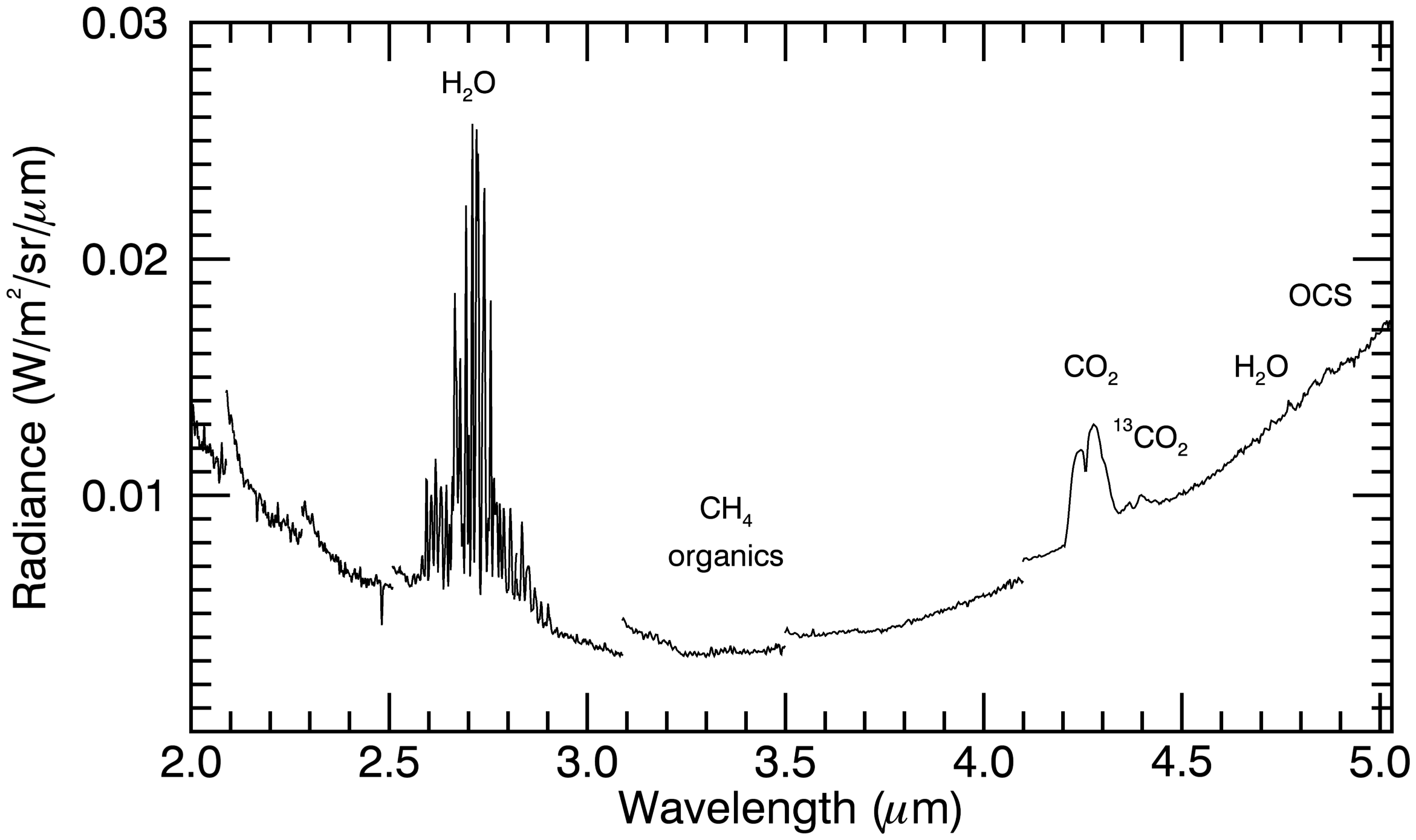
Figure 1: Full VIRTIS-H spectrum obtained by averaging the 3 data cubes obtained on 19 Aug. 2015. At this scale, the faint emissions from CH₄, OCS and H₂O 4.5–5 $\mu$m bands are not easily distinguishable. The short wavelength range of the spectral orders is contaminated by instrumental straylight (e.g., at 2.1 and 2.28 $\mu$m), resulting in a higher radiance.

The VIRTIS instrument is composed of two channels: VIRTIS-M, a spectro-imager operating both in the visible (0.25–1 $\mu$m) and infrared (1–5 $\mu$m) ranges at moderate spectral resolution ($\lambda$/$\Delta\lambda$ = 70-380), and VIRTIS-H, a point spectrometer in the infrared (1.9–5.0 $\mu$m) with higher spectral resolution capabilities (Coradini et al., 2007). The infrared channel of VIRTIS-M stopped providing cometary data in May 2015, due to a cryocooler failure. Only VIRTIS-H data are used in this paper.

VIRTIS-H is a cross-dispersing spectrometer consisting of a telescope, an entrance slit, followed by a collimator, and a prism separating eight orders of a grating (Drossart et al., 2000; Coradini et al., 2007). The spectra investigated in this paper are in orders 0 (4.049–5.032 $\mu$m) and 2 (3.044–3.774 $\mu$m). Each order covers 432 $\times$ 5 pixels on the detector. A "pixel map" locates the illuminated pixels. The field of view corresponds to a 5-pixel wide area on the focal plane array; in nominal mode (most data), the summation of the signals received on these pixels (actually only the 3 more intense) is performed on-board. The spectra are therefore sampled by 3456 spectral elements, 432 in each grating order. As for most Rosetta instruments, the line of sight of VIRTIS is along the Z-axis of the spacecraft (S/C). The instantaneous field of view (FOV) of the VIRTIS-H instrument is 0.58 $\times$ 1.74 mrad² (the larger dimension being along the Y axis).

The VIRTIS-H data are processed using the so-called CALIBROS pipeline. This pipeline subtracts dark current, corrects for the instrumental function (odd/even pixels effects, de-spiking), and calibrates the absolute flux of the spectra in radiance (W/m²/sr/$\mu$m). Stray light is present in some spectra on the short-wavelength side of each order, depending on the location of the nucleus with respect to the slit (Fig 1).

The nominal numerical spectral resolving power $\lambda$/$\Delta\lambda$ varies between 1300 and 3500 within each order, where $\Delta\lambda$ is the grating resolution. The spectral sampling interval is 1.2–1.3 $\Delta\lambda$, and thus above Nyquist sampling. In the current calibration, odd/even effects were overcome by performing spectral smoothing with a boxcar average over 3 spectral channels, thereby reducing the effective spectral resolution to a value $\sim$ 2.7 $\times$ $\Delta\lambda$, which was experimentally verified by fitting spectra of the H₂O and CO₂ bands in order 4 and 0, respectively (Debout, 2015). The effective spectral resolution with the current calibration is $\sim$ 800 at 3.3 and 4.7 $\mu$m.

The geometric parameters of the observations have been computed using nucleus shape model SHAP5 v1.1, derived from OSIRIS images (Jorda et al., 2016).

2.2 Data set

Table 1: Log of VIRTIS-H observations.

Obs Id	Start time	Duration	Date wrt	$r_{h}$	$\Delta$(S/C)	phase	Pointinga		South poleb
			perihelion				$\rho$	$PA$	$PA$	Aspect
	(UT)	(hr)	(d)	(AU)	(km)	(∘)	(km)	(∘)	(∘)	(∘)
00395011055	2015-07-08T21:11:00.3	3.51	-35.2	1.316	150	90	2.82	259	328	108
00395322550	2015-07-12T11:46:52.6	3.66	-31.6	1.302	153	89	2.70	274	327	101
00395742154	2015-07-17T08:15:55.9	2.56	-26.7	1.286	177	90	3.10	272	302	137
00396199623	2015-07-22T15:23:57.9	4.27	-21.4	1.271	169	89	2.69	266	319	110
00396220410	2015-07-22T21:10:24.7	3.60	-21.2	1.270	170	89	2.98	266	319	109
00396659230	2015-07-27T23:06:40.5	3.54	-16.1	1.259	177	90	4.01	247	311	60
00396826054	2015-07-29T21:20:59.8	3.24	-14.2	1.255	179	90	3.56	265	286	44
00396842044	2015-07-30T01:47:25.8	3.91	-14.0	1.255	177	90	3.59	265	281	43
00397038715	2015-08-01T08:25:16.8	0.67	-11.7	1.252	214	90	3.08	270	238	52
00397871165	2015-08-10T23:32:29.0	2.80	-2.1	1.244	323	89	6.23	286	242	123
00398347798	2015-08-16T11:56:25.1	3.31	3.4	1.244	327	89	3.58	267	288	127
00398603680	2015-08-19T11:08:06.5	3.24	6.4	1.246	329	90	2.96	263	302	115
00398619671	2015-08-19T15:34:33.4	3.91	6.6	1.246	327	90	2.97	262	303	114
00398640452	2015-08-19T21:20:58.5	3.24	6.8	1.246	326	90	3.47	262	304	112
00398729980	2015-08-20T22:13:06.6	3.91	7.8	1.247	325	90	4.58	258	307	105
00398970868	2015-08-23T17:07:54.5	3.10	10.6	1.250	340	87	3.78	256	309	80
00398986563	2015-08-23T21:29:29.5	3.78	10.8	1.251	343	87	3.82	255	308	78
00399198695	2015-08-26T08:17:52.6	1.02	13.3	1.254	414	83	4.25	264	302	59
00399208316	2015-08-26T10:58:13.4	3.56	13.4	1.254	410	83	3.95	263	301	57
00400195914	2015-09-06T21:25:16.9	3.91	24.8	1.280	339	108	4.92	266c	231	124
00400216374	2015-09-07T03:06:16.9	3.24	25.0	1.281	332	110	4.87	268c	231	127
00400232094	2015-09-07T07:28:16.8	3.91	25.2	1.282	327	111	4.83	268c	232	131
00400252549	2015-09-07T13:09:16.0	3.24	25.5	1.282	322	112	4.83	270c	232	134
00400407713	2015-09-09T08:15:16.0	1.08	27.3	1.288	331	119	3.14	263	255	156
00400433767	2015-09-09T15:29:34.0	4.05	27.6	1.289	324	120	3.72	262	263	157
00400470243	2015-09-10T01:37:26.0	4.18	28.0	1.290	318	120	5.78	263d	274	158
00400748481	2015-09-13T06:54:44.2	3.51	31.2	1.301	313	110	3.58	265	307	132
00400765976	2015-09-13T11:46:19.3	3.64	31.4	1.302	312	108	3.61	265	307	129
00401717336	2015-09-24T11:55:21.0	4.07	42.4	1.347	488	63	5.02	275	317	60
00401994267	2015-09-27T16:57:54.5	3.51	45.6	1.362	1057	51	6.88	282	329	35

^a Except when indicated, the FOV is staring at a fixed distance $\rho$ from the comet centre at the given position angle $PA$ which is close to the Sun direction ($PA$(Sun) = 270^∘).

^b Orientation of South Pole direction defined by its position angle in the plane of the sky and its aspect angle with respect to the line of sight.

^c The S/C was continuously slewing along the $Y$ axis, i.e., perpendicularly to the comet-Sun line providing data at $y$=–4 to + 4 km with $x$ fixed; $PA$ was ranging from 220–310^∘, only the mean $PA$ is indicated.

^d Two stared positions were commanded, whereas we used the closest to comet center.

The data set was selected with the objective of studying spectral signatures of a number of species and derive their relative abundances. As presented in the next sections (see Fig. 1), five molecules (H₂O, CO₂, ¹³CO₂, OCS, and CH₄) are detected unambiguously around perihelion (on 13.0908 August UT), not considering organic molecules contributing to the 3.4 $\mu$m band. Whereas H₂O and CO₂ present strong signatures at 2.7 and 4.3 $\mu$m, respectively, which were detected by VIRTIS-H starting October 2014 (Bockelée-Morvan et al., 2015), these bands became optically thick around perihelion time. Hence, in this paper we consider the July to September 2015 period during which optically thin H₂O and CO₂ hot-bands, and ¹³CO₂ are detected. An appropriate radiative transfer analysis (following, e.g., Debout, Bockelée-Morvan, & Zakharov, 2016) of the optically thick H₂O and CO₂ bands will be presented in forthcoming papers. Specifically, we analysed the $\nu_{3}$-$\nu_{2}$ and $\nu_{1}$–$\nu_{2}$ H₂O hot bands falling in the 4.4–4.5 $\mu$m range, and the CO₂ $\nu_{1}$+$\nu_{3}$–$\nu_{1}$ bands at 4.3 $\mu$m.

Coma observations with VIRTIS-H were performed in various pointing modes, e.g., stared pointing at a fixed limb distance in inertial frame or raster maps. In this paper, we consider mostly those with the FOV staring at a distance of less than 5 km from the comet surface (distance from comet center less than 7 km) along the projected comet-Sun line. These observations are those providing the largest signal-to-noise ratios in the spectra. In addition, we considered four data cubes with acquisitions scanning a line of 8-km long perpendicular to the Sun direction and above the illuminated nucleus (data of 6–7 September 2015, Table 1). The mean distances to the comet center ($\rho$) for the considered data cubes are between 2.7 and 6.9 km (Table 1).

Altogether thirty data cubes, lasting typically 3–4 h each, were selected. They are listed in Table 1, together with geometric parameters (phase angle, heliocentric distance $r_{h}$, and distance of the S/C to the comet, mean distance of the FOV with respect to the comet center and position angle). For these observations, the acquisition time is 3 s, except for the July 12th and 27th observations for which it is 1 s, and the dark rate is 4 (one dark image every 4 acquisitions). Frame summing has been performed on-board for data volume considerations, e.g., by summing pair of acquisitions. The total number of acquisitions in the data files is between 256 (case of first Aug. 26th observation) and 7424 (observation of July 27th).

For most of the selected observations the S/C was in the terminator plane (phase angle $\sim$ 90^∘). Therefore these observations were favourable for sampling molecules outgassed from the illuminated regions of the nucleus. However, the two last data cubes were acquired with a smaller phase angle $\sim$ 50–60^∘, with the closest points to the line of sight (LOS) situated from less illuminated regions, so that less intense signals are expected (and indeed observed). During the period, the Rosetta spacecraft was at distances from the comet from 150 to 480 km (with the exception of the 27 September observation with the S/C at 1057 km, Table 1). The VIRTIS-H FOV then ranged from 90 $\times$ 260 m to 280 $\times$ 850 m in the orthogonal plane containing the comet, which can be compared to the typical size of 67P nucleus of 2 km equivalent radius. This means that molecules detected in the field of view are potentially originating from a broad range of longitudes and latitudes.

2.3 Context VIRTIS-H raster maps

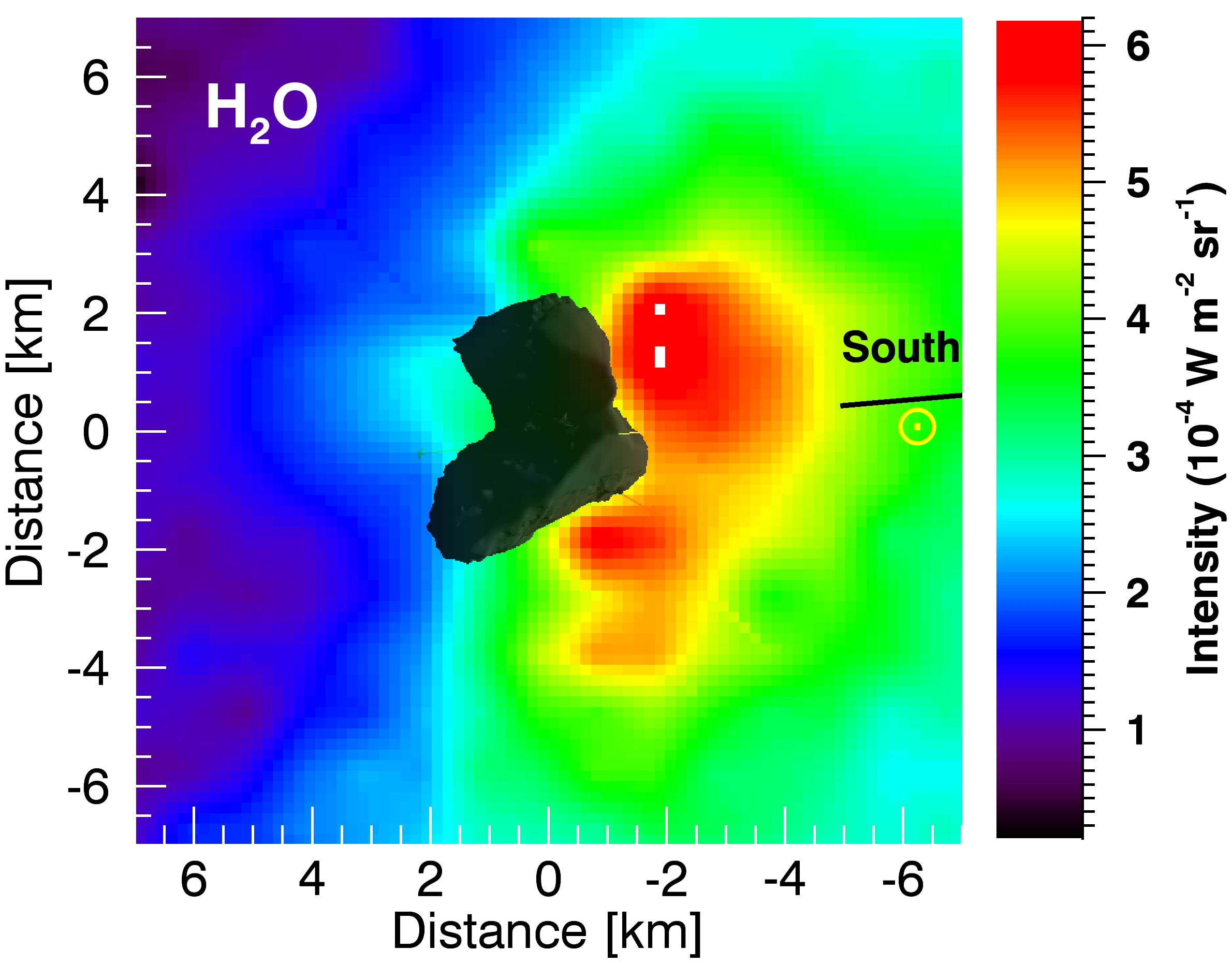
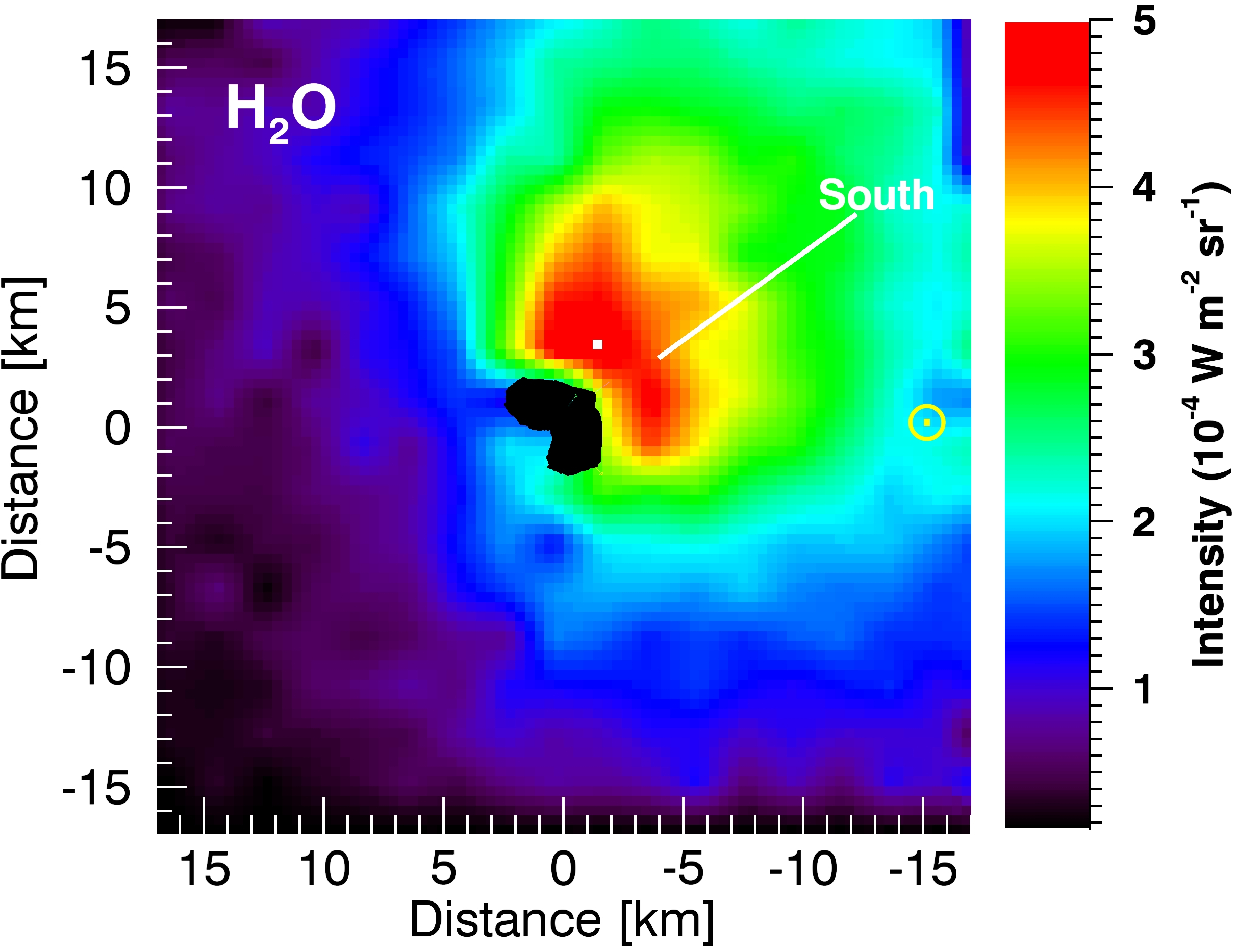
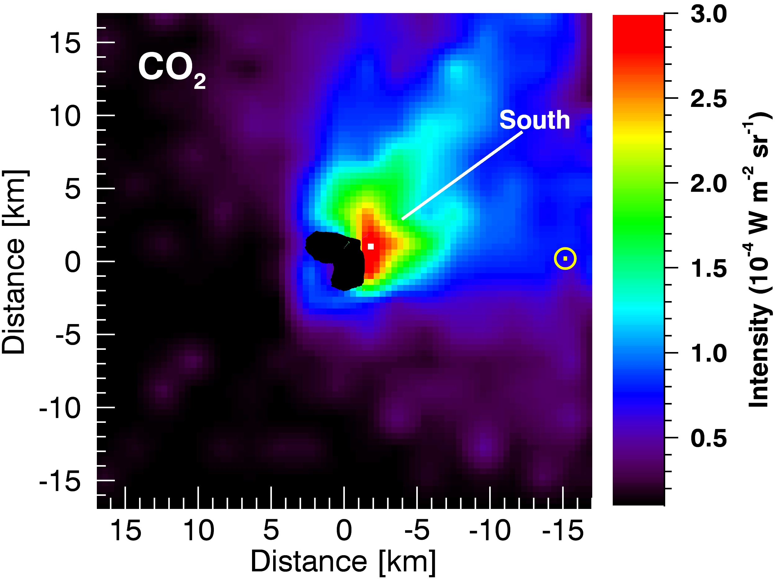
Figure 2: VIRTIS-H raster maps of the H₂O 2.7 and CO₂ 4.3 $\mu$m bands. Top: H₂O on 30 July 2015, 19h:25 UT (ObsId: 00396898661). Middle and bottom: H₂O and CO₂, respectively, on 9 August 2015, 3h:10 UT (ObsId: 00397703949). The projection of the rotation axis (South direction) and Sun direction are indicated. The observational parameters are: line spacing of 0.6 km and 2 km, slew rate of 1.0 and 1.75 deg/min, for 30 July and 9 August, respectively. The maps were obtained after averaging spectra within cells of sizes of 1 km (30 July) and 2 km (9 August).

As a result of the  52^∘ obliquity and the orientation of the 67P rotation axis (Sierks et al., 2015), the perihelion period corresponds to the time where only the southern regions are illuminated. During the July-September period, the sub-solar latitude varied between –26 ^∘ to –52^∘, with the lowest value reached on 4 September 2015.

In order to put the limb observations analysed in this paper into context, we show in Fig. 2 VIRTIS-H raster maps of the H₂O 2.7 $\mu$m and CO₂ 4.3 $\mu$m bands obtained on 30 July and 9 August 2015, when Rosetta was at 181 km and 303 km from the comet, respectively. These maps (not listed in Table 1) were obtained by slewing the spacecraft along the $X$ S/C axis (with the Sun being in the -$X$ direction), setting a line spacing in the $Y$ direction. The observation duration is 3–4 h, i.e., 1/4 to 1/3 of the rotation period of $\sim$ 12 h (Sierks et al., 2015), so there is some smearing related to nucleus rotation. Spatial binning was applied, by averaging spectra into cells of size of 1 and 2 km. After baseline removal, the CO₂ band area was determined by gaussian fitting, whereas that of the H₂O band by summing the radiances measured in the wavelength interval 2.6–2.73 $\mu$m.

The distributions of the H₂O and CO₂ band intensities display a fan-shaped morphology aligned along the South direction of the rotation axis (Fig. 2), indicating that these molecules were mainly released from the southern regions. Because the Rosetta S/C was moving around the comet, the position angle $PA$ of the rotation axis in the ($X$, $Y$) S/C frame changed with time, spanning value between 240 and 330^∘ in the July-November timeframe (Table 1), with the Sun at +270^∘ in the adopted $PA$ definition ($PA$ = 0 for the +$Y$ axis, $PA$ = 90^∘ for +$X$). VIRTIS-H maps acquired from August to November 2015 in different $PA$ configurations all show a tight correlation between the orientation of the H₂O and CO₂ fans and the North-South line (Bockelée-Morvan et al., 2016). This is consistent with in situ data obtained by the Rosetta Orbiter Spectrometer for Ion and Neutral Analysis (ROSINA) (Fougere et al., 2016b).

As regards the stared off-limb observations considered in this paper, they probe coma regions at $PA$ close to the projected comet-Sun line. The PA of the FOV is given for each data cube in Table 1. The angle between the PA of the FOV and the main fan direction is the range 0–70^∘ (with 70% of the observations with an offset less than 45^∘). Since the angular width of the H₂O and CO₂ fans was measured to be typically 110^∘ and 180^∘ for H₂O and CO₂, respectively (Bockelée-Morvan et al., 2016), coma regions within the molecular fan were observed most of the time.

3 Observed fluorescence emissions and modelling

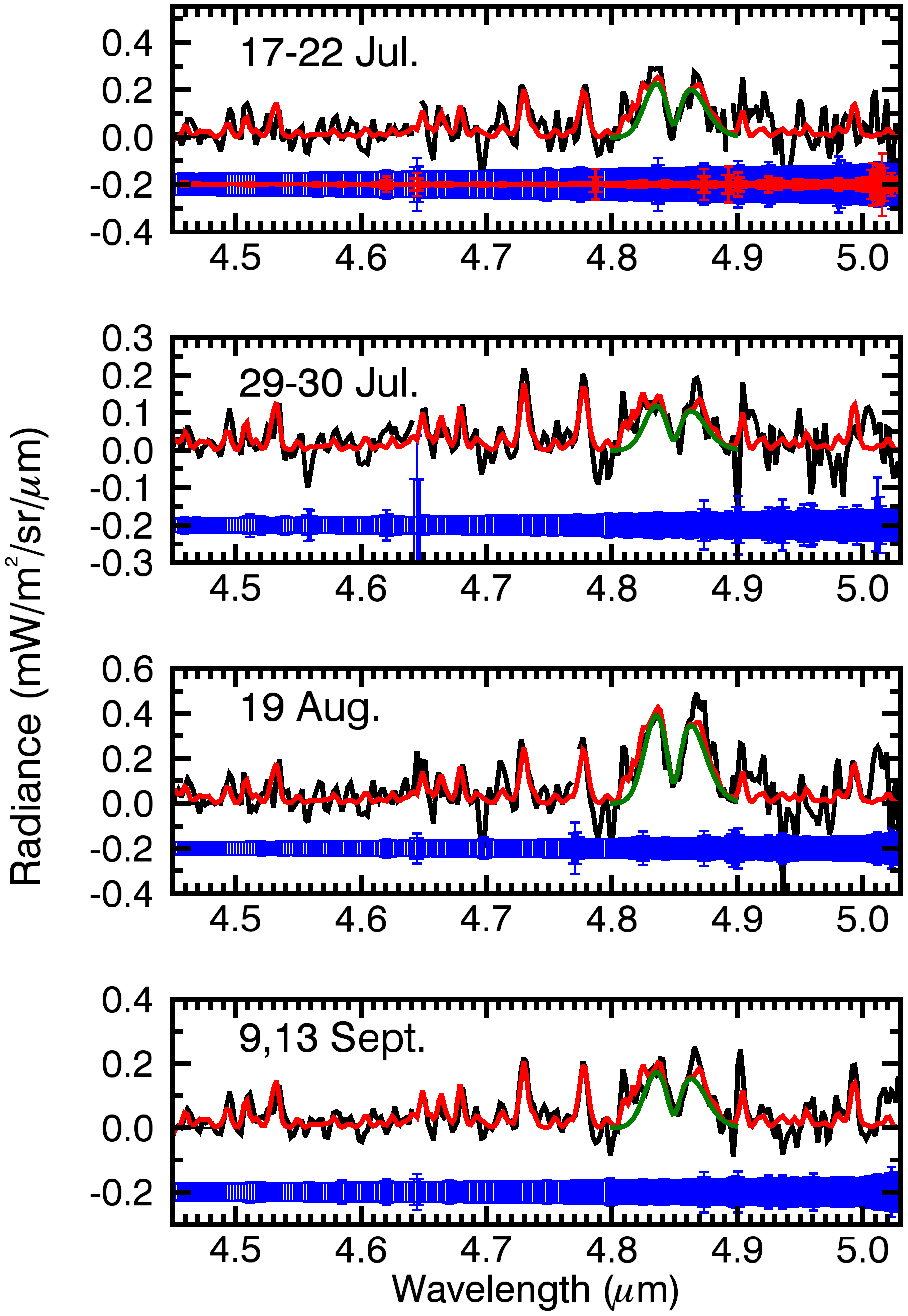
Figure 3: VIRTIS-H spectra in the range 4.45–5 $\mu$m showing ro-vibrational lines of the H₂O $\nu_{3}-\nu_{2}$ band, and the OCS $\nu_{3}$ band. The red line displays the fitted synthetic spectrum for a temperature of 120 K, including both H₂O and OCS. The green line shows the contribution due to OCS only. A: 17–22 July; B : 29–30 July; C: 19 Aug.; D: 9, 13 Sept. The standard deviation for each spectral channel is shown in the bottom of the plots (for better reading, the errorbars are offsetted with respect to the measured radiances); values in blue include time variations in the continuum. In the top plot, the standard deviation measured on a spectrum with no comet signal (and scaled to the observing time of the comet spectrum) is superimposed, in red.

3.1 H₂O

H₂O is detected both in the 2.5–2.9 $\mu$m (covered by orders 3, 4 and 5 of the spectrograph) and in the 4.45–5.0 $\mu$m range (order 0) (Figs 1-3). The ro-vibrational lines detected in the 2.5–2.9 $\mu$m region are from the $\nu_{3}$ and $\nu_{1}$ fundamental bands, and from several hot bands ($\nu_{1}$+$\nu_{3}$–$\nu_{1}$, $\nu_{2}$+$\nu_{3}$–$\nu_{2}$, and the weaker $\nu_{1}$+$\nu_{3}$–$\nu_{3}$ band, Bockelée-Morvan & Crovisier (1989); Villanueva et al. (2012)). With the spectral resolution of the data, the ro-vibrational structure of these bands is partially resolved. The intensity of the $\nu_{3}$ band is expected to be significantly affected by optical depth effects (Debout, Bockelée-Morvan, & Zakharov, 2016). Unfortunately, the low wavelength range of order 3 (where the optically thin hot bands are nicely detected) is somewhat affected by straylight within the instrument, requiring careful data analysis, which is outside the scope of the present work. Therefore, we focussed on the analysis of the 4.45–5.0 $\mu$m range where lines of the $\nu_{3}$–$\nu_{2}$ and $\nu_{1}$–$\nu_{2}$ H₂O hot bands are present (Fig. 3).

Synthetic H₂O spectra were computed using the model developed by Crovisier (2009). This model computes the full fluorescence cascade of the water molecule excited by the Sun radiation, describing the population of the rotational levels in the ground vibrational state by a Boltzmann distribution at $T_{rot}$ (the rotation temperature $T_{rot}$ is expected to be representative of the gas kinetic temperature in the inner coma of 67P). We verified that excitation by the Sun radiation scattered by the nucleus, and by the nucleus thermal radiation can be neglected (this is the case for all the molecular bands studied in the paper). The model, which includes a number of fundamental bands and hot bands, uses the comprehensive H₂O ab initio database of Schwenke & Partridge (2000), and describes the solar radiation as a blackbody. Synthetic spectra in the 4.4–4.5 $\mu$m range closely resemble those obtained by the model of Villanueva et al. (2012), which uses the BT2 ab initio database (Barber et al., 2006) and includes a more exact description of the solar radiation field including solar lines. However, in that spectral region, the excitation of the water bands is not affected by solar Fraunhofer lines (Villanueva, personal communication). Finally, to achieve the best accuracy for the band excitation and emission rates, the synthetic spectra were rescaled to match those obtained by Villanueva et al. (2012). The resulting total emission rate (g-factor) in the 4.2–5.2 $\mu$m region is given in Table 2 for a gas temperature of 100 K (actually, as we fitted water lines in the 4.45-5.03 $\mu$m range, we used the corresponding g-factor of 1.19 $\times$ 10^-5 s^-1 at 1 AU from Sun). A synthetic spectrum at the spectral resolution of VIRTIS-H is shown in Fig. 4.

These models assume optically thin conditions, both in the excitation of the vibrational bands and in the received radiation. However, the observed $\nu_{3}$–$\nu_{2}$ rovibrational lines result from cascades from the $\nu_{3}$ vibrational state, and one may wonder whether the solar pump populating the $\nu_{3}$ state is attenuated in the regions probed by the LOS. Using the radiative transfer code of Debout, Bockelée-Morvan, & Zakharov (2016), we verified that the excitation of the $\nu_{3}$ band is only weakly affected by optical depths (by 10% at most). Because the hot bands are connecting weakly populated vibrational states, they are fully optically thin with respect to the received radiation, unlike the $\nu_{3}$ band at 2.67 $\mu$m.

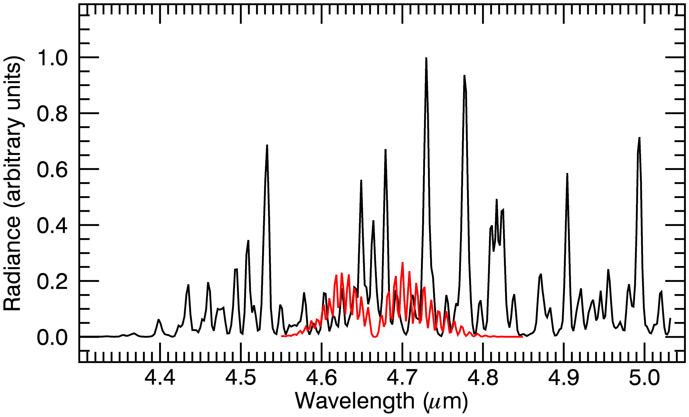
Figure 4: Simulated fluorescence spectra of H₂O (black) and CO (red) for an effective spectral resolution of 800. The CO/H₂O abundance ratio is 1% and the rotational temperature is 100 K.

3.2 The CO₂, ¹³CO₂ complex

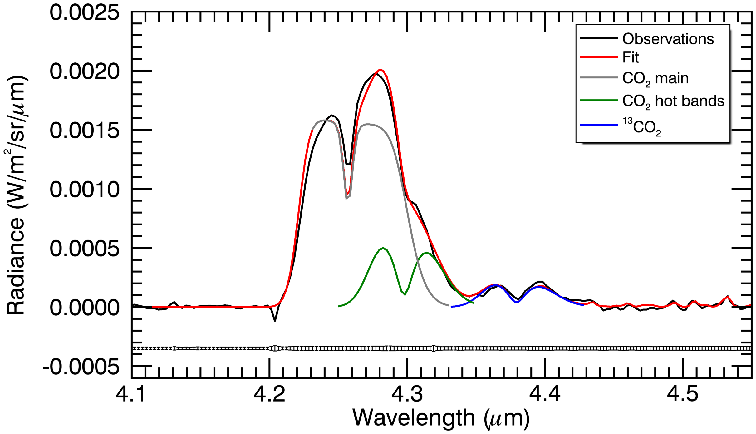
Figure 5: Exemple of model fit to a VIRTIS-H spectrum in the 4.2–4.6 $\mu$m range. The considered spectrum is the mean of four data cubes obtained on 6 and 7 September 2015. Top panel: observed spectrum with standard deviations (black) and model fit (red). Bottom panel: observed spectrum and model fit for each individual band (grey, green and blue lines for CO₂, CO₂ hot bands, and ¹³CO₂, respectively); the continuum radiation due to dust thermal radiation has been removed; standard deviations are given in the bottom of the plot (see Fig. 3). Free model parameters are the baseline polynomial, and multiplying factors to CO₂, ¹³CO₂, and H₂O fluorescence spectra computed for a rotational temperature of 120 K. The ratio between the intensities of the CO₂ hot bands and the ¹³CO₂ band is fixed to the expected value for ¹²CO/¹³CO = 89.

Table 2: Fluorescence g-factors.

Molecule	Band	Wavelength	g-factora	Ref.b
		$\mu$m	s-1
H2O	$\nu_{3}-\nu_{2},\nu_{1}-\nu_{2}$	4.2–5.2	1.40 $\times$ 10-5	(1)
CO2	$\nu_{3}$	4.26	2.69 $\times$ 10-3	(2)
CO2	$\nu_{1}+\nu_{3}-\nu_{1}$	4.30	8.7 $\times$ 10-5c	(3)
13CO2	$\nu_{3}$	4.38	2.42 $\times$ 10-3	(4)
CH4	$\nu_{3}$	3.31	4.0 $\times$ 10-4	(4)
OCS	$\nu_{3}$	4.85	2.80 $\times$ 10-3	(4)

^a The total band g-factors are listed for $r_{h}=1$ AU and scale as $r_{h}^{-2}$. They are computed for $T_{rot}=100$ K (but they only weakly depend upon $T_{rot}$).
^b References: (1) Villanueva et al. (2012); (2) Debout, Bockelée-Morvan, & Zakharov (2016); (3) Crovisier (2009); (4) this work.
^c Sum of the g-factors of the $10^{0}1_{II}-10^{0}0_{II}$ and $10^{0}1_{I}-10^{0}0_{I}$ bands.

The CO₂ $\nu_{3}$ band shows strong fluorescence emission between 4.2 and 4.32 $\mu$m (Fig. 5). A wing in the long wavelength range extending up to about 4.35 $\mu$m is present. It is attributed to fluorescence emission of two hot bands of CO₂, namely the $10^{0}1_{II}-10^{0}0_{II}$ and $10^{0}1_{I}-10^{0}0_{I}$ ($\nu_{1}+\nu_{3}-\nu_{1}$ bands) centred at 2327.4 and 2326.6 cm^-1 (4.30 $\mu$m), respectively. A weak band extending from 4.35 to 4.42 $\mu$m is present, identified as the ¹³CO₂ $\nu_{3}$ band. This is the first detection of ¹³CO₂ and CO₂ hot bands in a comet. In optically thin conditions, these bands are much weaker than the CO₂ main band. A priori, their observation allows a determination of the CO₂ column density independently of transfer modelling. However, some modelling of the spectral shape of the CO₂ main band is required since : i) the hot bands are blended with the $P$ branch of the CO₂ main band in the observations considered here (whereas observations obtained farther from the nucleus in the cold coma show distinctly the $R$ branch of the hot bands); ii) the CO₂ complex is close to the edge of order 0, with little margin for baseline removal.

As in the case of H₂O, we modelled the fluorescence excitation of CO₂ and subsequent cascades in the optically thin approximation following Crovisier (2009), using line strengths and frequencies from the GEISA database (Jacquinet-Husson et al., 2011). The g-factor for the sum of the two hot bands is 3.3% of that of the main band (Table 2). For the $\nu_{3}$ band of ¹³CO₂, synthetic spectra were computed assuming resonant fluorescence and using the HITRAN molecular database (Rothman et al., 2013). The blend of the two hot bands is about three times more intense than the ¹³CO₂ $\nu_{3}$ band for a terrestrial ¹²C/¹³C ratio of 89.

Fluorescence emission from the $\nu_{3}$ band of C¹⁸O¹⁶O is not significant and will not be considered in the spectral analysis. This band is centred at 4.29 $\mu$m, i.e., close to the wavelength of the hot bands. Assuming the terrestrial ¹⁶O/¹⁸O ratio of 500, this band is estimated to be nine times less intense than the blend of the two hot bands.

Sample spectra of the CO₂ $\nu_{3}$ band in optically thick conditions were calculated using a simple approach. For computing the excitation of the excited vibrational state, we used the Escape probability formalism, following Bockelée-Morvan (1987). The intensity of the individual lines [W m^-2 sr^-1] was then computed according to:

$$I_{ul}=\frac{2hcv_{th}}{\lambda^{4}}\frac{p_{u}}{\frac{w_{u}}{w_{l}}p_{l}-p_{u}}(1-e^{-\tau_{ul}}),$$ (1)

with the line opacity $\tau_{ul}$ computed according to:

$$\tau_{ul}=\frac{A_{ul}Nw_{u}}{8\pi\lambda^{3}v_{th}}(\frac{p_{l}}{w_{l}}-\frac{p_{u}}{w_{u}}),$$ (2)

where $\lambda$ is the wavelength, the $u$ and $l$ indices refer to the upper and lower levels of the transition, respectively, with $p_{i}$, $w_{i}$, $A_{ij}$ corresponding to level populations, statistical weights, and Einstein-$A$ coefficient, respectively. This formula assumes thermal line widths described by the thermal velocity $v_{th}$. $N$ is the column density along the LOS. The input parameters of this model are the column density and the rotational temperature. We adjusted these parameters to obtain a CO₂ band shape approximately matching the observed one. Both parameters affect the band shape, that is the width, the relative intensity of the $P$, $R$ branches, and the depth of the valley between the two branches. Because this model is very simplistic (see exact radiative transfer modelling of Debout, Bockelée-Morvan, & Zakharov, 2016), the input parameters that provide good fit to the data will not be discussed.

3.3 CH₄

The $\nu_{3}$ band of CH₄ at 3.31 $\mu$m presents a $P$, $Q$, $R$ structure. The strong $Q$ branch, which is undetectable from ground-based observations due to telluric absorptions, is detected in 75% of the considered VIRTIS-H cubes. The $R$ lines, shortwards of 3.31 $\mu$m, are also well detected when averaging several cubes, with relative intensities consistent with fluorescence modelling (Fig. 6). The discrepancy between the CH₄ fluorescence model and observations longward 3.32 $\mu$m seen in Fig. 6 is caused by the blending of CH₄ $P$ lines with molecular lines from other species. Indeed, ground-based spectral surveys of this spectral region in several comets show number of lines, especially from C₂H₆ and CH₃OH (Dello Russo et al., 2006, 2013). The analysis of the 3.32–3.5 $\mu$m region, characteristic of C-H stretching modes of organic molecules, will be the object of a forthcoming paper.

Synthetic spectra of the $\nu_{3}$ band of CH₄ simulated for various temperatures are shown in Fig. 7. They were computed for resonant fluorescence using the HITRAN database (Rothman et al., 2013). Although some observations point to low nuclear spin temperatures for methane (Kawakita et al., 2005), we assumed the distribution of the $A$, $E$ and $F$ spin species to be equilibrated with the rotational temperature. The low signal-to-noise ratio does not allow us to study the spin distribution from the VIRTIS-H observations. The $Q$ branch, which is an unresolved blend of $\Delta J=0$ lines of the three spin species, has a g-factor which is insensitive to the rotation (and spin) temperature for $T\gtrsim 60$ K. It amounts to 30% of the total band intensity. This branch alone will be used to estimate the CH₄ column density.

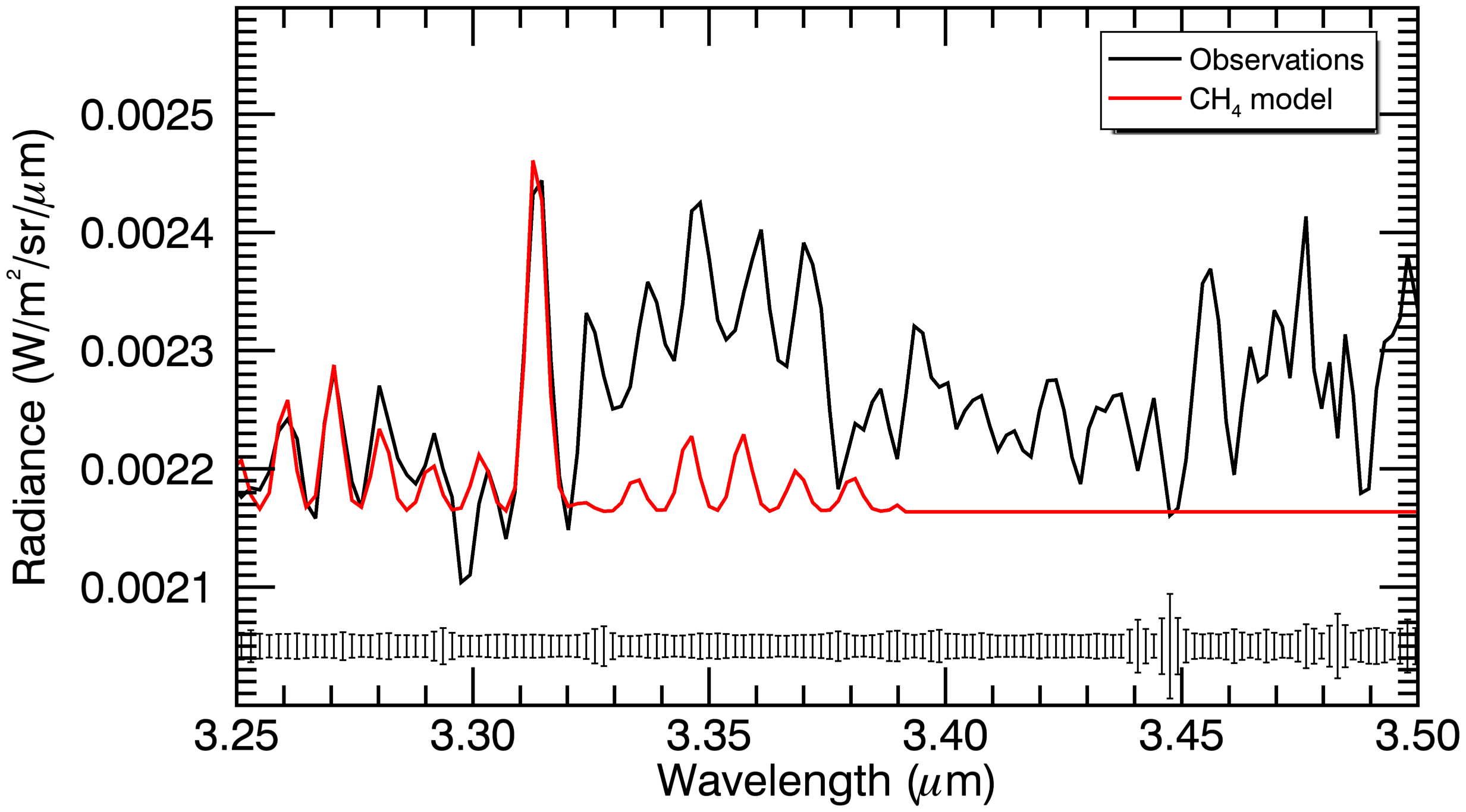
Figure 6: VIRTIS-H spectrum in order 2 covering the CH₄ $\nu_{3}$ band, obtained by averaging 9 data cubes showing well detected CH₄ emission (SNR > 20). The synthetic spectrum of CH₄ computed for a rotational temperature of 100 K is shown in red. The standard deviations are shown in the bottom of the plot (see Fig. 3). Species other than CH₄ (in particular C₂H₆ and CH₃OH) contribute to the signal longward 3.32 $\mu$m.

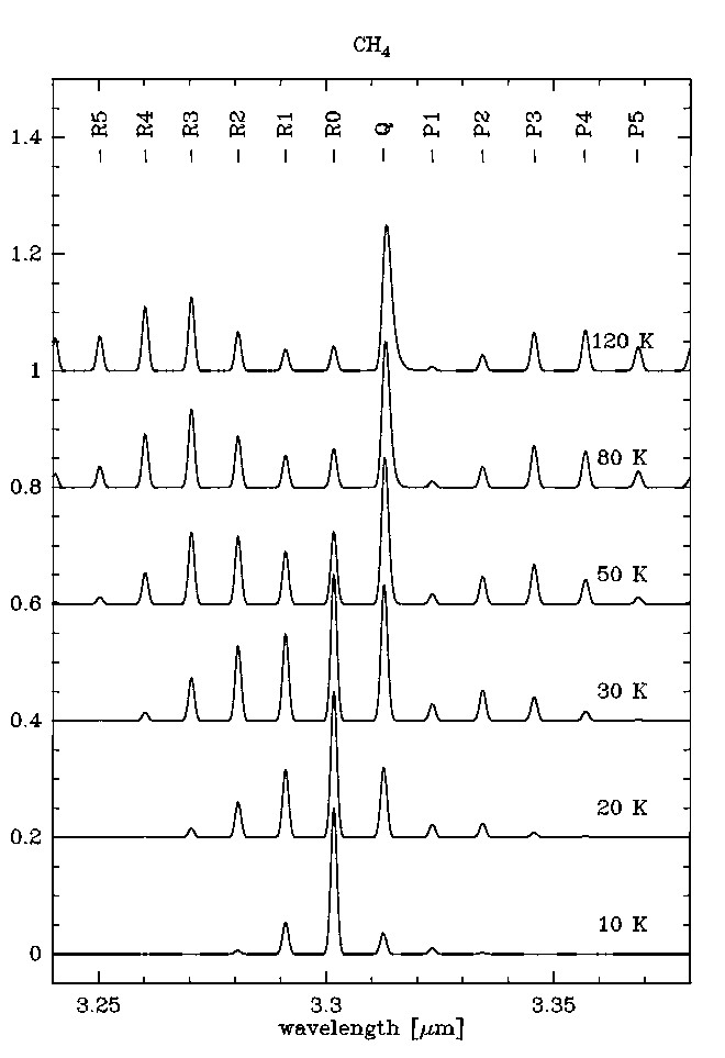
Figure 7: Fluorescence spectra of methane simulated for various rotational temperatures. The $A$, $E$ and $F$ spin species were assumed to be in equilibrium with the rotational temperature. The spectra are normalized to their maximum intensity; note that the spectral resolution is not adjusted to that of the VIRTIS-H instrument.

3.4 OCS and CO

The OCS $\nu_{3}$ band at 4.85 $\mu$m (C–O stretching mode) has a strength comparable to that of the CO₂ $\nu_{3}$ band, allowing its detection even for small column densities in infrared cometary spectra (Dello Russo et al., 1998). In comet 67P, it is detected in most of the data cubes as a faint signal with a peak radiance similar to the strongest water lines nearby (Fig. 3). Our synthetic spectrum follows the model of Crovisier (1987), with a total g-factor of 2.8 $\times$ 10^-3 s^-1 ($r_{h}$ = 1 AU) updated from the HITRAN database (Rothman et al., 2013).

In the same spectral region, with the actual VIRTIS-H spectral resolution, the ro-vibrational lines of the CO ($v=1-0$) band at 4.67 $\mu$m are blended with the lines of water (Fig 4). CO has been detected in comet 67P with the Alice and MIRO instruments (Feldman, personal communication; Biver et al. in preparation) with an abundance relative to water on the order of 1%. With a band g-factor of 2.51 $\times$ 10^-4 s^-1 ($r_{h}$ = 1 AU), based on fluorescence calculations, CO emission is then expected to be faint in VIRTIS spectra. Therefore, the contribution of this band to the spectrum has been neglected in the investigation of the H₂O lines. In Fig 4, the CO spectrum expected for a CO/H₂O abundance ratio of 1% is superimposed on the H₂O spectrum. A tentative estimation of the CO/H₂O abundance based on VIRTIS-H spectra is provided in Sect. 4.

4 Column density and abundance determinations

Table 3: CO₂, ¹³CO₂ $\nu_{3}$ band intensities, and ¹³CO₂ column density.

Start time	$I$(13CO2)	$I$(CO2)	CO2 $\nu_{3}$ atten.a	$N$(13CO2)
(UT)	(10-5 W m-2 sr-1)	(10-5 W m-2 sr-1)		(1018 m-2)
2015-07-08T21:11:00.3	0.90 $\pm$ 0.40b,c	16.20 $\pm$ 0.09b	3$-$7	1.75 $\pm$ 0.77b,c
2015-07-12T11:46:52.6	$-$	$-$	$-$	$-$
2015-07-17T08:15:55.9	0.90 $\pm$ 0.30c	15.40 $\pm$ 0.02	3$-$7	1.70 $\pm$ 0.57c
2015-07-22T15:23:57.9	1.20 $\pm$ 0.20c	30.90 $\pm$ 0.04	3.4	2.20 $\pm$ 0.37c
2015-07-22T21:10:24.7	0.43 $\pm$ 0.11c	16.50 $\pm$ 0.03	2.3	0.80 $\pm$ 0.20c
2015-07-27T23:06:40.5	0.53 $\pm$ 0.09c	14.00 $\pm$ 0.01	2.8	0.97 $\pm$ 0.16c
2015-07-29T21:20:59.8	0.53 $\pm$ 0.03	17.90 $\pm$ 0.04	2.6	0.95 $\pm$ 0.06
2015-07-30T01:47:25.8	0.43 $\pm$ 0.03	17.70 $\pm$ 0.04	2.2	0.78 $\pm$ 0.06
2015-08-01T08:25:16.8	0.87 $\pm$ 0.03	22.70 $\pm$ 0.04	3.4	1.57 $\pm$ 0.05
2015-08-10T23:32:29.0	0.35 $\pm$ 0.03	12.80 $\pm$ 0.04	2.4	0.62 $\pm$ 0.06
2015-08-16T11:56:25.1	1.27 $\pm$ 0.05	23.20 $\pm$ 0.09	4.9	2.25 $\pm$ 0.09
2015-08-19T11:08:06.5	2.34 $\pm$ 0.03	32.50 $\pm$ 0.05	6.4	4.18 $\pm$ 0.06
2015-08-19T15:34:33.4	2.03 $\pm$ 0.04	31.30 $\pm$ 0.07	5.8	3.62 $\pm$ 0.08
2015-08-19T21:20:58.5	2.07 $\pm$ 0.05	24.50 $\pm$ 0.07	7.5	3.69 $\pm$ 0.08
2015-08-20T22:13:06.6	1.51 $\pm$ 0.03	16.80 $\pm$ 0.04	8.0	2.69 $\pm$ 0.05
2015-08-23T17:07:54.5	1.63 $\pm$ 0.03	21.40 $\pm$ 0.05	6.8	2.92 $\pm$ 0.05
2015-08-23T21:29:29.5	1.73 $\pm$ 0.03	20.20 $\pm$ 0.04	7.6	3.10 $\pm$ 0.05
2015-08-26T08:17:52.6	1.59 $\pm$ 0.03	18.70 $\pm$ 0.04	7.6	2.86 $\pm$ 0.06
2015-08-26T10:58:13.4	1.90 $\pm$ 0.08	19.30 $\pm$ 0.11	8.8	3.44 $\pm$ 0.14
2015-09-06T21:25:16.9	0.91 $\pm$ 0.04	12.70 $\pm$ 0.07	6.4	1.71 $\pm$ 0.07
2015-09-07T03:06:16.9	0.96 $\pm$ 0.04	11.60 $\pm$ 0.07	7.4	1.81 $\pm$ 0.07
2015-09-07T07:28:16.8	0.90 $\pm$ 0.05	11.00 $\pm$ 0.07	7.3	1.70 $\pm$ 0.09
2015-09-07T13:09:16.0	0.94 $\pm$ 0.03	12.60 $\pm$ 0.05	6.7	1.78 $\pm$ 0.05
2015-09-09T08:15:16.0	2.03 $\pm$ 0.03	20.90 $\pm$ 0.04	8.7	3.87 $\pm$ 0.06
2015-09-09T15:29:34.0	1.22 $\pm$ 0.02	15.40 $\pm$ 0.03	7.0	2.32 $\pm$ 0.04
2015-09-10T01:37:26.0	0.90 $\pm$ 0.02	11.10 $\pm$ 0.02	7.2	1.71 $\pm$ 0.03
2015-09-13T06:54:44.2	1.44 $\pm$ 0.02	16.90 $\pm$ 0.02	7.6	2.81 $\pm$ 0.04
2015-09-13T11:46:19.3	1.77 $\pm$ 0.08	18.50 $\pm$ 0.13	8.5	3.45 $\pm$ 0.16
2015-09-24T11:55:21.0	0.64 $\pm$ 0.01	9.06 $\pm$ 0.02	6.3	1.34 $\pm$ 0.03
2015-09-27T16:57:54.5	0.32 $\pm$ 0.01	4.89 $\pm$ 0.01	5.8	0.68 $\pm$ 0.03

^a Attenuation factor of the CO₂ $\nu_{3}$ band, corresponding to the ratio between the $\nu_{3}$ band intensity expected in optically thin conditions and the observed $\nu_{3}$ band intensity (see text).

^b Results obtained by averaging the data of 8 and 12 July.

^c Values and uncertainties cover results obtained using either multi-component fit or the ¹³CO₂ band area measured on the spectrum.

Table 4: H₂O, CH₄ and OCS band intensities and column densities.

Start time	H2O		CH4		OCS
	————————————-		————————————-		————————————-
	$I$	$N^{b}$	$I^{a}$	$N^{c}$	$I^{a}$	$N^{c}$
(UT)	(10-5 W m-2 sr-1)	(1020 m-2)	(10-6 W m-2 sr-1)	(1018 m-2)	(10-6 W m-2 sr-1)	(1018 m-2)
2015-07-08T21:11:00.3	1.82 $\pm$ 0.56	9.25 $\pm$ 2.88	$-$0.69 $\pm$ 0.48	$-$0.62 $\pm$ 0.44	6.87 $\pm$ 3.34	1.31 $\pm$ 0.63
2015-07-12T11:46:52.6	1.90 $\pm$ 0.14	10.10 $\pm$ 0.77	$-$3.42 $\pm$ 0.17	$-$3.04 $\pm$ 0.15	$-$2.63 $\pm$ 0.86	$-$0.49 $\pm$ 0.16
2015-07-17T08:15:55.9	1.22 $\pm$ 0.07	6.33 $\pm$ 0.36	$-$0.56 $\pm$ 0.14	$-$0.49 $\pm$ 0.12	8.82 $\pm$ 0.40	1.60 $\pm$ 0.07
2015-07-22T15:23:57.9	1.86 $\pm$ 0.08	10.00 $\pm$ 0.41	3.50 $\pm$ 0.13	2.97 $\pm$ 0.11	9.50 $\pm$ 0.48	1.68 $\pm$ 0.09
2015-07-22T21:10:24.7	1.90 $\pm$ 0.05	9.79 $\pm$ 0.28	$-$1.84 $\pm$ 0.12	$-$1.56 $\pm$ 0.10	3.49 $\pm$ 0.37	0.62 $\pm$ 0.06
2015-07-27T23:06:40.5	1.49 $\pm$ 0.04	6.48 $\pm$ 0.17	1.78 $\pm$ 0.10	1.48 $\pm$ 0.08	2.03 $\pm$ 0.28	0.35 $\pm$ 0.05
2015-07-29T21:20:59.8	1.49 $\pm$ 0.10	6.62 $\pm$ 0.44	$-$1.10 $\pm$ 0.17	$-$0.91 $\pm$ 0.14	5.00 $\pm$ 0.61	0.87 $\pm$ 0.11
2015-07-30T01:47:25.8	1.63 $\pm$ 0.11	7.27 $\pm$ 0.48	1.85 $\pm$ 0.17	1.53 $\pm$ 0.14	4.93 $\pm$ 0.64	0.85 $\pm$ 0.11
2015-08-01T08:25:16.8	1.63 $\pm$ 0.09	7.10 $\pm$ 0.39	2.99 $\pm$ 0.35	2.46 $\pm$ 0.29	5.93 $\pm$ 0.63	1.02 $\pm$ 0.11
2015-08-10T23:32:29.0	1.17 $\pm$ 0.11	4.19 $\pm$ 0.40	1.72 $\pm$ 0.29	1.40 $\pm$ 0.24	$-$2.99 $\pm$ 0.67	$-$0.51 $\pm$ 0.11
2015-08-16T11:56:25.1	2.01 $\pm$ 0.14	9.21 $\pm$ 0.63	2.58 $\pm$ 0.25	2.09 $\pm$ 0.20	6.43 $\pm$ 0.86	1.09 $\pm$ 0.15
2015-08-19T11:08:06.5	2.02 $\pm$ 0.10	10.20 $\pm$ 0.50	7.77 $\pm$ 0.16	6.33 $\pm$ 0.13	16.50 $\pm$ 0.65	2.82 $\pm$ 0.11
2015-08-19T15:34:33.4	2.42 $\pm$ 0.13	11.60 $\pm$ 0.64	5.40 $\pm$ 0.18	4.40 $\pm$ 0.15	16.90 $\pm$ 0.79	2.89 $\pm$ 0.13
2015-08-19T21:20:58.5	1.97 $\pm$ 0.13	8.90 $\pm$ 0.61	4.93 $\pm$ 0.22	4.02 $\pm$ 0.18	13.80 $\pm$ 0.79	2.36 $\pm$ 0.14
2015-08-20T22:13:06.6	2.03 $\pm$ 0.09	8.32 $\pm$ 0.38	6.83 $\pm$ 0.17	5.57 $\pm$ 0.14	9.54 $\pm$ 0.53	1.63 $\pm$ 0.09
2015-08-23T17:07:54.5	1.89 $\pm$ 0.08	8.27 $\pm$ 0.33	4.52 $\pm$ 0.18	3.71 $\pm$ 0.15	9.03 $\pm$ 0.48	1.55 $\pm$ 0.08
2015-08-23T21:29:29.5	1.65 $\pm$ 0.08	7.44 $\pm$ 0.36	5.53 $\pm$ 0.24	4.54 $\pm$ 0.20	8.07 $\pm$ 0.51	1.39 $\pm$ 0.09
2015-08-26T08:17:52.6	1.63 $\pm$ 0.08	6.87 $\pm$ 0.36	4.92 $\pm$ 0.41	4.06 $\pm$ 0.34	6.01 $\pm$ 0.70	1.04 $\pm$ 0.12
2015-08-26T10:58:13.4	2.14 $\pm$ 0.23	9.30 $\pm$ 0.99	7.38 $\pm$ 0.36	6.09 $\pm$ 0.30	7.73 $\pm$ 1.30	1.34 $\pm$ 0.23
2015-09-06T21:25:16.9	1.28 $\pm$ 0.12	5.25 $\pm$ 0.49	2.04 $\pm$ 0.22	1.76 $\pm$ 0.19	$-$2.11 $\pm$ 0.69	$-$0.38 $\pm$ 0.12
2015-09-07T03:06:16.9	1.37 $\pm$ 0.11	5.64 $\pm$ 0.43	$-$0.99 $\pm$ 0.20	$-$0.85 $\pm$ 0.17	3.91 $\pm$ 0.64	0.71 $\pm$ 0.12
2015-09-07T07:28:16.8	0.89 $\pm$ 0.15	3.64 $\pm$ 0.60	2.23 $\pm$ 0.25	1.93 $\pm$ 0.22	$-$1.98 $\pm$ 0.83	$-$0.36 $\pm$ 0.15
2015-09-07T13:09:16.0	1.30 $\pm$ 0.09	5.35 $\pm$ 0.35	3.71 $\pm$ 0.19	3.20 $\pm$ 0.16	$-$3.32 $\pm$ 0.54	$-$0.60 $\pm$ 0.10
2015-09-09T08:15:16.0	1.60 $\pm$ 0.09	8.22 $\pm$ 0.49	3.33 $\pm$ 0.24	2.90 $\pm$ 0.21	8.76 $\pm$ 0.59	1.59 $\pm$ 0.11
2015-09-09T15:29:34.0	1.56 $\pm$ 0.06	7.42 $\pm$ 0.30	4.12 $\pm$ 0.12	3.59 $\pm$ 0.11	6.13 $\pm$ 0.41	1.12 $\pm$ 0.08
2015-09-10T01:37:26.0	1.23 $\pm$ 0.04	4.93 $\pm$ 0.18	$-$3.69 $\pm$ 0.23	$-$3.23 $\pm$ 0.20	3.56 $\pm$ 0.34	0.65 $\pm$ 0.06
2015-09-13T06:54:44.2	1.47 $\pm$ 0.06	7.13 $\pm$ 0.29	3.71 $\pm$ 0.13	3.30 $\pm$ 0.12	7.40 $\pm$ 0.39	1.38 $\pm$ 0.07
2015-09-13T11:46:19.3	2.11 $\pm$ 0.21	10.00 $\pm$ 1.00	$-$2.93 $\pm$ 0.59	$-$2.61 $\pm$ 0.53	7.41 $\pm$ 1.13	1.38 $\pm$ 0.21
2015-09-24T11:55:21.0	0.81 $\pm$ 0.04	3.68 $\pm$ 0.19	4.07 $\pm$ 0.13	3.88 $\pm$ 0.12	$-$-0.06$\pm$ 0.32	$-$-0.01$\pm$ 0.06
2015-09-27T16:57:54.5	0.56 $\pm$ 0.04	2.41 $\pm$ 0.18	2.15 $\pm$ 0.13	2.10 $\pm$ 0.12	$-$0.87 $\pm$ 0.30	$-$0.18 $\pm$ 0.06

^a Only values obtained when detection are given.

^b Derived assuming a gas kinetic temperature varying with distance to comet centre ($\rho$) following $T_{kin}$ = (4/$\rho$[km]) $\times$ 100 K (with $T_{rot}$ = $T_{kin}$) and a g-factor of 1.19 $\times$ 10^-5 at 1 AU from the Sun pertaining to the 4.45–5.03 $\mu$m range.

^c Derived assuming $T_{rot}$ = 100 K in the fluorescence model.

4.1 Fitting procedure

Observed spectra were analysed using the Levenberg-Marquardt $\chi^{2}$ minimization algorithm, describing the spectra as a linear combination of a background continuum (polynomial) and fluorescence molecular emissions, modelled as presented in Sect. 3 and convolved to the spectral resolution of the analysed data (Sect. 2.1).

In the fitting procedure, the rotational temperature of the molecules was taken as a fixed parameter. In dense parts of the coma, the rotational states in the ground-vibrational state of the molecules are expected to be thermalized to the gas kinetic temperature, so that $T_{rot}$ = $T_{kin}$ locally. However, since the coma is not isothermal, VIRTIS spectra mix contributions of molecules at various $T_{rot}$, implying a ro-vibrational structure which depends in a complex way on the temperature and gas distributions, but which should reflect conditions in the denser parts of the coma probed by the VIRTIS LOS. We adopted a simplistic approach, and fixed $T_{rot}$ according to available information for comet 67P. Indeed, molecular data obtained by the MIRO instrument onboard Rosetta show that the gas kinetic temperature follows in first order $T_{kin}$[K] = (4 [km]/$\rho$[km]) $\times$ 100 [K] for $\rho$ in the range 3–25 km, where $\rho$ is the distance to comet centre (Biver, personal communication). The corresponding temperatures we used for the VIRTIS-H data showing detected CH₄ and OCS emissions are thus 80–130 K. We found that adopting specific temperatures for each data cube does not change significantly the results for CH₄ and OCS since the intensities of the CH₄ $Q$ branch and of the OCS band are not sensitive to the temperature (above 60 K for CH₄). We assumed $T_{rot}$ = 100 K for the fluorescence emissions of CH₄ and OCS. For H₂O, CO₂ hot-bands, and ¹³CO₂, the fit was performed for appropriate values of $T_{kin}$.

We used optically thick CO₂ spectra (Sect. 3.2) that provide reasonable fits to the CO₂ $\nu_{3}$ band and to the overall CO₂ complex, with a multiplying coefficient to the synthetic spectrum as a free parameter. The ¹²CO₂/¹³CO₂ relative abundance was assumed to be terrestrial, that is the intensity of the CO₂ hot-bands relative to the ¹³CO₂ band was fixed to be equal to 89 times the ratio of the g-factors.

The CO₂ complex was analysed by fitting the whole 4.05–4.8 $\mu$m region, hence excluding the OCS band but including H₂O emission lines. Conversely, the H₂O and OCS emissions were studied considering the 4.45–5.01 $\mu$m region, i.e., excluding the CO₂ complex. CO fluorescence emission was assumed to be negligible (Sect 3.4). For the CH₄ band, the fit was performed in the 3.25–3.322 $\mu$m region, ignoring the region where $P$ lines are blended with other molecular lines. The fitting algorithm was successful in fitting the CH₄ $Q$ branch. The degree of the polynomial used to fit the baseline was fixed to 2 for the CH₄ study, to 4 for H₂O and OCS, and to 5 for the CO₂ complex. Smaller polynomial degrees provided often unsatisfactory results for the continuum background observed in order 0, which is due to dust thermal emission superimposed with some instrumental stray light at the shortest wavelengths (see Sect. 2.1).

An example of the result of the fitting procedure to the CO₂ complex is presented in Fig. 5, where the individual components are plotted. Other fits for different data sets are illustrated in Fig. 8. For most individual data cubes, the ¹³CO₂ band is detected distinctly and the band intensity retrieved from the fit is well estimated. However, for the six first data cubes (8–27 July), the method led to an underestimation of the ¹³CO₂ signal (as observed visually): the model fit fell below the observed ¹³CO₂ emission. For these 6 observations, we also computed the intensity in the 4.34–4.42 $\mu$m range lying above the background, and the intensities computed by the two methods were taken as providing the range of possible values for the ¹³CO₂ band intensities. We note that often the model fails to fully reproduce the intensity of the $P$ branch of ¹³CO₂ (some residual is present at 4.4 $\mu$m, Fig. 8). The origin of this residual is unclear.

Examples of model fits to the H₂O and OCS emissions are shown in Fig. 3. For this spectral region, we identified a shift by about 1 spectral channel (2.2 nm) between the expected and observed position of the water lines. The shift is observed specifically for the lines in the 4.6–4.8 $\mu$m range, whereas the water lines shortward 4.6 $\mu$m suggest an error in the present spectral calibration by 1/2 channel. Therefore, the observed spectra were shifted by one channel when fitting the H₂O and OCS emissions (also for Fig. 3). However, we didn’t apply any correction for fitting the CO₂ complex. Earth and Mars spectra taken with VIRTIS-H suggests an error of 1/2 pixel in the spectral registration. We expect further progress in the VIRTIS-H spectral calibration in the future. A close examination of the 67P spectra plotted in Fig. 3 shows some mismatch for the intensity of the H₂O lines, that may deserves further studies. In particular, the line at 4.81 $\mu$m is observed in all 67P spectra, and is most likely of cometary origin. Though water emission is expected at this wavelength, the intensity of this line is not consistent with water synthetic spectra (Figs 3– 4).

A critical point in the analysis is the estimation of uncertainties. For the staring observations, the root-mean-square (rms) deviations can be estimated for each spectral channel by studying the variation with time of their intensity (computation of variance, then rms). However, for data cubes showing comet signal, the rms computed in this way are larger than statistical instrumental noise, since part of the variation is intrinsic to the comet and/or pointing mode. All uncertainties provided in the tables and figures include the dispersion due to the varying intrinsic comet signal (including the continuum). In Fig. 3A, we have superimposed the rms measured on a data cube presenting little comet signal, which is effectively much lower than the one computed with the adopted method. However, based on the fluctuations seen on the spectra, we believe that using instead these rms would underestimate uncertainties.

A number of spectral channels are much noiser than their neighbors (so-called "hot pixels"). "Hot pixels" can be spotted in Figs 3, 5, and 6 from their higher errors. There are no hot pixels for the channels covering the CH₄ $Q$-branch (Fig. 6). The fitting of H₂O lines was performed by ignoring the very few "hot pixels" near the water lines. The OCS band is also affected by hot pixels (see Fig. 3). These were not masked in the fitting analysis. The discrepancy observed at 4.87 $\mu$m between model fit and observed OCS band (see Fig. 3) is possibly of instrumental origin.

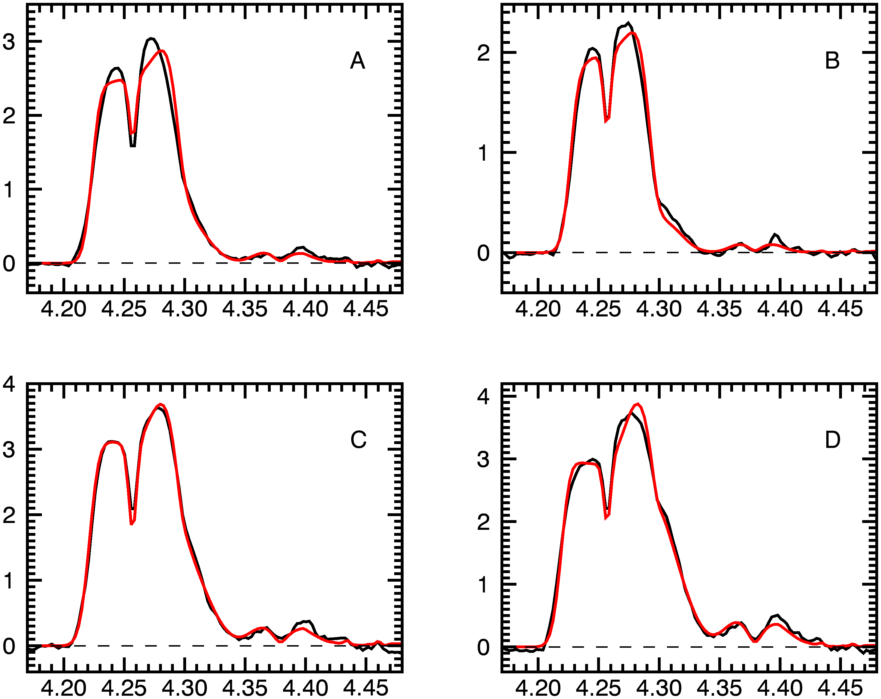
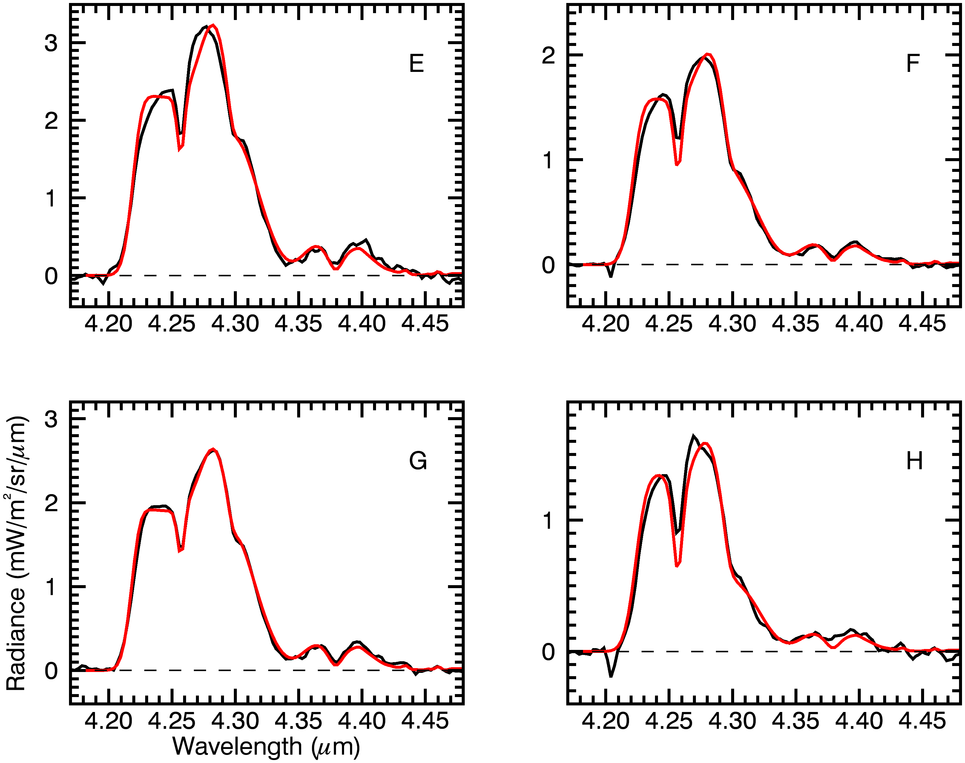
Figure 8: VIRTIS-H spectra in the 4.2–4.5 $\mu$m region (black), and model fits (red) to the CO₂ and ¹³CO₂ bands. The continuum background is removed. A : 29–30 Jul., 1 Aug.; B: 10 Aug.; C: 16 Aug.; D: 19–23 Aug; E: 26 Aug.; F: 6–7 Sept; G: 9–13 Sept.; H: 24 Sept.

4.2 Results

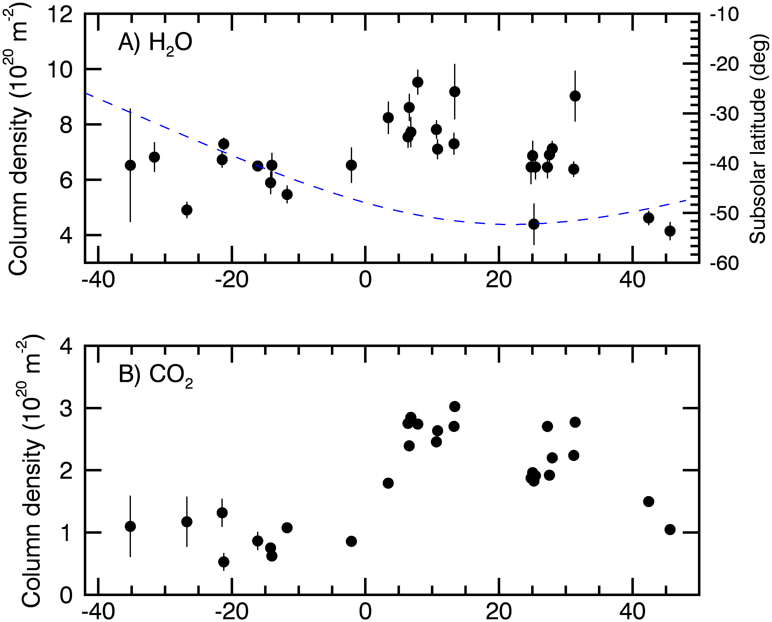
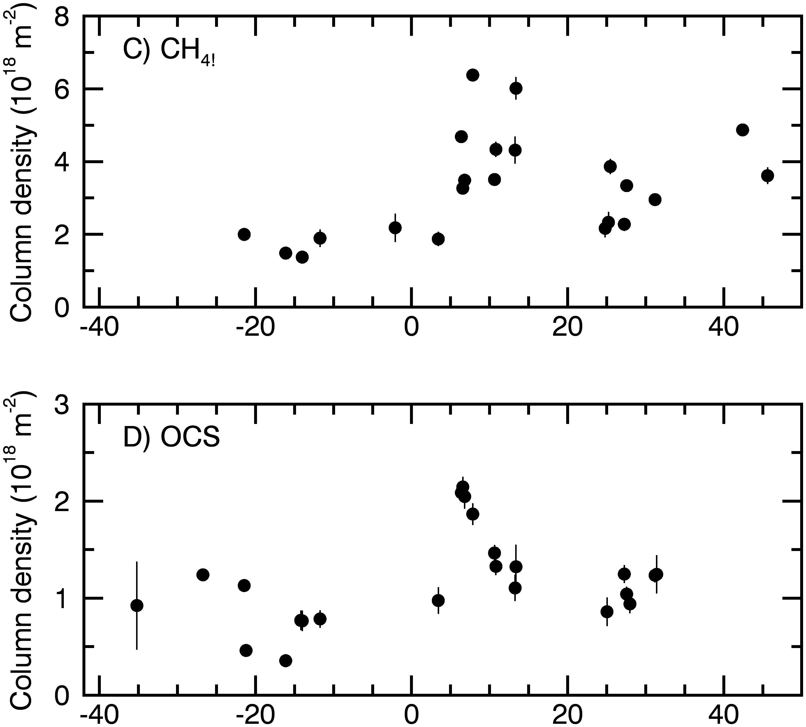
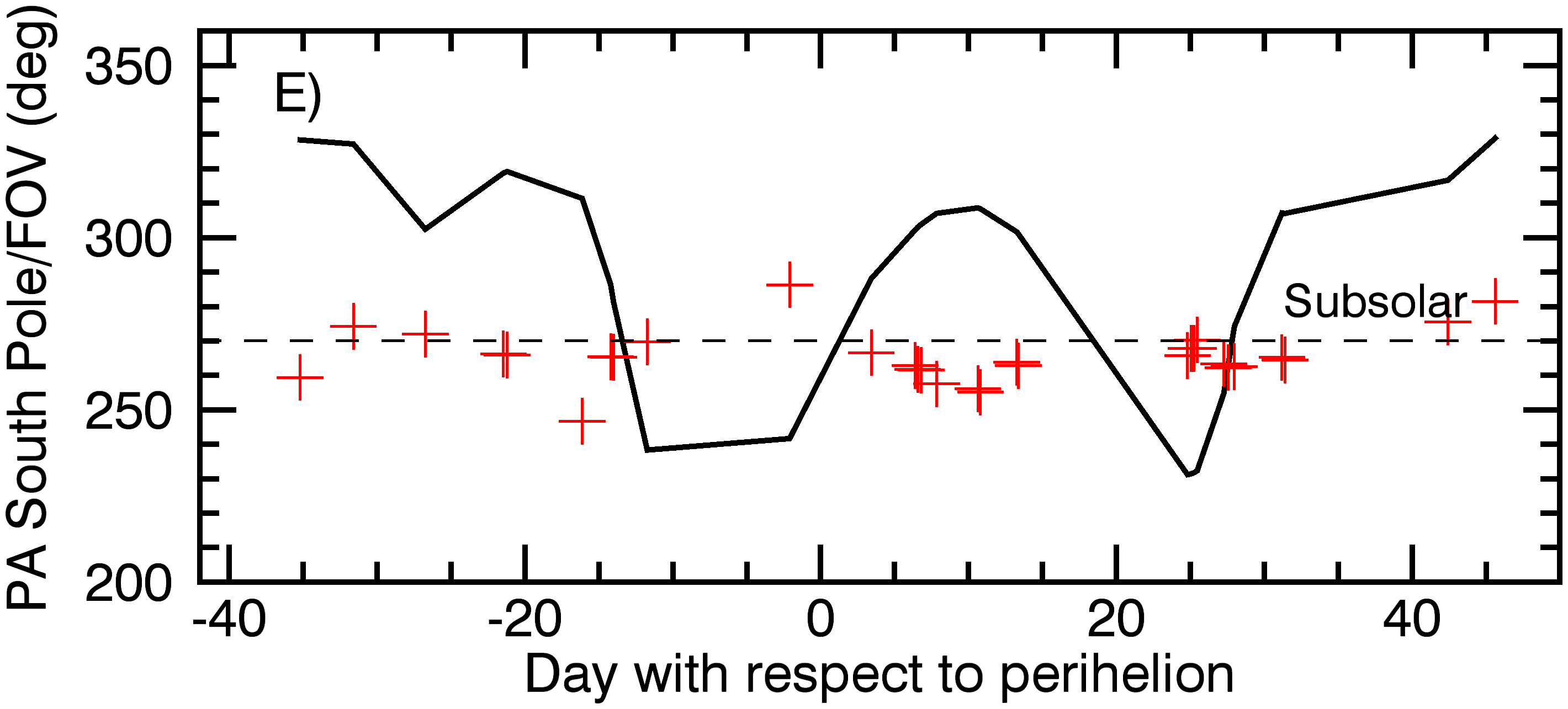
Figure 9: Column densities of H₂O, CO₂, CH₄ and OCS as a function of date with respect to perihelion (A–D), and position angles of the South pole direction and FOV (E). A–D) Measured column densities (dots with error bar) are rescaled to a distance of $\rho$ = 4 km assuming a 1/$\rho$ variation; the latitude of the subsolar point is plotted as a dashed line in plot A. E) The PA of the South direction is shown as a black line; the PA of the FOV are plotted with crosses; the projected comet-Sun direction at $PA$ = 270^∘ is indicated as a dashed line.

Band intensities ($I$) and column densities ($N$) obtained from fitting are listed in Table 3 for CO₂, and in Table 4 for H₂O, OCS, and CH₄. Regarding CO₂, we also provide the attenuation factor $f_{atten}$ of the main band which is determined from the CO₂ and ¹³CO₂ $\nu_{3}$ band intensities according to $f_{atten}$ = 89 $\times$ $I$(¹³CO₂)/$I$(CO₂). The attenuation factor corresponds to the ratio between the $\nu_{3}$ band intensity expected in optically thin conditions and the observed $\nu_{3}$ band intensity. This factor reaches values of 2 to 9. The varying correlation between CO₂ band intensity and attenuation factor is expected from radiative transfer calculations, because of azimuthal variations of local excitation related to the uni-directionality of the excitation source and to the 3D structure of the gas velocity field (Gersch & A’Hearn, 2014; Debout, Bockelée-Morvan, & Zakharov, 2016).

Column densities provide partial information of the overall activity of the comet because: i) the FOV is sampling a small fraction of the coma at a location in the gaseous fan which is each time different (Sect. 2.3); ii) 67P’s nucleus shape and outgassing behavior is complex, and we indeed observe rotation-induced variations of column densities (see results for 19 August). The evolution of the water column density in VIRTIS-H field of view is plotted in Fig. 9 for $\rho$ = 4 km. We corrected for the different distances from comet centre of the FOV assuming a 1/$\rho$ variation (but we did not correct for possible gas velocity variations). The low H₂O column density observed for September 24, 27 (the two last data points) is likely related to the small phase angle, as already discussed in Sect. 2.2. The measured column densities are consistent with those measured with the MIRO instrument (Biver et al. in preparation).

In order to constrain somewhat the CO abundance relative to water from VIRTIS-H spectra, spectral fitting of the 4.45–5.01 $\mu$m region with a model including CO fluorescence emission, in addition to H₂O and OCS emissions, has been performed. Retrieved values are between 1 and 2%, and consistent with Alice and MIRO results (Feldman, personal communication; Biver et al. in preparation). However, we estimate that further analyses on spectra obtained with an improved calibration are required to claim a CO detection in VIRTIS-H spectra.

An increase of water production a few days after perihelion is suggested from the column density, which is not related to the observing geometry (i.e., to a FOV positionned in a denser part of the gas fan at that time, Fig. 9A). This increase is consistent with the analysis of the VIRTIS-H H₂O raster maps obtained regularly from July to November, which show that the water fan had its maximum brightness 6–7 days after perihelion (Bockelée-Morvan et al., 2016). Therefore, the measured relative abundances should be representative of the composition of the material released from the main outgassing areas in the July–September time frame. Concomitant with the 50% increase of the water column density, a strong increase of the column densities (by factors 2–3) of CO₂, CH₄ and OCS is also observed (Fig. 9B–D).

Figure 10 presents column density ratios, with water taken as the reference (hereafter referred to as relative abundances). A large increase of the CO₂ to H₂O abundance ratio is measured, starting after perihelion, reaching values in the range 30–40% from 19 August (i.e., 6 days after perihelion) and thereafter. This increase in the CO₂/H₂O abundance coincides with the increase in water production. The same trend is observed for CH₄, whereas the evolution of the OCS abundance is somewhat chaotic, reaching however its peak value on 19 August. Averaging data, there is typically a factor of 1.5 increase between OCS abundances measured pre-perihelion and post-perihelion (Table 5). Noteworthy, the investigated post-perihelion period corresponds to the illumination of the most southern latitudes (latitude of the subsolar point $\sim$ –50^∘, Fig. 9).

For the discussion in Sect. 5, we will assume that column density ratios are representative of production rate ratios. This is a good approximation if the spatial distributions of the molecules are similar. However, as judged from the brightness distribution of the CO₂ and H₂O optically thick bands (Sect. 2.3), the angular width of the CO₂ fan is smaller than that of the H₂O fan. Therefore, the CO₂/H₂O production rate ratio from the most active reagions is possibly underestimated.

Table 5: Abundances relative to water.

Molecule	Pre-perihelion	Post-perihelion
	8 Jul.–10 Aug. 2015	16 Aug.–27 Sep. 2015
	(%)	(%)
CO2	14	32
CH4	0.23	0.47
OCS	0.12	0.18

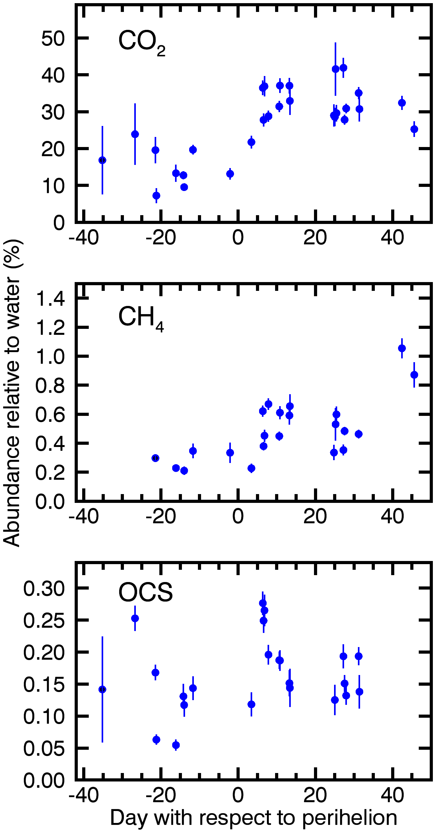
Figure 10: Column density ratios relative to water as a function of day with respect to perihelion.

5 Discussion

The distributions of H₂O and CO₂ in the inner coma of 67P have been measured by several Rosetta instruments since 2014, allowing the investigation of their local, diurnal and seasonal variations. During pre-equinox, the water outgassing was found to follow solar illumination, with, however, an excess of production from the Hapi region in the neck/north pole area, which photometric properties suggest enrichment in surface ice (Fornasier et al., 2015a; De Sanctis et al., 2015; Filacchione et al., 2016b). The CO₂/H₂O column density ratio above the illuminated Hapi region was measured to be small. Ratios in the range 1–3% were determined from VIRTIS data for the November 2014 to April 2015 period (Bockelée-Morvan et al., 2015; Migliorini et al., 2016). Similar values were measured above other regions of the northern hemisphere (Bockelée-Morvan et al., 2015; Migliorini et al., 2016). These values are consistent with measurements at 3 AU from the Sun made by ROSINA (Le Roy et al., 2015). On the other hand, a large CO₂ outgassing from the non-illuminated southern hemisphere was observed, indicating a strong dichotomy between the two hemispheres with subsurface layers much richer in CO₂ in the southern regions (Luspay-Kuti et al., 2015; Migliorini et al., 2016; Fink et al., 2016). From annulus measurements surrounding the comet, Fink et al. (2016) inferred a CO₂/H₂O total production rate ratio of 3–5 % from data obtained in February and April 2015. This ratio is not diagnostic of the relative amount of gases released from a specific region, because of the disparate origin of the two molecukes. ROSINA measurements showed that the distribution of polar molecules is correlated with the H₂O distribution (HCN, CH₃OH), whereas that of apolar and more volatile species (CO, C₂H₆) is correlated with the CO₂ distribution (Luspay-Kuti et al., 2015). However, apolar CH₄ displayed an intriguing distinct behavior from both CO₂ and water (Luspay-Kuti et al., 2015). The CH₄/CO₂ ratio from the northern and southern hemispheres at 3 AU from the Sun was estimated to be 5 and 0.7%, respectively from measurements with ROSINA (Le Roy et al., 2015). As for the CH₄/H₂O ratio it was estimated to 0.1% above the northern summer hemisphere (Le Roy et al., 2015). At 3 AU from the Sun, 67P was releasing small amounts of OCS: OCS/H₂O of 0.02% above the northern hemisphere and OCS/CO₂ of 0.1 % above the southern hemisphere.

In this paper, we investigated outgassing from the southern regions when illuminated by the Sun. These regions were clearly much more productive than during the southern winter time. Using column densities at 4 km from the surface as a proxy of activity, $N$(CO₂) increased typically from $\sim$ 10¹⁹ m^-2 at $r_{h}$ = 1.9 AU (Migliorini et al., 2016) to a few 10²⁰ m^-2 at perihelion time (Table 3). The CH₄/CO₂ ratio remained within a factor of 2 the value measured at 3 AU, whereas the OCS/CO₂ ratio increased by a factor of 6–9. Comparing now the relative amounts (with respect to water) of gases released from the two hemispheres when illuminated (keeping in mind the different heliocentric distances), the southern hemisphere is up to a factor of 10 more productive in CO₂ and OCS relative to water, and by a factor of 2–5 more productive in CH₄. Table  6 summarizes relative abundances measured above the two hemispheres at different seasons.

This seasonal variation in relative molecular abundances is related to the strong differences in illumination conditions experienced by the two hemispheres. The northern hemisphere experiences a long summer but at large heliocentric distances, implying low sublimation rates and very low surface ablation. Though 67P surface and subsurface layers present a low thermal inertia, a stratification in the ice composition is expected, with the more volatile species residing in deeper layers. The residence level of the volatile ices may be at a few tens centimeters from the surface, down to several meters, depending on the volatility of the ice (CO₂, OCS, CH₄ in increasing order of volatility), the dust mantle thickness, thermal inertia, porosity, and illumination history (Marboeuf & Schmitt, 2014). The detection of low levels of CO₂ production from the northern hemisphere indicates that probably most of the CO₂ ice was below the level of the thermal wave, with only a small portion of CO₂ ice reached by the heat. Based on modelling, the CO₂/H₂O ratio measured in the northern hemisphere during summer (1–3 %) should be lower than the nucleus undifferentiated value (Marboeuf & Schmitt, 2014). In other words, values measured in the northern hemisphere are not original, but the result of the devolatilization of the uppermost layers.

The increased gaseous activity of comet 67P as it approached the Sun led to the removal of devolatilized dust, thereby exposing less altered material to the Sun. Evidence for rejuvenation of the surface of 67P is given by a significant increase of the single scattering albedo and more bluish colors as 67P approached the Sun (Filacchione et al., 2016b; Ciarnello et al., 2016). The absence of wide spread smooth or dust covered terrains in the southern hemisphere, together with the presence of large bright ice-rich areas (El-Maarry et al., 2016; Fornasier et al., 2015b) are lines of evidence that this hemisphere was subjected to strong ablation during the perihelion period. Models of the thermal evolution of 67P predict that the depth of ablation should have reached the underlayers where volatile ices are present (De Sanctis et al., 2010b; Marboeuf & Schmitt, 2014). The observed enhancement of the CO₂/H₂O, CH₄/H₂O, and OCS/H₂O abundance ratios could be the result of this ablation. Once the removal of devolatilized layers has proceeded, sustained dust removal due to the sublimation of water ice maintained volatile-rich layers near the surface, as suggested by the abundance ratios which remained high long after perihelion (Fig.10). This requires the erosion velocity to be comparable or larger than the propagation velocity of the diurnal heat, a property expected near perihelion for low thermal inertia material (Gortsas et al., 2011). Should ablation have reached non-differentiated layers, abundances relative to water measured in the coma would then be representative of the nucleus initial ice composition. Simulations performed for comet 67P by Marboeuf & Schmitt (2014) (though not considering the large obliquity of the spin axis) indeed predict a CO₂/H₂O production rate ratio near perihelion similar to the primitive composition of the nucleus for active regions not covered by a thick dust mantle. This model includes diurnal and seasonal recondensation of gases in the colder layers. A result of these simulations is that this process is ineffective in altering the CO₂/H₂O production rate ratio from the southern hemisphere due to the strong erosion. Further modelling of 67P activity may provide alternative interpretations.

OCS is only slightly more volatile than CO₂ with a sublimation temperature of 57 K to be compared to 72 K for the latter species (Yamamoto, 1985). Therefore we should expect similar production curves, if these species are present in icy form. The mean OCS/CO₂ ratios measured pre and post-perihelion in the 7 July to 27 September 2015 period are effectively similar (0.6–0.9 %, Table 6) and comparable to the value measured above the northern hemisphere at 3 AU from the Sun by ROSINA (Le Roy et al., 2015). However, the OCS/CO₂ ratio measured above the southern hemisphere at 3 AU from the Sun is 7 times lower (Le Roy et al., 2015). Possibly, this means that the thermal wave did not reach OCS-rich layers. Also, looking to the individual VIRTIS data obtained in the perihelion period, fluctuations in the OCS/CO₂ ratio are observed, possibly related to compositional or structural heterogeneities. A better understanding of the differences in OCS and CO₂ outgassing would need a larger data set (as that obtained by ROSINA).

As in the case of CO₂, the observed large increase in CH₄ column density and CH₄/H₂O ratio at perihelion is consistent with a CH₄ outgassing front near the surface. The evolution of the sublimation interface of CH₄ pure ice, which is more volatile than CO₂ ice, has been examined by Marboeuf & Schmitt (2014). In this model, the ablation does not reach the CH₄ ice front, and no significant enhancement in CH₄ production is expected at perihelion. However, a large increase in CH₄ production would occur for CH₄ trapped in amorphous ice as the ablation reaches the crystallisation front, or for CH₄ encaged in a clathrate hydrate structure. In the model of Marboeuf & Schmitt (2014), an obliquity of 0^∘ is assumed, and results are provided for equatorial latitudes. Results obtained considering the 52^∘ obliquity of 67P spin axis are given by De Sanctis et al. (2010b) for CO and CO₂ present in icy form. Contrary to Marboeuf & Schmitt (2014), this model predicts a strong outgassing of both CO₂ and CO in the south hemisphere at perihelion. This is because the important erosion that takes place in these regions during their short summer maintains the sublimation interface of volatile species as CO and CH₄ close to the surface.

The CH₄/H₂O ratio exhibits much less contrasting regional and seasonal variations than observed for CO₂ (Table 6). Howewer, the same trend is observed. The maximum value is for South/winter, the minimum value is for North/summer, whereas the intermediate value is for South/summer. This might suggest that they are in a similar form and located in layers close to each other. Should CH₄ and CO₂ be both present in icy form, then less contrasted variations are expected for CH₄ because of its smaller sublimation temperature. Alternatively, CH₄ could be trapped in amorphous water ice inside 67P nucleus and released during ice crystallization, which occurs at a temperature a little below that of water ice sublimation. This could explain the small difference in CH₄/H₂O ratios measured above the two hemispheres during summer time. However, this scenario cannot explain the significant CH₄ outgassing from the non-illuminated hemisphere at 3 AU from the Sun (Luspay-Kuti et al., 2015). Luspay-Kuti et al. (2016) propose the presence of CH₄ clathrate hydrates to explain the behavior observed by ROSINA.

The column densities of H₂O, CO₂, CH₄ and OCS show an abrupt increase at about 6 days after perihelion (Fig. 9). This is an interesting coincidence with the results of the thermal model of Keller et al. (2015) applied to the real shape of 67P, which lead to a time lag of 6 days caused by the asymmetry of the subsolar latitude variation with respect to perihelion. However, this predicted maximum is quite flat and does not fit to the sudden increase we measured. An alternative explanation could be that the sublimation front is at some depth $x$ below the surface and is reached by the maximum insolation energy of perihelion with some delay. The timescale $\tau$ of thermal conduction is defined by (Gortsas et al., 2011):

$$\tau=\rho cx^{2}/k,$$ (3)

where $\rho$ and c are the density and specific heat of the surface material, respectively, and $k$ is its thermal conductivity. Using $\tau$ = 6 days ($\sim$ 500000 s) and standard thermo-physical parameters for 67P (Shi et al., 2016) of $\rho$ = 500 kg/m3 , $c$ = 600 J/kg K, and $k$ = 0.005 W/mK one gets a depth of about 7 cm. But also in this model one would expect a gradual increase of the production rates after perihelion. It is interesting to note that all measured species show nearly the same time lag although having different volatilities. According to Marboeuf & Schmitt (2014), Fig. 4, none of the studied outgassing profiles (amorphous, clathrate, crystalline, mixed) shows a similar behavior as measured here. A plausible explanation could be that a volatile poor insulating surface layer is quickly eroded near perihelion leading to a strong increase of activity of several volatiles in short time.

Production rate ratios relative to water of CO₂, OCS and CH₄ have been measured in numerous comets, and display variations by a factor of up to $\sim$ 10 (Table 6). The CO₂/H₂O ratio measured post-perihelion in 67P indicates that this comet is CO₂–rich. The OCS/H₂O ratio is in the range of values measured in other comets, though the post-perihelion value is slightly above the mean value of $\sim$ 0.1% (Biver & Bockelée-Morvan, 2016). The CH₄/H₂O ratio in 67P is also within the range the values measured in other comets, but is by a factor 2 lower than the ’typical’ value of $\sim$ 1% (Mumma & Charnley, 2011).

The VIRTIS-H observations are consistent with a small CO/H₂O production rate ratio (a few percents at most) from the southern hemisphere. This is in the range of values measured for Jupiter-family comets (JFC) (see, e.g., A’Hearn et al., 2012). The number of comets for which both CO and CO₂ abundances relative to water have been measured is very limited. Among the few JFC comets of the sample, only the small lobe of 103P/Hartley 2 investigated by the EPOXI mission have similarities with 67P southern hemisphere, that is a high CO₂/H₂O ratio and a low CO/H₂O ratio. The CO/CO₂ ratio is 0.01 (A’Hearn et al., 2012, and references therein), to be compared to the value of $\sim$ 0.03 measured above 67P southern hemisphere, assuming CO/H₂O = 1 % (Biver et al., personal communication).

6 Conclusion

This paper focussed on the perihelion period during which the southern regions of comet 67P were heavily illuminated. The measured abundance ratios of CO₂, CH₄ and OCS, and reported trends show that seasons play an important role in comet outgassing. The high CO₂/H₂O ratio measured in the coma is plausibly reflecting the pristine ratio of 67P nucleus, indicating a CO₂ rich comet. On the other hand, the low CO₂/H₂O values measured above the illuminated northern hemisphere are most likely not original, but the result of the devolatilization of the uppermost surface layers. The VIRTIS-H instrument acquired infrared spectra of H₂O and CO₂ during the whole Rosetta mission. Analysis of the whole data set will certainly provide further information on outgassing processes taking place on 67P’s nucleus.

Table 6: Seasonal variations of abundance ratios (in %) measured in 67P.

Ratio	North	South		Other cometsd
(%)	summera	winterb	summerc
CO2/H2O	1–3	80	14–32	2.5–30
CH4/H2O	0.13	0.56	0.23-0.47	0.12–1.5
OCS/H2O	0.017	0.098	0.12-0.18	0.03–0.4
CH4/CO2	5	0.7	1.5–1.6
OCS/CO2	0.7	0.1	0.6–0.9

^a Values at $r_{h}$ = 3 AU from Le Roy et al. (2015), except for CO₂ measured at 1.8–2.9 AU (Bockelée-Morvan et al., 2015; Migliorini et al., 2016).

^b Values at $r_{h}$ = 3 AU from Le Roy et al. (2015).

^c Values from this work at $r_{h}$ = 1.25–1.36 AU.

^d Biver & Bockelée-Morvan (2016), Ootsubo et al. (2012), McKay et al. (2016), Mumma & Charnley (2011).

References

- A’Hearn et al. (2012) A’Hearn M. F., et al., 2012, ApJ, 758, 29
- Barber et al. (2006) Barber R. J., Tennyson J., Harris G. J., Tolchenov R. N., 2006, MNRAS, 368, 1087
- Biver & Bockelée-Morvan (2016) Biver, N., Bockelée-Morvan D., 2016, Astronomy in Focus, in press
- Biver et al. (2015a) Biver N., et al. , 2015a, SciA, 1, e1500863
- Biver et al. (2015b) Biver N., et al., 2015b, A&A, 583, A3
- Bockelée-Morvan (1987) Bockelée-Morvan D., 1987, A&A, 181, 169
- Bockelée-Morvan & Crovisier (1989) Bockelée-Morvan D., Crovisier J., 1989, A&A, 216, 278
- Bockelée-Morvan et al. (2004) Bockelée-Morvan D., Crovisier J., Mumma M. J., Weaver H. A., 2004, in Comets II, Eds: M.C. Festou, H.U. Keller, and H. Weaver, 391
- Bockelée-Morvan et al. (2015) Bockelée-Morvan D., et al., 2015, A&A, 583, A6
- Bockelée-Morvan et al. (2016) Bockelée-Morvan D., et al., 2016, 50th ESLAB Symposium "From Giotto to Rosetta", Leiden 14–18 March 2016
- Capaccioni et al. (2015) Capaccioni F., et al., 2015, Sci, 347, aaa0628
- Choukroun et al. (2015) Choukroun M., et al., 2015, A&A, 583, A28
- Ciarnello et al. (2016) Ciarnello M., 2016, MNRAS, this volume
- Cochran et al. (2015) Cochran A. L., et al., 2015, SSRv, 197, 9
- Coradini et al. (2007) Coradini A., et al., 2007, SSRv, 128, 529
- Crovisier (1987) Crovisier, J., 1987, A&A Suppl. Ser., 68, 223
- Crovisier (2009) Crovisier J., 2009, in Deep Impact as a World Observatory Event, H.U. Käufl. & Sterken edts, Springer, 249
- Debout (2015) Debout V., 2015, PhD thesis, Université Paris-Diderot
- Debout, Bockelée-Morvan, & Zakharov (2016) Debout V., Bockelée-Morvan D., Zakharov V., 2016, Icarus, 265, 110
- Dello Russo et al. (1998) Dello Russo N., DiSanti M. A., Mumma M. J., Magee-Sauer K., Rettig T. W., 1998, Icarus, 135, 377
- Dello Russo et al. (2006) Dello Russo N., Mumma M. J., DiSanti M. A., Magee-Sauer K., Gibb E. L., Bonev B. P., McLean I. S., Xu L.-H., 2006, Icarus, 184, 255
- Dello Russo et al. (2013) Dello Russo N., et al., 2013, Icarus, 222, 707
- De Sanctis, Capria, & Coradini (2005) De Sanctis M. C., Capria M. T., Coradini A., 2005, A&A, 444, 605
- De Sanctis, Lasue, & Capria (2010a) De Sanctis M. C., Lasue J., Capria M. T., 2010a, AJ, 140, 1
- De Sanctis et al. (2010b) De Sanctis M. C., Lasue J., Capria M. T., Magni G., Turrini D., Coradini A., 2010b, Icarus, 207, 341
- De Sanctis et al. (2015) De Sanctis M. C., et al., 2015, Nature, 525, 500
- Drossart et al. (2000) Drossart P., et al., 2000, SPIE, 4131, 78
- El-Maarry et al. (2016) El-Maarry M. R., Thomas N., Pajola M., Massironi M., Marchi S., Keller H. U., Besse S., 2016, LPI, 47, 2108
- Feldman et al. (2015) Feldman P. D., et al., 2015, A&A, 583, A8
- Fink et al. (2016) Fink U., et al., 2016, Icarus, 277, 78
- Filacchione et al. (2016a) Filacchione G., et al., 2016a, Science, submitted
- Filacchione et al. (2016b) Filacchione G., et al., 2016b, Icarus, 274, 334
- Fornasier et al. (2015a) Fornasier S., et al., 2015, A&A, 583, A30
- Fornasier et al. (2015b) Fornasier S., et al., 2015, DPS, 47, 500.06
- Fougere et al. (2016a) Fougere N., et al., 2016a, A&A, 588, A134
- Fougere et al. (2016b) Fougere N., et al., 2016b, MNRAS, submitted
- Gersch & A’Hearn (2014) Gersch A. M., A’Hearn M. F., 2014, ApJ, 787, 36
- Gortsas et al. (2011) Gortsas N., Kührt E., Motschmann U., Keller H. U., 2011, Icar, 212, 858
- Gulkis (2014) Gulkis S., 2014, CBET, 3912, 1
- Gulkis et al. (2015) Gulkis S., et al., 2015, Sci, 347, aaa0709
- Hässig et al. (2015) Hässig M., et al., 2015, Sci, 347, aaa0276
- Jacquinet-Husson et al. (2011) Jacquinet-Husson N., et al., 2011, JQSRT, 112, 2395
- Jorda et al. (2016) Jorda, L., et al., 2016, Icarus, 277, 257
- Keller et al. (2015) Keller H. U., et al., 2015, A&A, 583, A34
- Kawakita et al. (2005) Kawakita, H., Watanabe, J.-I., Furusho, R., Fuse, T., Boice, D., 2005, ApJ Lett., 623, L49
- Le Roy et al. (2015) Le Roy L., et al., 2015, A&A, 583, A1
- Luspay-Kuti et al. (2015) Luspay-Kuti A., et al., 2015, A&A, 583, A4
- Luspay-Kuti et al. (2016) Luspay-Kuti A., et al., 2016, Science Advances, 2, e150178
- Marboeuf & Schmitt (2014) Marboeuf U., Schmitt B., 2014, Icarus, 242, 225
- McKay et al. (2015) McKay A. J., et al., 2015, Icarus, 250, 504
- McKay et al. (2016) McKay A. J., Kelley M. S. P., Cochran A. L., Bodewits D., DiSanti M. A., Russo N. D., Lisse C. M., 2016, Icarus, 266, 249
- Migliorini et al. (2016) Migliorini A., et al., 2016, A&A, 589, A45
- Mumma & Charnley (2011) Mumma M. J., Charnley S. B., 2011, ARA&A, 49, 471
- Ootsubo et al. (2012) Ootsubo T., et al., 2012, ApJ, 752, 15
- Pätzold et al. (2016) Pätzold M., et al., 2016, Nature, 530, 63
- Rothman et al. (2013) Rothman L. S., et al., 2013, JQSRT, 130, 4
- Schulz (2012) Schulz R., 2012, P&SS, 66, 1
- Schwenke & Partridge (2000) Schwenke D. W., Partridge H., 2000, JChPh, 113, 6592
- Shi et al. (2016) Shi X., et al., 2016, A&A, 586, A7
- Sierks et al. (2015) Sierks H., et al., 2015, Sci, 347, aaa1044
- Villanueva et al. (2012) Villanueva G. L., Mumma M. J., Bonev B. P., Novak R. E., Barber R. J., Disanti M. A., 2012, JQSRT, 113, 202
- Vincent et al. (2016) Vincent J.-B., et al., 2016, A&A, 587, A14
- Yamamoto (1985) Yamamoto T., 1985, A&A, 142, 31