A Topological Algorithm for Determining How
Road Networks Evolve Over Time

Abstract

We provide an efficient algorithm for determining how a road network has evolved over time, given two snapshot instances from different dates. To allow for such determinations across different databases and even against hand-drawn maps, we take a strictly topological approach in this paper, so that we compare road networks based strictly on graph-theoretic properties. Given two road networks of same region from two different dates, our approach allows one to match road network portions that remain intact and also point out added or removed portions. We analyze our algorithm both theoretically, showing that it runs in polynomial time for non-degenerate road networks even though a related problem is NP-complete, and experimentally, using dated road networks from the TIGER/Line archive of the U.S. Census Bureau.

<ccs2012> <concept> <concept_id>10002951.10003227.10003236.10003237</concept_id> <concept_desc>Information systems Geographic information systems</concept_desc> <concept_significance>500</concept_significance> </concept> </ccs2012>

[500]Information systems Geographic information systems

1 Introduction

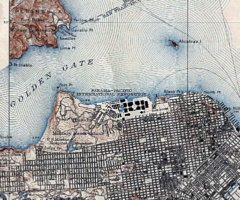
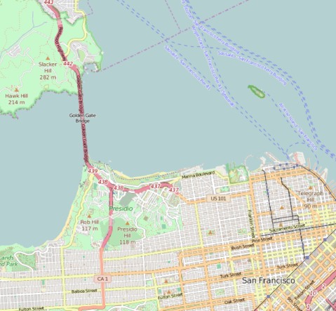
Road network algorithms are an important topic of study in Geographic Information Systems (GIS), in that road networks facilitate transportation and are the products of social, geographic, economic, and political forces. In addition, road networks are interesting data types, in that they combine both geometric information and graph-theoretic information. (E.g., see [4].) Formally, we view a road networks as a graph, where we create a vertex for every road intersection or major jog, and we create an edge for every pair of such vertices that have a road segment that joins them. In addition, some road networks are annotated with geometric/geographic information, such as the GPS coordinates of some vertices or labels identifying road names. Nevertheless, because road networks may contain many vertices and edges without such geometric/geographic information, we are interested in this paper in studying road networks from strictly a topological viewpoint, that is, as embedded graphs. Specifically, we are interested in the problem of determining how road networks evolve over time, e.g., highlighting places where new roads and bridges are added and where old roads and bridges are removed. (See Figure 1.)

Figure 1: A map of San Francisco from 1915 and one from 2016 (taken from OpenStreetMap). The top image is in the public domain; the bottom image is licensed under the Open Database License, CC BY-SA. Note that most of the roads in both maps are not labeled.

1.1 Problem Definition

Viewed topologically in terms of their graph properties, road networks are embedded graphs, that is, the edges incident on each vertex are given in a particular order (i.e., clockwise or counterclockwise), which defines a topological structure for the graph known as a rotation system (e.g., see [15]). Road networks are not typically planar graphs (e.g., see [4]), however, since there are edge crossings, for example, at overpasses. Thus, we cannot in general apply algorithms for planar graphs to road networks. Nevertheless, the vertices in road networks have bounded degrees (since the number of roads that meet at a single junction cannot be arbitrarily large); hence, a road network with $n$ vertices has $O(n)$ edges.

Given two undirected graphs, $G_{1}$ and $G_{2}$, an isomorphism of $G_{1}$ and $G_{2}$ is a bijection, $f$, from the vertices of $G_{1}$ to the vertices of $G_{2}$ such that $(u,v)$ is an edge in $G_{1}$ if and only if $(f(u),f(w))$ is an edge in $G_{2}$ (e.g., see [10]). In the subgraph isomorphism problem, we are given two graphs, $G_{1}$ and $G_{2}$, and asked to determine whether there is a subgraph of $G_{1}$ isomorphic to $G_{2}$. This problem is NP-complete, even if $G_{1}$ is an embedded planar graph, by a reduction from the planar Hamiltonian circuit problem [6]. Thus, defining the best matching between two road networks simply in terms of a maximum common subgraph is unlikely to lead to a polynomial-time algorithm. So let us restrict the types of matchings we consider.

Suppose we are given a subgraph, $G_{1}^{\prime}$, of a graph, $G_{1}$, and a subgraph, $G_{2}^{\prime}$ of a graph, $G_{2}$, such that $G_{1}$ and $G_{2}$ are embedded graphs, i.e., having specified rotation systems. Suppose further that $f$ is an isomorphism from $G_{1}^{\prime}$ to $G_{2}^{\prime}$. We say that $f$ is conformal if it satisfies the following conditions:

1. For every vertex $v$ in $G_{1}^{\prime}$, $v$ has the same degree in $G_{1}$ as $f(v)$ has in $G_{2}$. That is, we only match vertices having the same degree.

2. For every pair of incident edges, $(v,u)$ and $(v,w)$, in $G_{1}^{\prime}$, $(v,u)$ precedes $(v,w)$ in the clockwise order of edges around $v$ in $G_{1}$ if and only if $(f(v),f(u))$ precedes $(f(v),f(w))$ in the clockwise order of edges around $f(v)$ in $G_{2}$. That is, we match vertices consistently with the edge orderings around each vertex.

Since road evolution tends to involve adding or removing whole roads or neighborhoods, we restrict our notion of road network evolution in this paper to be defined in terms conformal matchings. There is still one more restriction that we need to add, however, which deals with degeneracies that are unlikely to occur in real-world road networks.

Suppose we are given two road networks, $G_{1}$ and $G_{2}$, and a maximum-cardinality subgraph, $G_{1}^{\prime}$, having a conformal matching, $f$, to a subgraph of $G_{2}$ (which is how we determine the parts of $G_{1}$ that are the same in $G_{2}$). We say that $G_{1}$ and $G_{2}$ are degenerate if, for any vertex $v$ in $G_{1}^{\prime}$ and edge $(v,w)$ in $G_{1}$, we can change the assignment, $f(w)$, for $w$ and still have $f$ be a conformal matching (even allowing for $f(w)$ to be undefined). Since our intended applications involve the second road network being a newer copy of the first, a maximum-cardinality subgraph with a conformal matching identifies the portions of the road network that have not changed over time; hence, the portions outside of this maximum-cardinality subgraph identify the portions that have changed. Thus, we argue that such applications involve non-degenerate graphs, since it is unlikely, for example, for us to encounter an $8\times 16$ grid that evolves into a grid-like annulus of 64 nodes with radius 8, which would be degenerate. Given that such configurations are likely to be rare in the real world, we are interested in this paper only in finding maximum conformal matchings in non-degenerate pairs of road networks, which is a problem we refer to as the map evolution problem.

Incidentally, the map evolution problem should not be confused with the map matching problem (e.g., see [8, 9]), which is the unrelated problem of matching a trajectory of (possibly noisy) GPS coordinates, as might be produced by a moving vehicle, to the geometry of the road network in which the trajectory is traveling.

1.2 Prior Related Work

As noted above, the map evolution problem is related to the graph isomorphism problem, which has a rich history (e.g., see [7, 10]), due to the fact that it is not known to be NP-complete, and the best known worst-case algorithm runs in quasipolynomial time [2], but the problem tends to be feasible in practice (e.g., see [10]). For the generalized approximate graph isomorphism problem, which is NP-hard, Arvind et al. [1] give a quasipolynomial approximation algorithm. Such algorithms are necessarily not taking advantage of any efficiencies, however, that could come from topological considerations like our restrictions to embedded graphs and conformal matchings.

The map evolution problem is also related to the map alignment problem, which is also known as GIS conflation (e.g., see [11, 12]). In this problem, one is given two road networks, including both topological information (such as vertex-edge-face relationships) and geometric information (such as vertex coordinates and edge directions and lengths), and one is interested in computing a “most likely” matching between the two networks. Rosen and Saalfeld [11, 12] develop an iterative process involving a human operator based on matchings that use topology/geometry classifications of the vertices, edges, and faces of the maps. Xiong [19] extends these topological/geometric approaches using more sophisticated classifications. Savary and Zeitouni [13] and Zhang [20] extends these approaches further by including additional properties, such as geographic data, including road names and shapes. Their use of geometry, however, implies that all of these conflation methods are not strictly topological algorithms and their performance degrades when roads or vertices lack geometric or geographic information.

Detecting changes in road networks and geographic regions has also been studied from the perspective of image processing, e.g., using satellite images (e.g., see [18]). For example, Zhang and Couloigner [21] use image analysis to extract polylines defining roads and match them between two images of the same geographic region taken at different times. Such image-analysis approaches are inherently geometric, however; hence these are also not strictly topological algorithms and do not apply when image data is not available.

Our topological approach is more closely aligned with the work of Eppstein et al. [5], which uses a topological approach for approximately matching for quadrilateral meshes used in computer-generated animations. Our approach differs from their methods, however, in that we do not consider faces in our matching algorithm (since road network faces can be large and complex), whereas their method crucially depends on matching faces (which in their application are always quadrilaterals or triangles).

1.3 Our Results

In this paper, we study the map evolution problem, for matching two road network graph of same area but from different time, by using only topological properties. The primary motivation for this approach is to show that the map evolution problem problem can be solved effectively using only topological information. Thus, this gives GIS practitioners a tool that can be applied for solving the map evolution problem even for problem instances where geometric and geographic information is missing, such as in older hand-drawn maps, pairs of maps where only one of them is derived from an image, pairs of maps annotated in different languages, or maps missing geographic and geometric annotations due to scaling resolution.

We develop an algorithm for the map evolution problem that runs in polynomial time for finding conformal matchings between non-degenerate embedded graphs, such as real-world road networks. Our algorithm uses a breadth-first flooding technique that begins each flooding phase by finding potentially-matching “seed” vertices using a labeling technique similar to that used in the the Weisfeiler-Leman (WL) graph isomorphism algorithm (e.g., see [7]). So as to limit the amount of flooding done in subgraphs that ultimately are determined not to match, our algorithm is probabilistic in nature—when we don’t have any pair of unique starting nodes, we take the pair which minimizes an estimate of the probability of a wrong match. We provide verification of our algorithm in experiments and case studies that show empirically that our algorithm produces good matches in practice.

2 Our Algorithm

In this section, we describe our topological algorithm for finding a best conformal matching between two non-degenerate road networks, $G_{1}$ and $G_{2}$:

1. Create quasi-unique labels for each vertex, $v$, in $G_{1}$ and $G_{2}$ based on the degrees of the nodes at distance at most $k$ from $v$, for an input parameter, $k$. (We show in our experimental section that choosing $k$ between 5 and 8 tends to give the best results.)

2. Choose a good pair of starting nodes, $s_{1}\in G_{1}$ and $s_{2}\in G_{2}$, with the same quasi-unique label, $L$, and, for each such pair having label $L$, perform the following:

   1. Perform a breadth-first search (BFS) matching of the corresponding portions in $G_{1}$ and $G_{2}$ that are respectively reachable from $s_{1}$ and $s_{2}$ according to a greedy conformal matching that emanates out from these starting nodes.

   2. Save this conformal matching that starts from $s_{1}$ and $s_{2}$ if it is the best (highest cardinality) such matching found so far for this quasi-unique label.

3. Commit the conformal matching that began with $s_{1}$ and $s_{2}$, removing all matched nodes as candidates for starting nodes.

4. Repeat the above process for another good pair of starting nodes, if such a pair of nodes still remains.

We describe these steps in more detail below.

2.1 Labeling Vertices

The first step of our algorithm is to give each vertex, $v$, in $G_{1}$ and $G_{2}$ a quasi-unique label, based on the degrees of the nodes at distance at most $k$ from $v$, for a given parameter, $k$. This approach is similar to a labeling method used in the (exact) graph isomorphism algorithm by Weisfeiler and Leman (WL) [7]. Specifically, we begin by determining the degree, deg$(v)$, of each vertex, $v$. Then we create a list for each vertex, $v$, which contains its degree, followed by the degrees of nodes at distance $1$ from $v$, nodes at distance $2$ from $v$, and so on, up to a distance $k$, where $k$ is an input parameter for this step. So as to make sure that these labels are quasi-unique, we add the degrees of these nodes at distance at most $k$ from $v$ according to a canonical ordering, which in our case is a lexicographically minimum breadth-first search (BFS) ordering. This BFS ordering sorts the immediate neighbors of $v$ according to a lexicographically minimum cyclic ordering of $v$’s neighbors based on their degrees, and then it performs a BFS from this queue, adding nodes to the queue based on the cyclic ordering of edges around each vertex so long as they are at distance at most $k$ from $v$.

We return a dictionary for $G_{i}$ (for $i=1,2$), which we call masterTable$({G_{i}})$, such that each entry in this dictionary is a list of vertices having the same quasi-unique label. That is, the keys we use to index the (list) entries in masterTable$({G_{i}})$ are the label$[v]$ lists produced by our quasi-labeling method.

The pseudocode for this step is given in Algorithm 1.

function labelNodes$(k,G)$;

for each $v\in G$ do

       label[$v$] = (deg$(v)$)        # label is a list;

       for $u\in\mbox{lexicographicBFS}(v,k)$ do

             Append deg($u$) to end of label[$v$];

            

       end for

      Add $v$ to masterTable$(G)\,$[label$[v]]$;

      

end for

Algorithm 1 Algorithm for labeling each vertex with a quasi-unique label. The method, lexicographicBFS$(v,k)$, returns an ordered list of nodes as would be visited a breadth-first search (BFS) from $v$, starting with the neighbors of $v$ enqueued according to a lexicographically minimum cyclic ordering of $v$’s neighbors based on their degrees. This BFS explores all nodes at distance at most $k$ from $v$.

With respect to the efficiency for performing this step, note that the time needed for this step is dominated by our doing a BFS from each node, $v$, to explore those other nodes at distance $k$ from $v$. Since the vertices of a road network have degree bounded by some parameter, $d$, this step takes worst-case time $O(d^{k}n)$, for a road network of $n$ nodes. In practice, $k$ is a constant, $d$ is usually $3$ or $4$, and the graph is rather sparse; hence, this step runs in $O(n)$ time in practice.

2.2 Choosing Pairs of Starting Nodes

After we have labeled each vertex of $G_{1}$ and $G_{2}$ with quasi-unique labels, we need to choose a pair of starting nodes in $G_{1}$ and $G_{2}$ with the same label to start the matching process. If we are able to find a unique pair of nodes having the same label, then we can take them as starting nodes and start our matching. But it may happen that we don’t have any such unique pair of nodes; that is, it might be the case that there are at least $3$ nodes from $G_{1}\cup G_{2}$ for each quasi-unique label of vertices in the master table.

For each distinct label, $L$, let $n_{1}(L)$ denote the number of vertices in $G_{1}$ with label $L$ and let $n_{2}(L)$ denote the number of vertices in $G_{2}$ with label $L$. As mentioned above, if we have a label, $L$, such that $n_{1}(L)=n_{2}(L)=1$, then we choose the unique pair of vertices, $s_{1}\in G_{1}$ and $s_{2}\in G_{2}$, with label $L$ as a good pair of starting vertices.

Otherwise, we would like to choose a pair, $s_{1}\in G_{1}$ and $s_{2}\in G_{2}$, that maximizes the probability that there is a large conformal matching of the connected components of $G_{1}$ and $G_{2}$ respectively containing $s_{1}$ and $s_{2}$, such that $s_{1}$ and $s_{2}$ have the same quasi-unique label, $L$. For any such label, $L$, the number of such candidate pairs is $n_{1}(L)\cdot n_{2}(L)$; hence, to maximize the probability of finding a good pair of starting nodes, we choose a pair, $s_{1}$ and $s_{2}$, that minimizes the product, $n_{1}(L)\cdot n_{2}(L)$, since the probability such a pair actually correspond to corresponding nodes in $G_{1}$ and $G_{2}$, conditioned on their having the same label, $L$, is at least $1/(n_{1}(L)\cdot n_{2}(L))$.

We then perform a flooding-based search from each such $s_{1}$ and $s_{2}$ with label $L$, committing to the pairing that results in the largest matched components in $G_{1}$ and $G_{2}$. Then, we remove all the matched vertices in $G_{1}$ and $G_{2}$ from consideration (since they are now matched), and we repeat our search for another good pair of starting seed vertices.

In order to perform such searches and updates quickly, we use an auxiliary priority queue data structure that stores each quasi-unique label, $L$, according to its priority, $n_{1}(L)\cdot n_{2}(L)$. Such products can be found by taking the product of lengths of both lists for each label used as a key in masterTable. As we are performing our greedy matching processes, we also need to update these lists by removing each matched pair of nodes. Of course, this will also change the product for each label, so we have to update labels in our priority queue to now have new priorities. Since these products are always integers in the range $[1,C]$, for some parameter, $C\leq n^{2}$, let us use a van Emde Boas tree [16, 17] (vebTree) for storing non-zero products, $n_{1}(L)\cdot n_{2}(L)$, for each label, $L$, as well as a hash table, productTable, that gives us the product for any existing label, $L$. This allows us to perform searches, updates, and finding of labels with minimal product values in $O(\log\log C)$ time.

Every time the algorithm needs a pair of starting nodes, it finds a label, $L$, with minimum product, $n_{1}(L)\cdot n_{2}(L)$, from vebTree. If there are multiple labels having that product, we randomly choose any one of them. After finding the required label, we take a pair of nodes having the same label from the masterTable. After finding the starting pair of nodes, we update these data structures, and the productTable, so that we don’t consider this pair of nodes again. Note this approach works even when we have unique pair of nodes having the same label. In that scenario, the product will be $1$ and that will be minimum product in vebTree.

With respect to efficiency, we can do all the setup for this step in $O(n\log\log C)$ time. Moreover, we can determine already at this point what is the maximum product, $n_{1}(L)\cdot n_{2}(L)$, over all labels, $L$, for a given value of $k$. Since $k$ is a constant for real-world road networks and there is an inverse relationship between $k$ and the size of these products, we can perform a (binary) search to choose $k$ so that the maximum product size is bounded by some constant, $C$. The running time of this search would be $O(n)$ for constants $k$ and $C$.

There is a tradeoff, however, between using a large value for $k$ and getting good matches, since two starting nodes are paired only if their quasi-unique labels are the same, that is, if the respective portions of the road network at distance $k$ from these nodes is the same. Since we are considering road networks that are evolving, we therefore don’t want to set too high a value for $k$. Thus, we would like to choose $k$ as small as possible so that the products, $n_{1}(L)\cdot n_{2}(L)$, are bounded by a constant, $C$. (Say, $C\leq 24$.) As we note in the experimental section of this paper, choosing $k$ between 5 and 8 seems to work well in practice for this purpose.

2.3 Flood-based Conformal Matching

After finding a starting pair of nodes, we start our greedy BFS matching process. We begin by marking the starting nodes as matched and we add them to our current tentative matching. As we perform our BFS matching process, we will tentatively be matching up additional pairs of nodes from $G_{1}$ and $G_{2}$, updating our supporting data structures as we go, e.g., to tentatively remove each such pair from consideration in vebTree. Moreover, if a starting node has more than one lexicographically minimum ordering of the degrees of its neighbors, then we also consider each such ordering of the edges, performing our BFS matching process for each. Tentative matchings are compared on the basis of number of matched nodes and the matching with maximum number of matched nodes is taken as best matching.

This raises an important implementation detail, which we should probably discuss before going on to other details. Our matching algorithm considers different pairs of starting vertices (and even possibly different starting orientations of their incident edges), looking for the pair that produces the largest portions of matching subgraphs. Thus, we may have tentative matches that need to be undone so that other tentative matches can be considered.

There are at least two possible ways to deal with this branch-and-bound element in our conformal matching algorithm. One way is to checkpoint our supporting data structures, like vebTree, masterTable, and productTable, saving the version that produced the best tentative match so far. This is the method we use, for example, in the version of our algorithm that we implemented for our experiments, since it is easy to implement. Another way is to perform a two-phase commit, where we perform updates to global copies of these data structures, but keep a history of the updates we have performed during a tentative matching, so that we can then roll back these updates if we do not commit to that tentative matching (because there is another one that gave a larger number of matched vertices). This is the version of our algorithm that we analyze for our theoretical analysis.

Given that there is some method that allows us to roll back to an earlier state of our supporting data structures, vebTree, masterTable, and productTable, let us discuss in more detail how our conformal BFS proceeds.

Once we map the neighbors around a pair of starting nodes, as discussed above, we flood-search both graphs using a conformal-matching BFS. When we reach any other node except a starting node in the flooding, we know the edge we are coming from and as we are following clocking ordering around any node, there will be exactly one ordering around that node in which we can traverse and map the neighbors with another graph, so as to be forming a conformal matching. Figure 2 shows an example.

[] []

Figure 2: Neighbor ordering around a degree-$4$ node, $v_{1}$, and its matching node, $v_{2}$. In this example, node 1 in $G_{1}$ matches with node 1 in $G_{2}$, and we know that the we reached the matched nodes $v_{1}$ and $v_{2}$ through the respective nodes, $1$, so now their clockwise ordering is fixed and the mapping of neighbors will be $(4,7),(3,6),(2,5)$.

For matching any two nodes, $v_{1}\in G_{1}$ and $v_{2}\in G_{2}$, that are not starting nodes, they should satisfy following properties:

• both $v_{1}$ and $v_{2}$ should be unmatched.

• degree of $v_{1}$ should be same as $v_{2}$.

If any of these two conditions fail, we don’t match $v_{1}$ and $v_{2}$ and we terminate that branch of the BFS. If both the conditions are satisfied, then we mark $v_{1}$ and $v_{2}$ as matched, add them to current matching and the queue for the BFS. Then we remove them from masterTable, vebTree and productTable, so that they are not considered again in the matching process. The pseudocode for this step in our algorithm is given as Algorithm 2.

function processNodes($u_{1},u_{2}$);

add ($u_{1}$, $u_{2}$) to matching;

mark $u_{1}$ and $u_{2}$ as matched;

add corresponding neighbors of $u_{1}$ and $u_{2}$ to bfsQueue;

update masterTable, vebTree and productTable to remove $u_{1}$ and $u_{2}$;

Algorithm 2 Algorithm to process nodes in BFS.

When there is no further branch that can be matched, our BFS search terminates. If this is the best tentative matching for the given quasi-unique label, $L$, then we tentatively save the matching corresponding to this BFS to the total matching. Then we check if there is still any remaining pair of seed nodes having this same label. If so, then we perform another conformal BFS for this next pair of seed vertices. Once we have completed performing a tentative matching for each pair of seed nodes having the same quasi-unique label, $L$, we commit to the matching for this label that produced the largest match.

Then we check if vebTree is empty or not. If vebTree is empty, we terminate the algorithm and return the total matching. If not, we repeat our search for a quasi-unique label, $L$, having the smallest product, $n_{1}(L)\cdot n_{2}(L)$, and repeat the above conformal BFS for that label.

The pseudocode for this step in our algorithm is given as Algorithm 3.

function matching(masterTable,$G_{1},G_{2}$);

create prodTable and vebTree;

totalMatching = [ ];

while vebTree is not empty do

       minProd = vebTree.min$()$;

       startingLabel = productTable[minProd];

       startingPairs = (masterTable$(G_{1})\,$[startingLabel], masterTable$(G_{2})\,$[startingLabel]);

       find all mappings of neighbors around each pair in startingPairs;

       for each of the mappings in a startingPair do

             matching = [ ];

             $(s_{1},s_{2})$ = this instance of startingPair[0],startingPair[1];

             bfsQueue = $()$;

             processNodes($s_{1}$,$s_{2}$);

             while bfsQueue is not empty do

                   $v_{1},v_{2}$ = pop(bfsQueue);

                   if $v_{1}$ and $v_{2}$ are both unmatched then

                         if deg$(v_{1})$ = $deg(v_{2})$ then

                               processNodes($v_{1}$,$v_{2}$);

                              

                         end if

                        

                   end if

                  

             end while

            checkpoint this matching if it’s best for this startingPair;

            

       end for

      add the best matching found to totalMatching;

      

end while

Algorithm 3 Our flood-based conformal matching algorithm.

Each time we explore subgraphs of $G_{1}$ and $G_{2}$ for a particular starting pair, $s_{1}$ and $s_{2}$, that are in the starting label set of pairs for some quasi-unique label, $L$, and one of the deg$(s_{1})$ possible orientations of edges, we traverse subgraphs of some size at most, $n(L)\leq n$, where $n(L)$ is the size of the largest match for the label $L$. Thus, the running time of this part of our algorithm is at most $O(n(L)\log\log C)$, where $C$ is the maximum value of a product, $n_{1}(L^{\prime})\cdot n_{2}(L^{\prime})$, for some label, $L^{\prime}$. If $d$ is the maximum degree in a road network (e.g., $d\leq 8$), then the total worst-case running time of our BFS matching algorithm is therefore

$$O\left(dC\sum_{L}n(L)\log\log C\right)=O(dCn\log\log C),$$

since $\sum_{L}n(L)\leq n$, because the maximum amount of nodes we can ultimately match in a pair of non-degenerate road networks is $n$. Combining this with the theoretical analysis of the other steps in our matching algorithm implies that the total running time of our entire algorithm is $O(d^{k}n+dCn\log\log C)$, where $d$ is the maximum degree of a road network, $k$ is the distance we choose for producing quasi-unique labels, and $C$ is the maximum value of a product, $n_{1}(L)\cdot n_{2}(L)$, for any label, $L$. Thus, in the practical case when $d$, $k$, and $C$ are constants, our matching algorithm runs in $O(n)$ time.

(a) $k=1$

(b) $k=5$

Figure 3: Histogram plots for Amador County, CA from 2000 to 2006.

(a) $k=1$

(b) $k=7$

Figure 4: Histogram plots for Alameda County, CA from 2000 to 2006.

3 Experiments

In this section, we provide an empirical evaluation of our topological flood-based matching. All of our experiments were ran on data from the U.S. TIGER/Line road network database [3].

3.1 Preprocessing the Data

The TIGER/Line database provides the road networks in two different file formats: shapefile and TIGER/Line ASCII format. The data the shapefile format provides allows a graph to be created that not only has a node for every intersection of two roads, but also nodes to indicate the curvature of a road. That is, the format allows for curved roads to be represented as a sequence of many two-degree vertices. Therefore, for the preprocessing of files in the shapefile format, we simply take the first and the last vertex for each road to avoid introducing unnecessary two-degree vertices. With this approach to processing files in the shapefile format and fact that the TIGER/Line ASCII format lends itself to easy conversion to the definition of a road network given in the introduction, our algorithm performs well on both file formats.

3.2 Tuning the Seed-labeling Parameter

Let us consider the choice of the value for $k$, the parameter that is input to Algorithm 1 that defines distance to which to perform a lexicographic BFS so as to improve the uniqueness of vertex labels. To characterize this uniqueness factor, let us define the approximation ratio of a labeling as $a/b$, where $a$ is the number of pairs of nodes with the same label and $b$ is the minimum of the number of nodes in the two graphs. Intuitively, if $k$ is small, there will likely be many pairs of nodes $(u,v)$ with $u$ in $G_{1}$ and $v$ in $G_{2}$ that both have label $L$ where $n_{1}(L)\cdot n_{2}(L)$ is large. For example, labels like “44444", which indicates a four-way intersection that leads to four other four-way intersections, are likely to be common, and many other examples like this are likely from real-world. As many of these products are expected to be large, we would expect the approximation ratio to be larger for smaller value for $k$, because we could be possibly finding many pairs of vertices with the same label that should not actually be matched. For instance, we might find two vertices labeled “44444" even though they are not similar beyond their immediate neighbors. We expect to run into this situation only when the product is large since our algorithm matches the pair of vertices for a given label that maximizes the number of nodes matched.

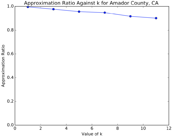
As we increase the value of $k$, we would expect that the approximation ratio to decrease. That is, if $k$ is large, we expect there to be more labels $L^{\prime}$ such that $n_{1}(L^{\prime})\cdot n_{2}(L^{\prime})$ is small or even 1, as the labels should become more distinct as $k$ increases. Because the labels are expected to be more distinct in this case, it should be less likely to find pairs of vertices with those labels, causing the approximation ratio to decrease.

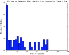
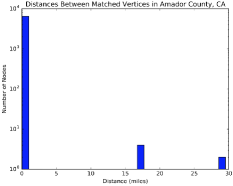
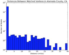
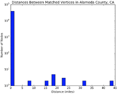
The histograms in Figures 3 and 4 exemplify the preceding interpretation of the parameter $k$. The $x$-axis indicates the physical distance between every node and its pair partner(s) with the same quasi-unique label, $L$, using the longitude and latitude values given from the database. The distance is determined using the haversine formula, which yields the shortest distance between two points on a sphere [14]. (Although our algorithm doesn’t use geometric information to determine matching pairs, we used geometric information in this experiment to empirically validate our approach.) Ideally, all pairs should be at distance 0 from each other.

As we expected, larger $k$ values minimize the physical distances between pairs of nodes with the same label, which gives us a more accurate matching; hence, it reduces the number of false pairs that our algorithm needs to consider. A histogram that is highly skewed is desirable, as that implies that the number of incorrect nodes being falsely matched is small. Note that the Amador County data from 2000 and 2006 in Figure 3 included 6,970 and 6,784 nodes, respectively, and the Alameda County data from 2000 and 2006 in Figure 4 included 52,566 and 51,054 nodes, respectively.

Figure 5 shows the change of the approximation ratio with respect to the change in $k$ for Amador County. The decrease in the approximation ratio with the increase in $k$ again matched our intuition. The plot with the same $x$-axis and $y$-axis values for Alameda County started at a similar approximation ratio and decreased at a similar rate, so it was omitted.

Figure 5: Change in approximation ratio for Amador County, CA from 2000 to 2006

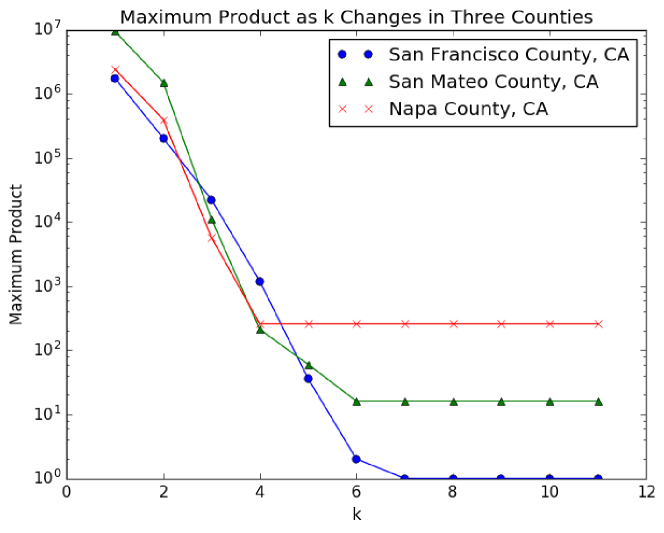
We also plot the change in the maximum product with respect to $k$ in Figure 6. As described in Section 2, the maximum product is the value $\max\{n_{1}(L)\cdot n_{2}(L):L\text{ is a label generated by Algorithm~{}\ref{alg:find_seed}}\}$. As expected, the maximum product decreases as $k$ increases. Note that only for San Francisco County does the maximum product reach 1. This is due to the fact that for the other counties, there are labels that do not change as $k$ increases as the nodes the labels correspond to are in small connected components e.g. “121" is the cause of this in San Mateo County.

Figure 6: Change in maximum product for Napa, San Francisco, and San Mateo Counties with road networks from 2000 and 2006

3.3 Example Output of Our Algorithm

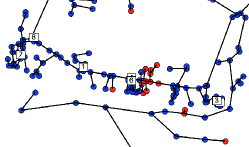
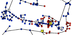
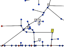
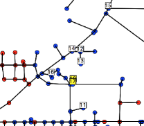
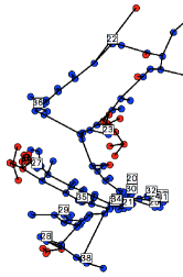
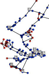
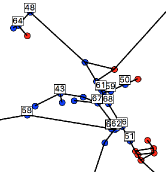
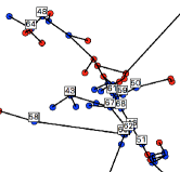
In this subsection, we provide a visualization of the matching our algorithm created for Del Norte County, CA. We performed the matching with $k=3$ and then took four snapshots of the matching to enlarge the details. For Figures 7, 8, 9, and 10, a node is colored blue if it was matched and red otherwise. Furthermore, a node with a white box above it from the first image containing number $i$ matches the node with a white box above it containing the number $i$ from the second image.

First, consider Figure 7. Solely based off of geographic location, it is clear that the nodes are being matched to the correct area. After further inspection, it can be seen that the graph has remained nearly the same around the white boxes containing “1", “3", “7", and “8". Near each of these white boxes, our matching algorithm has matched the correct nodes, indicated by all of the blue nodes surrounding said boxes. Figure 7 also demonstrates the issue of using a small value for $k$. The yellow boxes in Figure 7b indicate nodes that have been matched to other nodes in the graph from Figure 7a that are not included in the image. This incorrect matching is due to the fact that when $k$ is small, as mentioned earlier, it is likely that many nodes will end up with the same label, yielding a higher likelihood of incorrectly matching two nodes that should not be matched.

Second, consider Figure 8. The white boxes in these figures are here to indicate that the matching algorithm is performing properly in many parts of the graph. As we are just using topological features, we also get some unexpected matching as shown in Figure 8. The two yellow boxes in Figure 8a are matched to the two yellows boxes in Figure 8b. A new vertex was added in the 2006 graph that caused the matching of the vertices under the yellow boxes to occur in the wrong place. Because we are only using topological features, our matching algorithm cannot distinguish between the new vertex and the old one that it should be matching to.

Last, consider Figures 9 and 10. Many more white boxes were included to show the success of our matching algorithm in these portions of the graph.

(a) $2000$

(b) $2006$

Figure 7: First example of a portion of a matching for Del Norte County, CA where $k=3$.

(a) $2000$

(b) $2006$

Figure 8: Second example of a portion of a matching for Del Norte County, CA where $k=3$

(a) $2000$

(b) $2006$

Figure 9: Third example of a portion of a matching for Del Norte County, CA where $k=3$.

(a) $2000$

(b) $2006$

Figure 10: Fourth example of a portion of a matching for Del Norte County, CA where $k=3$.

3.4 Detailed Analysis

We ran our algorithm on $40$ different counties in California ranging from small counties to big counties. The results for our experiments are shown in Table 1. Each row gives analysis about one particular county where $G_{1}$ is obtained from TIGER/Line ASCII format from the year $2000$ and $G_{2}$ is obtained from TIGER/Line ASCII format from the year $2006$. The column titled “seed time" indicates the time taken to find the seed vertices for the given value of $k$ and the column titled “match time" indicates the amount of time taken for the topological flood-based matching algorithm. We ran the experiments on a machine with $3.1$ GHz Intel Core i7 CPU and $16$ GB of RAM and report the timings in seconds. The last column titled “thresh. ratio" is the ratio of number of pairs of matched vertices within $5$ miles of each other to the total number of pairs of matched vertices which gives up the quality of matching. We can see from the table that thresh. ratio is always greater than $0.9$ which tells us that our algorithm performs well on all kinds of inputs.

Table 1: Results for various counties throughout California

county	$k$	nodes of $G_{1}$	nodes of $G_{2}$	edges of $G_{1}$	edges of $G_{2}$	seed time (seconds)	match time (seconds)	approx. ratio	thres. ratio
Alameda	9	40752	40242	67226	66644	778.544	7.686	0.9777	0.9997
Alpine	5	1448	1427	1838	1811	0.536	0.311	0.9439	0.9985
Amador	5	6970	6784	9198	8991	3.017	0.764	0.9553	0.9998
Butte	8	19856	21304	27896	29955	66.540	34.509	0.6878	0.9963
Calaveras	8	13770	13043	18141	17690	23.050	1.185	0.0400	0.9196
Colusa	5	5039	5700	7285	8589	4.231	8.106	0.8106	0.9867
Contra Costa	9	37148	36564	55555	54750	323.512	70.794	0.9482	0.9995
Del Norte	5	5383	7034	7386	9785	3.861	39.562	0.4811	0.9258
El Dorado	9	24248	24103	33331	33271	108.336	10.559	0.9766	0.9991
Fresno	9	51006	50614	83081	82640	744.009	346.011	0.9796	0.9992
Imperial	8	18104	18105	28716	28639	92.026	1.481	0.9592	1.0
Kings	8	11842	15328	18775	25521	87.083	7.071	0.3541	0.9978
Lake	8	12437	18500	17486	26176	47.485	391.934	0.1331	0.9553
Lassen	8	16216	19519	24024	28044	57.645	241.791	0.3804	0.9837
Madera	8	16936	16633	25164	24842	77.837	4.864	0.9633	0.9998
Marin	8	13733	13455	19722	19372	44.946	1.231	0.9446	1.0
Mariposa	5	9241	10538	12033	13830	4.558	119.975	0.5746	0.9546
Mendocino	9	22326	26153	30231	36142	107.554	403.188	0.3761	0.9901
Merced	8	16576	19619	25266	29568	78.726	9.331	0.6058	0.9940
Modoc	8	13304	17408	19674	24889	44.782	3.998	0.3229	0.9837
Mono	5	9159	11345	13203	16178	6.440	30.914	0.6179	0.9595
Monterey	9	31887	33831	48204	51313	324.838	350.278	0.7654	0.9978
Napa	5	6932	6827	10054	9867	4.813	19.717	0.9491	0.9933
Nevada	8	15903	15268	21729	20935	30.650	6.726	0.9135	0.9994
Placer	9	25365	25437	35603	35913	116.914	41.591	0.9287	0.9996
San Benito	5	7555	10311	10421	14649	5.801	30.310	0.5597	0.9503
San Francisco	5	9803	11570	20313	24218	20.241	0.977	0.7138	1.0
San Mateo	9	21571	21101	35132	34532	288.204	5.469	0.9666	0.9997
Santa Cruz	8	14374	14063	20545	20142	48.941	19.229	0.9694	0.9997
Shasta	9	25436	33824	35129	47588	163.593	431.638	0.1867	0.9732
Sierra	5	4809	6522	6603	8912	3.273	5.000	0.3559	0.8603
Siskiyou	9	28210	38150	39682	52616	140.771	705.416	0.1442	0.9528
Solano	8	15930	31249	24859	46954	106.300	63.848	0.1398	0.9654
Stanislaus	8	18254	19240	29327	31094	110.927	1.703	0.5786	0.9962
Sutter	5	6311	6164	9670	9494	4.293	0.319	0.9704	1.0
Tehama	8	15399	19177	21756	27353	53.793	13.337	0.3802	0.9844
Trinity	8	12042	11944	15501	15434	15.961	77.516	0.9780	0.9945
Tulare	9	27555	27302	42308	42257	269.419	10.146	0.9632	0.9993
Tuolumne	9	14830	17135	19985	23283	47.406	131.849	0.2621	0.9809
Yuba	5	9354	9267	13529	13407	5.791	4.158	0.9840	0.9995

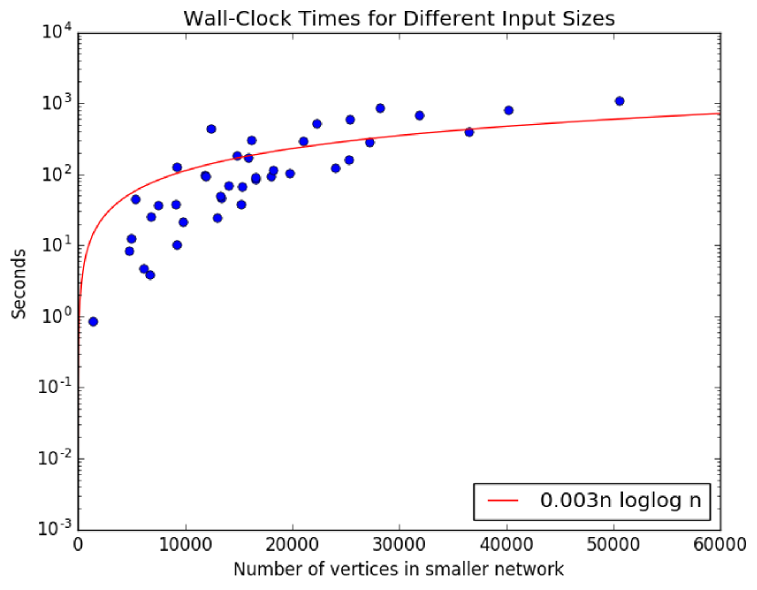
Figure 11 plots the experiments in Table 1 with the total running time (seed time plus match time) as the $y$-axis and the size of the smaller graph as the $x$-axis. The red line represents the function $0.003n\log\log n$. Therefore, it seems that the variable $C$ defined in Section 2 is much less than $n$, which is good for the running time of our algorithm.

Figure 11: Running times for our algorithm on the graphs given in Table 1

4 Conclusion

We have given a purely topological algorithm for determining the changes that occur between two road networks, and we have provided both theoretical and experimental analysis to show that our algorithm is effective and efficient. We therefore feel that this algorithm provides a good tool for solving the map evolution problem when geometric or geographic features are missing from one or both of the road networks being considered.

Acknowledgments

This article reports on work supported by the Defense Advanced Research Projects Agency under agreement no. AFRL FA8750-15-2-0092. The views expressed are those of the authors and do not reflect the official policy or position of the Department of Defense or the U.S. Government. This work was also supported in part by the U.S. National Science Foundation under grants 1228639 and 1526631. We would like to thank David Eppstein for several helpful discussions related to the topics of this paper.

References

- [1] V. Arvind, J. Köbler, S. Kuhnert, and Y. Vasudev. Approximate graph isomorphism. In B. Rovan, V. Sassone, and P. Widmayer, editors, 37th Symp. on Mathematical Foundations of Computer Science (MFCS), pages 100–111, 2012.
- [2] L. Babai. Graph isomorphism in quasipolynomial time. arXiv preprint arXiv:1512.03547, 2015.
- [3] U. S. Census Bureau. Tiger/line shapefiles and tiger/line files. https://www.census.gov/geo/maps-data/data/tiger-line.html.
- [4] D. Eppstein and M. T. Goodrich. Studying (non-planar) road networks through an algorithmic lens. In ACM Conf. on Geographic Information Systems (GIS), pages 16:1–16:10, 2008.
- [5] D. Eppstein, M. T. Goodrich, E. Kim, and R. Tamstorf. Approximate topological matching of quad meshes. The Visual Computer, 25(8):771–783, 2009.
- [6] M. R. Garey, D. S. Johnson, and R. E. Tarjan. The planar hamiltonian circuit problem is NP-complete. SIAM Journal on Computing, 5(4):704–714, 1976.
- [7] M. Grohe. Isomorphism testing for embeddable graphs through definability. In 32nd ACM Symp. on Theory of Computing (STOC), pages 63–72, 2000.
- [8] K. Liu, Y. Li, F. He, J. Xu, and Z. Ding. Effective map-matching on the most simplified road network. In ACM Conf. on Geographic Information Systems (GIS), pages 609–612, 2012.
- [9] Y. Lou, C. Zhang, Y. Zheng, X. Xie, W. Wang, and Y. Huang. Map-matching for low-sampling-rate gps trajectories. In ACM Conf. on Geographic Information Systems (GIS), pages 352–361, 2009.
- [10] B. D. McKay and A. Piperno. Practical graph isomorphism, II. Journal of Symbolic Computation, 60:94–112, 2014.
- [11] B. Rosen and A. Saalfeld. Match criteria for automatic alignment. In 7th Symp. on Computer-Assisted Cartography (Auto-Carto), pages 1–20, 1985.
- [12] A. Saalfeld. Conflation automated map compilation. International Journal of Geographical Information System, 2(3):217–228, 1988.
- [13] L. Savary and K. Zeitouni. Automated linear geometric conflation for spatial data warehouse integration process. In 8th AGILE Conference on GIScience, 2005.
- [14] B. Shumaker and R. Sinnott. Astronomical computing: 1. computing under the open sky. 2. virtues of the haversine. Sky and Telescope, 68:158–159, 1984.
- [15] S. Stahl. The embeddings of a graph – a survey. Journal of Graph Theory, 2(4):275–298, 1978.
- [16] P. van Emde Boas. Preserving order in a forest in less than logarithmic time and linear space. Information Processing Letters, 6(3):80–82, 1977.
- [17] P. van Emde Boas, R. Kaas, and E. Zijlstra. Design and implementation of an efficient priority queue. Mathematical systems theory, 10(1):99–127, 1976.
- [18] A. Ventura, A. Rampini, and R. Schettini. Image registration by recognition of corresponding structures. IEEE Trans. on Geoscience and Remote Sensing, 28(3):305–314, 1990.
- [19] D. Xiong. A three-stage computational approach to network matching. Transportation Research Part C: Emerging Technologies, 8(1):71–89, 2000.
- [20] M. Zhang. Methods and implementations of road-network matching. PhD thesis, Technical University of Munich, 2009.
- [21] Q. Zhang and I. Couloigner. Automatic road change detection and GIS updating from high spatial remotely-sensed imagery. Geo-Spatial Information Science, 7(2):89–95, 2004.