Liquid water through density-functional molecular dynamics: Plane-wave vs. atomic-orbital basis sets

Abstract

We determine and compare structural, dynamical, and electronic properties of liquid water at near ambient conditions through density-functional molecular dynamics simulations, when using either plane-wave or atomic-orbital basis sets. In both frameworks, the electronic structure and the atomic forces are self-consistently determined within the same theoretical scheme based on a nonlocal density functional accounting for van der Waals interactions. The overall properties of liquid water achieved within the two frameworks are in excellent agreement with each other. Thus, our study supports that implementations with plane-wave or atomic-orbital basis sets yield equivalent results and can be used indiscriminately in study of liquid water or aqueous solutions.

I Introduction

Liquid water plays a fundamental role in a multitude of phenomena of primary relevance to diverse areas of science. It is thus not surprising that in the past 30 years many efforts have been invested in better understanding liquid water properties at the molecular level. In this context, molecular dynamics and Monte Carlo simulation techniques have been largely employed as a complementary tool to experiment to investigate the nature of water at the atomic scale. Indeed, the increasing availability of computer resources and the improvement of computational algorithms have resulted in an accurate description of intermolecular interactions by the direct evaluation of the evolving electronic structure. In this respect, the Car-Parrinello methodCar and Parrinello (1985) has been instrumental to unify density functional calculations and molecular dynamics simulations in the study of liquid water.Laasonen et al. (1993); Sprik, Hutter, and Parrinello (1996) In fact, ab initio molecular dynamics simulations represent an invaluable tool to simultaneously access its structural, dynamical, Laasonen et al. (1993); Sprik, Hutter, and Parrinello (1996); Todorova et al. (2006); Lee and Tuckerman (2007); Schmidt et al. (2009); DiStasio Jr et al. (2014); Miceli, De Gironcoli, and Pasquarello (2015); Del Ben, Hutter, and VandeVondele (2015) and electronic Silvestrelli and Parrinello (1999); Prendergast, Grossman, and Galli (2005); Ambrosio, Miceli, and Pasquarello (2015); Chen et al. (2016) properties.

Most of the first-principles simulations of liquid water have been performed within the theoretical framework of density functional theory with a (semi)local approximation for the exchange-correlation energy.Laasonen et al. (1993); Sprik, Hutter, and Parrinello (1996); Lee and Tuckerman (2007) However, it has become clear that these approximations lead to a poor description of the structural and the dynamical properties. Liquid water is found to be overstructured, shows a very low diffusion coefficient, and its equilibrium mass density underestimates the experimental value by about 15%.Schmidt et al. (2009); Wang et al. (2011); Miceli, De Gironcoli, and Pasquarello (2015) These shortcomings still persist when the electronic structure is described at a higher level of theory, such as with hybrid density functionals. Todorova et al. (2006); Del Ben et al. (2013); Del Ben, Hutter, and VandeVondele (2015); Gaiduk, Gygi, and Galli (2015); Ambrosio, Miceli, and Pasquarello Similarly, from the more fundamental side, a quantum treatment of the nuclei slightly modifies the properties of the liquid. Morrone and Car (2008); Giberti et al. (2014); Del Ben, Hutter, and VandeVondele (2015) A substantial improvement is instead achieved when van der Waals interactions are correctly accounted for.Schmidt et al. (2009); Lin et al. (2009); Wang et al. (2011); Lin et al. (2012); Del Ben et al. (2013); DiStasio Jr et al. (2014); Miceli, De Gironcoli, and Pasquarello (2015); Gaiduk, Gygi, and Galli (2015); Del Ben, Hutter, and VandeVondele (2015); Ikeda and Boero (2015) For a broader overview on the performance of various popular exchange-correlation functionals in simulating liquid water, we refer the readers to the recent review by Gillan, Alfè, and Michaelides.Gillan, Alfè, and Michaelides (2016)

The need to perform accurate simulations of liquid water has brought the attention to post Hartree-Fock methods. Indeed, simulations of the liquid using sophisticated and accurate electronic-structure methods, such as the second-order Møller-Plesset approximation (MP2)Del Ben et al. (2013) and variational quantum Monte CarloZen et al. (2015) have been already reported in the literature. However, in spite of their accuracy, these methods are still computationally too demanding for a widespread use in routine simulations.

More recently, the need to accurately describe the electronic structure of liquid water has been constantly increasing. Indeed, this represents a major prerequisite for further progress in the design of new and efficient systems for photocatalytic water splitting.Grätzel (2001); Walter et al. (2010); Adriaanse et al. (2012); Ambrosio, Miceli, and Pasquarello (2015) To this aim, it has become imperative to resort to fully ab initio schemes which can shed light onto the electronic structure of the liquid without the use of any phenomenological parameters. In this respect, it has recently been shown that the combination of path-integral molecular dynamics simulations and quasiparticle self-consistent GW accounting for vertex corrections correctly reproduces the experimental photoemission spectrum.Chen et al. (2016)

It has become clear that a high level of theory is needed for an accurate description of liquid water. The scientific efforts in the last years have led to significant improvements of the available computer codes, which now allow for highly accurate simulations of liquid water. CP2K is one of the most versatile suite of programs used to perform atomistic simulations of solid-state, liquid, and biological systems.cp2 (2013) In CP2K, quantum chemistry simulations are performed in the framework of density functional theory relying on a mixed scheme based on Gaussian and plane-wave basis sets. Within this scheme, a wide variety of approximations for the exchange-correlation functional are implemented. The efficient use of basis sets and the availability of advanced algorithms, make of CP2K one of the most suitable and cost-effective codes for carrying out large scale first-principles simulations. Another largely used software suite to perform quantum chemistry and material science simulations is Quantum-Espresso.Giannozzi et al. (2009) Quantum-Espresso has specifically been designed to perform highly accurate electronic structure calculations. This accuracy rests on the use of plane-wave basis sets in conjunction with pseudopotentials. An important advantage of this scheme is the possibility of verifying the completeness of the adopted basis set by the adjustment of a single parameter corresponding to the kinetic energy cutoff of the plane waves. Furthermore, as shown in a recent community study, currently implemented pseudopotentials offer a high degree of accuracy and reproducibility with respect to all-electron calculations.Lejaeghere et al. (2016)

Most simulations on liquid water are currently performed with either atomic-orbital based codes such as CP2K or with plane-wave-based codes such as Quantum-Espresso. In doing so, the simulation parameters used in the two codes are set primarily on the basis of energy convergence criteria as they can be tested separately in the two codes. It is generally assumed that the adopted protocols lead to similar descriptions of the structural properties of liquid water,Kuo et al. (2004) but the comparison for the electronic and dynamical properties is not as well documented. Nevertheless, the agreement between different protocols is crucial for the general development of this research area and would indicate that the calculated properties are converged. In this respect, it is critical to compare simulations performed with identical exchange-correlation functionals and to adopt standard simulation parameters as currently in use in the research community. In particular, the use of the Car-Parrinello method is inappropriate for such a comparison as it could be biased by the use of a fictitious mass. Indeed, the use of fictitious masses are known to affect the detailed MD trajectoriesGrossman et al. (2004); Tangney and Scandolo (2002) and to be dependent on the adopted basis set.Car and Parrinello (1985)

In this work, we compare the results of first-principles molecular dynamics simulations of liquid water performed with the CP2K and the Quantum-Espresso codes, adopting standard simulation protocols separately set for the two codes. The molecular dynamics simulations in both the NVE and NpH ensembles are carried out within the Born-Oppenheimer approximation which does not present limitations that could be biased by the adopted basis set. In both cases, we use the same nonlocal exchange-correlation density functional which explicitly accounts for van der Waals interactions. Our results show that the two approaches are in excellent agreement with each other leading to an equivalent description of the structural, dynamical, and electronic properties of liquid water.

II Computational details

Throughout this work, the electronic structure and the atomic forces are calculated within the self-consistent Kohn-Sham approach to density functional theory (DFT). We perform simulations in which van der Waals interactions are explicitly taken into account. To this aim, among the several theoretical schemes proposed, we adopt the nonlocal rVV10 van der Waals functional.Sabatini, Gorni, and de Gironcoli (2013) This is essentially a revised but equivalent formulation of the VV10 nonlocal functional recently introduced by Vydrov and Van Voorhis.Vydrov and Van Voorhis (2010) Within this scheme, we use a semilocal exchange-correlation functional which results from a combination of the refitted Perdew-Wang exchange functionalMurray, Lee, and Langreth (2009) and the local density approximation to the correlation according to the Perdew-Wang parametrization.Perdew and Wang (1992) This semilocal exchange-correlation functional is then augmented with a nonlocal part which accounts for dispersion interactions. The result is a very simple analytic form which depends on an empirically determined parameter $b$, which controls the short-range behavior of the functional.Vydrov and Van Voorhis (2010); Sabatini, Gorni, and de Gironcoli (2013) This functional can be used to reproduce the correct physical properties of weakly bonded systems after an appropriate optimization of the $b$ parameter. For instance, the best description of the $S22$ set of molecules has been obtained for $b=6.3$.Sabatini, Gorni, and de Gironcoli (2013) However, while the binding energy and the geometry of weakly bonded molecules are well described, rVV10 with this $b$ parameter has been shown to overestimate the binding energy of the layered solids.Björkman et al. (2012) Björkman has demonstrated that an improved description could be achieved by setting the $b$ parameter to higher values (up to 10.25).Björkman (2012) More recently, Miceli, de Gironcoli, and Pasquarello have shown that the rVV10 functional with the $b$ parameter set to 9.3 (rVV10-b9.3) yields structural properties of liquid water at near ambient conditions in very good agreement with experimental data.Miceli, De Gironcoli, and Pasquarello (2015)

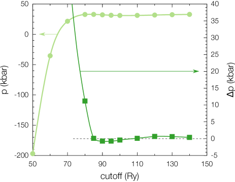
Figure 1: Pressure as a function of the plane-wave energy cutoff for a given structural configuration of liquid water (vertical axis on the left). The second curve represents the difference between the current pressure and that at the previous energy cutoff (vertical axis on the right). The continuous lines are guides to the eye.

The theoretical framework described so far is common to our simulations performed with the two codes: Quantum-EspressoGiannozzi et al. (2009) and CP2K.cp2 (2013) The fundamental difference between the codes rests on the use of different basis sets for the representation of the electron wavefunction. In Quantum-Espresso, the Kohn-Sham orbitals are expanded on plane waves (PW), while core-valence interactions are described by Troullier-Martins norm-conserving pseudopotentials.Troullier and Martins (1991) The PW energy cutoff is set on the basis of convergence tests for the calculated pressure associated to specific liquid water snapshots. As shown in Fig. 1, we verified that by setting the PW energy cutoff at 85 Ry, the pressure is converged within 1 kbar.Miceli, De Gironcoli, and Pasquarello (2015) In the mixed Gaussian-plane-wave scheme (GPW) in CP2K, the core-valence interactions are described by Goedecker-Teter-Hutter pseudopotentials.Goedecker, Teter, and Hutter (1996) The Kohn-Sham orbitals are expanded on a Gaussian basis set,Lippert, Hutter, and Parrinello (1997) while an auxiliary plane waves basis set defined by a cutoff of 800 Ry is used to expand the electron density. We here use the triple-$\zeta$ basis set augmented with polarization functions (TZV2P).VandeVondele and Hutter (2007) This basis set has been validated through BLYP simulations of liquid water.VandeVondele et al. (2005)

We perform Born-Oppenheimer molecular dynamics simulations of liquid water within both the microcanonical (NVE) and the isobaric-isoenthalpic (NpH) statistical ensembles. The Born-Oppenheimer scheme is here preferred to the Car-Parrinello one as it avoids any dependence on fictitious parameters which might affect the MD trajectoryTangney and Scandolo (2002); Grossman et al. (2004) and be basis-set dependent.

The system is modeled using supercells with 64 water molecules subject to periodic boundary conditions. In this work, we neglect nuclear quantum effects. Newton’s equations of motion are integrated with a time step of 0.48 fs to correctly sample the highest frequency of the O-H stretching mode. The energy convergence threshold for selfconsistency at each Born-Oppenheimer MD steps is set to $5\times 10^{-11}$ a.u./atom. In the case of NVE simulations, the conservation of total energies is better than 1 part over 10⁵ over simulation periods of 10 ps, for both the PW and GPW schemes.

The volume of the cell in NVE simulations is fixed at a value corresponding to the experimental water density. On the contrary, in the NpH simulations the cell volume is allowed to fluctuate, but is constrained to preserve the initial cell shape of cubic symmetry. A vanishing external pressure is imposed through the use of a Parrinello-Rahman barostat.Parrinello and Rahman (1980) The statistical analysis is performed on runs at 350 K with duration of about 30 ps each. The latter are preceded by equilibrium runs of 5 to 10 ps.

When using isobaric first-principles molecular dynamics with a constant number of plane waves, the fluctuations of the cell volume imply fluctuations of the effective energy cutoff defining the basis set. Plane-wave basis sets are used by both Quantum-Espresso and CP2K. For this reason, further precautions are needed. In CP2K, a reference cell with a larger volume is used to determine the number of grid points which is then kept fixed regardless of the actual size of the simulation cell.McGrath et al. (2005); Schmidt et al. (2009) In Quantum-Espresso, the MD runs are restarted when the density of the simulation cell reaches excessively low values. The restart at a larger initial volume restores the energy cutoff required for achieving converged results.Miceli, De Gironcoli, and Pasquarello (2015)

For information, we here report the computational performance of the two simulation set-ups as recorded for runs on a Cray XC30 system. Using the same number of processors, we find that the wall-clock time for one MD step is 21.4 s step for Quantum-Espresso and 10.3 s for CP2K. We record linear scaling for both simulation schemes up to 128 cores, with efficiencies of 85% and 90% for Quantum-Espresso and CP2K, respectively.

III Results and discussion

In this section, we compare and discuss the results of structural, dynamical, and electronic properties of liquid water at near ambient conditions obtained using the Quantum-Espresso and CP2K suites of programs. When available, experimental data are reported for comparison.

Isobaric molecular dynamics simulations allow for fluctuations of the system volume. In particular, the volume reaches the equilibrium value at the hydrostatic pressure set externally. As already pointed out previously,Schmidt et al. (2009); Miceli, De Gironcoli, and Pasquarello (2015) first principles methods are able to describe the correct density of liquid water only when the adopted theory explicitly accounts for van der Waals interactions. In particular, using Quantum-Espresso we have shown that the nonlocal rVV10 functional yields an equilibrium water density of 0.99 g/cm³ when the phenomenological parameter $b$ is set to 9.3.Miceli, De Gironcoli, and Pasquarello (2015) By carrying out simulations with the same functional but describing the electronic wave functions and density with the mixed Gaussian-plane-wave scheme implemented in CP2K, we find that liquid water shows a density of 1.01 g/cm³, at the same thermodynamic conditions of 350 K and zero pressure. Using the blocking analysis method,Flyvbjerg and Petersen (1989) we obtain statistical errors of about 0.01 g/cm³ in both cases, indicating that the two codes are in excellent agreement.

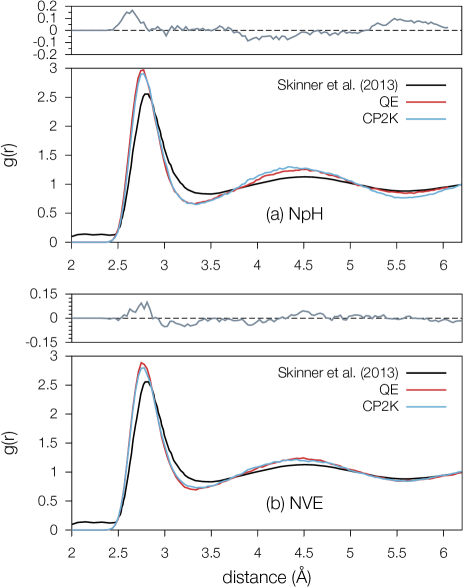
Figure 2: Oxygen-oxygen radial distribution functions resulting from from molecular dynamics trajectories obtained with Quantum-Espresso (QE) and CP2K. For comparison, we superimpose results from the most recent experimental work of Ref. 48. Panels (a) and (b) refer to isobaric-isoenthalpic and microcanonical simulations, respectively. In both cases, the differences $g_{\textrm{{\sc QE}}}(r)-g_{\textrm{\tt CP2K}}(r)$ are reported at the top of the respective panels.

To gain deeper insight into the structural properties of liquid water, we compare the two calculated oxygen-oxygen radial distribution functions, $g_{\textrm{OO}}(r)$. In Fig. 2(a), we show radial distribution functions as obtained through an isobaric-isoenthalpic sampling with the two different codes. The difference $g^{\rm NpH}_{\textrm{{\sc QE}}}(r)-g^{\rm NpH}_{\textrm{\tt CP2K}}(r)$ is reported at the top of panel (a) in the same figure. The experimental curve from Ref. 48 is superimposed. As one can notice, the two calculated $g_{\textrm{OO}}(r)$ are in very good agreement. In both cases the positions of the first peak are found at 2.75 Å. The first peak representing the first coordination shell is barely higher in the Quantum-Espresso simulation. The same kind of agreement is found for the second shell. Compared to experiment, the position of the first peak in the calculated oxygen-oxygen radial distribution function is slightly shifted by 0.05 Å towards shorter distances with respect to the experimental value. The simulated liquid still shows overstructuring with respect to experiment, but the overall description of the system is improved with the respect to the PBE functional, as already pointed out previously.Miceli, De Gironcoli, and Pasquarello (2015)

We also study the structural properties of liquid water obtained in the NVE statistical ensemble. We carry out fixed-volume simulations at the experimental density of 1 g/cm³ using Quantum-Espresso and CP2K at the rVV10-b9.3 level of theory. In Fig. 2(b), we report the calculated oxygen-oxygen radial distribution functions as obtained from these NVE-MD runs. The two calculated $g_{\textrm{OO}}(r)$ basically coincide. Quantum-Espresso gives rise to an imperceptible overstructuring with respect to CP2K at short distances. At longer distances the agreement between the two codes is excellent. More generally, we also observe an excellent agreement between the two codes in reproducing the overall structural properties of the system. Hereafter, all the presented results refer to the microcanonical simulations.

Earlier NVE simulations based on the BLYP functionalKuo et al. (2004) also showed very good agreement between plane-wave and atomic-orbital schemes in describing the structural properties of liquid water. The position and the height of the first peak in the $g_{\rm OO}$ differed by only 0.01 Å and 0.2, to be compared with our differences of 0.00 Å and 0.09, respectively. Together with our NpH results, these comparisons support the general notion that structural properties are well converged in both simulation schemes.

Table 1: Distribution of water molecules with a given number of hydrogen bonds. The percentages correspond to the height of each bar in the histograms shown in Fig. 3. The largest statistical error is found for the fourfold hydrogen-bonded molecules and amounts to 1.1% and 1.7% for Quantum-Espresso and CP2K, respectively. The average number of hydrogen bonds per water molecule is given in the last column and the experimental estimate from Ref. 49 is reported for comparison. The statistical error on the average number of hydrogen bonds is less than 0.01. The statistical errors are estimated by treating nonoverlapping trajectories of the duration of 2.5 ps as indepedent.

	Number of hydrogen bonds
	1	2	3	4	5	average
QE	1%	8%	29%	56%	6%	3.58
CP2K	2%	10%	31%	51%	6%	3.49
Expt.(Ref. 49)	–	–	–	–	–	3.58

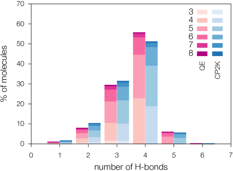
Figure 3: Distributions of water molecules with a given number of hydrogen bonds as obtained with Quantum-Espresso (QE) and CP2K (cf. also Table 1). The finer subdivisions within each bar, here indicated with a gradient of colors, show the associated distribution of the total coordination number. Both the total coordination number and the number of hydrogen bonds are defined using the same cutoff distance of 3.5 Å. For this reason, the former cannot be smaller than the latter.

The anomalous behavior of liquid water has generally been connected to the complex bonding network formed by the water molecules.Mills (1973); Krynicki, Green, and Sawyer (1978) The water network changes with the breaking and the formation of hydrogen bonds as regulated by the considered thermodynamic conditions. A first approximate description of these complex molecular networks can be given by the average number of hydrogen bonds. This quantity is not directly accessible to experiments. However, a value of 3.58 per molecule has been inferred from experimental data for water at ambient conditions.Soper, Bruni, and Ricci (1997) We here define the hydrogen bond using a purely geometrical criterion commonly used in the literature.Luzar and Chandler (1996); Soper, Bruni, and Ricci (1997); Schwegler, Galli, and Gygi (2000); Miceli, De Gironcoli, and Pasquarello (2015) We consider two water molecules to be hydrogen-bonded when their oxygen-oxygen distance is at most 3.5 Å and their hydrogen-bond angle $\angle$OHO is simultaneously larger than 140^∘. Based on this criterion the calculated average number of hydrogen bonds is $(3.58\pm 0.007)$ as obtained with Quantum-Espresso and $(3.49\pm 0.010)$ with CP2K, where the uncertainties are estimated by treating nonoverlapping trajectories of the duration of 2.5 ps as indepedent. The difference between the two simulations exceeds the statistical error estimated in this way, but remains small. Similar values for the average number of hydrogen bonds per molecule have been found through NVE-MD simulations based on other semilocal density functionals.Todorova et al. (2006); Schwegler, Galli, and Gygi (2000) In Table 1, we report the percentage of molecules with a given number of hydrogen bonds. The majority percentage associated to the fourfold hydrogen-bonded molecules is subject to the largest statistical error, which amounts to $\approx$1.1% and $\approx$1.7% for Quantum-Espresso and CP2K, respectively. From the comparison of the results obtained with the two codes, one notices that CP2K gives a slightly lower number of hydrogen bonds when compared to Quantum-Espresso. In fact, water molecules with less than four hydrogen bonds are found to be more likely.

To investigate the local order and the overall structural organization at a higher level detail, we proceed with a finer analysis of the short-range order by calculating the total coordination number of a molecule with a given number of hydrogen bonds. In practice, let us consider the most probable situation in which a molecule shows four hydrogen bonds. Within the cutoff distance of 3.5 Å that defines the first coordination shell, the molecule might show a solvation shell containing more than four water molecules. These results are illustrated in Fig. 3. The heights of the histogram bars correspond to the percentages reported in Table 1, while the gradient of colors within the same bar indicates the percentages of molecules with higher coordination number. We have shown that this further analysis is very sensitive to the adopted theoretical scheme.Miceli, De Gironcoli, and Pasquarello (2015) In particular, we have demonstrated that even though rVV10-b6.3 and rVV10-b9.3 yield very close average numbers of hydrogen bonds (3.55 and 3.59, respectively) the finer distribution illustrating total coordination numbers differs noticeably. In Fig. 3, we show that the two codes produce close results for the hydrogen-bond network also at this finer level of detail.

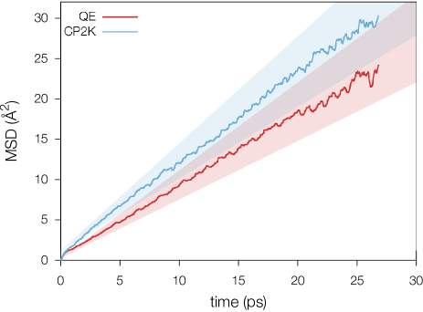
Figure 4: Mean square displacement as a function of time for the NVE-MD runs obtained with Quantum-Espresso (QE) and CP2K. The shaded areas represent an estimation of the statistical errors in evaluating the MSD.

Table 2: Self-diffusion coefficient $D^{\textrm{sim}}$ of liquid water obtained from our NVE-MD runs obtained with Quantum-Espresso (QE) and CP2K. The calculated values are compared to reference values $D^{\textrm{ref}}$, which represent the experimental diffusion coefficient modified to account for the finite-size effect pertaining to the cell size used in the simulations. For reference, we also report the actual experimental data extracted from Ref. 54.

	$T$ (K)	$D^{\textrm{sim}}$ (cm2/s)	$D^{\textrm{ref}}$ (cm2/s)
QE	350	$(1.50\pm 0.30)\cdot 10^{-5}$	$4.3\cdot 10^{-5}$
CP2K	350	$(1.80\pm 0.36)\cdot 10^{-5}$	$4.3\cdot 10^{-5}$
			$D^{\textrm{expt.}}$ (cm2/s)
Expt.(extrapolated)	350		$6.2\cdot 10^{-5}$
Expt.	300		$2.4\cdot 10^{-5}$

We calculate the self-diffusion coefficient of liquid water using Einstein’s relation. The mean square displacement (MSD) as a function of time results from averaging over all water molecules. We average over the NVE-MD trajectories choosing initial times separated by 2 ps. In Fig. 4, we report the MSDs as a function of time and the respective diffusion coefficients with their relative statistical errors are summarized in Table 2. We estimate the statistical errors on the diffusion coefficients by performing a large set of independent molecular dynamics simulations based on an empirical force field. For this, we use simulations with the same set-up (duration, supercell size, thermodynamic conditions) as for the ab initio MD. The resulting percent error on the self-diffusion coefficient is then assumed to apply to the ab initio MD. Within the statistical errors determined in this way the two codes give consistent diffusion coefficients. For comparison, in an earlier comparison of the same kind, Kuo et al. found diffusion coefficients with relative differences ranging between 25% and 50% of the plane-wave result.Kuo et al. (2004) At variance, the comparison with the complete-basis-set simulations achieved with a discrete variable representation Lee and Tuckerman (2006, 2007) cannot directly be compared with our results. Indeed, the latter simulations have been carried out with the Car-Parrinello method, which leads to biased diffusion coefficients.Tangney and Scandolo (2002); Grossman et al. (2004); Kuo et al. (2004)

The comparison of the calculated values with experiments requires some care. In fact, it is well known that dynamical properties suffer from finite-size effects more than structural properties. Generally, this leads to an underestimation of the self-diffusion coefficient. To account for the finite-size effect, we compare the calculated diffusion coefficients $D^{\textrm{sim}}$ with reference values $D^{\textrm{ref}}$, derived from experimental data. Here, $D^{\textrm{ref}}$ represents the experimental self-diffusion coefficient at the temperature of 350 K, modified to account for the cell size used in the simulation.Miceli, De Gironcoli, and Pasquarello (2015) We notice that, although the rVV10-b9.3 functional improves the description of the dynamical properties of liquid water, the experimental value is still underestimated by about a factor 2.5 at this level of theory.

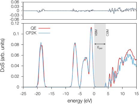
Figure 5: Electronic density of states averaged over 20 configurations of liquid water, separated by 50 fs, taken from the tail of the NVE-MD trajectories. The electronic structures calculated with the two codes are aligned through the valence band edge and their difference is plotted in the upper part of the panel. The shaded region represents the band gap.

Table 3: Energy-level separations obtained by averaging over the Quantum-Espresso (QE) and CP2K MD trajectories. $\varepsilon_{\rm c}$, $\varepsilon_{\rm v}$, and $\varepsilon_{{\rm O}2s}$ refer to the conduction band edge, the valence band edge and the average level of O 2$s$, respectively. The statistical errors are given in parentheses. Energies are given in eV.

	$\varepsilon_{\rm v}-\varepsilon_{{\rm O}2s}$	$\varepsilon_{\rm c}-\varepsilon_{{\rm O}2s}$	$\varepsilon_{\rm c}-\varepsilon_{\rm v}$
QE	18.61 (0.016)	22.71 (0.004)	4.10 (0.016)
CP2K	18.72 (0.016)	22.92 (0.005)	4.20 (0.016)

Next, we focus on the electronic structure of liquid water. Describing its electronic properties does not only have a fundamental interest, but is also critical for applications involving the water splitting process. In Fig. 5, we compare the electronic density of states of liquid water as obtained with Quantum-Espresso and CP2K. These have been obtained via a statistical average over 20 different water configurations regularly spaced by 50 fs, which have been extracted from the NVE-MD trajectories at 350 K. The two electronic structures are superimposed and aligned through the valence band edge. The results from the two codes are in excellent agreement. As one can see from the difference of the two curves in the upper part of Fig. 5, imperceptible differences are present for occupied states. The two curves slightly depart from each other for the unoccupied states at higher energies. The latter behavior should be ascribed to the use of different basis sets for the expansion of the electronic wave functions in the two codes.

From a theoretical point of view, the definition of band gap for a disordered insulator might lead to ambiguities and be subject to finite size effects.Ambrosio, Miceli, and Pasquarello (2015) Nevertheless, these issues do not apply here because we are interested in comparing two codes for simulations with identical supercells. The band gap is thus determined as the energy difference between the lowest unoccupied (LUMO) and the highest occupied (HOMO) molecular orbitals over the molecular dynamics trajectory. In Table 3, we report the calculated values for the band gap ($\varepsilon_{\rm c}-\varepsilon_{\rm v}$) and for the conduction and valence band-edge positions with respect to the average O 2$s$ level ($\varepsilon_{\rm v}-\varepsilon_{{\rm O}2s}$ and $\varepsilon_{\rm c}-\varepsilon_{{\rm O}2s}$, respectively). The determined band gaps are 4.10 and 4.20 eV as obtained with Quantum-Espresso and CP2K, respectively. The energy separations $\varepsilon_{\rm v}-\varepsilon_{{\rm O}2s}$ similarly agree within 0.1 eV. For $\varepsilon_{\rm c}-\varepsilon_{{\rm O}2s}$, the difference is only slightly larger (0.2 eV). Overall, This close accord for the electronic levels further supports the agreement between the two codes.

IV Conclusions

In this work, we compare results obtained through NpH and NVE molecular dynamics simulations performed using plane-wave and atomic-orbital basis sets, as implemented in Quantum-Espresso and CP2K, respectively. In both frameworks, we used the same nonlocal density functional approximation accounting for van der Waals interactions. Noticeably, the schemes based on plane waves and atomic orbitals yield results for structural, dynamical, and electronic properties in overall very good agreement with each other. Hence, the quality of this agreement allows one to envisage equivalently the use of either implementation in the study of liquid water or aqueous solutions.